Electromagnetic vacuum stresses and energy fluxes induced
by a cosmic string in de Sitter spacetime

Abstract

For the electromagnetic field in $(D+1)$-dimensional locally de Sitter (dS) spacetime, we analyze the effects of a generalized cosmic string type defect on the vacuum expectation value of the energy-momentum tensor. For the Bunch-Davies vacuum state, the topological contributions are explicitly extracted in both the diagonal and off-diagonal components. The latter describes the presence of radially directed energy flux in the vacuum state. It vanishes for $D=3$ because of the conformal invariance of the electromagnetic field and is directed towards the cosmic string for $D\geq 4$. The topological contributions in the vacuum stresses are anisotropic and, unlike to the geometry of a cosmic string in the Minkowski spacetime, for $D>3$ the stresses along the directions parallel to the string core differ from the energy density. Depending on the planar angle deficit and the distance from the cosmic string, the corresponding expectation values can be either positive or negative. Near the cosmic string the effect of the gravitational field on the diagonal components of the topological part is week and the leading terms in the respective expansions coincide with the expectation values for a cosmic string in background of Minkowski spacetime. The spacetime curvature essentially modifies the behavior of the topological terms at proper distances from the cosmic string larger than the dS curvature radius. In that region, the topological contributions in the diagonal components of the energy-momentum tensor decay in inverse proportion to the fourth power of the proper distance and the energy flux density behaves as inverse-fifth power for all values of the spatial dimension $D$. The exception is the energy density in the special case $D=4$. For a cosmic string in the Minkowski bulk the energy flux is absent and the diagonal components are proportional to the $(D+1)$th power of the inverse distance.

Keywords: Cosmic string, de Sitter spacetime, electromagnetic vacuum

1 Introduction

The canonical quantization of fields is based on the expansion of the field operator in terms of a complete set of mode functions being the solutions of the classical field equation. That expansion defines the annihilation and creation operators and then the space of the Fock states is constructed. The vacuum is defined as a state of a quantum field that is nullified by the action of the annihilation operator. The mode functions employed in the quantization procedure reflect both the local and global properties of background spacetime and the same holds for the vacuum state. In particular, among the interesting directions in the investigations of the quantum vacuum is the dependence of its properties on the spatial topology. Here we study the polarization of the electromagnetic vacuum on background of $(D+1)$-dimensional de Sitter (dS) spacetime in the presence of a topological defect that is a generalization of a straight cosmic string in (3+1)-dimensional spacetime. The cosmic strings are formed in the early universe as a result of symmetry breaking phase transitions (for reviews see [1, 2, 3, 4]). The interior energy density of those defects is determined by the energy scale at which the phase transition takes place and the observation of cosmic strings at recent epoch of the universe expansion may provide an important window to high-energy physics. The gravitational field around of those kinds of topological defects is a source of a number of physical effects including the gravitational lensing, the generation of gravitational waves and gamma ray bursts. The cosmic strings also give rise to non-Gaussian distorsions in the fluctuations of the cosmic microwave background [5].

Our consideration of dS spacetime as a background geometry is motivated by several reasons. First of all, its high degree of symmetry allows to obtain closed analytic expressions for the cosmic string induced local characteristics of the vacuum state. This will shed light on combined effects of local geometry and topology in more complicated backgrounds. Another reason is related to the profound role of dS spacetime in cosmology. The most inflationary models employ the dS exponential expansion in the early universe to provide natural solutions to a number of problems in the Standard Big-Bang cosmology (see [6, 7, 8]). From the other side, the observational data on the temperature anisotropies of cosmic microwave background, high redshift supernovae and galaxy clusters [9]-[15] indicate that the recent expansion of the universe is dominated by a source of the cosmological constant type. The relative contribution of the latter to the total energy density will increase during the expansion and the corresponding geometry asymptotes dS spacetime in the future.

The quantum field-theoretical effects in fixed dS background were investigated in a large number of papers. Different coordinate systems have been considered, including global, planar, static and hyperbolic coordinates. In particular, motivated by an important role of vacuum fluctuations during the inflationary phase in the formation of large scale structures in the post inflationary era, the dynamics of vacuum fluctuations of scalar fields have attracted great deal of attention. The properties of those fluctuations are encoded in the observed spectrum of temperature anisotropies for cosmic microwave background radiation and this opens a possibility to test the effects of gravity on quantum matter. A similar amplification of the electromagnetic field quantum fluctuations by the dS expansion can serve as a mechanism for the generation of extragalactic magnetic fields. However, for this mechanism to work, it is required to break the conformal invariance of the electromagnetic field in (3+1)-dimensional spacetime. That can be done by an additional coupling of the electromagnetic field with other degrees of freedom, for example, by adding a factor in the Maxwell kinetic term that depends on other fields. Another possibility for breaking the conformal symmetry is to consider models with extra spatial dimensions (for the generation of large scale magnetic fields in those types of models see, for example, [16, 17, 18]). This is one of the reasons for our discussion of background spacetime with general number of dimensions. Another reason is that the background geometry we consider can also be generated by fundamental strings in superstring theories. A mechanism for the formation of those types of objects within the framework of brane inflation models has been discussed in [5, 19, 20, 21]. In models with fundamental strings as cosmic strings, depending upon the number of compact dimensions, the spatial dimension of the effective theory may vary from 3 to 9.

The polarization of vacuum by a cosmic string has been widely considered in the literature for both neutral and charged quantum fields. That was mainly done for an idealized model where the influence of cosmic string on the spacetime geometry outside the core is reduced to the generation of planar angle deficit determined by the energy density inside the core. Exact analytic results for the local characteristics of the vacuum are obtained for highly symmetric background geometries, including Minkowski, dS and anti-de Sitter (AdS) spacetimes. Cosmic string type topological defects in dS and AdS spacetimes were considered in [22]-[27]. The influence of the cosmological expansion on the properties of scalar vacuum around a straight cosmic string in flat Friedmann-Robertson-Walker type models has been discussed in [28] for special values of the planar angle deficit $2\pi-\phi_{0}$ corresponding to integer values of the parameter $q=2\pi/\phi_{0}$. For those values the Green function in a conical space is expressed as an image sum over the Green functions in the absence of cosmic string. The vacuum polarization around a straight cosmic string in dS spacetime for general values of the planar angle deficit in the cases of massive scalar and fermionic fields has been investigated in [29, 30]. The correlators for the electromagnetic field and the vacuum expectation values of the electric and magnetic fields squared were discussed in [31, 32]. Additional topological effects on the properties of the scalar and fermionic vacua induced by compactification of a cosmic string along its axis in locally dS bulk were studied in [33, 34, 35]. The polarization of the scalar and fermionic vacua around a cosmic string in background of AdS spacetime has been investigated in [36, 37]. The combined effects of a cosmic string, compact dimensions and branes on the local characteristics of the vacuum in locally AdS spacetime were discussed in [38]-[43]. The finite temperature effects on the expectation values of the charge and current densities for a charged scalar field in the presence of a cosmic string and compact dimension on locally AdS bulk were considered recently in [44].

The organization of the present paper is as follows. The problem setup and the mode functions for the electromagnetic field are presented in the following section. Section 3 considers the vacuum expectation values (VEVs) for the diagonal components of the energy-momentum tensor. The contributions induced by the cosmic string are separated explicitly and their asymptotics are investigated. Special cases are discussed and the results of numerical analysis are presented. In addition to the diagonal components, the vacuum energy-momentum tensor has a nonzero off-diagonal component that describes energy flux along the radial direction. This is a cosmic string induced effect and is studied in Section 4. The main results of the paper are summarized in Section 5.

2 Setup and electromagnetic mode functions

As a background geometry we consider $(D+1)$-dimensional spacetime having the line element

$$ds^{2}=dt^{2}-e^{2t/\alpha}[dr^{2}+r^{2}d\phi^{2}+\left(d\mathbf{z}\right)^{2}],$$ (2.1)

where $\mathbf{z=}\left(z^{3},...,z^{D}\right)$ with $-\infty<z^{i}<+\infty$, $-\infty<t<+\infty$, $0\leqslant r<\infty$, and $0\leqslant\phi\leqslant\phi_{0}$. In the special case $\phi_{0}=2\pi$ this line element describes $(D+1)$-dimensional dS spacetime sourced by the cosmological constant $\Lambda=D(D-1)/(2\alpha^{2})$ and foliated by flat spaces with cylindrical coordinates $(r,\phi,\mathbf{z})$. For $\phi_{0}<2\pi$ and at the points $r>0$ the local geometrical characteristics coincide with those for dS spacetime. In particular, for the Ricci scalar one has $R=D(D+1)/\alpha^{2}$. The geometry described by (2.1) is a generalization of an idealized cosmic string, being a linear topological defect in $D=3$, for spatial dimensions $D>3$. The defect core, given by $r=0$, presents a $(D-2)$-dimensional spatial hypersurface. Introducing the new time coordinate $\tau$ in accordance with $\tau=-\alpha e^{-t/\alpha}$, $-\infty<\tau<0$, the line element is written in the form conformally flat for $r>0$:

$$ds^{2}=\frac{\alpha^{2}}{\tau^{2}}[d\tau^{2}-dr^{2}-r^{2}d\phi^{2}-\left(d\mathbf{z}\right)^{2}].$$ (2.2)

Similar to the case of the Minkowski bulk, for the model with $D=3$ the deficit angle $2\pi-\phi_{0}$ in dS spacetime is induced by the vortex solution of the Einstein-Abelian-Higgs equations in the presence of a cosmological constant [22].

In quantum field theory the notion of the vacuum state, denoted as $|0\rangle$, has a global nature and its properties are sensitive to both local and global characteristics of the background spacetime. In the geometry under consideration, the nontrivial spatial topology induced by the planar angle deficit gives rise to additional vacuum polarization for quantum fields. Here we are interested in the topological effects on the VEV of the energy-momentum tensor $T_{i}^{l}$ for the electromagnetic field with the vector potential $A_{i}(x)$. Our approach for evaluation of the expectation value $\langle 0|T_{i}^{l}|0\rangle\equiv\langle T_{i}^{l}\rangle$ will be based on the direct summation over the complete set of electromagnetic modes for the background geometry (2.2). We will denote by $\{A_{(\beta)i}(x),A_{(\beta)i}^{\ast}(x)\}$ the corresponding set for the vector potential, where $\beta$ is the collective notation for the quantum numbers specifying the solutions of Maxwell’s equations in $(D+1)$-dimensional spacetime. With $F_{(\beta)lm}=\partial_{l}A_{(\beta)m}-\partial_{m}A_{(\beta)l}$ being the electromagnetic field tensor for the modes, the mode-sum for the vacuum energy-momentum tensor is expressed as

$$\langle T_{i}^{l}\rangle=\frac{1}{4\pi}\underset{\beta}{\sum}\left[\frac{1}{4}\delta_{i}^{l}F_{(\beta)}^{mn}F_{(\beta)mn}^{\ast}-F_{(\beta)i}^{\cdot m}F_{(\beta)\cdot m}^{l\ast}\right],$$ (2.3)

where $F_{(\beta)}^{il}=g^{im}g^{ln}F_{(\beta)mn}$. In what follows it is convenient to work in the coordinates $(\tau,r,\phi,\mathbf{z})$ with the metric tensor $g_{il}=\left(\alpha/\tau\right)^{2}\mathrm{diag}(1,-1,-r^{2},-1,\ldots,-1)$. We will fix the vector potential by the gauge conditions $A_{0}=0$ and $\sum_{i=1}^{D}\partial_{i}(\sqrt{|g|}A^{i})=0$ with $\sqrt{|g|}=\left(\alpha/\eta\right)^{D+1}r$ and $\eta=|\tau|$.

The electromagnetic cylindrical modes have been discussed in [45] for $(D+1)$-dimensional dS spacetime and were generalized for the presence of a cosmic string in [31]. One has $D-1$ polarization states and we will distinguish them by the index $\sigma=1,\ldots,D-1$.  In addition to this quantum number, the electromagnetic modes are specified by the wave vector $\mathbf{k}=(k_{3},\ldots,k_{D})$ in the subspace covered by the coordinates $\mathbf{z}$, by the radial quantum number $\gamma$, $0\leq\gamma<\infty$, and by the azimuthal quantum number $m$, $m=0,\pm 1,\pm 2,\ldots$. Consequently, the set $\beta$ is specified as $(\beta)=(\gamma,m,\mathbf{k},\sigma)$. Introducing the notation $q=2\pi/\phi_{0}$, the vector potentials for separate polarizations are expressed as [31]

$$A_{(\beta)l}(x) = \eta^{\frac{D}{2}-1}Z_{\frac{D}{2}-1}(\omega\eta)\left\{\begin{array}[]{c}\left(0,iqm/r,-r\partial_{r},0,\ldots,0\right)\\ \left(0,\omega\epsilon_{\sigma n}+i\omega^{-1}\mathbf{k}\cdot{\boldsymbol{\epsilon}}_{\sigma}\partial_{n}\right)\end{array}\right.$$ (2.9)

$$\times J_{q|m|}(\gamma r)e^{iqm\phi+i\mathbf{k}\cdot\mathbf{z}},\;\begin{array}[]{l}\sigma=1\\ \sigma=2,\ldots,D-1\end{array},$$

where $\omega=\sqrt{\gamma^{2}+|\mathbf{k}|^{2}}$, $n=1,\ldots,D$, $J_{\nu}(y)$ is the Bessel function, $\mathbf{k}\cdot\mathbf{z}=\sum_{i=3}^{D}k_{i}z^{i}$, and $\mathbf{k}\cdot{\boldsymbol{\epsilon}}_{\sigma}=\sum_{i=3}^{D}k_{i}\epsilon_{\sigma i}$, with $\epsilon_{\sigma 1}=\epsilon_{\sigma 2}=0$. In (2.9), the function $Z_{\nu}(y)$ is the linear combination of the Hankel functions $H_{\nu}^{(1)}(y)$ and $H_{\nu}^{(2)}(y)$, $Z_{\nu}(y)=\sum_{i=1,2}c_{\beta}^{(i)}H_{\nu}^{(i)}(y)$. The polarization vectors ${\boldsymbol{\epsilon}}_{\sigma}$ obey the orthonormalization condition

$$\sum_{l,n=3}^{D}\left(\delta_{nl}-\frac{k_{l}k_{n}}{\omega^{2}}\right)\epsilon_{\sigma l}\epsilon_{\sigma^{\prime}n}=\frac{\gamma^{2}}{\omega^{2}}\delta_{\sigma\sigma^{\prime}}.$$ (2.10)

The orthonormalization condition for the mode functions is written as

$$\int d^{D}x\sqrt{|g|}[A_{(\beta^{\prime})l}^{\ast}\nabla^{0}A_{(\beta)}^{l}-(\nabla^{0}A_{(\beta^{\prime})l}^{\ast})A_{(\beta)}^{l}]=4i\pi\delta(\gamma-\gamma^{\prime})\delta(\mathbf{k}-\mathbf{k}^{\prime})\delta_{mm^{\prime}}\delta_{\sigma\sigma^{\prime}},$$ (2.11)

where $\nabla^{i}=g^{ik}\nabla_{k}$ and $\nabla_{k}$ is the covariant derivative operator. This condition determines the one of the coefficients $c_{\beta}^{(i)}$ in the linear combination of the Hankel functions in the definition of the function $Z_{\nu}(y)$. Similar to that for pure dS bulk, the second coefficient is fixed by the choice of the vacuum state. Here we will assume that the electromagnetic field is prepared in the state that is the analog of the Bunch-Davies vacuum for a scalar field in dS spacetime. For that state $c_{\beta}^{(2)}=0$ and in the expressions (2.9) for the mode functions

$$Z_{\frac{D}{2}-1}(\omega\eta)=c_{\beta}^{(1)}H_{\frac{D}{2}-1}^{(1)}(\omega\eta).$$ (2.12)

With this choice, the normalization coefficient is found from (2.11):

$$|c_{\beta}^{(1)}|^{2}=\frac{q}{4(2\pi\alpha)^{D-3}\gamma}.$$ (2.13)

Note that this coefficient is the same for all the polarizations.

For $D=3$ one has $\eta^{D/2-1}H_{D/2-1}^{(1)}(\omega\eta)=-ie^{-i\omega\tau}\sqrt{2/\pi\omega}$ and the mode functions (2.9) coincide with those for a cosmic string in the Minkowski bulk. Of course, this is a consequence of the conformal invariance of the electromagnetic field in 4-dimensional spacetime. For $D>3$ and in the limit $\alpha\rightarrow\infty$ for a fixed value of the synchronous time $t$, from (2.9) the mode functions are obtained for a cosmic string in $(D+1)$-dimensional Minkowski bulk.

3 Diagonal components of the energy-momentum tensor

Having the complete set of the electromagnetic modes we can evaluate the VEV of the energy-momentum tensor by making use of the formula (2.3). The expression in the right-hand side of (2.3) is divergent and a regularization is required. For example, the point splitting procedure can be employed with the combination of the two-point functions from [31] (for vector field correlators in dS spacetime see [46]-[53] and references therein). Another possibility is to introduce a cutoff function, for example, in the form $e^{-b\omega^{2}}$ with the cutoff parameter $b>0$. The important point to be mentioned is the following. For $r>0$ the local geometry in the presence of the cosmic string is the same as that for the pure dS spacetime and, hence, for those points the divergences in the VEV of the energy-momentum tensor are the same as well. From here it follows that if one extracts explicitly the part in the regularized VEV corresponding to the pure dS geometry, then the renormalization is required for that part only. The remaining topological contribution is finite in the limit when the regularization is removed. Below we will extract the pure dS part and the specific regularization scheme is not essential in that procedure. In the evaluation of the diagonal components we will regularize the expectation values by introducing the cutoff function $e^{-b\omega^{2}}$.

3.1 General expressions

Substituting the modes (2.9) in (2.3) with the cutoff function $e^{-b\omega^{2}}$ and by using the relation [31]

$$\sum_{\sigma=2}^{D-1}\epsilon_{\sigma n}\epsilon_{\sigma l}=\frac{\gamma^{2}\delta_{nl}+k_{n}k_{l}}{\omega^{2}},$$ (3.1)

with $l,n=3,...,D$, for summation over the polarization states, the regularized diagonal components of the vacuum energy-momentum tensor are expressed as (no summation over $i$)

$$\langle T_{i}^{i}\rangle_{\mathrm{reg}} = \frac{2^{2-D}q\eta^{D+2}}{\pi^{D/2+1}\Gamma(D/2-1)\alpha^{D+1}}\sideset{}{{}^{\prime}}{\sum}_{m=0}^{\infty}\int_{0}^{\infty}dk\,k^{D-3}\int_{0}^{\infty}d\gamma\gamma e^{-b\omega^{2}}$$ (3.2)

$$\times\sum_{l=1,2}t_{l}^{(i)}[k,\gamma,J_{qm}(\gamma r)]K_{\frac{D}{2}-l}(\omega\eta e^{-i\pi/2})K_{\frac{D}{2}-l}(\omega\eta e^{i\pi/2}),$$

where $k=|\mathbf{k}|$, $K_{\nu}(x)$ is the Macdonald function. The prime on the sign of summation means that the term $m=0$ is taken with coefficient 1/2. The Macdonald function is introduced instead of the Hankel function in the expression for the electromagnetic modes. In (3.2), the function containing the radial dependence is defined as

$$t_{l}^{(i)}\left[k,\gamma,f\left(y\right)\right]=(a_{l}^{(i)}k^{2}+b_{l}^{(i)}\gamma^{2})\left[f^{\prime 2}(y)+\delta_{i}\frac{q^{2}m^{2}}{y^{2}}f^{2}(y)\right]+\left[\left(D-3\right)c_{l}^{(i)}k^{2}+d_{l}^{(i)}\gamma^{2}\right]f^{2}(y),$$ (3.3)

where

$$\delta_{i}=\left\{\begin{array}[]{ll}1,&i=0,3,\ldots,D\\ -1,&i=1,2\end{array}\right..$$ (3.4)

For the coefficients in the definition of the function $t_{l}^{(i)}\left[k,\gamma,f\left(y\right)\right]$ one has

$$a_{l}^{(0)} = \left(2,2\right),\;b_{l}^{(0)}=\left(D-2,1\right),\;c_{l}^{(0)}=\left(1,1\right),\;d_{l}^{(0)}=\left(1,D-2\right),$$

$$a_{l}^{(1)} = \left(0,0\right),\;b_{l}^{(1)}=\left(2-D,-1\right),\ c_{l}^{(1)}=\left(1,-1\right),\;d_{l}^{(1)}=\left(-1,2-D\right),$$

$$a_{l}^{(2)} = \left(0,0\right),\;b_{l}^{(2)}=\left(D-2,1\right),\;c_{l}^{(2)}=\left(1,-1\right),\;d_{l}^{(2)}=\left(-1,2-D\right),$$ (3.5)

and

$$a_{l}^{(p)} = \left(2\frac{D-4}{D-2},-2\right),\;b_{l}^{(p)}=\left(D-4,-1\right),$$

$$c_{l}^{(p)} = \left(\frac{D-6}{D-2},\frac{4-D}{D-2}\right),\;d_{l}^{(p)}=\left(1,4-D\right),$$ (3.6)

for $p=3,\ldots,D$. Here, the first and second terms correspond to $l=1$ and $l=2$, respectively.

For the further transformation of (3.2) we use the integral representation [54]

$$K_{\nu}(\omega\eta e^{-i\pi/2})K_{\nu}(\omega\eta e^{i\pi/2})=\frac{1}{2}\int_{0}^{\infty}\frac{dx}{x}\exp\left(-\omega^{2}\frac{x}{4}+\eta^{2}\frac{2}{x}\right)K_{\nu}\left(2\eta^{2}/x\right),$$ (3.7)

for the product of the Macdonald functions. Substituting in (3.2), after integration over $k$ we get (no summation over $i$)

$$\langle T_{i}^{i}\rangle_{\mathrm{reg}} = \frac{2^{-D}q\eta^{D+2}}{\pi^{D/2+1}\alpha^{D+1}}\sideset{}{{}^{\prime}}{\sum}_{m=0}^{\infty}\int_{0}^{\infty}\frac{dx}{x}u^{D/2}e^{2\eta^{2}/x}\int_{0}^{\infty}d\gamma\gamma e^{-\gamma^{2}/u}$$ (3.8)

$$\times\sum_{l=1,2}t_{l}^{(i)}(\gamma^{2}/u,J_{qm}(\gamma r))K_{\frac{D}{2}-l}(2\eta^{2}/x),$$

where $u=4/(x+4b)$ and

$$t_{l}^{(i)}(v,f\left(y\right)) = \left[\left(\frac{D}{2}-1\right)a_{l}^{(i)}+b_{l}^{(i)}v\right]\left[f^{\prime 2}(y)+\delta_{i}\frac{q^{2}m^{2}}{y^{2}}f^{2}(y)\right]$$ (3.9)

$$+\left[\left(D-3\right)\left(\frac{D}{2}-1\right)c_{l}^{(i)}+d_{l}^{(i)}v\right]f^{2}(y).$$

The integrals over $\gamma$ are evaluated on the base of the formula [55]

$$\int_{0}^{\infty}d\gamma\ \gamma e^{-\gamma^{2}/u}J_{qm}^{2}(\gamma r)=\frac{u}{2}e^{-r^{2}u/2}I_{qm}(r^{2}u/2),$$ (3.10)

with $I_{\nu}(x)$ being the modified Bessel function, and by using the formulas presented in [31]. This gives (no summation over $i$)

$$\langle T_{i}^{i}\rangle_{\mathrm{reg}} = \frac{(\eta/r)^{D+2}q}{2^{D/2}\pi^{D/2+1}\alpha^{D+1}}\sideset{}{{}^{\prime}}{\sum}_{m=0}^{\infty}\int_{0}^{\infty}\frac{dx}{x}w^{D/2+1}e^{2\eta^{2}/x}$$ (3.11)

$$\times\sum_{l=1,2}K_{\frac{D}{2}-l}(2\eta^{2}/x)\hat{W}_{l}^{(i)}\left(e^{-w}I_{qm}(w)\right),$$

where $w=2r^{2}/(x+4b)$ and the operators $\hat{W}_{l}^{(i)}$ are defined by the expression

$$\hat{W}_{l}^{(i)}=b_{l}^{(i)}w\partial_{w}^{2}+\left[(D/2-1)a_{l}^{(i)}+b_{l}^{(i)}(1+w)+d_{l}^{(i)}w\right]\partial_{w}+e_{l}^{(i)},$$ (3.12)

for the components with $i=0,3,...,D,$ and

by

$$\hat{W}_{l}^{(i)}=(d_{l}^{(i)}-b_{l}^{(i)})w\partial_{w}+e_{l}^{(i)},$$ (3.13)

for $i=1,2$. Here the notations

$$e_{l}^{(0)}=\frac{D-1}{2}\left(D,D\right),\;e_{l}^{(i)}=\frac{D-1}{2}\left(D-4,2-D\right),$$ (3.14)

are introduced with $i=1,2,\ldots,D$.

Next, in order to separate the topological contribution, we use the formula [56]

$$q\sideset{}{{}^{\prime}}{\sum}_{m=0}^{\infty}e^{-w}I_{qm}\left(w\right)=\sideset{}{{}^{\prime}}{\sum}_{j=0}^{[q/2]}e^{-2ws_{j}^{2}}-\frac{q}{\pi}\sin(q\pi)\int_{0}^{\infty}dz\frac{e^{-2w\cosh^{2}z}}{\cosh(2qz)-\cos(q\pi)},$$ (3.15)

where $s_{j}=\sin(j\pi/q)$ and $[q/2]$ is the integer part of $q/2$. The prime on the summation sign in the right-hand side means that the terms $j=0$ and $j=q/2$ (for even values of $q$) should be taken with additional coefficient $1/2$. In the case $q=1$ the $j=0$ term remains only. This shows that the part in the VEV corresponding to the $j=0$ term in (3.15) corresponds to the regularized VEV of the energy-momentum tensor in dS spacetime in the absence of the cosmic string. It is presented as (no summation over $i$)

$$\langle T_{i}^{i}\rangle_{\mathrm{reg}}^{\mathrm{(dS)}}=\frac{\alpha^{-D-1}}{\left(2\pi\right)^{D/2+1}}\int_{0}^{\infty}dy\frac{y^{D/2}e^{y}}{(1+2by/\eta^{2})^{D/2+1}}\sum_{l=1,2}K_{\frac{D}{2}-l}(y)e_{l}^{(i)}.$$ (3.16)

The renormalized VEV of the energy-momentum tensor in dS spacetime, $\langle T_{i}^{l}\rangle_{\mathrm{ren}}^{\mathrm{(dS)}}$, has been widely investigated in the literature and our main concern here will be the cosmic string induced contribution. From the maximal symmetry of the dS spacetime and of the Bunch-Davies vacuum state the structure $\langle T_{i}^{l}\rangle_{\mathrm{ren}}^{\mathrm{(dS)}}=\mathrm{const}\cdot\delta_{i}^{l}$ is expected for the geometry in the absence of the cosmic string.

For the topological part induced by the cosmic string one has (no summation over $i$)

$$\langle T_{i}^{i}\rangle_{\mathrm{t}}=\underset{b\rightarrow 0}{\lim}\left[\langle T_{i}^{i}\rangle_{\mathrm{reg}}-\langle T_{i}^{i}\rangle_{\mathrm{reg}}^{\mathrm{(dS)}}\right].$$ (3.17)

For $r>0$ the limit in the right-hand side is finite. From (3.11), by using (3.15), we find the following representation (no summation over $i$)

$$\langle T_{i}^{i}\rangle_{\mathrm{t}}=\frac{2\alpha^{-D-1}}{(2\pi)^{D/2+1}}\left[\sideset{}{{}^{\prime}}{\sum}_{j=1}^{[q/2]}t^{(i)}\left(r/\eta,s_{j}\right)-\frac{q}{\pi}\sin(q\pi)\int_{0}^{\infty}dz\frac{t^{(i)}\left(r/\eta,\cosh z\right)}{\cosh(2qz)-\cos(q\pi)}\right].$$ (3.18)

In (3.18) we have used the notation

$$t^{(i)}(x,y)=\int_{0}^{\infty}duu^{\frac{D}{2}}e^{u-2ux^{2}y^{2}}\sum_{l=1,2}K_{\frac{D}{2}-l}(u)f_{l}^{(i)}(x,y,u),$$ (3.19)

with the functions

$$f_{l}^{(i)}(x,y,u)=\left[4b_{l}^{(i)}ux^{2}y^{2}-2(b_{l}^{(i)}+d_{l}^{(i)})ux^{2}-((D-2)a_{l}^{(i)}+2b_{l}^{(i)})\right]y^{2}+e_{l}^{(i)},$$ (3.20)

for $i=0,3,...,D$, and

$$f_{l}^{(i)}(x,y,u)=2(b_{l}^{(i)}-d_{l}^{(i)})ux^{2}y^{2}+e_{l}^{(i)},$$ (3.21)

for $i=1,2$. The topological part of the VEV depends on $\eta$ and $r$ in the form of the ratio $r/\eta$. This property is a consequence of the maximal symmetry of dS spacetime. By considering that $\alpha r/\eta$ is the proper distance from the string, we see that $r/\eta$ is the proper distance, measured in units of the dS curvature scale $\alpha$.

Note that the function (3.19) can also be written in the form

$$t^{(i)}(x,y) = 2\int_{0}^{\infty}du\,u^{\frac{D}{2}}e^{u-2ux^{2}y^{2}}\sum_{l=1,2}K_{\frac{D}{2}-l}(u)$$ (3.22)

$$\times\left[2a_{li}^{(4)}ux^{2}y^{4}+a_{li}^{(3)}ux^{2}y^{2}+a_{li}^{(2)}y^{2}+\frac{D-1}{4}a_{li}^{(1)}\right],$$

with $i=0,1,2,3$. The coefficients are given by the expressions

$$a_{li}^{(1)} = \left(\begin{array}[]{cccc}D&D-4&D-4&D-4\\ D&2-D&2-D&2-D\end{array}\right),$$ (3.25)

$$a_{li}^{(2)} = \left(\begin{array}[]{cccc}2\left(2-D\right)&0&0&2(4-D)\\ 1-D&0&0&D-1\end{array}\right),$$ (3.28)

and

$$a_{li}^{(3)} = \left(\begin{array}[]{cccc}1-D&3-D&D-1&3-D\\ 1-D&D-3&D-1&D-3\end{array}\right),$$ (3.31)

$$a_{li}^{(4)} = \left(\begin{array}[]{cccc}D-2&0&0&D-4\\ 1&0&0&-1\end{array}\right).$$ (3.34)

For odd values of $D$ the integral in (3.22) is expressed in terms of elementary functions. By analogy with an ideal fluid, the diagonal components $\langle T_{i}^{i}\rangle_{\mathrm{t}}$ of the energy-momentum tensor can be interpreted as topological contributions to the vacuum pressures along respective directions, $P_{\mathrm{t}i}=-\langle T_{i}^{i}\rangle_{\mathrm{t}}$ with $i=1,2,\ldots,D$. These pressures are anisotropic.

It can be checked that the diagonal components obey the trace relation

$$\langle T_{i}^{i}\rangle_{\mathrm{t}}=(3-D)\langle L\rangle_{\mathrm{t}},$$ (3.35)

where the topological part in the VEV of the Lagrangian density $L=-F_{il}F^{il}/(16\pi)$ is given by

$$\langle L\rangle_{\mathrm{t}}=\frac{2\alpha^{-D-1}}{(2\pi)^{D/2+1}}\left[\sum_{l=1}^{[q/2]}g_{L}(r/\eta,s_{l})-\frac{q}{\pi}\sin(q\pi)\int_{0}^{\infty}dy\frac{g_{L}(r/\eta,\cosh y)}{\cosh(2qy)-\cos(q\pi)}\right],$$ (3.36)

with the function

$$g_{L}(x,y) = \int_{0}^{\infty}du\,u^{\frac{D}{2}}e^{u-2x^{2}y^{2}u}\left\{K_{\frac{D}{2}-2}(u)\left[2ux^{2}y^{2}\left(2y^{2}-D+1\right)+\left(D-1\right)\left(D/2-2y^{2}\right)\right]\right.$$ (3.37)

$$-\left.K_{\frac{D}{2}-1}(u)\left[2ux^{2}y^{2}\left(2(D-2)y^{2}-D+1\right)+(D-1)D/2-4(D-2)y^{2}\right]\right\}.$$

The electric and magnetic contributions to the VEV of the Lagrangian density have been discussed in [31]. By using the corresponding expressions for the VEVs of the squared electric and magnetic fields, we can check that the formula (3.36) is obtained. In the special case $D=3$ the electromagnetic field is conformally invariant and the topological part is traceless. The trace relation $T_{i}^{i}=(3-D)L$ in classical electrodynamics directly follows from the definition of the energy-momentum tensor. In quantum field theory anomalies may arise in the corresponding relation between the VEVs. The well-known example is the trace anomaly for the energy-momentum tensor of a conformally coupled massless scalar field. In the problem at hand we have local dS geometry for $r>0$ and the trace anomaly is contained in the pure dS part of the VEV. The trace relation for the topological parts in the VEVs is the same as that in classical electrodynamics.

3.2 Special cases and asymptotics

In the special cases $D=3$ and $D=5$ from (3.19) one gets

$$t^{(i)}(x,y) = -\frac{\sqrt{2\pi}}{4(xy)^{4}}A^{(i)},\ D=3,$$

$$t^{(i)}(x,y) = \frac{\sqrt{2\pi}}{4(xy)^{6}}(B^{(i)}y^{2}+C^{(i)}x^{2}y^{2}+D^{(i)}),\ D=5,$$ (3.38)

where

$$A^{(0)} = A^{(1)}=A^{(3)}=1,\ A^{(2)}=-3,$$

$$B^{(0)} = B^{(i)}=2,\ B^{(1)}=B^{(2)}=0,$$

$$C^{(0)} = -C^{(1)}=1,\ C^{(2)}=5,$$

$$D^{(0)} = D^{(1)}=-2,\ D^{(2)}=10,$$ (3.39)

and $C^{(i)}=-1$,$\;D^{(i)}=-2$, for $i=3,4,5$. The corresponding topological parts in the energy-momentum tensor are expressed in terms of the functions

$$c_{n}(q)=\sum_{j=1}^{[q/2]}s_{j}^{-n}-\frac{q}{\pi}\sin(q\pi)\int_{0}^{\infty}dz\frac{\cosh^{-n}z}{\cosh(2qz)-\cos(q\pi)}.$$ (3.40)

For even values of $n$, the functions $c_{n}(q)$ can be found by using the recurrence scheme described in [57]. In particular, one has $c_{2}(q)=(q^{2}-1)/6$ and

$$c_{4}(q) = \frac{q^{2}-1}{90}(q^{2}+11),$$

$$c_{6}(q) = \frac{q^{2}-1}{1890}(2q^{4}+23q^{2}+191).$$ (3.41)

By using these results we find (no summation over $i$)

$$\langle T_{i}^{i}\rangle_{\mathrm{t}}=-\frac{A^{(i)}c_{4}(q)}{8\pi^{2}(\alpha r/\eta)^{4}},$$ (3.42)

for $D=3$ and

$$\langle T_{i}^{i}\rangle_{\mathrm{t}}=\frac{\left[B^{(i)}+(r/\eta)^{2}C^{(i)}\right]c_{4}(q)+D^{(i)}c_{6}(q)}{16\pi^{3}(\alpha r/\eta)^{6}},$$ (3.43)

for $D=5$. In the case $D=3$ the off-diagonal components of the energy-momentum tensor vanish (see below) and from (3.42) one gets (no summation over $i$) $\langle T_{i}^{i}\rangle_{\mathrm{t}}=(\eta/\alpha)^{4}\langle T_{i}^{i}\rangle_{\mathrm{t}}^{\mathrm{(M)}}$, where $\langle T_{i}^{i}\rangle_{\mathrm{t}}^{\mathrm{(M)}}$ is the corresponding VEV in Minkowski bulk [58, 59]. This is a direct consequence of the conformal invariance of the electromagnetic field in $D=3$ spatial dimensions and of the conformal flatness of the background geometry. For $D=3$ the energy density is negative everywhere, whereas for $D=5$ it can be either negative or positive, depending on the values of the parameters (see the graphs below).

In a similar way, for $D=7$ we get (no summation over $i$)

$$\langle T_{i}^{i}\rangle_{\mathrm{t}}=\frac{3\pi^{-4}}{2^{6}\left(\alpha r/\eta\right)^{8}}\sum_{l=1}^{3}E_{i+1,l}(r/\eta)c_{2+2l}(q),$$ (3.44)

with the $4\times 3$ matrix

$$E_{k,l}(x)=\left(\begin{array}[]{ccc}x^{2}(8+9x^{2})&4(2+x^{2})&-3\\ x^{4}&-4x^{2}&-3\\ 21x^{4}&28x^{2}&21\\ x^{2}(8+x^{2})&4(2-x^{2})&-3\end{array}\right),$$ (3.45)

where $k=1,2,3,4$ and $l=1,2,3$. The functions $c_{4}(q)$ and $c_{6}(q)$ are given by (3.41) and the function $c_{8}(q)$ is obtained by using the recurrence scheme from [57]:

$$c_{8}(q)=\frac{q^{2}-1}{28350}\left(3q^{6}+43q^{4}+337q^{2}+2497\right).$$ (3.46)

As it will be seen below, the functions $c_{n}(q)$ also appear in the asymptotic expressions for the components of the energy-momentum tensor. The function $c_{n}(q)$, $n\geq 1$, is positive for $q>1$ and monotonically increasing in that region. Additionally, one has $c_{n}(1)=0$ and $c_{n}(2)=1/2$. We also have the properties $c_{n+1}(q)<c_{n}(q)$ for $1<q<2$ and $c_{n}(q)<c_{n+1}(q)$ for $q>2$. The asymptotic behavior of the function $c_{n}(q)$ for large values of $q$ can be found from (3.40). For $q\gg 1$ the dominant contribution in (3.40) comes from the terms in the sum with $j\ll q$ and we get $c_{n}(q)\approx\left(q/\pi\right)^{n}\zeta(n)$, where $\zeta(n)$ is the Riemann zeta function. Note that $\zeta(4)=\pi^{4}/90$, $\zeta(6)=\pi^{6}/945$, $\zeta(8)=\pi^{8}/9450$, and this estimate is in agreement with the exact formulas (3.41) and (3.46).

The Minkowskian limit corresponds to $\alpha\rightarrow\infty$ for a fixed value of the time coordinate $t$. In this case one has $\eta\approx\alpha-t$ and $\eta$ is large. Hence, we need the asymptotic of the function $t^{(i)}(x,y)$ for small values of $x$. In this limit the dominant contribution to the integral in (3.19) comes from large values of $u$ and using the asymptotic expression $K_{\nu}(u)\approx\sqrt{\pi/(2u)}e^{-u}$ for the Macdonald function for large argument, to the leading order we get the VEV $\langle T_{i}^{k}\rangle_{\mathrm{t}}^{\mathrm{(M)}}$ for a cosmic string on the Minkowski bulk. The VEV is diagonal and the expression for the components with $i=0,3,\ldots,D$ has the form (no summation over $i$) [32]

$$\langle T_{i}^{i}\rangle_{\mathrm{t}}^{\mathrm{(M)}}(r)=\frac{\Gamma(\left(D+1\right)/2)}{\left(4\pi\right)^{(D+1)/2}r^{D+1}}\left[\left(D-3\right)^{2}c_{D-1}(q)-\left(D-1\right)c_{D+1}(q)\right].$$ (3.47)

The corresponding energy density can be either positive or negative, depending on the parameters $q$ and $D$. The radial and azimuthal components are given by the expressions

$$\langle T_{1}^{1}\rangle_{\mathrm{t}}^{\mathrm{(M)}}(r)=-\frac{1}{D}\langle T_{2}^{2}\rangle_{\mathrm{t}}^{\mathrm{(M)}}(r)=-\frac{\Gamma(\left(D+1\right)/2)}{\left(4\pi\right)^{(D+1)/2}r^{D+1}}\left(D-1\right)c_{D+1}(q).$$ (3.48)

In the special case $D=3$ from (3.47) and (3.48) we get the result obtained in [58, 59]. For the Minkowski bulk, the stresses $\langle T_{l}^{l}\rangle_{\mathrm{t}}^{\mathrm{(M)}}(r)$ along the directions $l=3,\ldots,D$ are equal to the energy density $\langle T_{0}^{0}\rangle_{\mathrm{t}}^{\mathrm{(M)}}(r)$. The corresponding equation of state, $P_{\mathrm{t}l}^{\mathrm{(M)}}=-\langle T_{l}^{l}\rangle_{\mathrm{t}}^{\mathrm{(M)}}=-\langle T_{0}^{0}\rangle_{\mathrm{t}}^{\mathrm{(M)}}$, is of the cosmological constant type, though the energy density and pressures depend on the radial coordinate. For dS background geometry with spatial dimensions $D>3$ the stresses along the directions parallel to the core differ from the energy density.The energy density corresponding to (3.47) is negative for $D=3,4$. In spatial dimensions $D\geq 5$ the energy density becomes zero for special values $q_{0}$ of the parameter $q$. In those dimensions one has $\langle T_{0}^{0}\rangle_{\mathrm{t}}^{\mathrm{(M)}}>0$ for $1<q<q_{0}$ and $\langle T_{0}^{0}\rangle_{\mathrm{t}}^{\mathrm{(M)}}>0$ for $q>q_{0}$. The critical value $q_{0}$ increases with increasing $D$. For example, we have $q_{0}=2$ for $D=5$ and $q_{0}\approx 3.83,4.86$ for $D=6,7$, respectively. For large values of $q$, by using the corresponding asymptotic for the function $c_{n}(q)$, we get (no summation over $i$)

$$\langle T_{i}^{i}\rangle_{\mathrm{t}}^{\mathrm{(M)}}(r)\approx\frac{\left(1-D\right)\zeta(D+1)}{\pi^{3(D+1)/2}(2r)^{D+1}}\Gamma\left(\frac{D+1}{2}\right)q^{D+1},$$ (3.49)

for $i=0,1,3,\ldots,D$.

Now let us consider the asymptotic behavior of the diagonal components for the energy-momentum tensor at large and small distances from the cosmic string. At small proper distances compared to the curvature radius of the background spacetime one has $r/\eta\ll 1$ and we need the asymptotic of the function $t^{(i)}(x,y)$ for $x\ll 1$. For those $x$ the dominant contribution to the integral in (3.19) comes from large values of $u$. By using the corresponding asymptotic for the Macdonald function we get

$$t^{(i)}(x,y)\approx\frac{\sqrt{\pi}\Gamma\left((D+1)/2\right)}{2^{D/2+1}\left(xy\right)^{D+1}}t^{(i)}(y),$$ (3.50)

where $t^{(i)}(y)=\left(D-3\right)^{2}y^{2}-D+1$ for $i=0,3,\ldots,D$, and $t^{(1)}(y)=-t^{(2)}(y)/D=1-D$. Substituting those asymptotics in (3.18) we see that, to the leading order (no summation over $i$),

$$\langle T_{i}^{i}\rangle_{\mathrm{t}}\approx\langle T_{i}^{i}\rangle_{\mathrm{t}}^{\mathrm{(M)}}(\alpha r/\eta),\;r/\eta\ll 1.$$ (3.51)

Hence, the leading terms in the asymptotic expansions of the diagonal components near the string coincide with the corresponding expressions for the Minkowski bulk with the distance from the string replaced by the proper distance in the dS bulk. In particular, the energy density near the cosmic string is negative in spatial dimensions $D=3,4$. As it has been discussed above, for $D\geq 5$ for critical values $q=q_{0}$ the energy density $\langle T_{0}^{0}\rangle_{\mathrm{t}}^{\mathrm{(M)}}$ becomes zero. Near those points and for dS bulk, in the expansion over $\alpha r/\eta$ the next to the leading terms should be kept. For large values of $q$ the energy density near the cosmic string is negative with the asymptotic obtained from (3.49) making the replacement $r\rightarrow\alpha r/\eta$. Near the cosmic string the radial stress is negative and the azimuthal stress is positive, $\langle T_{1}^{1}\rangle_{\mathrm{t}}<0$ and $\langle T_{2}^{2}\rangle_{\mathrm{t}}>0$.

At large distances from the cosmic string one has $r/\eta\gg 1$ and in (3.18) the asymptotic for the function $t^{(i)}(x,y)$ is required for large values of the first argument. For $D=3$ we have a conformal relation with the VEV in the Minkowski bulk and $\langle T_{i}^{i}\rangle_{\mathrm{t}}\propto 1/(r/\eta)^{4}$ for all values of the ratio $r/\eta$. In order to estimate the integral for $D\geq 4$, we note that in the limit under consideration the dominant contribution to the integral in (3.19) comes from the region near the lower limit and we use the asymptotic expression for the Macdonald function for small argument. In the leading order, this gives

$$t^{(i)}(x,y)\approx 2^{D/2-1}\frac{\Gamma(D/2-1)}{16(xy)^{4}}t_{0}^{(i)},$$ (3.52)

with the notations

$$t_{0}^{(0)} = (D-1)(D-4),\;t_{0}^{(2)}=D(D-1),$$

$$t_{0}^{(i)} = (D-3)(D-6)-2,\;i=1,3,...,D.$$ (3.53)

The exception is the case $D=4$ for the function $t^{(0)}(x,y)$:

$$t^{(0)}(x,y)\approx-\frac{3}{2}\frac{\ln(xy)}{(xy)^{6}},\;D=4.$$ (3.54)

With the asymptotic (3.52), from (3.18) we find the leading behavior at large distances (no summation over $i$)

$$\langle T_{i}^{i}\rangle_{\mathrm{t}}\approx\frac{\Gamma(D/2-1)t_{0}^{(i)}c_{4}(q)}{32\pi^{D/2+1}\alpha^{D+1}(r/\eta)^{4}},\;D\geq 4,$$ (3.55)

except $i=0$ for $D=4$. For the energy density in the special case $D=4$ one gets

$$\langle T_{0}^{0}\rangle_{\mathrm{t}}\approx-\frac{3c_{6}(q)\ln(r/\eta)}{8\pi^{3}\alpha^{4}(r/\eta)^{6}},\;D=4,$$ (3.56)

and the decay is stronger. At large distance from the cosmic string the topological contribution to the energy density is negative for $D=3,4$ and positive for $D>4$. The stresses $\langle T_{i}^{i}\rangle_{\mathrm{t}}$, with $i=1,3,...,D$, are negative for $3\leq D\leq 6$ and positive for $D>6$. The stress $\langle T_{2}^{2}\rangle_{\mathrm{t}}$ is positive for $D\geq 3$. It is of interest to note that the topological contributions in the diagonal components decay at large distances as the inverse fourth power of the proper distance from the cosmic string in all spatial dimensions $D\geq 3$. The exception is the energy density in 4-dimensional space with the leading term (3.56). This behavior is in contrast to the geometry of a cosmic string in the Minkowski bulk where the VEV decays like $1/r^{D+1}$.

Finally, we turn to the asymptotic for large values of the parameter $q$ and fixed $r/\alpha$, $q\gg 1,r/\alpha$. The dominant contribution to the topological parts (3.18) come from the terms in the sum over $j$ with $j\pi/q\ll 1$. For those $j$ one has $s_{j}\approx$ $j\pi/q\ll 1$ and we need the asymptotic of the function $t^{(i)}(x,y)$ for $y\ll 1$ and $xy\ll 1$. In the region under consideration the integral in (3.22) is dominated by the contribution from large values of $u$. By using the corresponding asymptotic for the function $K_{D/2-l}(u)$, to the leading order we get

$$t^{(i)}(x,y)\approx\frac{\sqrt{\pi}\left(1-D\right)}{2^{D/2+1}\left(xy\right)^{D+1}}\Gamma\left(\frac{D+1}{2}\right)\left[A^{(i)}-\delta_{2}^{i}(D-3)\right],$$ (3.57)

for $i=0,1,2,3$. Substituting this, with $y=s_{j}\approx$ $j\pi/q$, in (3.18), the sum over $j$ is approximated by the Riemann zeta function $\zeta(D+1)$ and for the leading term one finds (no summation over $i$)

$$\langle T_{i}^{i}\rangle_{\mathrm{t}}\approx\frac{\left(1-D\right)\zeta(D+1)}{\pi^{3(D+1)/2}\left(2\alpha r/\eta\right)^{D+1}}\Gamma\left(\frac{D+1}{2}\right)\left[A^{(i)}-\delta_{2}^{i}(D-3)\right]q^{D+1},$$ (3.58)

for $q\gg 1$. We can show that in the special cases $D=3,5,7$ this general result is in agreement with (3.42), (3.43), and (3.44). For $D=3$ the estimate (3.58) directly follows from (3.42) with combination of the approximation $c_{n}(q)\approx\left(q/\pi\right)^{n}\zeta(n)$ for large $q$. For $D=5$ and $D=7$ we note that the dominant contributions to the corresponding expressions come from the terms containing $c_{6}(q)$ and $c_{8}(q)$, respectively, and the same approximation for those functions gives the result (3.58). The leading term (3.58) is traceless and the stresses $\langle T_{i}^{i}\rangle_{\mathrm{t}}$ with $i=1,3,\ldots,D$, coincide with the energy density $\langle T_{0}^{0}\rangle_{\mathrm{t}}$. The latter is negative for all values of $D$. In the Minkowskian limit the estimate agrees with (3.49).

In Figure 1 we have displayed the dependence of the diagonal components of the topological contributions in the VEV of the energy-momentum tensor, $\langle T_{i}^{i}\rangle_{\mathrm{t}}$ (in units of $1/\alpha^{D+1}$), on the ratio $r/\eta$ (proper distance from the cosmic string in units of the dS curvature radius $\alpha$). The numbers near the curves correspond to the value of the index $i$ and the left and right panels are plotted for $D=5$ and $D=6$, respectively. For the planar angle deficit we have taken the value corresponding to $q=1.5$. The dashed curves on both panels present the energy flux (see below). For both cases $D=5,6$ the energy density is positive. For $D=3,4$ the corresponding energy density is negative. In general, as it has been demonstrated by the asymptotic analysis, depending on the values of $D$ and $q$, the energy density can be either positive or negative. For the values of the parameters corresponding to Figure 1 the radial and azimuthal stresses are monotonic functions of $r/\eta$, whereas the stresses $\langle T_{i}^{i}\rangle_{\mathrm{t}}$, $i=1,3,\ldots,D$, are positive near the cosmic string and negative al large distances.

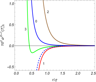
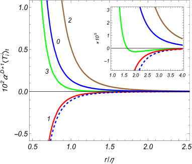
Figure 1: The radial dependence of the topological contributions in the vacuum energy-momentum tensor for spatial dimensions $D=5$ (left panel) and $D=6$ (right panel). The numbers near the curves correspond to the value of the index $i$ of the diagonal components $\langle T_{i}^{i}\rangle_{\mathrm{t}}$ and the graphs are plotted for $q=1.5$. The dashed curves present the energy flux $\langle T_{0}^{1}\rangle_{\mathrm{t}}$.

To show the dependence on the planar angle deficit, in Figures 2 and 3 we have presented the topological contributions in the diagonal components of the vacuum energy-momentum tensor, $10^{2}\alpha^{D+1}\langle T_{i}^{i}\rangle_{\mathrm{t}}$, as functions of the ratio $r/\eta$ and of the parameter $q$ for the spatial dimension $D=5$. The left and right panels of Figure 2 correspond to the energy density ($i=0$) and the radial stress ($i=1$), respectively. The left and right panels in Figure 3 present the azimuthal stress ($i=2$) and the axial stress ($i=3$). Depending on the values of $q$ and $r/\eta$, the energy density and the axial stress corresponding to the topological contributions can be either positive or negative. The radial azimuthal stresses are monotonic functions of both variables. These features are in agreement with the asymptotic analysis described above.

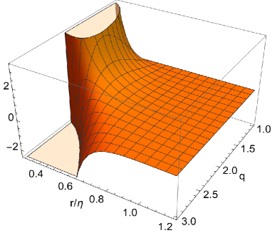
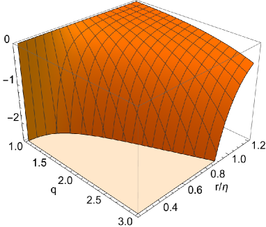
Figure 2: The topological contributions in the vacuum energy density, $10^{2}\alpha^{6}\langle T_{0}^{0}\rangle_{\mathrm{t}}$ (left panel), and in the radial stress, $10^{2}\alpha^{6}\langle T_{1}^{1}\rangle_{\mathrm{t}}$ (right panel), versus the proper distance from the cosmic string (in units of the curvature radius $\alpha$) and the parameter $q$ determining the planar angle deficit. The graphs are plotted for the model with $D=5$.

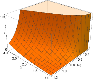
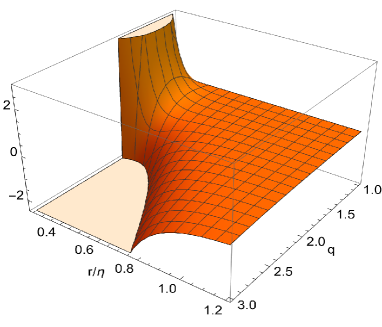
Figure 3: The same as in Figure 2 for the azimuthal stress $10^{2}\alpha^{6}\langle T_{2}^{2}\rangle_{\mathrm{t}}$ (left panel), and the axial stress $10^{2}\alpha^{6}\langle T_{3}^{3}\rangle_{\mathrm{t}}$ (right panel).

4 Energy flux

In the previous section we have investigated the diagonal components of the energy-momentum tensor. The problem under consideration is not homogeneous with respect to the coordinates $r$, $\eta$ and, in addition to the diagonal components, one has a nonzero off-diagonal component $\langle T_{0}^{1}\rangle$ that corresponds to the energy flux along the radial direction. The respective mode sum is obtained from (2.3) with the mode functions (2.9). Again, by using (3.1) for the summation over polarizations, one gets

$$\langle T_{0}^{1}\rangle=\frac{2i(D-3)q\eta^{D+2}}{(2\pi)^{D}\alpha^{D+1}}\partial_{r}\sideset{}{{}^{\prime}}{\sum}_{m=0}^{\infty}\int d\mathbf{k}\int_{0}^{\infty}d\gamma\,\omega\gamma K_{\frac{D}{2}-2}(\omega\eta e^{-\pi i/2})K_{\frac{D}{2}-1}(\omega\eta e^{\pi i/2})J_{qm}^{2}(\gamma r).$$ (4.1)

The radial derivative in the right-hand side excludes the contribution of the part corresponding to the dS geometry in the absence of the cosmic string. That part is zero as a consequence of the problem symmetry. The nonzero energy flux is a purely topological effect induced by the string. It is finite for $r>0$ and the cutoff function can be removed from the beginning.

For the further transformation of the energy flux we use the integral representation

$$K_{\nu-1}(e^{-i\pi/2}\omega\eta)K_{\nu}(e^{i\pi/2}\omega\eta) = -\frac{i}{2\eta\omega}\int_{-\infty}^{+\infty}dy\,e^{-2\nu y}\int_{0}^{\infty}\frac{dx}{x}\left(\nu-\frac{1}{x}\right)$$ (4.2)

$$\times\exp\left(-x\eta^{2}\omega^{2}\sinh^{2}y-\frac{1}{x}\right).$$

The latter is obtained from the representation [54]

$$K_{\nu}(e^{-i\pi/2}\omega\eta)K_{\nu}(e^{i\pi/2}\omega\eta^{\prime})=\frac{1}{2}\int_{-\infty}^{+\infty}dy\,e^{-2\nu y}\int_{0}^{\infty}\frac{du}{u}e^{-u/2-\omega^{2}\beta/(2u)},$$ (4.3)

with the notation $\beta=2\eta\eta^{\prime}\cosh(2y)-\eta^{2}-\eta^{\prime 2}$, taking the derivative with respect to the argument of the second Macdonald function in (4.3) and then passing to the limit $\eta^{\prime}\rightarrow\eta$. Substituting (4.2) (with $\nu=D/2-1$) into the expression (4.1), the integral over $\gamma$ is evaluated by using (3.10). After some transformations we find

$$\langle T_{0}^{1}\rangle_{\mathrm{t}} = \frac{(3-D)q\eta}{2\left(2\pi\right)^{D/2+1}\alpha^{D+1}}\int_{0}^{\infty}du\,u^{\frac{D}{2}-1}e^{u}K_{\frac{D}{2}-1}(u)$$ (4.4)

$$\times\partial_{r}\left(2+r\partial_{r}\right)e^{-u(r/\eta)^{2}}\sideset{}{{}^{\prime}}{\sum}_{m=0}^{\infty}I_{qm}(u(r/\eta)^{2}).$$

Next, by using the formula (3.15), one gets

$$\langle T_{0}^{1}\rangle_{\mathrm{t}}=\frac{8(D-3)r}{\left(2\pi\right)^{D/2+1}\alpha^{D+1}\eta}\left[\sum_{j=1}^{[q/2]}t^{(01)}(r/\eta,s_{j})-\frac{q}{\pi}\sin(q\pi)\int_{0}^{\infty}dy\frac{t^{(01)}(r/\eta,\cosh y)}{\cosh(2qy)-\cos(q\pi)}\right],$$ (4.5)

where the notation

$$t^{(01)}(x,y)=y^{2}\int_{0}^{\infty}du\,u^{\frac{D}{2}}\left(1-uy^{2}x^{2}\right)K_{\frac{D}{2}-1}(u)e^{u-2x^{2}y^{2}u},$$ (4.6)

has been used. Similar to the case of the diagonal components, the energy flux density $\langle T_{0}^{1}\rangle_{\mathrm{t}}$ depends on the radial and time coordinates through the ratio $r/\eta$ that presents to the proper distance from the cosmic string measured in units of the dS curvature radius $\alpha$. An equivalent expression for the function $t^{(01)}(x,y)$ is given by

$$t^{(01)}(x,y)=\frac{y^{2}}{2}\int_{0}^{\infty}du\,u^{\frac{D}{2}+1}e^{u-2x^{2}y^{2}u}\left[K_{\frac{D}{2}-2}(u)-K_{\frac{D}{2}-1}(u)\right].$$ (4.7)

This shows that this function is negative. For $\langle T_{0}^{1}\rangle_{\mathrm{t}}>0$ the energy flux is directed from the cosmic string and for $\langle T_{0}^{1}\rangle_{\mathrm{t}}<0$ it is directed towards the string.

As we could expect from the conformal relation with the problem of cosmic string in the Minkowski bulk, the energy flux vanishes for $D=3$. For other odd values of the spatial dimension $D$ the integral in  (4.6) is expressed in terms of the elementary functions. In particular, we get

$$\langle T_{0}^{1}\rangle_{\mathrm{t}}=-\frac{c_{4}(q)}{8\pi^{3}\alpha^{6}\left(r/\eta\right)^{5}},$$ (4.8)

for $D=5$ and

$$\langle T_{0}^{1}\rangle_{\mathrm{t}}=-\frac{3}{8}\frac{(r/\eta)^{2}c_{4}(q)+c_{6}(q)}{\pi^{4}\alpha^{8}(r/\eta)^{7}},$$ (4.9)

for $D=7$. In both these cases $\langle T_{0}^{1}\rangle_{\mathrm{t}}<0$.

For large values of the curvature radius, corresponding to the Minkowskian limit, the dominant contribution in the integral representation (4.6) for the function $t^{(01)}(r/\eta,y)$ comes from the integration range with large values of $u$. To the leading order we get

$$\langle T_{0}^{1}\rangle_{\mathrm{t}}\approx-\frac{\Gamma\left((D+1)/2\right)}{\left(4\pi\right)^{(D+1)/2}\alpha r^{D}}(D-3)^{2}c_{D-1}(q).$$ (4.10)

As we could expect, in the Minkowskian limit ($\alpha\rightarrow\infty$) the energy flux vanishes. The asymptotic of the energy flux near the cosmic string, corresponding to $r/\eta\ll 1$, is found in a similar way with the result

$$\langle T_{0}^{1}\rangle_{\mathrm{t}}\approx-\frac{(D-3)^{2}\Gamma\left((D+1)/2\right)}{\left(4\pi\right)^{(D+1)/2}\alpha^{D+1}\left(r/\eta\right)^{D}}c_{D-1}(q),\;r/\eta\ll 1.$$ (4.11)

In order to find the behavior of the energy flux at large distances from the string, $r/\eta\gg 1$, it is more convenient to use the representation (4.7) for the function $t^{(01)}(x,y)$. In the limit under consideration one has $x\gg 1$ and the main contribution to the integral in (4.7) gives the region near the lower limit. By using the asymptotics for the Macdonald function for small argument, we can see that, to the leading order,

$$\langle T_{0}^{1}\rangle_{\mathrm{t}}\approx-\frac{(D-3)\Gamma(D/2-1)c_{4}(q)}{8\pi^{D/2+1}\alpha^{D+1}\left(r/\eta\right)^{5}}.$$ (4.12)

In the special cases $D=5,7$ this result agrees with (4.8) and (4.9).

The asymptotic behavior of the energy flux for large values of $q$ is studied in the way similar to that we have used for the diagonal components. From (4.6), for $xy\gg 1$ we find

$$t^{(01)}(x,y)\approx\frac{\sqrt{\pi}\left(3-D\right)}{2^{D/2+3}x^{D+1}y^{D-1}}\Gamma\left(\frac{D+1}{2}\right).$$ (4.13)

In combination with (4.5) this gives the following leading term in the expansion over $1/q$:

$$\langle T_{0}^{1}\rangle_{\mathrm{t}}\approx-\frac{(D-3)^{2}\zeta\left(D-1\right)q^{D-1}}{2^{D+1}\pi^{3D/2-1/2}\alpha^{D+1}\left(r/\eta\right)^{D}}\Gamma\left(\frac{D+1}{2}\right).$$ (4.14)

By taking into account that $c_{n}(q)\approx\left(q/\pi\right)^{n}\zeta(n)$ for $q\gg 1$, in the special cases $D=5,7$ the general estimate (4.14) agrees with (4.8) and (4.9).

Figure 4 presents the energy flux versus the radial distance (left panel) and the parameter $q$ (right panel). The graphs on the left and right panels are plotted for $q=1.5$ and $r/\eta=1$, respectively. The numbers near the curves are the corresponding values of the spatial dimension. For all the cases $\langle T_{0}^{1}\rangle_{\mathrm{t}}<0$ and the energy flux is directed towards the cosmic string.

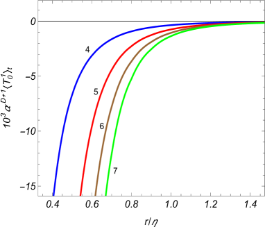
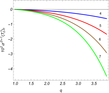
Figure 4: The energy flux as a function of the distance from the cosmic string (left panel) and as a function of the parameter $q$ (right panel). The left panel is plotted for $q=1.5$ and for the right panel we have taken $r/\eta=1$. The numbers near the curves present the values of the spatial dimension $D$.

As an additional check for the formulas given above we can show that the components of the topological contribution to the vacuum energy-momentum tensor obey the covariant conservation equation $\nabla_{i}\langle T_{l}^{i}\rangle_{\mathrm{t}}=0$. In the problem at hand two relations are obtained between the components corresponding to the equations with $l=0$ and $l=1$. By taking into account that all the components depend on $r$ and $\eta$ in the form of the ratio $w=r/\eta$, they are written as

$$\left(w\partial_{w}+D+1\right)\langle T_{0}^{0}\rangle_{\mathrm{t}} = -\left(\partial_{w}+\frac{1}{w}\right)\langle T_{0}^{1}\rangle_{\mathrm{t}}+\langle T_{i}^{i}\rangle_{\mathrm{t}},$$

$$\left(w\partial_{w}+D+1\right)\langle T_{0}^{1}\rangle_{\mathrm{t}} = \left(\partial_{w}+\frac{1}{w}\right)\langle T_{1}^{1}\rangle_{\mathrm{t}}-\frac{1}{w}\langle T_{2}^{2}\rangle_{t}.$$ (4.15)

With these relations, the components $\langle T_{i}^{i}\rangle_{t}$, $i=2,3,\ldots,D$, are expressed in terms of $\langle T_{0}^{0}\rangle_{t}$, $\langle T_{0}^{1}\rangle_{t}$, and $\langle T_{1}^{1}\rangle_{t}$. We recall that the components of the energy-momentum tensor were considered in the coordinate system $(\tau,r,\phi,\mathbf{z})$ with the conformal time $\tau$. For the components in the coordinates $(t,r,\phi,\mathbf{z})$, with $t$ being the synchronous time, one gets (no summation over $i$): $\langle T_{\mathrm{(s)}i}^{i}\rangle_{\mathrm{t}}=\langle T_{i}^{i}\rangle_{\mathrm{t}}$ and $\langle T_{\mathrm{(s)}0}^{1}\rangle_{\mathrm{t}}=e^{-t/\alpha}\langle T_{0}^{1}\rangle_{\mathrm{t}}$. The topological contribution in the vacuum energy contained in the spatial volume $V$ is expressed as $E_{V}^{\mathrm{(t)}}=\int_{V}d^{D}x\,e^{Dt/\alpha}\langle T_{\mathrm{(s)}0}^{0}\rangle_{\mathrm{t}}$. Taking the region $\{r_{1}\leq r\leq r_{2},\,0\leq\phi\leq\phi_{0},\,0\leq z^{i}\leq L_{i}\}$, $i=3,\ldots,D$, as the volume $V$, from the first equation (4.15) for the corresponding energy $E_{V}^{\mathrm{(t)}}=E_{r_{1}\leq r\leq r_{2}}^{\mathrm{(t)}}$ we get

$$\partial_{t}E_{r_{1}\leq r\leq r_{2}}^{\mathrm{(t)}}=\phi_{0}L_{3}\cdots L_{D}e^{Dt/\alpha}\left[-r\langle T_{\mathrm{(s)}0}^{1}\rangle_{\mathrm{t}}|_{r_{1}}^{r_{2}}+\frac{1}{\alpha}\int_{r_{1}}^{r_{2}}dr\,r\sum_{i=1}^{D}T_{i}^{i}\right].$$ (4.16)

By taking into account that $\phi_{0}r_{l}L_{3}\cdots L_{D}e^{(D-1)t/\alpha}$ is the proper surface area of the spatial hypersurface $\{r=r_{l},\,0\leq\phi\leq\phi_{0},\,0\leq z^{i}\leq L_{i}\}$, from (4.16) we see that $\langle T_{0}^{1}\rangle_{\mathrm{t}}$ is the energy flux per unit proper surface area. The second term in the square brackets of (4.16) corresponds to the work done by the vacuum stresses. We recall that for large $r$ the energy density $\langle T_{0}^{0}\rangle_{t}$ behaves as $1/r^{4}$ (with exception for the case $D=4$, see (3.56)) and, hence, the energy $E_{r_{1}\leq r\leq r_{2}}^{\mathrm{(t)}}$ is finite in the limit $r_{2}\rightarrow\infty$.

In the discussion above we have considered an idealized defect with zero thickness core. With this idealization, the topological contributions in the diagonal components diverge on the core as $1/r^{D+1}$ and the off-diagonal component behaves like $1/r^{D}$. Similar to the case of the Minkowskian bulk, discussed in [60], we can consider a simple model of finite core of radius $a$ with the interior geometry described by the nonsingular metric tensor $g_{il}=\left(\alpha/\tau\right)^{2}\mathrm{diag}(1,-1,-u^{2}(r),-1,\ldots,-1)$ for $r<a$. The geometry of the core is specified by the regular function $u(r)$. The exterior metric, $r>a$, as before, is given by (2.2). Matching of the interior and exterior geometries at $r=a$ is done by the Israel condition. This condition relates the derivative of the function $u(r)$ at $r=a$ with the surface energy-momentum tensor localized on the core boundary (see [60] for the Minkowski bulk). For the electromagnetic modes in the region $r>a$, instead of the Bessel function $J_{q|m|}(\gamma r)$, now the linear combination $J_{q|m|}(\gamma r)+b_{\beta}Y_{q|m|}(\gamma r)$, with the Neumann function $Y_{q|m|}(\gamma r)$, will appear. The coefficient $b_{\beta}$ is obtained from the matching conditions between the interior and exterior modes at $r=a$. In general, it will depend on the polarization and codifies the information about the interior geometry. The simplest model would be the core with perfectly reflecting boundary $r=a$ that induces the boundary condition $\left.n^{i}\,{}^{\ast}F_{ii_{1}\cdots i_{D-1}}\right|_{r=a}=0$, where $n^{i}$ is the normal vector of boundary and ${}^{\ast}F_{ii_{1}\cdots i_{D-1}}$ is the dual tensor for $F_{ik}$. For $D=3$ this corresponds to the boundary condition on the surface of a perfect conductor. The effects of a conducting cylindrical shell on the local characteristics of the electromagnetic vacuum in the geometry of a cosmic string in (3+1)-dimensional Minkowski bulk have been studied in [61]. The influence of a cylindrical boundary in $(D+1)$-dimensional dS spacetime, described by the line element (2.2) with $\phi_{0}=2\pi$ (the cosmic string is absent) on the VEVs of the sguared electric and magnetic fields and on the vacuum energy-momentum tensor is discussed in [45].

In the problem at hand, the effect of a perfectly reflecting finite core of the cosmic string on the vacuum energy-momentum tensor in the region $r>a$ can be investigated in the way similar to that used in [45] for the dS bulk without a cosmic string. The coefficient $b_{\beta}$ in the exterior mode functions is determined by the boundary condition at $r=a$. Convenient expressions for the finite core contributions in the VEVs are obtained by rotating the respective integrals over $\gamma$ in the complex plane (for the corresponding procedure see [45]). In this way the integrands are expressed in terms of the modified Bessel functions and the corresponding integrals exponentially converge in the upper limit for $r>a$. As a consequence, the vacuum energy-momentum tensor is decomposed as $\langle T_{i}^{l}\rangle=\langle T_{i}^{l}\rangle_{\mathrm{dS}}+\langle T_{i}^{l}\rangle_{\mathrm{t}}+\langle T_{i}^{l}\rangle_{\mathrm{fc}}$, where $\langle T_{i}^{l}\rangle_{\mathrm{dS}}$ is the VEV in dS spacetime, $\langle T_{i}^{l}\rangle_{\mathrm{t}}$ is the VEV considered in the discussion above, and $\langle T_{i}^{l}\rangle_{\mathrm{fc}}$ is the part induced by the finite core. When the angular deficit is absent, $\phi_{0}=2\pi$, at large distances from the core, $r/a,r/\eta\gg 1$, the boundary induced contribution $\langle T_{i}^{l}\rangle_{\mathrm{fc}}$ in spatial dimensions $D>4$ decays as [45] $1/[\left(r/\eta\right)^{D+2}\ln(r/a)]$ for the diagonal components and like $1/[\left(r/\eta\right)^{D+1}\ln(r/a)]$ for the component $\langle T_{0}^{1}\rangle_{\mathrm{fc}}$. For $D=4$ an additional factor $\ln(r/\eta)$ appears for the diagonal components. We expect a similar behavior in the presence of a cosmic string (the corresponding investigation will be presented elsewhere) and the part $\langle T_{i}^{l}\rangle_{\mathrm{t}}$ will be dominant compared to the contribution $\langle T_{i}^{l}\rangle_{\mathrm{fc}}$.

As it follows from the discussion above, the effects of cosmic string on the electromagnetic vacuum in spatial dimensions $D>3$ have qualitatively new features which are partially related to the absence of conformal invariance. These effects may have interesting implications in string theory motivated models where the role of cosmic strings is played by fundamental strings [62]. In those models the spatial dimension of the effective theory depends on the specific compactification scheme and may take values in the range $3\leq D\leq 9$. Another class of string theory inspired models with cosmic string type structures were discussed recently within the framework of brane inflationary models (see [21] for a review). The breakdown of conformal invariance for the electromagnetic field is required in inflationary models of the generation of large-scale magnetic fields from quantum fluctuations in the dS expansion stage (for the discussion of various mechanisms see, e.g., [17, 63, 64]). A possible mechanism, widely considered in the literature, is based on non-minimal interactions of the electromagnetic field with other fields. Another possibility, related to the dynamical evolution of extra spatial dimensions before a radiation-dominated epoch in models with $D>3$, has been discussed in [16]. If the preceding stage corresponds to the inflationary phase with dS expansion then the modifications of the electromagnetic vacuum fluctuations discussed above will be codified in large-scale perturbations of the magnetic field around the cosmic string in the post-inflationary epoch. An interesting signature for the presence of extra dimensions would be the energy flux in the radial direction (for features of inflationary models with cosmic strings see [19]). Several mechanisms have been discussed in the literature for the formation of cosmic strings during inflation [1]-[4]. They include the direct interaction between the inflaton and the field responsible for symmetry breaking, an additional coupling to the background curvature and quantum-mechanical tunnelling [65, 66, 67]. Among the interesting directions for the further research could be the back-reaction of the vacuum polarization we have discussed here on the spacetime geometry.

5 Conclusion

The expectation value of the energy-momentum tensor is among the central objects in quantum field theory on curved backgrounds. In addition to being an important local characteristic of a given state for quantum fields, it appears as a source of the gravitational field in semiclassical Einstein equations and determines the back reaction effects of quantum matter on the spacetime geometry. We have discussed the combined effects of the background geometry and topology on the VEV of the energy-momentum tensor for the electromagnetic field in $(D+1)$-dimensional locally dS spacetime. The nontrivial topology is generated by the presence of a topological defect that is a generalization of a cosmic string in 4-dimensional spacetime. The corresponding geometry is described by the line element (2.2) where the information on the defect is codified in the angle deficit $2\pi-\phi_{0}$.

For evaluation of the VEV of the energy-momentum tensor we have employed the mode-sum formula (2.3), with the mode functions for the vector potential given by (2.9). The regularization of the mode-sum is done by introducing the cutoff function $e^{-b\omega^{2}}$. The application of the formula (3.15) allowed us to extract from the expectation values the contributions corresponding to the pure dS bulk when the cosmic string is absent. For spacetime points outside the defect core, $r>0$, the presence of the cosmic string does not alter the local geometry and, hence, does not induce new divergences in the vacuum energy-momentum tensor compared to those for dS spacetime. Consequently, the topological contributions in the VEVs are finite for $r>0$ and the regularization in the corresponding expressions can be directly removed passing to the limit $b\rightarrow 0$ for the parameter in the cutoff function. The diagonal components of the topological contribution to the VEV of the energy-momentum tensor are given by (3.18), where the function $t^{(i)}(x,y)$ is defined as (3.19), or equivalently, as (3.22). An additional nonzero off-diagonal component of the vacuum energy-momentum tensor, describing energy flux along the radial direction, is given by the expression (4.5) with two equivalent expressions, (4.6) and (4.7), for the function $t^{(01)}(x,y)$ in the integrand. Because of the maximal symmetry of dS spacetime, the VEVs depend on the time and radial coordinates in terms of the proper radial distance form the cosmic string core, given by the combination $\alpha r/\eta=re^{t/\alpha}$. For the topological contributions we have explicitly checked the trace relation (3.35) and the covariant conservation equation. In the problem at hand the latter is reduced to the set of equations (4.15).

To clarify the dependence of the topological terms on the parameters of the problem special cases and asymptotic regions have been considered. In the limit $\alpha\rightarrow\infty$ with fixed $t$, from the expressions for the diagonal components of the energy-momentum tensor in dS spacetime the cosmic string induced vacuum energy-momentum tensor is obtained in the Minkowski bulk. In this special case the stresses along the directions parallel to the core of the defect are equal to the energy density and they are given by (3.47), whereas the radial and azimuthal components are expressed as (3.48). All the components are monotonic functions of the radial coordinate with power law decay $1/r^{D+1}$. The off-diagonal component vanishes in the Minkowskian limit. The leading term in the corresponding expansion over $1/\alpha$ is expressed as (4.10). The electromagnetic field is conformally invariant in 4-dimensional dS spacetime and the corresponding topological contributions are obtained from the expressions in the Minkowski bulk with the radial coordinate replaced by the proper distance from the string $\alpha r/\eta$. For odd values of the spatial dimension $D$ the expressions for the topological terms in dS bulk are further simplified by evaluating the integrals in (3.22) and (4.7). The corresponding VEVs are expressed in terms of the functions (3.40) with even values of the index $n$. Those functions are polynomials of degree $n$ (see (3.41), (3.46)).

For points near the cosmic string, corresponding to small proper distances compared to the curvature radius of dS spacetime, the influence of the gravitational field on the diagonal components of the topological terms is weak. The leading terms in the expansion over $r/\eta$ coincide with the corresponding results in the Minkowski bulk where the radial distance is replace by the proper distance $\alpha r/\eta$. The energy flux along the radial direction is an effect induced by the gravity and the asymptotic of the corresponding component of the energy-momentum tensor near the cosmic string is given by (4.11). The effects of gravity on the topological contributions in the VEV of the energy-momentum tensor are essential at proper distances from the cosmic string larger than the dS curvature radius. For $r/\eta\gg 1$ and $D\geq 4$ the corresponding asymptotic for the diagonal components is given by (3.55). The exception is the energy density for $D=4$ with the asymptotic behavior (3.56). For the energy flux density the decay at large distances is stronger, like $1/\left(r/\eta\right)^{5}$. Note that in contrast to the problem of cosmic string in the Minkowski bulk, for dS background geometry the degree of power law decay of the topological contributions at large distances does not depend on the spatial dimension.

References

- [1] A. Vilenkin, E.P.S. Shellard, Cosmic Strings and Other Topological Defects (Cambridge University Press, Cambridge, UK, 2000).
- [2] M.B. Hindmarsh, T.W.B. Kibble, Cosmic strings, Rep. Prog. Phys. 58, 411–562 (1995).
- [3] M. Sakellariadou, Cosmic strings, Lecture Notes in Physics, vol. 718, 247–288 (2007).
- [4] E.J. Copeland, T.W.B. Kibble, Cosmic strings and superstrings, Proc. Roy. Soc. Lond. A466, 623–657 (2010).
- [5] C. Ringeval, Cosmic strings and their induced non-Gaussianities in the cosmic microwave background, Adv. Astron. 2010, 380507 (2010).
- [6] A.D. Linde, Particle Physics and Inflationary Cosmology (Harwood Academic Publishers, Chur, Switzerland, 1990).
- [7] B.A. Bassett, S. Tsujikawa, D. Wands, Inflation dynamics and reheating, Rev. Mod. Phys. 78, 537–589 (2007).
- [8] J. Martin, C. Ringeval, V. Vennin, Encyclopedia Inflationaris, Phys. Dark Univ. 5-6, 75–235 (2014).
- [9] A.G. Riess, et al., Observational evidence from supernovae for an accelerating universe and a cosmological constant, Astron. J. 116, 1009–1038 (1998).
- [10] S. Perlmutter, et al., Measurements of omega and lambda from 42 high-redshift supernovae, Astrophys. J. 517, 565–586 (1999).
- [11] A.G. Riess, et al., New Hubble space telescope discoveries of Type Ia supernovae at : Narrowing constraints on the early behavior of dark energy, Astrophys. J. 659, 98–121 (2007).
- [12] D.N. Spergel, et al., Three-year Wilkinson Microwave Anisotropy Probe (WMAP) observations: Implications for cosmology, Astrophys. J. Suppl. Ser. 170, 377–408 (2007).
- [13] E. Komatsu, et al., Five-year Wilkinson Microwave Anisotropy Probe (WMAP) observations: Cosmological interpretation, Astrophys. J. Suppl. Ser. 180, 330–376 (2009).
- [14] D.H. Weinberg, et al., Observational probes of cosmic acceleration, Phys. Rep. 530, 87–255 (2013).
- [15] P.A.R. Ade, et al., Planck 2013 results. XVI. Cosmological parameters, A&A 571, A16 (2014).
- [16] M. Giovannini, Magnetogenesis and the dynamics of internal dimensions, Phys. Rev. D 62, 123505 (2000).
- [17] M. Giovannini, The magnetized universe, Int. J. Mod. Phys. D 13, 391-502 (2004).
- [18] K. Atmjeet, I. Pahwa, T.R. Seshadri, K. Subramanian, Cosmological magnetogenesis from extra-dimensional Gauss-Bonnet gravity, Phys. Rev. D 89, 063002 (2014).
- [19] M. Hindmarsh, Signals of inflationary models with cosmic strings, Prog. Theor. Phys. Suppl. 190, 197–228 (2011).
- [20] E.J. Copeland, L. Pogosian, T. Vachaspati, Seeking string theory in the cosmos, Class. Quantum Grav. 28, 204009 (2011).
- [21] D.F. Chernoff, S.-H. Henry Tye, Inflation, string theory and cosmic strings, Int. J. Mod. Phys. D 24, 1530010 (2015).
- [22] A.M. Ghezelbash, R.B. Mann, Vortices in de Sitter spacetimes, Phys. Lett. B 537, 329-339 (2002).
- [23] A.H. Abbassi, A.M. Abbassi, H. Razmi, Cosmological constant influence on cosmic string spacetime, Phys. Rev. D 67, 103504 (2003).
- [24] E.R. Bezerra de Mello, Y. Brihaye, B. Hartmann, Strings in de Sitter space, Phys. Rev. D 67, 124008 (2003).
- [25] J. Podolský, J.B. Griffiths, A snapping cosmic string in a de Sitter or anti-de Sitter universe, Class. Quantum Grav. 21, 2537-2547 (2004).
- [26] Y. Brihaye, B. Hartmann, Cosmic strings in a space-time with positive cosmological constant, Phys. Lett. B 669, 119-125 (2008).
- [27] A. de Pádua Santos, E. R. Bezerra de Mello, Non-Abelian cosmic strings in de Sitter and anti-de Sitter space, Phys. Rev. D 94, 063524 (2016).
- [28] P.C.W. Davies, V. Sahni, Quantum gravitational effects near cosmic strings, Class. Quantum Grav. 5, 1 (1988).
- [29] E.R. Bezerra de Mello, A.A. Saharian, Vacuum polarization by a cosmic string in de Sitter spacetime, J. High Energy Phys. JHEP04(2009)046.
- [30] E.R. Bezerra de Mello, A.A. Saharian, Fermionic vacuum polarization by a cosmic string in de Sitter spacetime, J. High Energy Phys. JHEP08(2010)038.
- [31] A.A. Saharian, V.F. Manukyan, N.A. Saharyan, Electromagnetic vacuum fluctuations around a cosmic string in de Sitter spacetime, Eur. Phys. J. C 77, 478 (2017).
- [32] A.A. Saharian, V.F. Manukyan, N.A. Saharyan, Electromagnetic vacuum densities induced by a cosmic string. Paricles 1, 13 (2018).
- [33] A. Mohammadi, E.R. Bezerra de Mello, A.A. Saharian, Induced fermionic currents in de Sitter spacetime in the presence of a compactified cosmic string, Class. Quantum Grav. 32, 135002 (2015).
- [34] E.A.F. Bragança, E.R. Bezerra de Mello, A. Mohammadi, Induced fermionic vacuum polarization in a de Sitter spacetime with a compactified cosmic string, Phys. Rev. D 101, 045019 (2020).
- [35] E.A.F. Bragança, E.R. Bezerra de Mello, A. Mohammadi, Vacuum bosonic currents induced by a compactified cosmic string in dS background, Int. J. Mod. Phys. D 29, 2050103 (2020).
- [36] E.R. Bezerra de Mello, A.A. Saharian, Vacuum polarization induced by a cosmic string in anti-de Sitter spacetime, J. Phys. A 45, 115002 (2012).
- [37] E.R. Bezerra de Mello, E.R. Figueiredo Medeiros, A.A. Saharian, Fermionic vacuum polarization by a cosmic string in anti-de Sitter spacetime, Classical Quantum Gravity 30, 175001 (2013).
- [38] W. Oliveira dos Santos, H.F. Santana Mota, E.R. Bezerra de Mello, Induced current in high-dimensional AdS spacetime in the presence of a cosmic string and a compactified extra dimension, Phys. Rev. D 99, 045005 (2019).
- [39] W. Oliveira dos Santos, E.R. Bezerra de Mello, H. F. Mota, Vacuum polarization in high-dimensional AdS spacetime in the presence of a cosmic string and a compactified extra dimension, Eur. Phys. J. Plus 135, 27 (2020).
- [40] S. Bellucci, W. Oliveira dos Santos, E.R. Bezerra de Mello, Induced fermionic current in AdS spacetime in the presence of a cosmic string and a compactified dimension, Eur. Phys. J. C 80, 963 (2020).
- [41] S. Bellucci, W. Oliveira dos Santos, E. R. B. de Mello, A. A. Saharian, Topological effects in fermion condensate induced by cosmic string and compactification on AdS bulk, Symmetry 14, 584 (2022).
- [42] S. Bellucci, W. Oliveira dos Santos, E. R. Bezerra de Mello, A. A. Saharian, Fermionic vacuum polarization around a cosmic string in compactified AdS spacetime, J. Cosmol. Astropart. Phys. 01 (2022) 010.
- [43] S. Bellucci, W. Oliveira dos Santos, E. R. Bezerra de Mello, A. A. Saharian, Cosmic string and brane induced effects on the fermionic vacuum in AdS spacetime, J. High Energy Phys. JHEP05(2022)021.
- [44] E.R. Bezerra de Mello, W. Oliveira dos Santos, A.A. Saharian, Finite temperature charge and current densities around a cosmic string in AdS spacetime with compact dimension, Phys. Rev. D 106, 125009 (2022).
- [45] A.A. Saharian, V.F. Manukyan, N.A. Saharyan, Electromagnetic Casimir densities for a cylindrical shell on de Sitter space, Int, J. Mod. Phys. A 31, 1650183 (2016).
- [46] B. Allen, T. Jacobson, Vector two-point functions in maximally symmetric spaces, Commun. Math. Phys. 103, 669-692 (1986).
- [47] N.C. Tsamis, R.P. Woodard, A maximally symmetric vector propagator, J. Math. Phys. 48, 052306 (2007).
- [48] A. Higuchi, Y.C. Lee, J.R. Nicholas, More on the covariant retarded Green’s function for the electromagnetic field in de Sitter spacetime. Phys. Rev. D 80, 107502 (2009).
- [49] A. Youssef, Infrared behavior and gauge artifacts in de Sitter spacetime: The photon field, Phys. Rev. Lett. 107, 021101 (2011).
- [50] M.B. Fröb, A. Higuchi, Mode-sum construction of the two-point functions for the Stueckelberg vector fields in the Poincaré patch of de Sitter space, J. Math. Phys. 55, 062301 (2014).
- [51] S. Domazet, T. Prokopec, A photon propagator on de Sitter in covariant gauges, arXiv:1401.4329.
- [52] G. Narain, Green’s function of the vector fields on de Sitter background, arXiv:1408.6193.
- [53] D. Glavan, T. Prokopec, Photon propagator in de Sitter space in the general covariant gauge, arXiv:2212.13982.
- [54] G.N. Watson, A Treatise on the Theory of Bessel Functions (Cambridge University Press, Cambridge, UK, 1966).
- [55] A.P. Prudnikov, Yu.A. Brychkov, O.I. Marichev, Integrals and Series (Gordon and Breach, New York, 1986), Vol. II.
- [56] E.R. Bezerra de Mello, V.B. Bezerra, A.A. Saharian, V.M. Bardeghyan, Fermionic current densities induced by magnetic flux in a conical space with a circular boundary, Phys. Rev. D 82, 085033 (2010).
- [57] E.R. Bezerra de Mello, V.B. Bezerra, A.A. Saharian, A.S. Tarloyan, Vacuum polarization induced by a cylindrical boundary in the cosmic string spacetime, Phys. Rev. D 74, 025017 (2006).
- [58] V.P. Frolov, E.M. Serebriany, Vacuum polarization in the gravitational field of a cosmic string, Phys. Rev. D 35, 3779-3782 (1987).
- [59] J.S. Dowker, Vacuum averages for arbitrary spin around a cosmic string, Phys. Rev. D 36, 3742-3746 (1987).
- [60] E.R. Bezerra de Mello, V.B. Bezerra, A.A. Saharian, H.H. Harutyunyan, Vacuum currents induced by a magnetic flux around a cosmic string with finite core, Phys. Rev. D 91, 064034 (2015).
- [61] E.R. Bezerra de Mello, V.B. Bezerra, A.A. Saharian, Electromagnetic Casimir densities induced by a conducting cylindrical shell in the cosmic string spacetime, Phys. Lett. B645, 245-254 (2007).
- [62] E. Witten, Cosmic superstrings, Phys. Lett. B153, 243-245 (1985)
- [63] A. Kandusa, K.E. Kunze, C.G. Tsagas, Primordial magnetogenesis, Phys. Rep. 505, 1-58 (2011).
- [64] R. Durrer, A. Neronov, Cosmological magnetic fields: their generation, evolution and observation, Astron. Astrophys. Rev. 21, 62-109 (2013).
- [65] N. Turok, String driven inflation, Phys. Rev. Lett. 60, 549-552 (1988).
- [66] R. Basu, A.H. Guth, A. Vilenkin, Quantum creation of topological defects during inflation, Phys. Rev. D 44, 340-351 (1991).
- [67] G. Lazarides, R. Maji, Q. Shafi, Cosmic strings, inflation, and gravity waves, Phys. Rev. D 104, 095004 (2021).