Adjoint Method in PDE-based Image Compression

Abstract

We consider a shape optimization based method for finding the best interpolation data in the compression of images with noise. The aim is to reconstruct missing regions by means of minimizing a data fitting term in an $L^{p}$-norm between original images and their reconstructed counterparts using linear diffusion PDE-based inpainting. Reformulating the problem as a constrained optimization over sets (shapes), we derive the topological asymptotic expansion of the considered shape functionals with respect to the insertion of small ball (a single pixel) using the adjoint method. Based on the achieved distributed topological shape derivatives, we propose a numerical approach to determine the optimal set and present numerical experiments showing, the efficiency of our method. Numerical computations are presented that confirm the usefulness of our theoretical findings for PDE-based image compression.

Keywords image compression  $\cdot$ shape optimization  $\cdot$ adjoint method  $\cdot$ image interpolation  $\cdot$ inpainting  $\cdot$ PDEs  $\cdot$ image denoising

Introduction and Related Works

PDE-based methods have attracted growing interest by researchers and engineers in image analysis field during the last decades [23, 9, 28, 18, 29, 8, 25, 17, 16, 1]. Actually, such methods have reached their maturity both from the point of view of modeling and scientific computing allowing them to be used in modern image technologies and their various applications. Image compression is one of the domain where they appear among the state-of-the-art methods [11, 13, 26, 4, 24, 3, 19]. In fact, the aim for such problems is to store few pixels of a given image (coding phase) and to recover/restore the missing part in an accurate way (decoding). The PDE-based methods use a diffusion differential operator for the inpainting of missed parts from a available data (boundary or small parts of the initial image) therefore their efficiency for decoding is guaranteed/encoded in the operator without any pre- or post-treatment. The question then is how to ensure with these methods a good choice, if it exists, of the “best” pixels to store for high quality reconstruction of the entire image? An answer to this question is given in [6, 7] for the harmonic or the heat equation, where its reformulation as a constrained (shape) optimisation problem permitted to exhibit an optimal set of pixels to do the job. In addition, analytic selection criteria using topological asymptotics were derived. Due to the simple structure of the shape functionals considered in these previous works, the topological expansion is easily derived (more or less with formal computations) and gives an analytic criterion to characterize the optimal set in compression. The limitation in obtaining the topological expansion this way is twofold : the criterion gives pointwise information on the importance of the location (pixel) to store which results in hard thresholding selection strategy not robust with respect to the noise. Second, the technique is limited to simple functionals, namely an $L^{2}$ data-fitting term and a linear diffusion operator.

The main contribution of this article is the use of the adjoint methods to derive a soft analytic criterion for PDE-based compression. Though we restrict our selves to second order linear inpainting, the method applies without significant changes to more general elliptic operators and as we show in the article to several type of noise.

In fact, we consider the compression problem in the same framework than [6], but we introduce a new approach to the characterization of the set of pixels to store using the adjoint method [15, 14, 2, 5]. This approach to obtain the topological expansion is more general than the one previously studied for the same problem, in the sense that it may be used for other diffusion operators and nonlinear data-fitting term, moreover it allows a better stability with respect to noise for the selection criteria. In particular, when the accuracy of the reconstruction (fidelity term) is measured with an $L^{p}$-norm, $p>1$ and $p\not=2$, the adjoint problem is still linear and no further complexity is added to the considered problem. Thus, the main results in the article include the rigorous derivation of the topological expansion based on the adjoint problem. We notice that the Dirichlet boundary in the inclusion prevents from a direct transposition of the adjoint method based on a local perturbation of the material properties by insertion of a hole. Therefore, we extend the sensibility analysis to the problem under consideration and we perform the asymptotic expansion of the proposed shape functional using non-standard perturbation techniques combined with truncation techniques. The asymptotic allows us to deduce a gradient algorithm for the reconstruction.

The article is organized as follows : in Section 1, we introduce the compression problem that takes the form of a constrained optimization problem of finding the best set of pixels to store, denoted $K$. Section 2 is devoted to describe the adjoint method to compute the topological derivative of the cost functional considered. In Section 3, we perform the computations to obtain the topological expansion and the “shape” derivatives which involve the direct and adjoint states. Finally, in Section 4, we describe the resulting algorithm and we give some numerical results to confirm the usefulness of the theory. Some of the technical proofs and auxiliary estimates are given in appendices for ease of readability.

1 Problem Formulation

Let $D\subset\mathbb{R}^{2}$ and $f:D\to\mathbb{R}^{d}$, $d\geq 1$ a given image in some region $K\subset\subset D$. We consider the mixed elliptic boundary problem for a given $u_{0}$ in $L^{2}(D)$,

Problem 1.1.

Find $u$ in $H^{1}(D)$ such that

$$\left\{\begin{array}[]{rl}u-\alpha\Delta u=u_{0},&\text{in}\ D\setminus K,\\ u=f,&\text{in}\ K,\\ \frac{\partial u}{\partial\mathbf{n}}=0,&\text{on}\ \partial D.\\ \end{array}\right.$$ (1)

where the available data $f$ is a Dirichlet “boundary” condition and with homogeneous Neumann boundary condition on $\partial D$. This PDE corresponds to the first term in the time discretization of the homogeneous heat equation, where we assume that the initial condition is $u_{0}$. For compatibility condition with the “boundary” data on $K$, we take as $u_{0}$ the image $f\in H^{1}(D)$, with $\Delta f\in L^{2}(D)$ and such that $\frac{\partial f}{\partial n}=0$ on $\partial D$. Setting $v=u-f$, we can write equivalently

Problem 1.2.

Find $v$ in $H^{1}(D)$ such that

$$\left\{\begin{array}[]{rl}v-\alpha\Delta v=\alpha\Delta f,&\text{in}\ D\setminus K,\\ v=0,&\text{in}\ K,\\ \frac{\partial v}{\partial\mathbf{n}}=0,&\text{on}\ \partial D.\\ \end{array}\right.$$ (2)

Denoting by $v_{K}=u_{K}-f$ the solution of Problem 2, the question is to identify the region $K$ which gives the “best” approximation $u_{K}$, in a suitable sense, that is to say which minimizes some $L^{p}$-norm. The constrained optimization problem for the compression reads [6], for $p>1$,

$$\min_{K\subseteq D,\ m(K)\leq c}\Big{\{}\frac{1}{p}\int_{D}|u_{K}-f|^{p}\ dx\ \Big{|}\ u_{K}\ \text{solution of Problem}\ \ref{pb:problem_1}\Big{\}},$$ (3)

where $m$ is a “size measure". The optimization problem (3) is studied in [6] and the existence of an optimal set is established for $p=2$ and $m$ is the capacity of sets [30] and the result extends to $p>1$ as noticed in [7]. The optimal set $K$ is obtained via a relaxation procedure but its regularity is not considered yet, nevertheless the relaxation technique allows us to derive first order optimality conditions via topological derivatives, which was done in [6] in the case of the Laplacian as inpainting operator. In this article, we aim to compute the topological gradient [10, 2] of the shape functional using the adjoint method which possesses two main advantages on the previous approaches: it is more general and systematic with respect to the inpainting operator and the exponent $p\geq 1$, on one side and secondly, it leads to a better characterization of the relevant pixels as it gives a distribution of such pixels taking into account local informations from their neighborhood. Loosely speaking, to obtain the topological derivative, let $x_{0}\in D$ and $K_{\varepsilon}=K\cup\overline{B(x_{0},\varepsilon)}$ ($B(x_{0},\epsilon)$ denotes the ball centred at $x_{0}$ with radius $\varepsilon$), then we look for an expansion of the form

$$J(u_{K_{\varepsilon}})-J(u_{K})=\rho(\varepsilon)\,G(x_{0})+o\big{(}\rho(\varepsilon)\big{)}.$$

where $\rho$ is a positive function going to zero with $\varepsilon$ and $G$ is the so called topological gradient [2, 5, 14]. Therefore, to minimize the cost functional $J$, one has to create small holes at the locations $x$ where $G(x)$ is the most negative. For the compression problem this amount to select the locations where the pixels are the most important to keep.

2 Adjoint Method and variations of the cost functional

We introduce the following abstract result which describes an adjoint method for the computation of the first variation of a given cost functional (see for instance [2]). Let $V$ be a Hilbert space. We recall the involved norms in Appendix A.1. For $\varepsilon\in[0,\zeta]$, $\zeta>0$, we consider a symmetric bilinear form $a_{\varepsilon}:V\times V\to\mathbb{R}$ and a linear form $l_{\varepsilon}:V\to\mathbb{R}$ such that the following assumptions are fulfilled

• $|a_{\varepsilon}(v,w)|\leq M_{1}\|v\|\|w\|$, $\forall(v,w)\in V\times V$ (continuity of the bilinear form),

• $a_{\varepsilon}(v,v)\geq\alpha\|v\|^{2}$, $\forall v\in V$ (uniform coercivity),

• $|l_{\varepsilon}(w)|\leq M_{2}\|w\|$, $\forall w\in V$ (continuity of the linear form),

with $\alpha,M_{1},M_{2}>0$ independent of $\varepsilon$. Moreover, we suppose that there exists a continuous bilinear form $\delta a:V\times V\to\mathbb{R}$, a continuous linear form $\delta l:V\to\mathbb{R}$ and a function $\rho:\mathbb{R}_{+}\to\mathbb{R}_{+}$ such that, for all $\varepsilon\geq 0$,

• $\|a_{\varepsilon}-a_{0}-\rho(\varepsilon)\,\delta a\|_{\mathcal{L}_{2}(V)}=o\big{(}\rho(\varepsilon)\big{)}$,

• $\|l_{\varepsilon}-l_{0}-\rho(\varepsilon)\,\delta l\|_{\mathcal{L}(V)}=o\big{(}\rho(\varepsilon)\big{)}$,

• $\lim_{\varepsilon\to 0}\rho(\varepsilon)=0$.

We emphasis that $\delta a$ and $\delta l$ do not depend on $\varepsilon$. Finally, for all $\varepsilon\in[0,\zeta]$, consider a functional $J_{\varepsilon}:V\to\mathbb{R}$, Fréchet-differentiable at the point $v_{0}$. Assume further that there exists a number $\delta J(v_{0})$ such that

$$J_{\varepsilon}(w)-J_{0}(v)=DJ_{0}(v)(w-v)+\rho(\varepsilon)\,\delta J(v)+o\big{(}\|w-v\|+\rho(\varepsilon)\big{)},\ \forall(v,w)\in V\times V.$$

Then we have [2]

Theorem 2.1.

Let $v_{\varepsilon}\in V$ be the solution of the following problem : find $v\in V$ such that,

$$a_{\varepsilon}(v,\varphi)=l_{\varepsilon}(\varphi),\ \forall\varphi\in V.$$

Let $w_{0}$ be the solution of the so-called adjoint problem : find $w\in V$ such that

$$a_{0}(w,\varphi)=-DJ_{0}(v_{0})\varphi,\ \forall\varphi\in V.$$

Then,

$$J_{\varepsilon}(v_{\varepsilon})-J_{0}(v_{0})=\rho(\varepsilon)\big{(}\delta a(v_{0},w_{0})-\delta l(w_{0})+\delta J(v_{0})\big{)}+o\big{(}\rho(\varepsilon)\big{)}.$$

To be more specific, for $x_{0}\in D$ and $r>0$, we denote by $B_{r}$ the open ball centred at $x_{0}$ and of radius $r$. We set

$$V_{\varepsilon}:=\{v\in H^{1}(D\setminus B_{\varepsilon})\ |\ v=0\ \text{on}\ \partial B_{\varepsilon}\}.$$

Then we consider the boundary value problem :

Problem 2.1.

Find $\widetilde{v}_{\varepsilon}$ in $V_{\varepsilon}$ such that

$$\left\{\begin{array}[]{cl}-\alpha\Delta\widetilde{v}_{\varepsilon}+\widetilde{v}_{\varepsilon}=h,&\text{in}\ D\setminus B_{\varepsilon},\\ \widetilde{v}_{\varepsilon}=0,&\text{in}\ B_{\varepsilon},\\ \partial_{n}\widetilde{v}_{\varepsilon}=0,&\text{on}\ \partial D.\end{array}\right.$$ (4)

with $h:=\alpha\Delta f$, but $h$ can be any $L^{2}(D)$ function. We denote $\widetilde{v}_{0}$ the solution of the problem

Problem 2.2.

Find $\widetilde{v}_{0}$ in $H^{1}(D)$ such that

$$\left\{\begin{array}[]{cl}-\alpha\Delta\widetilde{v}_{0}+\widetilde{v}_{0}=h,&\text{in}\ D,\\ \partial_{n}\widetilde{v}_{0}=0,&\text{on}\ \partial D.\end{array}\right.$$ (5)

The weak formulation of problems below reads, find $\widetilde{v}_{\varepsilon}$ in $V_{\varepsilon}$ such that, for all $\varphi$ in $V_{\varepsilon}\cap H^{1}(D)$, we have

$$\tilde{a}_{\varepsilon}(\widetilde{v}_{\varepsilon},\varphi)=\tilde{l}_{\varepsilon}(\varphi),$$

with,

$$\tilde{a}_{\varepsilon}(\widetilde{v}_{\varepsilon},\varphi):=\alpha\int_{D\setminus B_{\varepsilon}}\nabla\widetilde{v}_{\varepsilon}\cdot\nabla\varphi\ dx+\int_{D\setminus B_{\varepsilon}}\widetilde{v}_{\varepsilon}\,\varphi\ dx,$$

$$\tilde{l}_{\varepsilon}(\varphi):=\int_{D\setminus B_{\varepsilon}}h\,\varphi\ dx.$$

The dependency of the space $V_{\varepsilon}$ on $\varepsilon$ prevents us from using Theorem 2.1 directly, therefore, we introduce a truncation technique [15], which consists of inserting a ball $B_{R}$, for a fixed $R>\zeta$ and splitting Problem 4 into two sub-problems that we glue at their common boundary (see Figure 1). More precisely, we consider the sub-problems : an internal problem

$$\left\{\begin{array}[]{cl}-\alpha\Delta v_{\varepsilon,R}+v_{\varepsilon,R}=h,&\text{in}\ B_{R}\setminus B_{\varepsilon},\\ v_{\varepsilon,R}=0,&\text{on}\ \partial B_{\varepsilon},\\ v_{\varepsilon,R}=v_{\varepsilon},&\text{on}\ \partial B_{R},\end{array}\right.$$

and an external problem

$$\left\{\begin{array}[]{cl}-\alpha\Delta v_{\varepsilon}+v_{\varepsilon}=h,&\text{in}\ D\setminus B_{R},\\ \partial_{n}v_{\varepsilon}=\partial_{n}v_{\varepsilon,R},&\text{on}\ \partial B_{R},\\ \partial_{n}v_{\varepsilon}=0,&\text{on}\ \partial D.\end{array}\right.$$

[scale=0.35]

[fill=black!10] (-6.75, 15) .. controls + (-1,-0.5) and + (1,1.5) .. (-12.5, 10.75) .. controls + (-1,-1.5) and + (-0.5,1.5) .. (-13.25, 0) .. controls + (0.5,-1.5) and + (-3,-1) .. (-5, 4.75) .. controls + (3,1) and + (1,-2) .. (5, 7.25) .. controls + (-1,2) and + (2,-1) .. (-2.75, 14.75) .. controls + (-2,1) and + (1,0.5) .. (-6.75, 15) – cycle;

(6) at (-11,3.5) $D\setminus B_{\varepsilon}$;

[circle, draw=black, fill=white, inner sep=0pt,minimum size=25pt] (1) at (-5,10) $B_{\varepsilon}$;

[->] (-13,14) – (-10,10);

(3) at (-13.5,14.5) $\widetilde{v}_{\varepsilon}$;

(a) Before splitting.

[scale=0.35]

[fill=black!10] (-6.75, 15) .. controls + (-1,-0.5) and + (1,1.5) .. (-12.5, 10.75) .. controls + (-1,-1.5) and + (-0.5,1.5) .. (-13.25, 0) .. controls + (0.5,-1.5) and + (-3,-1) .. (-5, 4.75) .. controls + (3,1) and + (1,-2) .. (5, 7.25) .. controls + (-1,2) and + (2,-1) .. (-2.75, 14.75) .. controls + (-2,1) and + (1,0.5) .. (-6.75, 15) – cycle;

(6) at (-11,3.5) $D\setminus B_{R}$;

[circle, dashed, draw=black, fill=black!25, inner sep=0pt,minimum size=70pt] (1) at (-5,10) ; (6) at (-5,7.8) $B_{R}\setminus B_{\varepsilon}$; [circle, draw=black, fill=white, inner sep=0pt,minimum size=25pt] (2) at (-5,10) $B_{\varepsilon}$;

[->] (-13,14) – (-10,10); (3) at (-13.5,14.5) $v_{\varepsilon}$; [->] (1,14) – (-2.8,11); (3) at (1.5,14.5) $v_{\varepsilon,R}$;

(b) After splitting.

Figure 1: Illustration of the splitting.

As the two sub-problems transform the initial one into a transmission problem. We have

Proposition 2.1.

We have,

$$\widetilde{v}_{\varepsilon}=\begin{cases}v_{\varepsilon},&\text{in}\ D\setminus B_{R},\\ v_{\varepsilon,R},&\text{in}\ B_{R}\setminus B_{\varepsilon}.\end{cases}$$

Proof.

We set

$$v:=\begin{cases}v_{\varepsilon}&,\ \text{in}\ D\setminus B_{R},\\ v_{\varepsilon,R}&,\ \text{in}\ B_{R}\setminus B_{\varepsilon}.\end{cases}$$ (6)

Let $\varphi$ be in $V_{\varepsilon}$, then,

$$\tilde{a}_{\varepsilon}(v,\varphi) =\alpha\int_{D\setminus B_{R}}\nabla v\cdot\nabla\varphi\ dx+\int_{D\setminus B_{R}}v\,\varphi\ dx+\alpha\int_{B_{R}\setminus B_{\varepsilon}}\nabla v\cdot\nabla\varphi\ dx+\int_{B_{R}\setminus B_{\varepsilon}}v\,\varphi\ dx$$

Replacing $v$ by its expression (6) and integrating by parts yields,

$$\tilde{a}_{\varepsilon}(v,\varphi) =\int_{D\setminus B_{R}}(-\alpha\Delta v_{\varepsilon}+v_{\varepsilon})\,\varphi\ dx+\int_{B_{R}\setminus B_{\varepsilon}}(-\alpha\Delta v_{\varepsilon,R}+v_{\varepsilon,R})\,\varphi\ dx$$

$$\hskip 56.9055pt+\alpha\int_{\partial B_{R}}\partial_{n_{\text{int}}}v_{\varepsilon}\,\varphi\ d\sigma+\alpha\int_{\partial B_{R}}\partial_{n_{\text{ext}}}v_{\varepsilon,R}\,\varphi\ d\sigma$$

$$=\int_{D\setminus B_{\varepsilon}}h\,\varphi\ dx=\tilde{l}_{\varepsilon}(\varphi).$$

By the uniqueness of the solution of Problem 4, we have $v=\widetilde{v}_{\varepsilon}$. ∎

For the internal problem, we introduce the notation $v_{\varepsilon}^{h,\phi}$ instead of $v_{\epsilon,R}$, the solution of the more general problem

Problem 2.3.

Find $v_{\varepsilon}^{h,\phi}$ in $\{v\in H^{1}(B_{R}\setminus B_{\varepsilon})\ |\ v=0\ \text{on}\ \partial B_{\varepsilon}\}$ such that

$$\left\{\begin{array}[]{cl}-\alpha\Delta v_{\varepsilon}^{h,\phi}+v_{\varepsilon}^{h,\phi}=h,&\text{in}\ B_{R}\setminus B_{\varepsilon},\\ v_{\varepsilon}^{h,\phi}=0,&\text{on}\ \partial B_{\varepsilon},\\ v_{\varepsilon}^{h,\phi}=\phi,&\text{on}\ \partial B_{R}.\end{array}\right.$$ (7)

Therefore, $v_{\varepsilon,R}=v_{\varepsilon}^{h,\phi}$, when $\phi=v_{\varepsilon}$. We also notice that,

$$v_{\varepsilon}^{h,\phi}=v_{\varepsilon}^{h,0}+v_{\varepsilon}^{0,\phi}.$$

We remind the Dirichlet-to-Neumann operator $T_{\varepsilon}:H^{1/2}(\partial B_{R})\to H^{-1/2}(\partial B_{R})$ by

$$T_{\varepsilon}(\phi):=\nabla v_{\varepsilon}^{0,\phi}\cdot n.$$

and we set

$$h_{\varepsilon}:=-\nabla v_{\varepsilon}^{h,0}\cdot n\in H^{-1/2}(\partial B_{R}).$$

Hence, setting $V_{R}=H^{1}(D\setminus B_{R})$, we can rewrite the external problem using this operator as following (we still denote by $v_{\varepsilon}$ the solution) :

Problem 2.4.

Find $v_{\varepsilon}$ in $V_{R}$ such that

$$\left\{\begin{array}[]{cl}-\alpha\Delta v_{\varepsilon}+v_{\varepsilon}=h,&\text{in}\ D\setminus B_{R},\\ -\partial_{n}v_{\varepsilon}+T_{\varepsilon}v_{\varepsilon}=h_{\varepsilon},&\text{on}\ \partial B_{R},\\ \partial_{n}v_{\varepsilon}=0,&\text{on}\ \partial D.\end{array}\right.$$ (8)

For $\varepsilon\in[0,\zeta]$, $R>\zeta$, and $v,\varphi$ in $V_{R}:=H^{1}(D\setminus B_{R})$, we define

$$a_{\varepsilon}(v,\varphi):=\alpha\int_{D\setminus B_{R}}\nabla v\cdot\nabla\varphi\ dx+\alpha\int_{\partial B_{R}}T_{\varepsilon}v\,\varphi\ d\sigma+\int_{D\setminus B_{R}}v\,\varphi\ dx,$$

$$l_{\varepsilon}(\varphi):=\int_{D\setminus B_{R}}h\,\varphi\ dx+\alpha\int_{\partial B_{R}}h_{\varepsilon}\,\varphi\ d\sigma.$$

So that the associated variational formulation reads : find $v\in V_{R}$, such that

$$a_{\varepsilon}(v,\varphi)=l_{\varepsilon}(\varphi),\qquad\forall\varphi\in V_{R}.$$

It is easily checked that $a_{\varepsilon}$ is symmetric and $l_{\varepsilon}$ is continuous. In the sequel we write the cost functional in a slightly more general form, in particular to cope with the lack of differentiability for $p=1$. We take as cost function,

$$\widetilde{J}_{\varepsilon}(\widetilde{v}):=\int_{D\setminus B_{\varepsilon}}g(x,\widetilde{v}(x))\ dx,\ \forall\widetilde{v}\in V_{\varepsilon},$$

where $g$ is such that :

• for all $x\in$ D, $s\mapsto g(x,s)$ is $\mathcal{C}^{1}(\mathbb{R})$ and we denote its derivative by $g_{s}$,

• for all $x\in$ D, $s\mapsto g_{s}(x,s)$ is $M$-Lipschitz continuous,

• $x\mapsto g_{s}(x,0)$ is in $L^{2}(D)$ and $x\mapsto g(x,0)$ is in $L^{p}(D)$, $p>1$.

Under these assumptions, it is readily checked that

Proposition 2.2.

For all $(x,s,t)\in D\times\mathbb{R}\times\mathbb{R}$, we have

• $|g(x,s)|\leq|g(x,0)|+|g_{s}(x,0)\,s|+\frac{M}{2}s^{2}$,

• $|g_{s}(x,s)|\leq|g_{s}(x,0)|+M\,|s|$,

• $g(x,t)-g(x,s)\leq g_{s}(x,s)(t-s)+\theta(x,s,t)(t-s)^{2}$, with $|\theta(x,s,t)|\leq\frac{M}{2}$.

We define now the cost functional on $V_{R}$ as follows : for $v\in V_{R}$, we set $\widetilde{v}_{\varepsilon}\in V_{\varepsilon}$ the extension of $v$ in $D\setminus B_{\varepsilon}$ such that,

• $\widetilde{v}_{\varepsilon}|_{D\setminus B_{R}}=v$,

• $\widetilde{v}_{\varepsilon}|_{B_{R}\setminus B_{\varepsilon}}=v_{\varepsilon}^{h,\phi}$, for $\phi=v$ on $\partial B_{R}$.

We notice that $\widetilde{v}_{\varepsilon}$ do not satisfy Problem 4 except if $v$ is the solution of Problem 8. Then, we may define the restriction of $\widetilde{J}_{\varepsilon}$ to $V_{R}$ by :

$$J_{\varepsilon}(v):=\widetilde{J}_{\varepsilon}(\widetilde{v}_{\varepsilon}),\ \forall v\in V_{R}.$$

2.1 The Adjoint Problem and Related Estimates

We state now the adjoint problem associated to Problem 8 when $\varepsilon=0$ : we denote by $w_{0}$ the weak solution in $V_{R}$ of

$$a_{0}(w_{0},\varphi)=-DJ_{0}(v_{0})\,\varphi,\ \forall\varphi\in V_{R},$$

where $v_{0}$ is the solution of Problem 8. The adjoint state $w_{0}$ is then the solution of

Problem 2.5.

Find $w_{0}$ in $V_{R}$ such that

$$\left\{\begin{array}[]{cl}-\alpha\Delta w_{0}+w_{0}=-g_{s}\big{(}\cdot,v_{0}(\cdot)\big{)},&\text{in}\ D\setminus B_{R},\\ -\partial_{n}w_{0}+T_{0}w_{0}=h_{0},&\text{on}\ \partial B_{R},\\ \partial_{n}w_{0}=0,&\text{on}\ \partial D.\end{array}\right.$$ (9)

We aim to find $\delta a$, $\delta l$ and $\delta J$ from the adjoint method, Theorem 2.1. Let $h\in L^{2}(D)$ and $\phi\in H^{1/2}(\partial B_{R})$. We consider the solution $v_{\omega}^{h,\phi}$ of the following exterior problem,

$$\left\{\begin{array}[]{cl}-\alpha\Delta v_{\omega}^{h,\phi}+v_{\omega}^{h,\phi}=0,&\text{in}\ \mathbb{R}^{2}\setminus B_{1},\\ v_{\omega}^{h,\phi}=v_{0}^{h,\phi}(x_{0}),&\text{on}\ \partial B_{1},\\ v_{\omega}^{h,\phi}=0,&\text{at}\ \infty.\end{array}\right.$$

Since $v_{\omega}^{h,\phi}$ is a radial function, we can explicitly compute it : for $x\in\mathbb{R}^{2}\setminus B_{1}$,

$$v_{\omega}^{h,\phi}(x)=\frac{1}{K_{0}(\alpha^{-1/2})}\,v_{0}^{h,\phi}(x_{0})\,K_{0}(\alpha^{-1/2}|x-x_{0}|),$$

where $K_{0}$ is the modified Bessel function of the second kind [22]. We extend this solution to $\mathbb{R}^{2}\setminus\{x_{0}\}$ (we still denote by $v_{\omega}^{h,\phi}$ this extension in the sequel) by setting for $x\in\mathbb{R}^{2}\setminus\{x_{0}\}$,

$$v_{\omega}^{h,\phi}(x):=\frac{1}{K_{0}(\alpha^{-1/2})}\,v_{0}^{h,\phi}(x_{0})\,K_{0}(\alpha^{-1/2}|x-x_{0}|).$$

2.2 Variations of the Bilinear Form

We start by giving the following lemma,

Lemma 2.1.

For $\varepsilon$ small enough, we have,

$$\|T_{\varepsilon}-T_{0}-\varepsilon^{1/2}\delta T\|_{\mathcal{L}\big{(}H^{1/2}(\partial B_{R}),H^{-1/2}(\partial B_{R})\big{)}}=O\big{(}\varepsilon^{1/2}\big{)}.$$

Proof.

We set for $x\in\mathbb{R}^{2}\setminus B_{\varepsilon}$,

$$\Psi_{\varepsilon}^{0,\phi}(x):=v_{\varepsilon}^{0,\phi}(x)-v_{0}^{0,\phi}(x)+\varepsilon^{1/2}\,v_{\omega}^{0,\phi}(x).$$

By linearity, $\Psi_{\varepsilon}^{0,\phi}$ is the solution of

$$\left\{\begin{array}[]{cl}-\alpha\Delta\Psi_{\varepsilon}^{0,\phi}+\Psi_{\varepsilon}^{0,\phi}=0,&\text{in}\ B_{R}\setminus B_{\varepsilon},\\ \Psi_{\varepsilon}^{0,\phi}=\varepsilon^{1/2}\,v_{\omega}^{0,\phi}-v_{0}^{0,\phi},&\text{on}\ \partial B_{\varepsilon},\\ \Psi_{\varepsilon}^{0,\phi}=\varepsilon^{1/2}\,v_{\omega}^{0,\phi},&\text{on}\ \partial B_{R}.\end{array}\right.$$

We notice that $(\varepsilon^{1/2}\,v_{\omega}^{0,\phi}-v_{0}^{0,\phi})$ is in $H^{1/2}(\partial B_{\varepsilon})$ and that $\varepsilon^{1/2}\,v_{\omega}^{0,\phi}$ is in $H^{1/2}(\partial B_{R})$. In fact,

$$\|\varepsilon^{1/2}\,v_{\omega}^{0,\phi}\|_{1/2,\partial B_{R}} =C\,\varepsilon^{1/2}\,\big{|}v_{0}^{0,\phi}(x_{0})\big{|}\,\big{\|}K_{0}\big{(}\alpha^{-1/2}|\cdot-x_{0}|\big{)}\big{\|}_{1/2,\partial B_{R}}=C^{\prime}\,\varepsilon^{1/2}\,|v_{0}^{0,\phi}(x_{0})|.$$

From the maximum principle for $v_{0}^{0,\phi}$, we have $|v_{0}^{0,\phi}(x_{0})|\leq\|\phi\|_{1/2,\partial B_{R}}$, and then,

$$\|\varepsilon^{1/2}\,v_{\omega}^{0,\phi}\|_{1/2,\partial B_{R}}\leq C^{\prime\prime}\,\varepsilon^{1/2}\,\|\phi\|_{1/2,\partial B_{R}}.$$ (10)

Thus,

$$\|\varepsilon^{1/2}\,v_{\omega}^{0,\phi}(\varepsilon\,\cdot)-v_{0}^{0,\phi}(\varepsilon\,\cdot)\|_{1/2,\partial B_{1}} \leq\|\varepsilon^{1/2}\,v_{\omega}^{0,\phi}(\varepsilon\,\cdot)-v_{0}^{0,\phi}(x_{0})\|_{1/2,\partial B_{1}}+\|v_{0}^{0,\phi}(x_{0})-v_{0}^{0,\phi}(\varepsilon\,\cdot)\|_{1/2,\partial B_{1}}.$$

And the first term in the right hand side,

$$\|\varepsilon^{1/2}\,v_{\omega}^{0,\phi}(\varepsilon\,\cdot)-v_{0}^{0,\phi}(x_{0})\|_{1/2,\partial B_{1}} \leq\|\varepsilon^{1/2}\,v_{\omega}^{0,\phi}(\varepsilon\,\cdot)\|_{1/2,\partial B_{1}}+\|v_{0}^{0,\phi}(x_{0})\|_{1/2,\partial B_{1}}$$

Using the trace theorem and (10),

$$\|\varepsilon^{1/2}\,v_{\omega}^{0,\phi}(\varepsilon\,\cdot)-v_{0}^{0,\phi}(x_{0})\|_{1/2,\partial B_{1}} \leq\varepsilon^{1/2}\left(\|v_{\omega}^{0,\phi}(\varepsilon\,\cdot)\|_{0,B_{1}}+|v_{\omega}^{0,\phi}(\varepsilon\,\cdot)|_{1,B_{1}}\right)+C\|\phi\|_{1/2,\partial B_{R}}$$

By re-scaling, we rewrite,

$$\|\varepsilon^{1/2}\,v_{\omega}^{0,\phi}(\varepsilon\,\cdot)-v_{0}^{0,\phi}(x_{0})\|_{1/2,\partial B_{1}} \leq\varepsilon^{1/2}\left(\varepsilon^{-1/2}\|v_{\omega}^{0,\phi}\|_{0,B_{\varepsilon}}+\varepsilon^{1/2}|v_{\omega}^{0,\phi}|_{1,B_{\varepsilon}}\right)+C\|\phi\|_{1/2,\partial B_{R}}$$

$$\leq\|v_{\omega}^{0,\phi}\|_{0,B_{1}}+\varepsilon|v_{\omega}^{0,\phi}|_{1,B_{1}}+C\|\phi\|_{1/2,\partial B_{R}}$$

$$\leq C\|\phi\|_{1/2,\partial B_{R}}+C\varepsilon\|\phi\|_{1/2,\partial B_{R}}+C\|\phi\|_{1/2,\partial B_{R}}$$

$$\leq C\,\|\phi\|_{1/2,\partial B_{R}}.$$

Similarly,

$$\|v_{0}^{0,\phi}(x_{0})-v_{0}^{0,\phi}(\varepsilon\,\cdot)\|_{1/2,\partial B_{1}} =\varepsilon\left\|\varepsilon^{-1}\left(v_{0}^{0,\phi}(x_{0})-v_{0}^{0,\phi}(\varepsilon\,\cdot)\right)\right\|_{1/2,\partial B_{1}}$$

$$\leq C\,\varepsilon\,\|\phi\|_{1/2,\partial B_{R}}.$$

Applying Proposition A.6 from the appendix, we have,

$$\|\Psi_{\varepsilon}^{0,\phi}\|_{1,B_{R}\setminus B_{R/2}} \leq C\,\big{(}\|\varepsilon^{1/2}\,v_{\omega}^{0,\phi}\|_{1/2,\partial B_{R}}+e^{-R/(2\varepsilon\sqrt{\alpha})}\|\varepsilon^{1/2}\,v_{\omega}^{0,\phi}(\varepsilon\,\cdot)-v_{0}^{0,\phi}(\varepsilon\,\cdot)\|_{1/2,\partial B_{1}}\big{)}$$

$$\leq C^{\prime}\,\varepsilon^{1/2}\,\|\phi\|_{1/2,\partial B_{R}}.$$

Finally, Proposition A.2 gives,

$$\|(T_{\varepsilon}-T_{0}-\varepsilon^{1/2}\,\delta T)\phi\|_{-1/2,\partial B_{R}} =\|\nabla\big{(}v_{\varepsilon}^{0,\phi}-v_{0}^{0,\phi}+\varepsilon^{1/2}\,v_{\omega}^{0,\phi}\big{)}\cdot n\|_{-1/2,\partial B_{R}}$$

$$=\|\nabla\Psi_{\varepsilon}^{0,\phi}\cdot n\|_{-1/2,\partial B_{R}}$$

$$\leq C\,\|\Psi_{\varepsilon}^{0,\phi}\|_{1,B_{R}\setminus B_{R/2}}$$

$$\leq C^{\prime}\,\varepsilon^{1/2}\,\|\phi\|_{1/2,\partial B_{R}}.$$

∎

Now, we give the asymptotic development of the variations of the bilinear form in the following proposition :

Proposition 2.3.

Let $\delta T:H^{1/2}(\partial B_{R})\to H^{-1/2}(\partial B_{R})$ such that for all $\phi$ in $H^{1/2}(\partial B_{R})$,

$$\delta T\phi=-\nabla v_{\omega}^{0,\phi}\cdot n.$$

Let $v,w$ be in $V_{R}$, we set,

$$\delta a(v,w):=\alpha\int_{\partial B_{R}}\delta Tv\,w\ d\sigma.$$

Then, for $\varepsilon$ small enough, we have,

$$\|a_{\varepsilon}-a_{0}-\varepsilon^{1/2}\,\delta a\|_{\mathcal{L}_{2}(V_{R})}=O(\varepsilon^{1/2}).$$

Proof.

Let $v,w\in V_{R}$, we have,

$$a_{\varepsilon}(v,w)-a_{0}(v,w) =\alpha\int_{\partial B_{R}}(T_{\varepsilon}-T_{0})v\,w\ d\sigma.$$

From Lemma 2.1, we get the result. ∎

2.3 Variations of the Linear Form

Then, we give the following lemma,

Lemma 2.2.

For $\varepsilon$ small enough, we have,

$$\|h_{\varepsilon}-h_{0}-\varepsilon^{1/2}\delta h\|_{-1/2,\partial B_{R}}=O\big{(}\varepsilon^{1/2}\big{)}.$$

Proof.

We set for $x\in\mathbb{R}^{2}\setminus B_{\varepsilon}$,

$$\Psi_{\varepsilon}^{h,0}:=v_{\varepsilon}^{h,0}-v_{0}^{h,0}+\varepsilon^{1/2}\,v_{\omega}^{h,0}.$$

Thus, $\Psi_{\varepsilon}^{h,0}$ is the solution of

$$\left\{\begin{array}[]{cl}-\alpha\Delta\Psi_{\varepsilon}^{h,0}+\Psi_{\varepsilon}^{h,0}=0,&\text{in}\ B_{R}\setminus B_{\varepsilon},\\ \Psi_{\varepsilon}^{h,0}=\varepsilon^{1/2}v_{\omega}^{h,0}-v_{0}^{h,0},&\text{on}\ \partial B_{\varepsilon},\\ \Psi_{\varepsilon}^{h,0}=\varepsilon^{1/2}\,v_{\omega}^{h,0},&\text{on}\ \partial B_{R}.\end{array}\right.$$

Tedious computations similar to the proof of the previous lemma, lead to

$$\|h_{\varepsilon}-h_{0}-\varepsilon^{1/2}\delta h\|_{-1/2,\partial B_{R}} =\|\nabla\big{(}v_{\varepsilon}^{h,0}-v_{0}^{h,0}+\varepsilon^{1/2}\,v_{\omega}^{h,0}\big{)}\cdot n\|_{-1/2,\partial B_{R}}$$

$$=\|\nabla\Psi_{\varepsilon}^{h,0}\cdot n\|_{-1/2,\partial B_{R}}$$

$$\leq C\,\|\Psi_{\varepsilon}^{h,0}\|_{1,B_{R}\setminus B_{R/2}}$$

$$\leq C\,\varepsilon^{1/2}\,\|h\|_{L^{2}(D)}.$$

∎

We give the asymptotic development of the variations of the linear form in the following proposition :

Proposition 2.4.

We set

$$\delta h=\nabla v_{\omega}^{h,0}\cdot n.$$

let $w$ be in $V_{R}$, we set,

$$\delta l(w):=\alpha\int_{\partial B_{R}}\delta h\,w\ d\sigma.$$

Then, for $\varepsilon$ small enough, we have,

$$\|l_{\varepsilon}-l_{0}-\varepsilon^{1/2}\,\delta l\|_{\mathcal{L}(V_{R})}=O(\varepsilon^{1/2}).$$

Proof.

Let $w\in V_{R}$, we have,

$$l_{\varepsilon}(w)-l_{0}(w) =\alpha\int_{\partial B_{R}}(h_{\varepsilon}-h_{0})\,w\ d\sigma.$$

The result follows from Lemma 2.2. ∎

2.4 Variations of the Cost Function

Finally, we give the asymptotic development of the variations of the cost function. We start, by giving an estimate of the variations of the solution with the proposition below :

Proposition 2.5.

We set

$$\delta v^{h,\phi}:=-v_{\omega}^{h,\phi}.$$

Then, for $\varepsilon$ small enough, we have,

$$\|v_{\varepsilon}^{h,\phi}-v_{0}^{h,\phi}-\varepsilon^{1/2}\,\delta v^{h,\phi}\|_{0,B_{R}\setminus B_{\varepsilon}}=o(\varepsilon^{1/2}).$$

Proof.

We proceed as in the previous lemmas, and set for $x\in\mathbb{R}^{2}\setminus B_{\varepsilon}$,

$$\Psi_{\varepsilon}^{h,\phi}:=v_{\varepsilon}^{h,\phi}-v_{0}^{h,\phi}+\varepsilon^{1/2}\,v_{\omega}^{h,\phi}.$$

Thus, $\Psi_{\varepsilon}^{h,\phi}$ is the solution of

$$\left\{\begin{array}[]{cl}-\alpha\Delta\Psi_{\varepsilon}^{h,\phi}+\Psi_{\varepsilon}^{h,\phi}=0,&\text{in}\ B_{R}\setminus B_{\varepsilon},\\ \Psi_{\varepsilon}^{h,\phi}=\varepsilon^{1/2}v_{\omega}^{h,\phi}-v_{0}^{h,\phi},&\text{on}\ \partial B_{\varepsilon},\\ \Psi_{\varepsilon}^{h,\phi}=\varepsilon^{1/2}\,v_{\omega}^{h,\phi},&\text{on}\ \partial B_{R}.\end{array}\right.$$

using Proposition A.6, we get

$$\|\Psi_{\varepsilon}^{h,\phi}\|_{0,B_{R}\setminus B_{\varepsilon}} \leq C\,\big{(}\|\varepsilon^{1/2}\,v_{\omega}^{h,\phi}\|_{1/2,\partial B_{R}}+e^{-R/(2\varepsilon\sqrt{\alpha})}\|\varepsilon^{1/2}v_{\omega}^{h,\phi}(\varepsilon\,\cdot)-v_{0}^{h,\phi}(\varepsilon\,\cdot)\|_{1/2,\partial B_{1}}\big{)}$$

$$\leq C\,\varepsilon^{1/2}\,\big{(}\|\phi\|_{1/2,\partial B_{R}}+\|h\|_{L^{2}(D)}\big{)}.$$

∎

Now we can state the estimate of the variations of the cost function.

Proposition 2.6.

We set for $v$ in $V_{R}$,

$$\delta J(v):=\int_{B_{R}}g_{s}(x,\widetilde{v}_{0})\,\delta v^{h,v}\ dx-\alpha\int_{\partial B_{R}}\partial_{n}w_{0}\,\delta v^{h,v}\ d\sigma.$$

Then, for $\varepsilon$ small enough, we have,

$$J_{\varepsilon}(v)-J_{0}(v)-\varepsilon^{1/2}\delta J(v)=o(\varepsilon^{1/2}).$$

Proof.

Let $v\in V_{R}$, we consider its extension in $D$, namely $\widetilde{v}_{0}$, and in $D\setminus B_{\varepsilon}$, namely $\widetilde{v}_{\varepsilon}$. We remind that $\widetilde{v}_{0}$ and $\widetilde{v}_{\varepsilon}$ are not necessarily solutions of Problems 5 and 4, respectively, since $v$ do not solve necessarily 8.

$$I_{\varepsilon} :=J_{\varepsilon}(v)-J_{0}(v)-\varepsilon^{1/2}\delta J(v)$$

$$=\widetilde{J}_{\varepsilon}(\widetilde{v}_{\varepsilon})-\widetilde{J}_{0}(\widetilde{v}_{0})-\varepsilon^{1/2}\delta J(v)$$

$$=\int_{D\setminus B_{\varepsilon}}g(x,\widetilde{v}_{\varepsilon})\ dx-\int_{D}g(x,\widetilde{v}_{0})\ dx-\varepsilon^{1/2}\int_{B_{R}}g_{s}(x,\widetilde{v}_{0})\,\delta v^{h,v}\ dx+\varepsilon^{1/2}\alpha\int_{\partial B_{R}}\partial_{n}w_{0}\,\delta v^{h,v}\ d\sigma.$$

Since $\widetilde{v}_{\varepsilon}=\widetilde{v}_{0}$ on $D\setminus B_{R}$,

$$I_{\varepsilon} =\int_{B_{R}\setminus B_{\varepsilon}}\big{(}g(x,\widetilde{v}_{\varepsilon})-g(x,\widetilde{v}_{0})\big{)}\ dx-\int_{B_{\varepsilon}}g(x,\widetilde{v}_{0})\ dx-\varepsilon^{1/2}\int_{B_{R}}g_{s}(x,\widetilde{v}_{0})\,\delta v^{h,v}\ dx+\varepsilon^{1/2}\alpha\int_{\partial B_{R}}\partial_{n}w_{0}\,\delta v^{h,v}\ d\sigma.$$

Using Proposition 2.2,

$$I_{\varepsilon} =\int_{B_{R}\setminus B_{\varepsilon}}g_{s}(x,\widetilde{v}_{0})(\widetilde{v}_{\varepsilon}-\widetilde{v}_{0})\ dx+\int_{B_{R}\setminus B_{\varepsilon}}\theta(x,\widetilde{v}_{0},\widetilde{v}_{\varepsilon})(\widetilde{v}_{\varepsilon}-\widetilde{v}_{0})^{2}\ dx-\int_{B_{\varepsilon}}g(x,\widetilde{v}_{0})\ dx$$

$$\hskip 85.35826pt-\varepsilon^{1/2}\int_{B_{R}}g_{s}(x,\widetilde{v}_{0})\,\delta v^{h,v}\ dx+\varepsilon^{1/2}\alpha\int_{\partial B_{R}}\partial_{n}w_{0}\,\delta v^{h,v}\ d\sigma$$

$$=\int_{B_{R}\setminus B_{\varepsilon}}g_{s}(x,\widetilde{v}_{0})(\widetilde{v}_{\varepsilon}-\widetilde{v}_{0}-\varepsilon^{1/2}\delta v^{h,v})\ dx+\varepsilon^{1/2}\int_{B_{R}\setminus B_{\varepsilon}}g_{s}(x,\widetilde{v}_{0})\,\delta v^{h,v}\ dx$$

$$\hskip 85.35826pt+\int_{B_{R}\setminus B_{\varepsilon}}\theta(x,\widetilde{v}_{0},\widetilde{v}_{\varepsilon})(\widetilde{v}_{\varepsilon}-\widetilde{v}_{0})^{2}\ dx-\int_{B_{\varepsilon}}g(x,\widetilde{v}_{0})\ dx$$

$$\hskip 85.35826pt-\varepsilon^{1/2}\int_{B_{R}}g_{s}(x,\widetilde{v}_{0})\,\delta v^{h,v}\ dx+\varepsilon^{1/2}\alpha\int_{\partial B_{R}}\partial_{n}w_{0}\,\delta v^{h,v}\ d\sigma$$

$$=\int_{B_{R}\setminus B_{\varepsilon}}g_{s}(x,\widetilde{v}_{0})(\widetilde{v}_{\varepsilon}-\widetilde{v}_{0}-\varepsilon^{1/2}\delta v^{h,v})\ dx-\varepsilon^{1/2}\int_{B_{\varepsilon}}g_{s}(x,\widetilde{v}_{0})\,\delta v^{h,v}\ dx$$

$$\hskip 85.35826pt+\int_{B_{R}\setminus B_{\varepsilon}}\theta(x,\widetilde{v}_{0},\widetilde{v}_{\varepsilon})(\widetilde{v}_{\varepsilon}-\widetilde{v}_{0})^{2}\ dx-\int_{B_{\varepsilon}}g(x,\widetilde{v}_{0})\ dx+\varepsilon^{1/2}\alpha\int_{\partial B_{R}}\partial_{n}w_{0}\,\delta v^{h,v}\ d\sigma.$$

Thus,

$$|I_{\varepsilon}| \leq\int_{B_{R}\setminus B_{\varepsilon}}\left|g_{s}(x,\widetilde{v}_{0})(\widetilde{v}_{\varepsilon}-\widetilde{v}_{0}-\varepsilon^{1/2}\delta v^{h,v})\right|\ dx+\varepsilon^{1/2}\int_{B_{\varepsilon}}\left|g_{s}(x,\widetilde{v}_{0})\,\delta v^{h,v}\right|\ dx$$

$$\hskip 85.35826pt+\frac{M}{2}\int_{B_{R}\setminus B_{\varepsilon}}(\widetilde{v}_{\varepsilon}-\widetilde{v}_{0})^{2}\ dx+\int_{B_{\varepsilon}}|g(x,\widetilde{v}_{0})|\ dx+\varepsilon^{1/2}\alpha\int_{\partial B_{R}}\left|\partial_{n}w_{0}\,\delta v^{h,v}\right|\ d\sigma.$$

and

$$\bullet\hskip 14.22636pt\int_{B_{R}\setminus B_{\varepsilon}}\left|g_{s}(x,\widetilde{v}_{0})(\widetilde{v}_{\varepsilon}-\widetilde{v}_{0}-\varepsilon^{1/2}\delta v^{h,v})\right|\ dx\leq C\,\varepsilon^{1/2}.$$

$$\bullet\hskip 14.22636pt\varepsilon^{1/2}\int_{B_{\varepsilon}}\left|g_{s}(x,\widetilde{v}_{0})\,\delta v^{h,v}\right|\ dx\leq\varepsilon^{1/2}\int_{B_{R}}\left|g_{s}(x,\widetilde{v}_{0})\,\delta v^{h,v}\right|\ dx\leq C\,\varepsilon^{1/2}.$$

$$\bullet\hskip 14.22636pt\int_{B_{R}\setminus B_{\varepsilon}}(\widetilde{v}_{\varepsilon}-\widetilde{v}_{0})^{2}\ dx=\int_{B_{R}\setminus B_{\varepsilon}}\big{(}\varepsilon^{1/2}\,\delta v^{h,v}+o(\varepsilon^{1/2})\big{)}^{2}\ dx=o(\varepsilon^{1/2})\int_{B_{R}\setminus B_{\varepsilon}}\ dx\leq o(\varepsilon^{1/2})\int_{B_{R}}\ dx\leq C\,\varepsilon^{1/2}.$$

$$\bullet\hskip 14.22636pt\int_{B_{\varepsilon}}|g(x,\widetilde{v}_{0})|\ dx\leq\left(\int_{B_{\varepsilon}}\big{(}g(x,\widetilde{v}_{0})\big{)}^{2}\ dx\right)^{1/2}\left(\int_{B_{\varepsilon}}1^{2}\ dx\right)^{1/2}\leq\left(\int_{B_{R}}\big{(}g(x,\widetilde{v}_{0})\big{)}^{2}\ dx\right)^{1/2}\left(\int_{B_{\varepsilon}}\ dx\right)^{1/2}\leq C\,\varepsilon.$$

$$\bullet\hskip 14.22636pt\varepsilon^{1/2}\int_{\partial B_{R}}\left|\partial_{n}w_{0}\,\delta v^{h,v}\right|\ d\sigma=C\,\varepsilon^{1/2}.$$

Finally,

$$|I_{\varepsilon}|\leq C\,\varepsilon^{1/2}.$$

∎

Similar computations give,

Proposition 2.7.

$J_{0}$ is differentiable on $V_{R}$ and for $v,w$ in $V_{R}$, we have, for $\varepsilon$ small enough,

$$J_{\varepsilon}(w)-J_{0}(v)=\varepsilon^{1/2}\delta J(v)+DJ_{0}(v)(w-v)+o(\varepsilon^{1/2}+\|w-v\|_{V_{R}}).$$

3 Computation of the topological derivative

We now gather the previous section results to derive the topological derivative. We consider the adjoint problem of Problem 5 :

Problem 3.1.

Find $\widetilde{w}_{0}$ in $H^{1}(D)$ such that

$$\left\{\begin{array}[]{cl}-\alpha\Delta\widetilde{w}_{0}+\widetilde{w}_{0}=-g_{s}\big{(}\cdot,\widetilde{v}_{0}(\cdot)\big{)},&\text{in}\ D,\\ \partial_{n}\widetilde{w}_{0}=0,&\text{on}\ \partial D.\\ \end{array}\right.$$ (11)

Then, we have the following proposition,

Proposition 3.1.

$w_{0}$, solution of Problem 9, is the restriction of $\widetilde{w}_{0}$ to $D\setminus B_{R}$.

Proof.

We set $w_{R}:=\widetilde{w}_{0}|_{D\setminus B_{R}}$. We have to show that $w_{R}=w_{0}$ i.e. $a_{0}(w_{R},\varphi_{R})=-DJ_{0}(v_{0})\varphi_{R}$, $\forall\varphi_{R}\in V_{R}$. Let $\varphi_{R}\in V_{R}$. We denote $\widetilde{\varphi}\in V_{0}$ the extension of $\varphi_{R}$ to $V_{0}$ such that $-\alpha\Delta\widetilde{\varphi}+\widetilde{\varphi}=0$ in $B_{R}$. Thus,

$$a_{0}(w_{R},\varphi_{R}) =\alpha\int_{D\setminus B_{R}}\nabla w_{R}\cdot\nabla\varphi_{R}\ dx+\alpha\int_{\partial B_{R}}T_{0}w_{R}\,\varphi_{R}\ d\sigma+\int_{D\setminus B_{R}}w_{R}\,\varphi_{R}\ dx$$

$$=\alpha\int_{D\setminus B_{R}}\nabla w_{R}\cdot\nabla\varphi_{R}\ dx+\alpha\int_{\partial B_{R}}T_{0}w_{R}\,\varphi_{R}\ d\sigma+\int_{D\setminus B_{R}}w_{R}\,\varphi_{R}\ dx+\int_{B_{R}}\underbrace{(-\alpha\Delta\widetilde{\varphi}+\widetilde{\varphi})}_{=0}\widetilde{w}_{0}\ dx.$$

And after integrating by parts,

$$a_{0}(w_{R},\varphi_{R}) =\alpha\int_{D\setminus B_{R}}\nabla w_{R}\cdot\nabla\varphi_{R}\ dx+\int_{D\setminus B_{R}}w_{R}\varphi_{R}\ dx+\alpha\int_{B_{R}}\nabla\widetilde{\varphi}\cdot\nabla\widetilde{w}_{0}\ dx+\int_{B_{R}}\widetilde{\varphi}\,\widetilde{w}_{0}\ dx$$

$$=\alpha\int_{D}\nabla\widetilde{w}_{0}\cdot\nabla\widetilde{\varphi}\ dx+\int_{D}\widetilde{w}_{0}\,\widetilde{\varphi}\ dx$$

$$=\widetilde{a}_{0}(\widetilde{w}_{0},\widetilde{\varphi})=-D\widetilde{J}_{0}(v_{D})\widetilde{\varphi}.$$

Moreover, by definition $\widetilde{J}_{0}(v_{D})=J_{0}(v_{R})$, thus,

$$D\widetilde{J}_{0}(v_{D})\widetilde{\varphi}=DJ_{0}(v_{0})\varphi_{R}.$$

By uniqueness of the solution, $w_{R}=w_{0}$. ∎

It follows that the topological gradient based on the adjoint method is given by:

Proposition 3.2.

For $\varepsilon$ small enough, we have,

$$j(K_{\varepsilon})-j(K)=c\,\varepsilon^{1/2}\,\widetilde{v}_{0}(x_{0})\,\widetilde{w}_{0}(x_{0})+o(\varepsilon^{1/2}),$$

with $\widetilde{v}_{0}$ solution of Problem 5 and $\widetilde{w}_{0}$ solution of Problem 11.

Proof.

Unlike in previous proofs, we have that $\widetilde{v}_{0}$ and $\widetilde{w}_{0}$ are the solutions of Problem 5 and Problem 11 respectively and are the extensions of $v_{0}$, solution of Problem 8, and $w_{0}$, solution of Problem 9, respectively. Since the conditions for the adjoint method are fulfilled, we have,

$$j(\varepsilon)=j(0)+\big{(}\delta a(v_{0},w_{0})-\delta l(w_{0})+\delta J(v_{0})\big{)}\,\varepsilon^{1/2}+o(\varepsilon^{1/2}).$$

Using that $v_{\omega}^{h,v_{0}}=v_{\omega}^{h,0}+v_{\omega}^{0,v_{0}}$,

$$\delta j(x_{0}) =\delta a(v_{0},w_{0})-\delta l(w_{0})+\delta J(v_{0})$$

$$=-\alpha\int_{\partial B_{R}}\partial_{n}v_{\omega}^{0,v_{0}}\,w_{0}\ d\sigma-\alpha\int_{\partial B_{R}}\partial_{n}v_{\omega}^{h,0}\,w_{0}\ d\sigma-\int_{B_{R}}g_{s}(x,\widetilde{v}_{0})\,v_{\omega}^{h,v_{0}}\ dx+\alpha\int_{\partial B_{R}}\partial_{n}w_{0}\,v_{\omega}^{h,v_{0}}|_{\partial B_{R}}\ dx$$

$$=-\alpha\int_{\partial B_{R}}\partial_{n}v_{\omega}^{h,v_{0}}\,w_{0}\ d\sigma-\int_{B_{R}}g_{s}(x,\widetilde{v}_{0})\,v_{\omega}^{h,v_{0}}\ dx+\alpha\int_{\partial B_{R}}\partial_{n}w_{0}\,v_{\omega}^{h,v_{0}}\ dx.$$

With Proposition 2.1 and Proposition 3.1,

$$\delta j(x_{0}) =-\alpha\int_{\partial B_{R}}\partial_{n}v_{\omega}^{h,v_{0}}\,\widetilde{w}_{0}\ d\sigma-\int_{B_{R}}g_{s}(x,\widetilde{v}_{0})\,v_{\omega}^{h,v_{0}}\ dx+\alpha\int_{\partial B_{R}}\partial_{n}\widetilde{w}_{0}\,v_{\omega}^{h,v_{0}}\ dx.$$

Since $-\alpha\Delta\widetilde{w}_{0}+\widetilde{w}_{0}=-g_{s}\big{(}\cdot,\widetilde{v}_{0}(\cdot)\big{)}$,

$$\delta j(x_{0}) =-\alpha\int_{\partial B_{R}}\partial_{n}v_{\omega}^{h,v_{0}}\,\widetilde{w}_{0}\ d\sigma+\int_{B_{R}}(-\alpha\Delta\widetilde{w}_{0}+\widetilde{w}_{0})v_{\omega}^{h,v_{0}}\ dx+\alpha\int_{\partial B_{R}}\partial_{n}\widetilde{w}_{0}\,v_{\omega}^{h,v_{0}}\ dx$$

$$=-\alpha\int_{\partial B_{R}}\partial_{n}v_{\omega}^{h,v_{0}}\,\widetilde{w}_{0}\ d\sigma-\alpha\int_{B_{R}}\Delta\widetilde{w}_{0}v_{\omega}^{h,v_{0}}\ dx+\int_{B_{R}}\widetilde{w}_{0}v_{\omega}^{h,v_{0}}\ dx+\alpha\int_{\partial B_{R}}\partial_{n}\widetilde{w}_{0}\,v_{\omega}^{h,v_{0}}\ dx$$

$$=-\alpha\int_{\partial B_{R}}\partial_{n}v_{\omega}^{h,v_{0}}\,\widetilde{w}_{0}\ d\sigma+\alpha\int_{B_{R}}\nabla\widetilde{w}_{0}\cdot\nabla v_{\omega}^{h,v_{0}}\ dx-\alpha\int_{\partial B_{R}}\partial_{n}\widetilde{w}_{0}\,v_{\omega}^{h,v_{0}}\ d\sigma$$

$$\hskip 56.9055pt+\int_{B_{R}}\widetilde{w}_{0}v_{\omega}^{h,v_{0}}\ dx+\alpha\int_{\partial B_{R}}\partial_{n}\widetilde{w}_{0}\,v_{\omega}^{h,v_{0}}\ dx$$

$$=-\alpha\int_{\partial B_{R}}\partial_{n}v_{\omega}^{h,v_{0}}\,\widetilde{w}_{0}\ d\sigma+\alpha\int_{B_{R}}\nabla\widetilde{w}_{0}\cdot\nabla v_{\omega}^{h,v_{0}}\ dx+\int_{B_{R}}\widetilde{w}_{0}v_{\omega}^{h,v_{0}}\ dx$$

$$=-\alpha\int_{\partial B_{R}}\partial_{n}v_{\omega}^{h,v_{0}}\,\widetilde{w}_{0}\ d\sigma-\alpha\int_{B_{R}}\widetilde{w}_{0}\Delta v_{\omega}^{h,v_{0}}\ dx+\alpha\int_{\partial B_{R}}\partial_{n}v_{\omega}^{h,v_{0}}\,\widetilde{w}_{0}\ d\sigma+\int_{B_{R}}\widetilde{w}_{0}v_{\omega}^{h,v_{0}}\ dx$$

$$=-\alpha\int_{B_{R}}\widetilde{w}_{0}\Delta v_{\omega}^{h,v_{0}}\ dx+\int_{B_{R}}\widetilde{w}_{0}v_{\omega}^{h,v_{0}}\ dx$$

$$=\int_{B_{R}}(-\alpha\Delta v_{\omega}^{h,v_{0}}+v_{\omega}^{h,v_{0}})\,\widetilde{w}_{0}\ dx$$

$$=\frac{1}{E(1)}v_{0}^{h,v_{0}}(x_{0})\int_{B_{R}}\big{(}-\alpha\Delta E(x-x_{0})+E(x-x_{0})\big{)}\,\widetilde{w}_{0}\ dx$$

$$=\frac{1}{E(1)}v_{0}^{h,v_{0}}(x_{0})\int_{B_{R}}\delta_{x_{0}}\,\widetilde{w}_{0}\ dx$$

$$=\frac{1}{E(1)}\,v_{0}^{h,v_{0}}(x_{0})\,\widetilde{w}_{0}(x_{0}).$$

Finally, using Proposition 3.1, we have $v_{0}^{h,v_{0}}(x_{0})=\widetilde{v}_{0}(x_{0})$ and we get the result. ∎

We notice that with this expansion, we get the main theoretical result of the paper which might be summarized as follows: to minimize the $L^{p}$-error between an image and its reconstruction from linear diffusion inpainting, we have to keep in the mask the pixels $x_{0}$ which maximize the product $\widetilde{v}_{0}(x_{0})\,\widetilde{w}_{0}(x_{0})$. Such an analytic result gives a soft threshold criterion for the selection of $K$. In fact, the adjoint state is a smooth function obtained by solving a linear PDE, so that it gives a continuous distribution taking into account not only the influence of a single pixel in the cost variations but also its neighborhood. Moreover, choosing the best pixels this way may be enhanced by halftoning techniques which increase the quality of the set selection.

4 Numerical Results

In this section we present some numerical results when the cost functional is the $L^{1}$-error and the $L^{2}$-error, respectively, as they are the most representative for noise in practice. In fact, we take these specific values of $p$, depending on the nature of the noise considered, but for $p=1$, we introduce an approximation of the $L^{1}$-norm that fulfills the assumptions of the previous sections. Let us denote by $f$ the original image, $f_{\delta}$ the noisy one, and we denote by $u$ the reconstructed image. We emphasis that the inpainting masks are built from $f_{\delta}$, that is to say $f_{\delta}$ is available in $D$ during the mask selection step while the data for the reconstruction are only available in $K$. We denote by Lp-ADJ-T the algorithm using the adjoint method by selecting the pixels given by $-\widetilde{v}_{0}\,\widetilde{w}_{0}$ and we denote Lp-ADJ-H the algortihm combining with a halftoning technique (see [27, 12])). For comparisons purpose, we consider H1-T and H1-H which correspond to the mask selection following the asymptotic expansion given in [6], and where we take directly as criterion the hard/soft-thresholding of $|\Delta f_{\delta}|$ (see. [6]-[7]).

4.1 Salt and Pepper Noise

A common way to deal with impulse noise like salt and pepper, is to minimize the $L^{1}$-error [20, 21]. In our algorithm, When $p=1$, we replace the norm, as follows: for $\epsilon>0$, we set

$$t\mapsto g(x,t)=\sqrt{t^{2}+\epsilon},$$

which satisfies the hypotheses (H1), (H2) and (H3). We give in Table 1, Table 2 and Table 3 the $L^{1}$-error for the methods described above and several amount of salt and/or pepper noise (in these examples we take $\epsilon=0.0001$).

We notice that L1-ADJ-H gives the lower $L^{1}$-error and most of the corrupted pixels are not selected in $K$ for the L1-ADJ- methods, while they are selected in the case of H1-ones. In fact, the impulse noises induce a high laplacian at the location of the corrupted pixels, thus satisfy the criterion for these methods. On the other hand, the adjoint state $\widetilde{w}_{0}$ and $\widetilde{v}_{0}$ are respectively solutions to a linear PDE (i.e. $A(z)=-\alpha\Delta z+z$), with $-|\widetilde{v}_{0}|$ and $\Delta f$ as second members, so that they give smooth distribution (e.g. formally $\widetilde{v}_{0}=A^{-1}(\Delta f)$). In addition, and for the same reason, in the L1-ADJ- masks, we can distinguish the edges of the image, while its not the case with the H1- methods, so that the asymptotic given by the adjoint method is more edge-preserving. Interestingly, the L1-ADJ-H method gives also better visual results than the H1-H method when the image is free from any noise.

In Figure 3, Figure 4, Figure 5 and Figure 6, the resulting masks and reconstruction are given for different level of noise.

Noise		L1-ADJ-T		L1-ADJ-H		H1-T	H1-H
Salt	Pepper	$\alpha$	$\|f-u\|_{1}$	$\alpha$	$\|f-u\|_{1}$	$\|f-u\|_{1}$	$\|f-u\|_{1}$
0%	0%	0.01	7275.29	3.62	1942.59	7158.91	2191.40
2%	0%	2.67	4455.48	1.01	2027.84	10971.24	9858.13
0%	2%	1.47	4221.39	0.96	1947.98	12634.73	10371.10
1%	1%	0.46	3642.00	0.76	2310.18	13241.98	6209.26
4%	0%	2.67	4897.72	0.56	2257.77	23308.90	20355.04
0%	4%	1.61	4257.87	1.72	2104.91	30196.92	24784.78
2%	2%	0.41	5046.38	0.71	3444.83	13241.98	12873.81
10%	0%	3.02	10781.51	0.56	2858.35	29785.38	27466.28
0%	10%	5.38	6554.43	0.56	2711.45	35098.63	32712.00
5%	5%	0.36	7441.63	0.41	6122.45	35256.54	27239.32

Table 1: $L^{1}$-error between the original image $f$ and the reconstruction $u$ (build from $f_{\delta}$) with $5\%$ of total pixels saved.

Noise		L1-ADJ-T		L1-ADJ-H		H1-T	H1-H
Salt	Pepper	$\alpha$	$\|f-u\|_{1}$	$\alpha$	$\|f-u\|_{1}$	$\|f-u\|_{1}$	$\|f-u\|_{1}$
0%	0%	0.01	4236.82	2.27	993.28	4211.56	1123.36
2%	0%	0.41	2598.67	0.66	1314.63	3299.89	3404.45
0%	2%	0.36	2438.89	0.71	1238.11	3381.13	3269.42
1%	1%	0.56	2336.34	0.76	1584.95	3175.27	3075.79
4%	0%	0.36	3426.40	0.56	1478.08	10730.48	8869.47
0%	4%	2.07	2909.84	0.56	1479.31	13511.53	10243.84
2%	2%	0.46	3214.27	0.61	2469.22	6905.52	6072.67
10%	0%	0.26	7620.77	0.51	1796.54	25741.62	22299.13
0%	10%	2.42	4907.27	0.51	1852.31	30239.03	27683.34
5%	5%	0.36	6442.23	0.51	5112.88	18885.30	15814.61

Table 2: $L^{1}$-error between the original image $f$ and the reconstruction $u$ (build from $f_{\delta}$) with $10\%$ of total pixels saved.

Noise		L1-ADJ-T		L1-ADJ-H		H1-T	H1-H
Salt	Pepper	$\alpha$	$\|f-u\|_{1}$	$\alpha$	$\|f-u\|_{1}$	$\|f-u\|_{1}$	$\|f-u\|_{1}$
0%	0%	0.01	2040.62	1.16	768.31	1959.49	724.44
2%	0%	0.46	1675.06	0.61	1061.28	2183.42	2217.10
0%	2%	0.41	1634.08	0.71	951.80	2226.06	2343.02
1%	1%	0.61	1776.52	0.61	1250.77	2197.38	2275.70
4%	0%	0.41	2120.61	0.61	1213.07	4390.00	4564.17
0%	4%	0.36	2295.56	0.71	1181.62	4932.04	4795.51
2%	2%	0.51	2538.10	0.56	1967.47	4056.80	4001.66
10%	0%	0.31	5383.94	0.56	1380.36	19617.41	16213.35
0%	10%	0.36	3708.22	0.51	1517.28	25097.12	20114.90
5%	5%	0.41	5395.05	0.51	4416.92	11131.58	10436.74

Table 3: $L^{1}$-error between the original image $f$ and the reconstruction $u$ (build from $f_{\delta}$) with $15\%$ of total pixels saved.

(a) Without noise.

(b) With $2\%$ of salt noise.

(c) With $2\%$ of pepper noise.

(d) With $2\%$ of salt and pepper noise.

Figure 2: Input images.

(a) Mask L1-ADJ-T.

(b) Reconstruction with L1-ADJ-T.

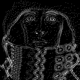
(c) Mask L1-ADJ-H.

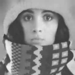
(d) Reconstruction with L1-ADJ-H.

(e) Mask H1-T.

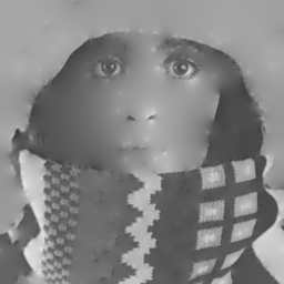
(f) Reconstruction with H1-T.

(g) Mask H1-H.

(h) Reconstruction with H1-H.

Figure 3: Masks and reconstructions from image without noise and with $10\%$ of total pixels saved.

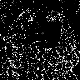
(a) Mask L1-ADJ-T.

(b) Reconstruction with L1-ADJ-T.

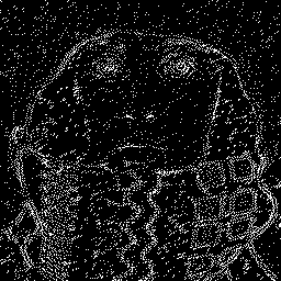
(c) Mask L1-ADJ-H.

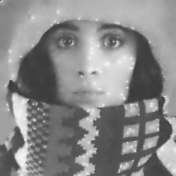
(d) Reconstruction with L1-ADJ-H.

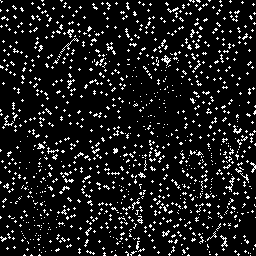
(e) Mask H1-T.

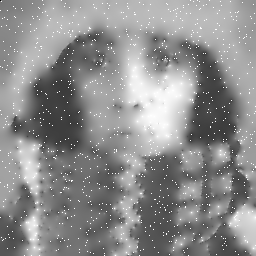
(f) Reconstruction with H1-T.

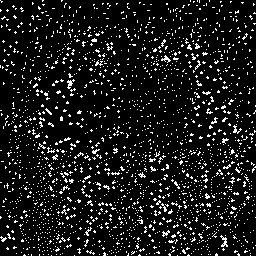
(g) Mask H1-H.

(h) Reconstruction with H1-H.

Figure 4: Masks and reconstructions from image with $2\%$ of salt noise and with $10\%$ of total pixels saved.

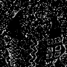
(a) Mask L1-ADJ-T.

(b) Reconstruction with L1-ADJ-T.

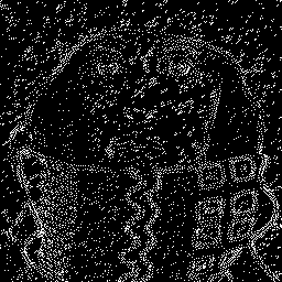
(c) Mask L1-ADJ-H.

(d) Reconstruction with L1-ADJ-H.

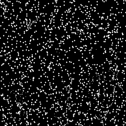
(e) Mask H1-T.

(f) Reconstruction with H1-T.

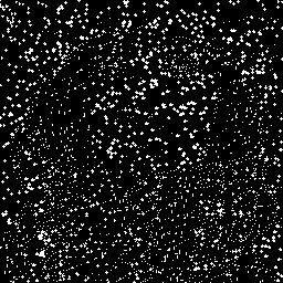
(g) Mask H1-H.

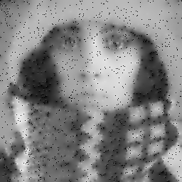
(h) Reconstruction with H1-H.

Figure 5: Masks and reconstructions from image with $2\%$ of pepper noise and with $10\%$ of total pixels saved.

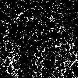
(a) Mask L1-ADJ-T.

(b) Reconstruction with L1-ADJ-T.

(c) Mask L1-ADJ-H.

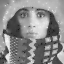
(d) Reconstruction with L1-ADJ-H.

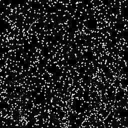
(e) Mask H1-T.

(f) Reconstruction with H1-T.

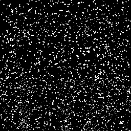
(g) Mask H1-H.

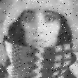
(h) Reconstruction with H1-H.

Figure 6: Masks and reconstructions from image with $2\%$ of salt and pepper noise and with $10\%$ of total pixels saved.

4.2 Gaussian Noise

Now, we consider images with gaussian noise. In this case we take $p=2$, and although the algorithms which are not based on the adjoint method perform well, we notice that this method gives better results again. We give in Table 4, Table 5 and Table 6 the $L^{2}$-error for the methods L2-ADJ-T, L2-ADJ-H, H1-T and H1-H with respect to the deviation $\sigma>0$ of gaussian noise. Formally, the criterion $-\widetilde{v}_{0}\,\widetilde{w}_{0}$ is close to $|\Delta f|^{2}$ which is similar to the result found in [7], but the fact that the adjoint state $w$ and primal variable $v$ are computed by solving linear PDEs improves distribution of the topological derivative. We see that for a reasonable level of noise, the L2-ADJ-H gives lower $L^{2}$-error and that the reconstructed image seems to have less noise than the original one. Similarly to L1-ADJ-methods, we can distinguish the edges of the image in the L2-ADJ-masks, while its not the case with the H1-methods.

We plot in Figure 8, Figure 9 and Figure 10 the resulting masks and reconstruction from various noise level.

Noise	L2-ADJ-T		L2-ADJ-H		H1-T	H1-H
$\sigma$	$\alpha$	$\|f-u\|_{2}$	$\alpha$	$\|f-u\|_{2}$	$\|f-u\|_{2}$	$\|f-u\|_{2}$
0	0.01	35.02	2.62	16.98	34.46	11.43
0.03	0.31	13.94	1.37	9.62	16.02	13.95
0.05	0.66	15.88	2.07	12.56	19.85	16.64
0.1	1.16	28.58	1.81	23.40	30.35	24.24
0.2	0.01	67.07	0.01	52.58	66.36	41.54

Table 4: $L^{2}$-error between the original image $f$ and the reconstruction $u$ (build from $f_{\delta}$) with $5\%$ of total pixels saved.

Noise	L2-ADJ-T		L2-ADJ-H		H1-T	H1-H
$\sigma$	$\alpha$	$\|f-u\|_{2}$	$\alpha$	$\|f-u\|_{2}$	$\|f-u\|_{2}$	$\|f-u\|_{2}$
0	0.01	23.08	0.01	9.70	22.99	6.02
0.03	0.71	8.88	0.96	7.76	11.49	10.38
0.05	0.86	13.42	0.76	12.50	15.74	13.85
0.1	0.71	26.81	0.66	24.40	27.01	23.42
0.2	0.01	55.74	2.27	47.17	55.32	42.12

Table 5: $L^{2}$-error between the original image $f$ and the reconstruction $u$ (build from $f_{\delta}$) with $10\%$ of total pixels saved.

Noise	L2-ADJ-T		L2-ADJ-H		H1-T	H1-H
$\sigma$	$\alpha$	$\|f-u\|_{2}$	$\alpha$	$\|f-u\|_{2}$	$\|f-u\|_{2}$	$\|f-u\|_{2}$
0	0.01	11.62	0.01	6.58	11.26	3.96
0.03	0.71	7.98	0.56	7.64	9.78	8.92
0.05	0.51	12.81	0.66	12.28	14.18	12.92
0.1	0.31	25.79	0.76	24.62	25.59	23.50
0.2	0.01	50.94	1.11	47.25	50.59	42.90

Table 6: $L^{2}$-error between the original image $f$ and the reconstruction $u$ (build from $f_{\delta}$) with $15\%$ of total pixels saved.

(a) Without noise.

(b) $\sigma=0.03$.

(c) $\sigma=0.05$.

(d) $\sigma=0.1$.

Figure 7: Input images $f_{\delta}$ with gaussian noise of deviation $\sigma$.

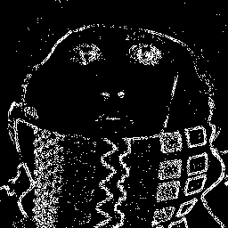
(a) Mask L2-ADJ-T.

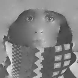
(b) Reconstruction with L2-ADJ-T.

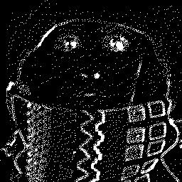
(c) Mask L2-ADJ-H.

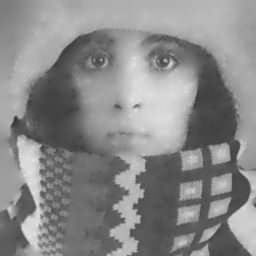
(d) Reconstruction with L2-ADJ-H.

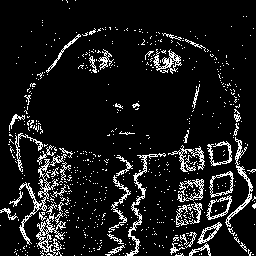
(e) Mask H1-T.

(f) Reconstruction with H1-T.

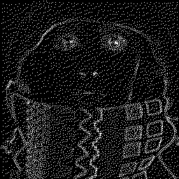
(g) Mask H1-H.

(h) Reconstruction with H1-H.

Figure 8: Masks and reconstructions from image without noise and with $10\%$ of total pixels saved.

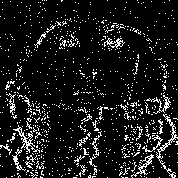
(a) Mask L2-ADJ-T.

(b) Reconstruction with L2-ADJ-T.

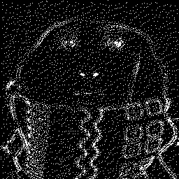
(c) Mask L2-ADJ-H.

(d) Reconstruction with L2-ADJ-H.

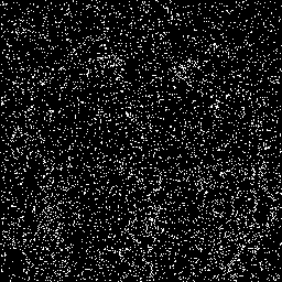
(e) Mask H1-T.

(f) Reconstruction with H1-T.

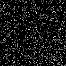
(g) Mask H1-H.

(h) Reconstruction with H1-H.

Figure 9: Masks and reconstructions from image with gaussian noise of deviation $\sigma=0.03$ and with $10\%$ of total pixels saved.

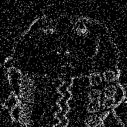
(a) Mask L2-ADJ-T.

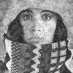
(b) Reconstruction with L2-ADJ-T.

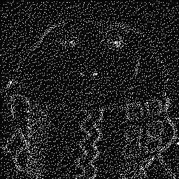
(c) Mask L2-ADJ-H.

(d) Reconstruction with L2-ADJ-H.

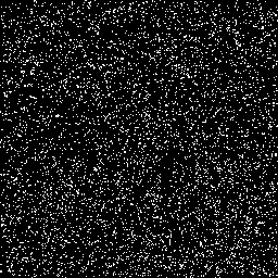
(e) Mask H1-T.

(f) Reconstruction with H1-T.

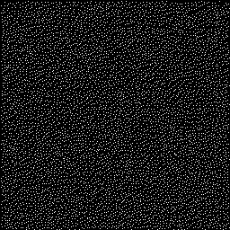
(g) Mask H1-H.

(h) Reconstruction with H1-H.

Figure 10: Masks and reconstructions from image with gaussian noise of deviation $\sigma=0.1$ and with $10\%$ of total pixels saved.

Conclusion and Discussions

In this article, we have formulated the PDE-based compression problem as a shape optimization one, and we have performed the topological expansion for the optimality condition by the adjoint method. Following the approaches of [2] and [14], we compute the asymptotic development for variations of the cost functionals with general exponents $p\geq 1$, which leads to an analytic soft threshold criterion to select relevant pixels of the mask. The inpainting from the masks to reconstruct the images is performed with a Laplacian, but all the approach may be extended without significant changes to more involved linear operator of second order. Moreover, it can be extended to other (linear and non linear) elliptic operators, and other form of insertions (not necessarily discs) at the price of some technicalities and computations details. Finally, we presented some numerical experiments in the case of the $L^{2}$-error and of a regularized $L^{1}$-error. It appears that this method for selecting the mask outperform the other expansions when the image to compress contains gaussian noise or impulse noise and is easy to implement with a reasonable cost, the adjoint problem is linear even if the operator for the reconstruction is nonlinear.

Appendix A Preliminaries

A.1 Recall on the Sobolev Norms

We recall the definition of the norms and some of their properties used in the proofs. Let $\mathcal{O}$ be an open subset of $\mathbb{R}^{2}$. For $v$ in $H^{1}(\mathcal{O})$, we recall the following Sobolev norms :

$$\begin{array}[]{ll}\|v\|_{0,\mathcal{O}}:=\left(\int_{\mathcal{O}}v^{2}\ dx\right)^{1/2},&|v|_{1,\mathcal{O}}:=\left(\int_{\mathcal{O}}|\nabla v|^{2}\ dx\right)^{1/2},\\ \|v\|_{1,\mathcal{O}}:=\left(\int_{\mathcal{O}}v^{2}\ dx+\int_{\mathcal{O}}|\nabla v|^{2}\ dx\right)^{1/2},&\|v\|_{1,\alpha,\mathcal{O}}:=\left(\int_{\mathcal{O}}v^{2}\ dx+\alpha\int_{\mathcal{O}}|\nabla v|^{2}\ dx\right)^{1/2}.\end{array}$$

Now we set $\mathcal{O}_{\varepsilon}:=\{x/\varepsilon\ |\ x\in\mathcal{O}\}$. Straightforward computations give :

Proposition A.1.

$$\|u(\cdot/\varepsilon)\|_{0,\mathcal{O}}=\varepsilon\|u\|_{0,\mathcal{O}_{\varepsilon}},$$

$$|u(\cdot/\varepsilon)|_{1,\mathcal{O}}=|u|_{1,\mathcal{O}_{\varepsilon}}.$$

On the boundary of a ball of radius $r>0$, namely $\partial B_{r}$, we define for $\phi$ in $H^{1/2}(\partial B_{r})$,

$$\|\phi\|_{1/2,\partial B_{r}}:=\inf_{u=\phi\ \text{on}\ \Gamma}\|u\|_{1,B_{r}\setminus B_{r/2}},$$

and for $\psi$ in $H^{-1/2}(\partial B_{r})$, we define the dual norm,

$$\|\psi\|_{-1/2,\partial B_{r}}:=\sup_{v\in H^{1/2}(\partial B_{r}),\,\|v\|_{1/2,\partial B_{r}}=1}\int_{\partial B_{r}}\psi\,v\ d\sigma.$$

Then, it is standard that

Proposition A.2.

Let $\psi\in H^{1}(B_{R}\setminus B_{R/2})$, with $-\alpha\Delta\psi+\psi=0$ in $B_{R}\setminus B_{R/2}$, there exists $C>0$, such that

$$\|\nabla\psi\cdot n\|_{-1/2,\partial B_{R}}\leq C\,\|\psi\|_{1,B_{R}\setminus B_{R/2}}.$$

A.2 Exterior Problem

Now, we give estimates of the solution to the exterior problem with the norms defined previously. For $\phi$ in $H^{1/2}(\partial B_{1})$, we define the exterior problem as the following :

$$\left\{\begin{array}[]{cl}-\alpha\Delta v_{\omega}+v_{\omega}=0,&\text{in}\ \mathbb{R}^{2}\setminus B_{1},\\ v_{\omega}=\phi,&\text{on}\ \partial B_{1},\\ v_{\omega}=0,&\text{at}\ \infty.\end{array}\right.$$

The aim of this appendix is to prove the following proposition :

Proposition A.3.

There exists $C_{1},C_{2},C_{3},C_{4},C_{5}$ and $C_{6}$ only dependant on $\alpha$ such that, for $\varepsilon$ small enough,

$$\|v_{\omega}\|_{0,B_{R/\varepsilon}\setminus B_{1}} \leq C_{1}\,\|\phi\|_{1/2,\partial B_{1}},$$

$$|v_{\omega}|_{1,B_{R/\varepsilon}\setminus B_{1}} \leq C_{2}\,\|\phi\|_{1/2,\partial B_{1}},$$

$$\|v_{\omega}\|_{1,B_{R/\varepsilon}\setminus B_{1}} \leq C_{3}\,\|\phi\|_{1/2,\partial B_{1}},$$

$$\|v_{\omega}\|_{0,B_{R/\varepsilon}\setminus B_{R/(2\varepsilon)}} \leq C_{4}\,e^{-R/(2\varepsilon\sqrt{\alpha})}\,\|\phi\|_{1/2,\partial B_{1}},$$

$$|v_{\omega}|_{1,B_{R/\varepsilon}\setminus B_{R/(2\varepsilon)}} \leq C_{5}\,e^{-R/(2\varepsilon\sqrt{\alpha})}\,\|\phi\|_{1/2,\partial B_{1}},$$

$$\|v_{\omega}\|_{1,B_{R/\varepsilon}\setminus B_{R/(2\varepsilon)}} \leq C_{6}\,e^{-R/(2\varepsilon\sqrt{\alpha})}\,\|\phi\|_{1/2,\partial B_{1}}.$$

The proposition above can be derived easily from the results bellow :

Proposition A.4.

For $y$ in $\mathbb{R}^{2}\setminus\overline{B_{1}}$, we have

$$v_{\omega}(y)=\int_{\partial B_{1}}E(y-x)p(x)\ d\sigma(x),$$

where $E$ is the fundamental solution (radial) in $\mathbb{R}^{2}\setminus\{0\}$ given by

$$E(y):=\frac{1}{2\pi}K_{0}\left(\frac{1}{\sqrt{\alpha}}|y|\right),$$

where $K_{0}$ is the modified Bessel function of the second kind [22] and $p$ is the solution in $H^{-1/2}(\partial B_{1})$ of

$$\int_{\partial B_{1}}E(y-x)p(x)\ d\sigma(x)=\phi(y),\ \forall y\in\partial B_{1}.$$

Proof.

We differentiate and we use [22] : $K_{0}^{\prime}(z)=-K_{1}(z)$ and $K_{1}^{\prime}(z)=-K_{0}(z)-\frac{1}{z}K_{1}(z)$. ∎

Proposition A.5.

For $|y|$ large enough, it exists $C_{1}$ and $C_{2}$, only dependant on $\alpha$, such that,

$$|v_{\omega}(y)| \leq C_{1}\,|y|^{-1/2}e^{-|y|/\sqrt{\alpha}}\,\|\phi\|_{1/2,\partial B_{1}},$$

$$|\nabla v_{\omega}(y)| \leq C_{2}\,|y|^{-1/2}e^{-|y|/\sqrt{\alpha}}\,\|\phi\|_{1/2,\partial B_{1}}.$$

Proof.

Since $K_{0}$ is a positive and decreasing function, we have for $(x,z)\in(\partial B_{1})^{2}$,

$$E(x-z)\geq\frac{1}{2\pi}K_{0}(2\alpha^{-1/2})\Leftrightarrow\frac{2\pi}{K_{0}(2\alpha^{-1/2})}E(x-z)\geq 1.$$

Then, for $z\in\partial B_{1}$,

$$\left|\int_{\partial B_{1}}p(x)d\sigma(x)\right|\leq\frac{2\pi}{K_{0}(2\alpha^{-1/2})}\left|\int_{\partial B_{1}}E(x-z)p(x)\ d\sigma(x)\right|=\frac{2\pi}{K_{0}(2\alpha^{-1/2})}|\phi(z)|.$$

We integrate on $\partial B_{1}$ with respect to $z$ the square of the previous inequality and get,

$$\left|\int_{\partial B_{1}}p(x)d\sigma(x)\right|^{2}\leq\frac{2\pi}{K_{0}(2\alpha^{-1/2})^{2}}\int_{\partial B_{1}}|\phi(z)|^{2}\ d\sigma(z).$$

Let $u=\phi$ on $\partial B_{1}$. Then,

$$\left|\int_{\partial B_{1}}p(x)d\sigma(x)\right|^{2}\leq\frac{2\pi}{K_{0}(2\alpha^{-1/2})^{2}}\int_{B_{1}\setminus B_{1/2}}|u(z)|^{2}\ dz,$$

this been true for every $u$, we take the $\sup$,

$$\left|\int_{\partial B_{1}}p(x)d\sigma(x)\right|^{2}\leq\frac{2\pi}{K_{0}(2\alpha^{-1/2})^{2}}\|\phi\|_{1/2,\partial B_{1}}^{2}.$$

With [22], we have for $z$ big enough,

$$K_{0}(z)=O(z^{-1/2}e^{-z}),$$

thus, there exists $C>0$, such that, for $|y|$ large enough,

$$|E(x-y)|\leq C\,|x-y|^{-1/2}e^{-|x-y|/\sqrt{\alpha}}.$$

Moreover, for $|y|$ large enough,

$$|x-y|^{-1/2}e^{-|x-y|/\sqrt{\alpha}}\leq C|y|^{-1/2}e^{-|y|/\sqrt{\alpha}},$$

then,

$$|E(x-y)|\leq C^{\prime}\,|y|^{-1/2}e^{-|y|/\sqrt{\alpha}}.$$

Therefore

$$|v_{\omega}(y)|\leq C_{1}\,|y|^{-1/2}e^{-|y|/\sqrt{\alpha}}\,\|\phi\|_{1/2,\partial B_{1}}.$$

Next,

$$\partial_{y_{i}}v_{\omega}(y)=\partial_{y_{i}}\int_{\partial B_{1}}E(y-x)p(x)\ d\sigma(x)=\int_{\partial B_{1}}\partial_{y_{i}}E(y-x)p(x)\ d\sigma(x),$$

and

$$\partial_{y_{i}}E(x-y)=\frac{1}{2\pi}\partial_{y_{i}}K_{0}(\alpha^{-1/2}|x-y|)=\frac{-1}{2\pi}\alpha^{-1/2}\,|y-x|^{-1}K_{1}(\alpha^{-1/2}|y-x|)\,y_{i}.$$

Thus

$$|\nabla v_{\omega}(y)|=\frac{1}{2\pi}\alpha^{-1/2}\,|y|\,\left|\int_{\partial B_{1}}|y-x|^{-1}K_{1}(\alpha^{-1/2}|y-x|)\,p(x)\ d\sigma(x)\right|,$$

in the same way that before, for $|y|$ big enough, [22],

$$|\nabla v_{\omega}(y)|\leq C\,|y|^{-1/2}e^{-|y|/\sqrt{\alpha}}\,\|\phi\|_{1/2,\partial B_{1}}.$$

∎

A.3 Some Estimates for the Various Elliptic Problems in the Previous Sections

In this appendix, we give the estimates of the solution of the problem below with the norms defined in Appendix A.1.

Proposition A.6.

Let $\psi\in H^{1/2}(\partial B_{\varepsilon})$ and $\phi\in H^{1/2}(\partial B_{R})$. Let $v_{\varepsilon}$ be the solution of the problem below :

$$\left\{\begin{array}[]{cl}-\alpha\Delta v_{\varepsilon}+v_{\varepsilon}=0,&\text{in}\ B_{R}\setminus B_{\varepsilon},\\ v_{\varepsilon}=\psi,&\text{on}\ \partial B_{\varepsilon},\\ v_{\varepsilon}=\phi,&\text{on}\ \partial B_{R}.\end{array}\right.$$

Then, for $\varepsilon$ small enough,

$$\|v_{\varepsilon}\|_{0,B_{R}\setminus B_{\varepsilon}} \leq C_{1}\,\big{(}\|\phi\|_{1/2,\partial B_{R}}+e^{-R/(2\varepsilon\sqrt{\alpha})}\,\|\psi(\varepsilon\,\cdot)\|_{1/2,\partial B_{1}}\big{)},$$

$$|v_{\varepsilon}|_{1,B_{R}\setminus B_{\varepsilon}} \leq C_{2}\,\big{(}\|\phi\|_{1/2,\partial B_{R}}+e^{-R/(2\varepsilon\sqrt{\alpha})}\,\|\psi(\varepsilon\,\cdot)\|_{1/2,\partial B_{1}}\big{)},$$

$$\|v_{\varepsilon}\|_{0,B_{R}\setminus B_{R/2}} \leq C_{3}\,\big{(}\|\phi\|_{1/2,\partial B_{R}}+e^{-R/(2\varepsilon\sqrt{\alpha})}\,\|\psi(\varepsilon\,\cdot)\|_{1/2,\partial B_{1}}\big{)},$$

$$|v_{\varepsilon}|_{1,B_{R}\setminus B_{R/2}} \leq C_{4}\,\big{(}\|\phi\|_{1/2,\partial B_{R}}+e^{-R/(2\varepsilon\sqrt{\alpha})}\,\|\psi(\varepsilon\,\cdot)\|_{1/2,\partial B_{1}}\big{)}.$$

The proposition above can be derived easily from the results bellow :

Lemma A.1.

Let $\phi\in H^{1/2}(\partial B_{R})$. Let $v_{\varepsilon}$ be the solution of the following problem :

$$\left\{\begin{array}[]{cl}-\alpha\Delta v_{\varepsilon}+v_{\varepsilon}=0,&\text{in}\ B_{R}\setminus B_{\varepsilon},\\ v_{\varepsilon}=0,&\text{on}\ \partial B_{\varepsilon},\\ v_{\varepsilon}=\phi,&\text{on}\ \partial B_{R}.\end{array}\right.$$

Then, it exists $0<\varepsilon_{0}<R$ and $C>0$ such that, for all $0<\varepsilon<\varepsilon_{0}$, we have

$$\|v_{\varepsilon}\|_{1,B_{R}\setminus B_{\varepsilon}}\leq C\|\phi\|_{1/2,\partial B_{R}}.$$

Proof.

Let $R/2<\varepsilon_{0}<R$, them it is readily checked that :

$$\|v_{\varepsilon_{0}}\|_{1,\alpha,B_{R}\setminus B_{\varepsilon_{0}}}\leq C\|v\|_{1,B_{R}\setminus B_{R/2}}.$$

Next, we take $\varepsilon<\varepsilon_{0}$. Then, $D_{\varepsilon_{0}}\subset D_{\varepsilon}$ and we denote by $\widetilde{v}_{\varepsilon_{0}}$ the extension by $0$ of $v_{\varepsilon_{0}}$ to $D_{\varepsilon}$. As $v_{\varepsilon}$ is solution of the problem, it follows :

$$\|v_{\varepsilon}\|_{1,B_{R}\setminus B_{\varepsilon}}\leq C\|v_{\varepsilon}\|_{1,\alpha,B_{R}\setminus B_{\varepsilon}}.$$

∎

Lemma A.2.

Let $\psi\in H^{1/2}(\partial B_{\varepsilon})$. Let $v_{\varepsilon}$ be the solution of the following problem :

$$\left\{\begin{array}[]{cl}-\alpha\Delta v_{\varepsilon}+v_{\varepsilon}=0,&\text{in}\ B_{R}\setminus B_{\varepsilon},\\ v_{\varepsilon}=\psi,&\text{on}\ \partial B_{\varepsilon},\\ v_{\varepsilon}=0,&\text{on}\ \partial B_{R}.\end{array}\right.$$

Then, for $\varepsilon$ small enough,

$$\|v_{\varepsilon}\|_{0,B_{R}\setminus B_{\varepsilon}} \leq C_{1}\,e^{-R/(2\varepsilon\sqrt{\alpha})}\,\|\psi(\varepsilon\,\cdot)\|_{1/2,\partial B_{1}},$$

$$|v_{\varepsilon}|_{1,B_{R}\setminus B_{\varepsilon}} \leq C_{2}\,e^{-R/(2\varepsilon\sqrt{\alpha})}\,\|\psi(\varepsilon\,\cdot)\|_{1/2,\partial B_{1}},$$

$$\|v_{\varepsilon}\|_{0,B_{R}\setminus B_{R/2}} \leq C_{3}\,e^{-R/(2\varepsilon\sqrt{\alpha})}\,\|\psi(\varepsilon\,\cdot)\|_{1/2,\partial B_{1}}$$

$$|v_{\varepsilon}|_{1,B_{R}\setminus B_{R/2}} \leq C_{4}\,e^{-R/(2\varepsilon\sqrt{\alpha})}\,\|\psi(\varepsilon\,\cdot)\|_{1/2,\partial B_{1}}.$$

Proof.

We consider the following exterior problem :

$$\left\{\begin{array}[]{cl}-\alpha\Delta v_{\omega_{\varepsilon}}+v_{\omega_{\varepsilon}}=0,&\text{in}\ \mathbb{R}^{2}\setminus B_{1},\\ v_{\omega_{\varepsilon}}=\psi(\varepsilon\,\cdot),&\text{on}\ \partial B_{1},\\ v_{\omega_{\varepsilon}}=0,&\text{at}\ \infty.\end{array}\right.$$

Therefore,

$$v_{\varepsilon}=v_{\omega_{\varepsilon}}(\cdot/\varepsilon)|_{B_{R}\setminus B_{\varepsilon}}-w_{\varepsilon},$$

where $w_{\varepsilon}$ is solution of

$$\left\{\begin{array}[]{cl}-\alpha\Delta w_{\varepsilon}+w_{\varepsilon}=0,&\text{in}\ B_{R}\setminus B_{\varepsilon},\\ w_{\varepsilon}=0,&\text{on}\ \partial B_{\varepsilon},\\ w_{\varepsilon}=v_{\omega_{\varepsilon}}(\cdot/\varepsilon),&\text{on}\ \partial B_{R}.\end{array}\right.$$

Using Proposition A.1 and Proposition A.3, for $\varepsilon$ small enough, we have

$$\|w_{\varepsilon}\|_{1,B_{R}\setminus B_{\varepsilon}} \leq C\,e^{-R/(2\varepsilon\sqrt{\alpha})}\,\|\psi(\varepsilon\,\cdot)\|_{1/2,\partial B_{1}}.$$

It follows from scaling argument,

$$\|v_{\varepsilon}\|_{0,B_{R}\setminus B_{\varepsilon}} \leq\|v_{\omega_{\varepsilon}}(\cdot/\varepsilon)\|_{0,B_{R}\setminus B_{\varepsilon}}+\|w_{\varepsilon}\|_{0,B_{R}\setminus B_{\varepsilon}}$$

$$\leq C\,e^{-R/(2\varepsilon\sqrt{\alpha})}\,\|\psi(\varepsilon\,\cdot)\|_{1/2,\partial B_{1}}.$$

The other estimations are obtained similarly. ∎

References

- [1] R. D. Adam, P. Peter, and J. Weickert, Denoising by Inpainting, in Scale Space and Variational Methods in Computer Vision, F. Lauze, Y. Dong, and A. B. Dahl, eds., Lecture Notes in Computer Science, Cham, 2017, Springer International Publishing, pp. 121–132.
- [2] S. Amstutz, Sensitivity analysis with respect to a local perturbation of the material property, Asymptotic Analysis, 49 (2006).
- [3] S. Andris, P. Peter, and J. Weickert, A proof-of-concept framework for PDE-based video compression, in 2016 Picture Coding Symposium (PCS), Dec. 2016, pp. 1–5. ISSN: 2472-7822.
- [4] E. Bae and J. Weickert, Partial Differential Equations for Interpolation and Compression of Surfaces, in Mathematical Methods for Curves and Surfaces, M. Dæhlen, M. Floater, T. Lyche, J.-L. Merrien, K. Mørken, and L. L. Schumaker, eds., Lecture Notes in Computer Science, Berlin, Heidelberg, 2010, Springer, pp. 1–14.
- [5] Z. Belhachmi, A. Ben Abda, B. Meftahi, and H. Meftahi, Topology optimization method with respect to the insertion of small coated inclusion, Asymptot. Anal., (2018).
- [6] Z. Belhachmi, D. Bucur, B. Burgeth, and J. Weickert, How to Choose Interpolation Data in Images, SIAM Journal of Applied Mathematics, 70 (2009), pp. 333–352.
- [7] Z. Belhachmi and T. Jacumin, Optimal interpolation data for PDE-based compression of images with noise, Communications in Nonlinear Science and Numerical Simulation, 109 (2022), p. 106278.
- [8] M. Bertalmio, G. Sapiro, V. Caselles, and C. Ballester, Image inpainting, in Proceedings of the 27th annual conference on Computer graphics and interactive techniques, SIGGRAPH ’00, USA, July 2000, ACM Press/Addison-Wesley Publishing Co., pp. 417–424.
- [9] F. Catté, P.-L. Lions, J.-M. Morel, and T. Coll, Image Selective Smoothing and Edge Detection by Nonlinear Diffusion, SIAM Journal on Numerical Analysis, 29 (1992), pp. 182–193. Publisher: Society for Industrial and Applied Mathematics.
- [10] J. Cea, A. Gioan, and J. Michel, Quelques resultats sur l’identification de domaines, CALCOLO, 10 (1973), pp. 207–232.
- [11] T. Chan and J. Shen, Nontexture Inpainting by Curvature-Driven Diffusions, Journal of Visual Communication and Image Representation, 12 (2001), pp. 436–449.
- [12] R. W. Floyd and L. Steinberg, Adaptive algorithm for spatial greyscale, Proceedings of the Society for Information Display, 17 (1976), pp. 75–77.
- [13] I. Galić, J. Weickert, M. Welk, A. Bruhn, A. Belyaev, and H.-P. Seidel, Image Compression with Anisotropic Diffusion, Journal of Mathematical Imaging and Vision, 31 (2008), pp. 255–269.
- [14] S. Garreau, P. Guillaume, and M. Masmoudi, The Topological Asymptotic for PDE Systems: The Elasticity Case, SIAM J. Control and Optimization, 39 (2001), pp. 1756–1778.
- [15] P. Guillaume and K. Idris, The Topological Asymptotic Expansion for the Dirichlet Problem, SIAM J. Control and Optimization, 41 (2002), pp. 1042–1072.
- [16] S. Larnier, J. Fehrenbach, and M. Masmoudi, The Topological Gradient Method: From Optimal Design to Image Processing, Milan Journal of Mathematics, 80 (2012).
- [17] F. Lenzen and O. Scherzer, Partial Differential Equations for Zooming, Deinterlacing and Dejittering, International Journal of Computer Vision, 92 (2011), pp. 162–176.
- [18] S. Masnou and J.-M. Morel, Level lines based disocclusion, in Proceedings 1998 International Conference on Image Processing. ICIP98 (Cat. No.98CB36269), Oct. 1998, pp. 259–263 vol.3.
- [19] R. M. K. Mohideen, P. Peter, T. Alt, J. Weickert, and A. Scheer, Compressing Colour Images with Joint Inpainting and Prediction, arXiv:2010.09866 [eess], (2020). arXiv: 2010.09866.
- [20] M. Nikolova, Minimizers of Cost-Functions Involving Nonsmooth Data-Fidelity Terms. Application to the Processing of Outliers, SIAM J. Numerical Analysis, 40 (2002), pp. 965–994.
- [21] , A Variational Approach to Remove Outliers and Impulse Noise, Journal of Mathematical Imaging and Vision, 20 (2004).
- [22] K. Oldham, J. Myland, and J. Spanier, An Atlas of Functions, Springer US, 2009. Publication Title: An Atlas of Functions.
- [23] P. Perona and J. Malik, Scale-space and edge detection using anisotropic diffusion, IEEE Transactions on Pattern Analysis and Machine Intelligence, 12 (1990), pp. 629–639. Conference Name: IEEE Transactions on Pattern Analysis and Machine Intelligence.
- [24] P. Peter and J. Weickert, Colour image compression with anisotropic diffusion, 2014 IEEE International Conference on Image Processing, ICIP 2014, (2015), pp. 4822–4826.
- [25] O. Scherzer, M. Grasmair, H. Grossauer, M. Haltmeier, and F. Lenzen, Variational Methods in Imaging, Springer Science & Business Media, Sept. 2008. Google-Books-ID: 6tq9DiTVnfAC.
- [26] C. Schmaltz, J. Weickert, and A. Bruhn, Beating the Quality of JPEG 2000 with Anisotropic Diffusion, in Pattern Recognition, J. Denzler, G. Notni, and H. Süße, eds., Lecture Notes in Computer Science, Berlin, Heidelberg, 2009, Springer, pp. 452–461.
- [27] R. Ulichney, Digital Halftoning, MIT Press, Cambridge, MA, USA, June 1987.
- [28] J. Weickert, Theoretical Foundations Of Anisotropic Diffusion In Image Processing, Computing, Suppl, 11 (1996), pp. 221–236.
- [29] J. Weickert, S. Ishikawa, and A. Imiya, Linear Scale-Space has First been Proposed in Japan, Journal of Mathematical Imaging and Vision, 10 (1999), pp. 237–252.
- [30] W. P. Ziemer, Extremal length and $p$-capacity., Michigan Mathematical Journal, 16 (1969), pp. 43–51. Publisher: University of Michigan, Department of Mathematics.