Statistical reconstruction of pulse shapes
from pulse streams

Abstract

A short sample sequence of a finite-length pulse signal allows for its reconstruction only if the signal has a sparse representation in some basis. The recurrence of the pulse allows for a statistical approach to its reconstruction. We propose a novel method for this task. It is based on the distribution of short sample sequences treated as points that lie along a closed curve in a low-dimensional Euclidean space. We prove that the probability distribution of the points along this curve determines the underlying pulse signal uniquely. Based on this discovery, we propose an algorithm for pulse estimation from a finite number of short sequences of pulse-stream samples.

I Introduction

Signals comprised of a stream of short pulses, referred to as pulse streams, appear in many applications, including biomedicine [1], radar [2], and ultrasonics [3, 4]. In general, Shannon sampling theorem requires a high sampling rate for the good-quality reconstruction of short pulses. If the pulses have a sparse representation in some basis, then it is possible to reconstruct them from samples taken at a much lower sub-Nyquist frequency by the compressed sampling technique [3, 5, 6]. Sub-Nyquist sampling is also possible if the pulse shapes are known up to their amplitudes and inter-pulse distances [7, 8]. In our study, we do not assume prior knowledge of the pulse shape nor restrict the pulse to have a sparse representation. Instead, we assume that the pulse stream consists of a pulse that recurs in time, and we set the reconstruction of the shape of this single pulse as our goal. The main contribution of this paper is as follows:

• It shows that a single pulse can be reconstructed from the probability distribution of short sample sequences taken at a sub-Nyquist rate.

• It shows how to estimate the pulse from a finite number of these sequences.

We propose reconstruction algorithms based on the study of the probability distribution of short sample sequences, referred to as sample trains. Such an approach was introduced in our papers [9, 10, 11, 12] in the context of periodic signals.

The paper is organized as follows. The next section shows the relationship between sample trains, pulse signals, and pulse streams. Sections III and IV are devoted to the algorithms for pulse reconstruction from the probability distribution of sample trains and a finite number of sample trains, respectively. Section V presents the results of numerical simulations of the latter algorithm. The paper is concluded in Section VI.

II Pulse signals and pulse streams

We define pulse signals as continuous-time signals with finite support. Without loss of generality, we assume that for any pulse signal $p$, the smallest interval outside of which the signal vanishes is of the form $(0,T_{p})$, where $T_{p}>0$ is the pulse length; see Fig. 2. A pulse stream is a signal that consists of copies of the same pulse signal, i.e., it is a signal of the following form, where $N$ may take a finite or $+\infty$ value.

$$s(t)=\sum_{i=1}^{N}p(t-t_{i}),\qquad t_{1}<t_{2}<\dots.$$ (1)

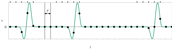
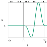
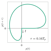
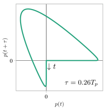
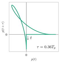
Figure 1: A pulse stream signal $s$ (to the left) and the underlying pulse signal $p$ (to the right). Small circles indicate the samples of the pulse stream. Ticks along the top edges of the plots show the corresponding starting times of non-zero sample trains of length $3$ and time-span $2\tau$.

Figure 2: The images of $\mathbf{p}_{2,\tau}$ for signal $p$ shown in Fig. 2, and three inter-sample distances $\tau=0.16T_{p}$, $\tau=0.26T_{p}$, $\tau=0.36T_{p}$

Fig. 2 shows an example of a pulse stream. The minimum distance between pulses that form signal $s$ is termed inter-pulse distance and is denoted by $\Delta_{s}$, i.e.,

$$\Delta_{s}=\min_{i=1,\dots,N}(t_{i+1}-t_{i}-T_{p}).$$ (2)

Sample trains of signal $p$ are defined as vectors of the form

$$\mathbf{p}_{d,\tau}(t)=[p(t),\,p(t+\tau),\,p(t+2\tau),\,\dots,\,p\left(t+d\tau\right)],$$ (3)

where $d\tau$ is the time span of the sample train, $t$ is its starting time, and $\tau$ is the inter-sample time distance. Note that sample trains $\mathbf{p}_{d,\tau}$ consist of $d+1$ samples. Therefore, $\mathbf{p}_{d,\tau}(t)$ can be treated as points in a $d+1$-dimensional Euclidean space. Assume that a pulse signal $p$ recurs in time, in a periodic or non-periodic manner, forming a pulse stream $s$. By sampling $s$ uniformly, one may acquire multiple sample trains of signal $p$ which correspond to various starting times $t_{0}\in\left(-d\tau,T_{p}\right)$; see Fig. 2. In particular, the sets of sample trains for the pulse stream and the underlying pulse signal coincide, provided that the following condition is satisfied.

Condition 1.

$\Delta_{s}\geq d\tau.$

III Distribution of sample trains

If $p$ is a pulse signal of length $T_{p}$, then $\mathbf{p}_{d,\tau}(t)$ is a train of zeros unless $-d\tau<t<T_{p}$. When $t$ varies in the range $(-d\tau,T_{p})$, then $\mathbf{p}_{d,\tau}(t)$ moves along a curve that lies in $\mathbf{R}^{d+1}$. Henceforth, this curve is denoted by $\mathcal{C}_{p,d,\tau}$. Three such curves are shown in Fig. 2.

A continuous mapping $\mathbf{q}\colon(0,a)\to\mathcal{C}_{p,d,\tau}$, $a>0$, will be called a regular parameterization of curve $\mathcal{C}_{p,d,\tau}$ if $\mathbf{q}$ is a one-to-one function onto $\mathcal{C}_{p,d,\tau}$. In this study, we focus on pulse signals $p$, inter-sample distances $\tau$, and sample-train lengths $d+1$ that satisfy the following condition.

Condition 2.

$\mathbf{p}_{d,\tau}$ restricted to interval $(-d\tau,T_{p})$ is a regular parameterization of curve $\mathcal{C}_{p,d,\tau}$.

The main obstacle to Condition 2 is the presence of self-intersections of curve $\mathcal{C}_{p,d,\tau}$. For example, signal from Fig. 2 satisfies Condition 2 for $d=2$ and $\tau=0.16T_{p}$ and it does not for $\tau=0.36T_{p}$ ($\mathcal{C}_{p,d,\tau}$ has self-intersections in the latter case as shown in the last graph of Fig. 2). If Condition 2 is satisfied, then there exist exactly two arc-length parameterizations of curve $\mathcal{C}=\mathcal{C}_{p,d,\tau}$. They have opposite orientations. The initial part of curve $\mathcal{C}_{p,d,\tau}$ can be tell from its terminal part by noting that the part that corresponds to $t<-d\tau+\tau$ lies in the $X_{d+1}$-axis, and the part that corresponds to $t>T_{p}-\tau$ lies in the $X_{1}$-axis; see Fig. 2. Let $\mathbf{r}_{\mathcal{C}}\colon(0,L)\to\mathbf{R}^{d+1}$ be the unique arc-length parameterization of $\mathcal{C}$ that maps initial segments of interval $(0,L)$ to initial segments of $\mathcal{C}$ ($L$ is the total length of $\mathcal{C}$). The probability distribution of starting times $t$ of sample trains $\mathbf{p}_{d,\tau}(t)$ results in the corresponding probability distribution of the trains treated as points of curve $\mathcal{C}_{p,d,\tau}$. By using parameterization $\mathbf{r}_{\mathcal{C}}$ we may pull-back this probability distribution from curve $\mathcal{C}$ to interval $(0,L)$. In particular, the uniform distribution of starting times $t\in(-d\tau,\,T_{p})$ determines a quantile function $Q_{p,d,\tau}\colon[0,1]\to[0,L]$. Quantile of order $\alpha$ of this distribution corresponds to starting time $t$ that lies in the $\alpha$ part of the distance from the left towards the right end of interval $(-d\tau,\,T_{p})$, i.e.,

$$\mathbf{r}_{\mathcal{C}}\left(Q_{p,d,\tau}(\alpha)\right)=\mathbf{p}_{d,\tau}\left(-d\tau+\alpha(T_{p}+d\tau)\right).$$ (4)

Let $\pi_{k}$ denote a function that picks the $k$-th coordinate of its argument, i.e., $\pi_{k}\left([x_{1},\dots,x_{m}]\right)=x_{k}$. The $k$-th coordinate of function $\mathbf{p}_{d,\tau}$, i.e., $\pi_{k}(\mathbf{p}_{d,\tau})$ vanishes outside the interval

$$I_{k}=\bigl{(}\left(1-k\right)\tau,\,T_{p}+\left(1-k\right)\tau\bigr{)}.$$ (5)

Let $\alpha_{k,\min}$ and $\alpha_{k,\max}$ denote the fractions of interval $(-d\tau,\,T_{p})$ that correspond to the ends of $I_{k}$, i.e.,

$$\alpha_{k,\min}=\frac{(d+1-k)\tau}{T_{p}+d\tau},\,\alpha_{k,\max}=\frac{T_{p}+(d+1-k)\tau}{T_{p}+d\tau}.$$ (6)

Consequently,

$$T_{p} =\frac{(d+1-k)\tau}{\alpha_{k,\min}}-d\tau, k =1,\dots,d,$$ (7)

$$T_{p} =\frac{(k-1)\tau}{1-\alpha_{k,\max}}-d\tau, k =2,\dots,d+1.$$ (8)

Let

$$\mathbf{q}(\alpha)=\begin{cases}\mathbf{r}_{\mathcal{C}}\left(Q_{p,d,\tau}(\alpha)\right)&\alpha\in(0,1)\\ 0&\alpha\geq 1.\end{cases}$$ (9)

By (4), $\mathbf{q}(\alpha)=\mathbf{p}_{d,\tau}\left(-d\tau+\alpha(T_{p}+d\tau)\right)$. Therefore, by (3)

$$p(t)=\pi_{k}\bigl{(}\mathbf{p}_{d,\tau}\left(t-(k-1)\tau\right)\bigr{)}\\ =\pi_{k}\left(\mathbf{q}\left(\frac{t+(d+1-k)\tau}{T_{p}+d\tau}\right)\right),k=1,\,\dots,\,d+1.$$ (10)

Eqs. (6)–(10) result in the following reconstruction algorithm.

Algorithm 1.

Inputs: Sample period $\tau$ and the probability distribution (supported on a curve $\mathcal{C}$) of sample trains $\mathbf{p}_{d,\tau}(t)$ that result from the uniform distribution of starting times $t$ for a pulse signal $p$ that satisfies Condition 2. Output: pulse signal $p$.

1. Take the arc-length parameterization $\mathbf{r}_{\mathcal{C}}\colon(0,L)\to\mathcal{C}$ that maps the initial segments of interval $(0,L)$ to the initial segments of $\mathcal{C}$.

2. Compute the quantile function $Q\colon[0,1]\to[0,L]$ of the $\mathbf{r}_{\mathcal{C}}$-pull-back of the given probability distribution.

3. Define mapping $\mathbf{q}$ according to (9) (by the assumption $Q_{p,d,\tau}=Q$) and find $T_{p}$ by any of Eqs. (7) or (8).

4. Compute signal $p$ by Eq. (10) for any $k=1,\dots,d+1$.

IV Pulse reconstruction from sample trains

The previous section shows how to reconstruct a pulse signal $p$ from the probability distribution supported on curve $\mathcal{C}=\mathcal{C}_{p,d,\tau}$. In practice, instead of such distribution and curve, we can have only a finite number of non-zero sample trains:

$$\mathbf{p}_{1},\,\mathbf{p}_{2},\,\dots,\,\mathbf{p}_{n}\in\mathbf{R}^{d+1}.$$ (11)

In this section, we show how to construct a reliable estimator of the pulse signal in such a practical scenario. We will approach the goal in three steps. First, we explain how to estimate curve $\mathcal{C}_{p,d,\tau}$. Then, we show how to estimate the probability distribution on this curve. Eventually, we will adjust Algorithm 1 to accomplish the goal.

IV-A Curve estimation

We can approximate curve $\mathcal{C}_{p,d,\tau}$ with a polygonal chain by connecting points (11) with line segments. To get a reasonable approximation, we need to find the order in which these points lie on curve $\mathcal{C}_{p,d,\tau}$. This can be accomplished, e.g., with the NN-CRUST algorithm [13] or its improved version presented in [14]. The NN-CRUST algorithm is proven to give the correct order of points along a curve, provided that the curve is sampled densely enough. However, it does not identify the endpoints of curve $\mathcal{C}_{p,d,\tau}$. Therefore, we complement the algorithm with the following postprocessing. Assume that the result of the NN-CRUST algorithm is an ordering of points (11) given by permutation $\eta$, i.e., $\mathbf{p}_{\eta_{1}},\,\dots,\,\mathbf{p}_{\eta_{n}}$. Let $\mathbf{p}_{\eta_{k}}$ be the point that lies on $x_{d+1}$-axis in the closest distance to the origin of the coordinate system. If $\mathbf{p}_{\eta_{k+1}}$ lies on $x_{d+1}$-axis as well, or if $\mathbf{p}_{\eta_{k-1}}$ lies on $x_{1}$-axis, then we replace permutation $\eta$ with $\eta^{\prime}$ defined as

$$\eta^{\prime}_{1}=\eta_{k},\,\eta^{\prime}_{2}=\eta_{k+1},\,\dots,\eta^{\prime}_{n}=\eta_{k+n-1},$$ (12)

where arithmetic operations on the indices are performed modulo $n$, e.g., $\eta_{n+1}=\eta_{1}$. In the opposite case, i.e., if neither $\mathbf{p}_{\eta_{k+1}}$ lies on $x_{d+1}$-axis nor $\mathbf{p}_{\eta_{k-1}}$ lies on $x_{1}$-axis, we set

$$\eta^{\prime}_{1}=\eta_{k},\,\eta^{\prime}_{2}=\eta_{k-1},\,\dots,\eta^{\prime}_{n}=\eta_{k-n+1}.$$ (13)

If NN-CRUST does not identify points (11) as belonging to a single closed curve or if no point of (11) lies on $x_{d}$-axis then we cannot determine the order in which points (11) lie on curve $\mathcal{C}$ and we have to stop the reconstruction procedure until more points are available.

IV-B Probability distribution estimation

Points $\mathbf{p}_{\eta^{\prime}_{1}},\,\dots,\,\mathbf{p}_{\eta^{\prime}_{n}}$ obtained in the previous subsection can be used as vertices of a polygonal chain that starts and ends at the origin. This chain approximates curve $\mathcal{C}_{p,d,\tau}$. Let $\hat{\mathbf{r}}_{\mathcal{C}}\colon(0,\hat{L})\to\mathbf{R}^{d+1}$ be the arc-length parameterization of this chain. In particular,

$$\hat{L}=\|\mathbf{p}_{\eta^{\prime}_{1}}-0\|+\sum_{k=1}^{n}\|\mathbf{p}_{\eta^{\prime}_{k+1}}-\mathbf{p}_{\eta^{\prime}_{k}}\|+\|0-\mathbf{p}_{\eta^{\prime}_{n}}\|.$$ (14)

We estimate the quantile function $Q_{p,d,\tau}$ introduced in Section III by first defining $\hat{Q}$ on a grid: $\hat{Q}\left(0\right)=0$, $\hat{Q}\left(1\right)=\hat{L}$, and

$$\hat{Q}\left(\frac{k-0.5}{n}\right)=\hat{\mathbf{r}}_{\mathcal{C}}^{-1}\left(\mathbf{p}_{\eta^{\prime}_{k}}\right),\,k=1,\,\dots,\,n.$$ (15)

Then, we linearly interpolate $\hat{Q}$ between the nodes of the grid. Eventually, we obtain an approximation $\hat{\mathbf{q}}$ of mapping $\mathbf{q}$ by Eq. (9), in which we replace, $Q_{p,d,\tau}$ and $\mathbf{r}_{\mathcal{C}}$ by $\hat{Q}$ and $\hat{\mathbf{r}}_{\mathcal{C}}$, respectively.

IV-C Pulse-reconstruction algorithm

Let $n_{k,\min}$ and $n_{k,\max}$ be the ordinal numbers of, respectively, the first and the last non-zero entries among

$$\pi_{k}\left(\mathbf{p}_{\eta^{\prime}_{1}}\right),\,\dots,\,\pi_{k}\left(\mathbf{p}_{\eta^{\prime}_{n}}\right).$$ (16)

We define the following estimators

$$\hat{\alpha}_{k,\min} =\frac{n_{k,\min}-1}{n}, k =1,\,\dots,\,d,$$ (17)

$$\hat{\alpha}_{k,\max} =\frac{n_{k,\max}}{n}, k =2,\,\dots,\,d+1.$$ (18)

and average Eqs. (7) and (8) to get a $T_{p}$ estimator:

$$\hat{T}_{p}=\frac{\tau}{2d}\left(\sum_{k=1}^{d}\frac{d+1-k}{\hat{\alpha}_{k,\min}}+\sum_{k=2}^{d+1}\frac{k-1}{1-\hat{\alpha}_{k,\max}}\right)-d\tau$$ (19)

Eventually, we estimate the pulse signal by averaging (10), i.e.,

$$\hat{p}(t)=\frac{1}{d+1}\sum_{k=1}^{d+1}\pi_{k}\left(\hat{\mathbf{q}}\left((t+(d+1-k)\tau)/(\hat{T}_{p}+d\tau)\right)\right).$$ (20)

The following algorithm concludes this section.

Algorithm 2.

Inputs: parameters $d$ and $\tau$, sample trains (11) of a pulse signal $p$ that satisfies Condition 2. Output: estimator $\hat{p}$ of pulse signal $p$

1. Order points (11) by the NN-CRUST algorithm.

2. Find permutation $\eta^{\prime}$ as explained in Subsection IV-A.

3. Compute the arc-length parameterization $\hat{\mathbf{r}}_{\mathcal{C}}$ of the polygonal chain with vertices $0,\,\mathbf{p}_{\eta^{\prime}_{1}},\,\dots,\,\mathbf{p}_{\eta^{\prime}_{n}},\,0$.

4. Compute quantile function $\hat{Q}$ by (15).

5. Compute function $\hat{\mathbf{q}}$ by (9) in which $\mathbf{q}$, $\mathbf{r}_{\mathcal{C}}$, and $Q_{p,d,\tau}$ are replaced with $\hat{\mathbf{q}}$, $\hat{\mathbf{r}}_{\mathcal{C}}$, and $\hat{Q}$, respectively.

6. Compute pulse length estimator $\hat{T}_{p}$ by (19).

7. Compute estimator $\hat{p}$ by (20).

Let us highlight that in Algorithm 2, the sample trains may also result from sampling a pulse stream, provided that this pulse stream satisfies Condition 1.

V Simulation

We have conducted a series of numerical simulations to verify the reconstruction algorithm and assess its asymptotic behavior. We collected non-zero sample trains of a pulse stream with the underlying pulse signal presented in Fig. 2. For each of the considered values of sample train length $d+1$, and number of pulse recurrences $N$, we repeated the experiment $1000$ times to examine the statistical behavior of the root-mean-square reconstruction error defined as

$$\text{RMSE}=\left(\frac{1}{\max(T_{p},\hat{T}_{p})}\int_{0}^{\max(T_{p},\hat{T}_{p})}\left(p(t)-\hat{p}(t)\right)^{2}\mathrm{d}t\right)^{1/2}.$$

As expected, the bigger the number of pulses $N$ is, the smaller the error is, as the accuracy of the polygonal-chain approximation and the quantile-function estimation rise with $N$. Fig. 3 shows that the median and inter-quartile range of the RMSE converge asymptotically to zero at the rate of the order $N^{-\frac{1}{2}}$.

In general, the length of the trains $d$ cannot be too small. Otherwise, curve $\mathcal{C}$ may fail to satisfy Condition 2. On the other hand, too big $d$ can lead to violation of Condition 1. Moreover, the bigger $d$ is, the longer curve $\mathcal{C}$ is, which is unfavorable for the NN-CRUST algorithm and for the curve approximation with a polygonal chain. Consequently, the probability of the reconstruction algorithm failure is bigger for larger $d$; see Fig. 5. Fortunately, this probability drops very quickly with $N$. Fig. 5 shows no significant differences between performance of the reconstruction algorithm for various values of $d$ when $N\gg 10$. A quantitative analysis on the role of all possible factors on the quality of the reconstruction is beyond the scope of the his study. However, we must note that the RMSE also depends on the inter-sample distance $\tau$, which affects the length of curve $\mathcal{C}$ and may cause a violation of Conditions 1 and 2 (see Fig.2). Eventually, the performance of the algorithm depends on the particular pulse signal $p$ itself.

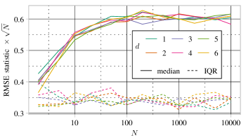
Figure 3: Median and inter-quartile range (IQR) of the RMSE of Algorithm 2

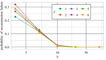
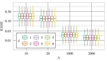
Figure 4: Probability of Algorithm 2 stop due to insufficient data

Figure 5: Boxplot of the RMSE of Algorithm 2

VI Conclusion

We have proposed a novel method for reconstructing pulse signals that recur in time. The method is based on the study of the probability distribution of sample trains along curve $\mathcal{C}$. Numerical simulations have shown that the root-mean-square error of the proposed reconstruction drops with the number of pulse recurrences $N$ at the rate $N^{-\frac{1}{2}}$. The proposed algorithm can withstand small disturbances of the input data. However, it would require some modifications at the stages of curve $\mathcal{C}$ and quantile function $Q_{p,d,\tau}$ estimation to make it more robust to noisy samples. These modifications are expected to be similar to those proposed in [10] in the context of periodic signal reconstruction. Besides such adaptation, we work on extending the procedure to pulse streams consisting of pulses that vary in amplitude.

References

- [1] S. Rudresh, S. Nagesh, and C. S. Seelamantula, “Asymmetric pulse modeling for FRI sampling,” IEEE Transactions on Signal Processing, vol. 66, no. 8, pp. 2027–2040, 2018.
- [2] H. Pan, T. Blu, and M. Vetterli, “Towards generalized FRI sampling with an application to source resolution in radioastronomy,” IEEE Transactions on Signal Processing, vol. 65, no. 4, pp. 821–835, 2017.
- [3] R. Tur, Y. C. Eldar, and Z. Friedman, “Innovation rate sampling of pulse streams with application to ultrasound imaging,” IEEE Transactions on Signal Processing, vol. 59, no. 4, pp. 1827–1842, 2011.
- [4] S. K. Shastri, S. Rudresh, R. Anand, S. Nagesh, C. S. Seelamantula, and A. K. Thittai, “Axial super-resolution in ultrasound imaging with application to non-destructive evaluation,” Ultrasonics, vol. 108, p. 106183, 2020.
- [5] E. Matusiak and Y. C. Eldar, “Sub-Nyquist sampling of short pulses,” IEEE Transactions on Signal Processing, vol. 60, no. 3, pp. 1134–1148, 2012.
- [6] C. Hegde and R. G. Baraniuk, “Sampling and recovery of pulse streams,” IEEE Transactions on Signal Processing, vol. 59, no. 4, pp. 1505–1517, 2011.
- [7] M. Najjarzadeh and H. Sadjedi, “Implementation of particle swarm optimization algorithm for estimating the innovative parameters of a spike sequence from noisy samples via maximum likelihood method,” Digital Signal Processing, vol. 106, p. 102799, 2020.
- [8] G. Huang, S. Zhang, L. Chen, H. Han, and W. Lu, “Sub-Nyquist sampling system for pulse streams based on non-ideal filters,” Digital Signal Processing, vol. 123, p. 103380, 2022.
- [9] M. W. Rupniewski, “Triggerless random interleaved sampling,” in ICASSP 2020 - 2020 IEEE International Conference on Acoustics, Speech and Signal Processing (ICASSP), 2020, pp. 5605–5609.
- [10] ——, “Super-resolution of periodic signals from short sequences of samples,” in ICASSP 2021 - 2021 IEEE International Conference on Acoustics, Speech and Signal Processing (ICASSP), 2021.
- [11] ——, “Reconstruction of periodic signals from asynchronous trains of samples,” IEEE Signal Processing Letters, vol. 28, pp. 289–293, 2021.
- [12] ——, “Period and signal reconstruction from the curve of trains of samples,” IET Signal Processing, vol. 16, no. 2, pp. 232–237, nov 2021.
- [13] T. Dey, K. Mehlhorn, and E. Ramos, “Curve reconstruction: Connecting dots with good reason,” Computational Geometry: Theory and Applications, vol. 15, no. 4, pp. 229–244, 2000.
- [14] T. Lenz, “Simple reconstruction of non-simple curves,” Freie Universitat Berlin, Tech. Rep. B 05-02, 2005.