Numerical wetting benchmarks - advancing the plicRDF-isoAdvector unstructured Volume-of-Fluid (VOF) method

Abstract

The numerical simulation of wetting and dewetting of geometrically complex surfaces benefits from unstructured numerical methods because they discretize the domain with second-order accuracy. A recently developed unstructured geometric Volume-of-Fluid (VOF) method, the plicRDF-isoAdvector method, is chosen to investigate wetting processes because of its volume conservation property and high computational efficiency. The present work verifies and validates the plicRDF-isoAdvector method for wetting problems. We present four verification studies. The first study investigates the accuracy of the interface advection near walls. The method is further investigated for the spreading of droplets on a flat and a spherical surface, respectively, for which excellent agreement with the reference solutions is obtained. Furthermore, a 2D capillary rise is considered, and a benchmark comparison based on results from previous work is performed. The benchmark suite, input data, and Jupyter Notebooks used in this study are publicly available to facilitate further research and comparison with other numerical codes.

1 Introduction

The wetting of a solid surface by a liquid is encountered in many natural and technical processes, including the spreading of paint, ink, lubricant, dye, or pesticides. In many of the typical applications, the solid surface is not flat and homogeneous but shows geometrically complex structures, chemical heterogeneity or porosity. In particular, it has been demonstrated extensively [1] that features like surface structure and roughness can be used as a tool to significantly enhance the process performance. A good example is the increase in heat transfer in boiling using textured surfaces [2]. In order to describe and predict wetting processes on complex surfaces, it is necessary to develop simulation tools that can handle the complex geometry of the boundary, strong deformations of the fluid interface, as well as separation and merging of fluid structures.
The two most well-known simulation methods for multiphase flows that naturally handle these requirements are the unstructured Volume of Fluid (VOF) method (cf. [3] for a recent review) and the Level Set method (cf. [4, 5] for recent reviews). In this study, we have chosen the Volume of Fluid (VOF) method because it is widely used for two-phase flows in technical systems and since it allows for highly accurate conservation of phase-specific volumes based on the use of a phase indicator function.

The unstructured VOF method can be classified into two categories regarding the underlying approach for the advection of volume fractions, i.e., the discretized version of the phase indicator function - algebraic and geometric VOF methods. Algebraic VOF methods solve a linear algebraic system for the advection of the volume fraction field. A well-known OpenFOAM [6] solver that uses the algebraic VOF method is interFoam [7]. Although computationally very efficient, algebraic VOF methods may lead to inaccurate results [7, 8] caused by artificial diffusion of the interface. On the other hand, geometric VOF methods reconstruct the fluid interface to approximate the phase-specific volumes fluxed through each face of the cell (see [3] for a recent review). A face-based fluxed volume can be obtained using either geometric volume calculation or the Reynolds transport theorem to compute the rate of change of volume passing through each face. The latter approach is underlying the plicRDF-isoAdvector geometric VOF method [8, 9] developed by Roenby et al. [8].

The plicRDF-isoAdvector method is based on geometric approximations both in the interface reconstruction step and in the interface advection step (cf. section 2). It achieves second-order convergence of the geometrical VOF advection error in the $L_{1}$-norm on unstructured meshes for time steps restricted to CFL numbers below $0.2$  [9]. Gamet et al. [10] have validated the plicRDF-isoAdvector method for rising bubbles and benchmarked it against interFoam [7], Basilisk [11] and results from the Finite Element Methods available in the existing literature (TP2D [12, 13], FreeLIFE [14], and MooNMD [15]). In particular, the plicRDF-isoAdvector method performed better than interFoam in capturing the helical trajectory and shape of the bubble for surface tension dominant flow. Siriano et al. [16] have tested the numerical method for rising bubbles with high-density ratios. These studies show that the plicRDF-isoAdvector method is an efficient and accurate unstructured geometrical VOF method for two-phase flow problems.

In order to verify and validate the plicRDF-isoAdvector method’s suitability for wetting problems, we investigated its performance in four test cases. The first case study is the near-wall interface advection verification test proposed by Fricke et al. [17]. It investigates the numerical contact angle evolution when the interface is advected using a known divergence-free velocity field. The results are presented in section 3.

Next, droplet spreading on a flat surface is considered - a classical wetting validation case study. Dupont and Legendre [18], and Fricke et al. [19] have studied the droplet shape with stationary geometrical relations. The droplet spreading with and without the influence of gravity is also studied. The results are presented in section 4.

Subsequently, droplet spreading on a spherical surface [20] is considered for testing the accuracy of the plicRDF-isoAdvector method on unstructured near-wall refined meshes for a geometrically more complex surface. The results are presented in section 5.

Lastly, in line with Gründing et al. [21], we study the transient capillary rise based on full continuum mechanical simulations. Here, the Navier slip condition is used as a regularization of the moving contact line singularity described by Huh and Scriven [22]. Gründing et al. [21] show that both the dimensionless group identified in [23, 24], and the Navier slip length have a major impact on the rise dynamics. The present study compares the simulation results for the capillary rise dynamics with the data from [21]. The results are presented in section 6.

For all four case studies, the input data, the primary data, the secondary data, and the post-processing utilities are publicly available online [25, 26]. The post-processing, based on Jupyter notebooks [27], simplifies the verification/validation of wetting processes, not just for OpenFOAM, but for any other simulation software, provided the files storing the secondary data (error norms) are organized as described in the README.md file [28].

This study uses the ESI OpenFOAM version (git tag OpenFOAM-v2112) [29]. The solver interFlow from the TwoPhaseFlow OpenFOAM project [30] (branch of2112) is used for the plicRDF-isoAdvector method. A python library, PyFoam [31], version 2021.6, has been used for setting up parameter studies. For initialization of the droplet, the volume fraction field is computed using the Surface-Mesh/Cell Approximation Algorithm (SMCA) [32] and exact implicit surfaces. An OpenFOAM submodule, cfMesh [33], is employed for discretizing the domain using unstructured meshes. An open-source software, FreeCAD [34], version 0.18.4, is used to create .stl files.

2 Numerical method

In this section, we provide an overview of the plicRDF-isoAdvector numerical method [9, 30].

2.1 Volume-of-Fluid method

Consider a physical domain $\Omega$ as illustrated in fig. 1, composed of two sub-domains occupied with different incompressible fluids, denoted by $\Omega^{+}(t)$ and $\Omega^{-}(t)$.

Figure 1: Schematic diagram of a multiphase domain $\Omega$ with contact line $\Gamma(t)$. The interface $\Sigma(t)$ intersects the solid domain boundary $\partial\Omega_{wall}$ at the contact angle $\theta$.

The phase-indicator function

$$\chi(t,\textbf{x})=\begin{cases}1&\textbf{x}\in\Omega^{+}(t)\\ 0&\textbf{x}\notin\Omega^{+}(t)\end{cases}$$ (1)

distinguishes the sub-domains $\Omega^{\pm}$. Evidently, the sub-domain $\Omega^{+}$ is then

$$\Omega^{+}(t):=\{\textbf{x}\in\Omega:\chi(t,\textbf{x})=1\}.$$ (2)

The volume fraction $\alpha_{c}(t)$ of the phase $\Omega^{+}(t)$ inside a fixed control volume $\Omega_{c}$ at time $t$ is defined as

$$\alpha_{c}(t):=\frac{1}{|\Omega_{c}|}\int_{\Omega_{c}}\chi(t,\textbf{x})\,dV\,.$$ (3)

The value of the volume fraction inside a cell indicates whether phase $\Omega^{+}(t)$ is present inside the cell. Indeed, it holds that

$$\begin{split}\alpha_{c}=1&\Longleftrightarrow\text{cell is inside }\Omega^{+}(t),\\ \alpha_{c}\in(0,1)&\Longleftrightarrow\text{cell intersects the interface (``interface cell")},\\ \alpha_{c}=0&\Longleftrightarrow\text{cell is inside }\Omega^{-}(t).\end{split}$$ (4)

Within each phase $\Omega^{+}(t)$ or $\Omega^{-}(t)$, mass conservation for incompressible fluids has the form of

$$\nabla\cdot\mathbf{v}=0,$$ (5)

where $\mathbf{v}$ is the fluid velocity. In situations without phase change, the phase indicator function keeps its value along trajectories of the two-phase flow, i.e., it satisfies (in a distributional sense) the transport equation

$$\partial_{t}\chi+{\bf v}\cdot\nabla\chi=0.$$ (6)

The phase-indicator $\chi(t,\cdot)$ determines the phase-dependent local values of the physical quantities such as the single-field density $\rho$ and viscosity $\mu$ in the single-field formulation of the two-phase Navier Stokes equations. For constant densities $\rho^{+}$, $\rho^{-}$ and constant viscosities $\mu^{+}$, $\mu^{-}$, we have

$$\rho(t,\mathbf{x})=\chi(t,\mathbf{x})\rho^{+}+(1-\chi(t,\mathbf{x}))\rho^{-},$$ (7)

and

$$\mu(t,\mathbf{x})=\chi(t,\mathbf{x})\mu^{+}+(1-\chi(t,\mathbf{x}))\mu^{-}.$$ (8)

The momentum balance reads as

$$\partial_{t}(\rho\mathbf{v})+\nabla\cdot(\rho\mathbf{v}\mathbf{v})=-\nabla p+\nabla\cdot\left(\mu(\nabla\mathbf{v}+\nabla\mathbf{v}^{T})\right)+\rho\textbf{g}+\mathbf{f}_{\Sigma},$$ (9)

where $p$ is pressure, g is gravitational acceleration, and $\mathbf{f}_{\Sigma}=\sigma\kappa\mathbf{n}_{\Sigma}\delta_{\Sigma}$.

The VOF methods integrate eq. 6 over a fixed control volume $\Omega_{c}$ within a time step $[t^{n},t^{n+1}]$, followed by the application of the Reynolds transport theorem. This leads to the integral form of the volume fraction transport equation (see [3] for details) according to

$$\alpha_{c}(t^{n+1})=\alpha_{c}(t^{n})-\frac{1}{|\Omega_{c}|}\int_{t^{n}}^{t^{n+1}}\int_{\partial\Omega_{c}}\chi(t,\textbf{x})\mathbf{v}\cdot\mathbf{n}\leavevmode\nobreak\ dS\leavevmode\nobreak\ dt.$$ (10)

The boundary $\partial\Omega_{c}$ of the cell $\Omega_{c}$, used on the r.h.s. of eq. 10, is a union of surfaces (faces) that are bounded by line segments (edges), namely

$$\partial\Omega_{c}=\cup_{f\in F_{c}}S_{f}.$$ (11)

Using this decomposition (eq. 11) of $\partial\Omega_{c}$, eq. 10 can be written as

$$\alpha_{c}(t^{n+1})=\alpha_{c}(t^{n})-\frac{1}{|\Omega_{c}|}\sum_{f\in F_{c}}\int_{t^{n}}^{t^{n+1}}\int_{S_{f}}\chi(t,\textbf{x})\mathbf{v}\cdot\mathbf{n}\leavevmode\nobreak\ dS\leavevmode\nobreak\ dt.$$ (12)

The double integral on the right-hand side of eq. 12 defines the amount of the phase-specific volume $|V_{f}^{\alpha}|$ fluxed over the face $S_{f}$ within a time interval $[t^{n},t^{n+1}]$. Equation 12 is still an exact equation since no approximations have been made so far. It is the basis for every geometric VOF method [3], that all obtain the form,

$$\alpha_{c}(t^{n+1})=\alpha_{c}(t^{n})-\frac{1}{|\Omega_{c}|}\sum_{f\in F_{c}}V_{f}^{\alpha},$$ (13)

differing only in how $V_{f}^{\alpha}$ - the fluxed phase-specific volume - is calculated. If one could calculate $V_{f}^{\alpha}$ exactly for arbitrary $\mathbf{v}$ and $\chi$, and exactly represent the domain boundary $\bigcup_{c\in C}\partial\Omega_{c}$, eq. 13 would be an exact equation.

2.2 The plicRDF-isoAdvector method

Geometric VOF methods rely on a cell-based geometrical approximation of the interface. Each interface reconstruction algorithm thus aims to accurately compute the interface normal $\mathbf{n}_{\Sigma,c}$ and position $\mathbf{x}_{\Sigma,c}$. At first, the interface orientation algorithm approximates $\mathbf{n}_{\Sigma,c}$. Then the interface positioning algorithm places the interface at $\mathbf{x}_{\Sigma,c}$. The well-known Piecewise Linear Interface Calculation (PLIC) algorithm is the common interface reconstruction algorithm. The Youngs’ algorithm [35], the Least Squares Fit (LSF) algorithm [36], and the plicRDF reconstruction method [9] are a few examples of the PLIC-based interface orientation algorithms.

The plicRDF reconstruction method [9] is an iterative variant of the Reconstructed Distance Function (RDF) method [37], which reconstructs the so-called signed distance functions (RDFs), and normals can be approximated as a discrete gradient of the RDFs. The method iteratively updates the approximated normals, and the residual stopping criterion is applied to minimize the number of reconstruction algorithm iterations. The plicRDF method estimates the initial interface normal in the first time step as

$$\mathbf{n}^{k=0}_{\Sigma,c}\equiv\mathbf{n}_{\Sigma,c}(t=0)\approx\frac{\nabla_{c}\alpha_{c}}{|\nabla_{c}\alpha_{c}|},$$ (14)

where $\nabla_{c}$ is the discrete unstructured Finite Volume least squares gradient. The initial interface-normal estimates are used by a PLIC positioning algorithm (e.g., [38]) to place the interface, resulting in PLIC centroid positions $\{\mathbf{x}_{\Sigma,i}^{k=0}\}_{i\in I}$ - with $I$ as the cell-local index set of all interface-cells. For time steps $n>1$, the estimate of $\mathbf{n}_{\Sigma,c}^{k=0}$ in the cell $\Omega_{c}$ is based on the weighted average of the interface-normal values $\{\mathbf{n}_{\Sigma,l}^{n-1}\}_{l\in N_{c}}$ from the previous time-step ($t^{n-1}$), associated with the interface cells $\{\Omega_{\Sigma,l}\}_{l\in N_{c}}$ in the point-neighborhood of $\Omega_{c}$, given by the cell-local index set $N_{c}$, and is obtained as

$$\mathbf{n}_{\Sigma,c}^{k=0}=\frac{\sum_{l}w_{l}^{k=0}\mathbf{n}_{\Sigma,l}^{n-1}}{\sum_{\tilde{l}}w_{\tilde{l}}^{k=0}},$$ (15)

and the weights are calculated using a Semi-Lagrangian method as

$$w_{l}^{k=0}=\left|\mathbf{n}_{\Sigma,l}^{n-1}\cdot[(\mathbf{x}_{c}-\textbf{v}_{c}\Delta t)-\textbf{x}_{\Sigma,l}^{n-1}]\right|,$$ (16)

where $\mathbf{x}_{c}$ is the centre of cell $\Omega_{c}$, and $\textbf{v}_{c}$ is the velocity in the cell $\Omega_{c}$.

Starting with an initial interface-normal estimate $\mathbf{n}_{\Sigma,c}^{k=0}$, plicRDF improves the interface-normal orientation iteratively by reconstructing the signed distance function (RDF) in the tubular neighborhood of the interface cells (cf. fig. 2).

Figure 2: The reconstructed signed distance function field for a droplet.

The RDF $\Psi_{c}$ reconstructed at the centroid $\mathbf{x}_{c}$ of the finite volume $\Omega_{c}$ is obtained as a weighted average of the distances $\{\tilde{\Psi}_{n}\}_{n\in N_{c}}$ associated with centroids of the cells $\{\Omega_{n}\}_{n\in N_{c}}$ in the point-neighborhood of $\Omega_{c}$ - given by the cell-index set $N_{c}$. The signed distance of the centroid $\textbf{x}_{c}$ to the interface-plane in a neighboring interface cell $\Omega_{n}$ is

$$\tilde{\Psi}_{c}^{k}=\textbf{n}^{k}_{\Sigma,n}\cdot(\textbf{x}_{c}-\textbf{x}^{k}_{\Sigma,n}).$$ (17)

From these distances, the RDF in the centre of the cell $\Omega_{c}$ is obtained as

$$\Psi_{c}^{k}=\frac{\sum_{n}w_{n}^{k}\tilde{\Psi}^{k}_{n}}{\sum_{n}w_{n}^{k}},$$ (18)

with weights calculated as

$$w_{n}^{k}=\frac{|\textbf{n}^{k}_{\Sigma,n}\cdot(\textbf{x}_{c}-\textbf{x}^{k}_{\Sigma,n})|^{2}}{|\textbf{x}_{c}-\textbf{x}_{\Sigma,n}^{k})|^{2}}.$$ (19)

The Least Squares Finite Volume gradient of the RDF is used to update the interface-normals

$$\textbf{n}^{k+1}_{\Sigma,c}=\frac{\nabla_{c}\Psi_{c}^{k}}{\|\nabla_{c}\Psi^{k}_{c}\|},$$ (20)

where $k=1,\dots,5$ is used in [9]. The interface positioning algorithm uses $\{\mathbf{n}^{k+1}_{\Sigma,n}\}_{n\in I}$ to position the PLIC interface planes, resulting in $\{\mathbf{x}^{k+1}_{\Sigma,n}\}_{n\in I}$ needed for the next iteration.

2.2.1 The isoAdvector advection scheme

The isoAdvector numerical method [8] calculates the phase-specific fluxed volume $V_{f}^{\alpha}$ as

$$V_{f}^{\alpha} =\int_{t^{n}}^{t^{n+1}}\int_{S_{f}}\chi(t,\textbf{x})\mathbf{v}\cdot\mathbf{n}\leavevmode\nobreak\ dS\leavevmode\nobreak\ dt=\int_{t^{n}}^{t^{n+1}}\mathbf{v}_{f}(t)\cdot\hat{\mathbf{n}}_{f}\int_{S_{f}}\chi(t,\textbf{x})\leavevmode\nobreak\ dS\leavevmode\nobreak\ dt+O(h^{2})$$ (21)

$$=\int_{t^{n}}^{t^{n+1}}\frac{F_{f}(t)}{|S_{f}|}\int_{S_{f}}\chi(t,\textbf{x})\leavevmode\nobreak\ dS\leavevmode\nobreak\ dt+O(h^{2})$$

$$=\frac{0.5(F_{f}^{n}+F_{f}^{n+1})}{|S_{f}|}\int_{t^{n}}^{t^{n+1}}\int_{S_{f}}\chi(t,\textbf{x})\leavevmode\nobreak\ dS\leavevmode\nobreak\ dt+O(\Delta t^{2})+O(h^{2})$$

with velocity $\mathbf{v}_{f}(t)$ as the face-centered velocity resulting in $O(h^{2})$, defining $F_{f}\coloneqq\mathbf{v}_{f}\cdot\mathbf{n}_{f}|S_{f}|$, the volumetric flux across the face $S_{f}$. The vector $\mathbf{n}_{f}$ is the unit-normal vector of the face $S_{f}$. For a fixed prescribed velocity (for example, for the purpose of verifying advection), the velocity $\mathbf{v}_{f}$ is directly known. Otherwise, it is obtained from the solution of the Navier Stokes Equation, as detailed in [39].

The isoAdvector scheme geometrically evaluates the integral

$$\int_{t^{n}}^{t^{n+1}}\int_{S_{f}}\chi(t,\textbf{x})\leavevmode\nobreak\ dS\leavevmode\nobreak\ dt=\int_{t^{n}}^{t^{n+1}}A_{f}(t)\leavevmode\nobreak\ dt,$$ (22)

where $A_{f}(t)$ is the instantaneous face-area submerged in $\Omega^{+}(t)$ at time $t$. Details on the submerged face-area integration are available in [8].

With the calculation of the phase-specific fluxed volume $V_{f}^{\alpha}$, the cell volume fraction value is updated using eq. 13. The isoAdvector scheme restores strict boundedness $\alpha_{c}\in[0,1]$ by redistributing over-and-undershoots in $\alpha_{c}$ in the upwind direction.

2.2.2 Boundary conditions at the solid boundary

In the following, we work in the frame of reference where the solid boundary $\partial\Omega$ is at rest. We assume the boundary of the domain to be impermeable, i.e.,

$$\mathbf{v}_{\perp}\left.\right|_{\partial\Omega}=0,$$ (23)

where $\mathbf{v}_{\perp}$ is the velocity component normal to the boundary. The Navier slip boundary condition (for a flat boundary) is given as

$$\left.\mathbf{v}_{\parallel}\right|_{\partial\Omega}=\lambda\left.\frac{\partial\mathbf{v}_{\parallel}}{\partial y}\right|_{\partial\Omega},$$ (24)

where $\mathbf{v}_{||}$ is the velocity component tangential to the boundary, $\lambda$ is the slip length, and $\frac{\partial\mathbf{v}_{\parallel}}{\partial y}$ is the velocity gradient in the wall-normal direction $y$. Note that the no-slip boundary condition, i.e.,

$$\mathbf{v}_{||}\left.\right|_{\partial\Omega}=0,$$ (25)

is recovered from eq. 24 for $\lambda=0$. In this study, we apply the impermeability condition (23) together with either the Navier slip (eq. 24) or the no-slip (eq. 25) condition.

It is important to note that for the no-slip case, the numerical method relies on the so-called “numerical slip” [40] to move the contact line. The numerical slip is an inherent property of the advection algorithm, which uses the face-centred velocity to transport the volume fraction field. The face-centred velocity at the boundary cell is not strictly zero and therefore allows for the motion of the contact line. Since the amount of numerical slip is related to the mesh size, one will typically find a mesh dependence of the contact line speed if a numerical slip is used. On the other hand, mesh convergence of the contact line speed can be reached with the Navier slip condition provided that the slip length $\lambda$ is resolved by the mesh (see Section 6).

2.2.3 Boundary condition at the contact line

At the contact line, i.e., the region where the interface touches the domain boundary, the contact angle $\theta$ (see fig. 1) is defined by the geometric relation

$$\cos\theta=\mathbf{n}_{\Sigma}\cdot\mathbf{n}_{\partial\Omega},$$ (26)

where $\mathbf{n}_{\Sigma}$ is the interface unit normal and $\mathbf{n}_{\partial\Omega}$ is the outer unit normal vector of the domain boundary $\partial\Omega$. In this paper, for simplicity, the contact angle $\theta$ is always prescribed as the equilibrium contact angle.

For the numerical treatment of boundary interface cells $\Omega_{c}$, Scheufler and Roenby [41] have introduced the concept of a ghost interface point $\textbf{x}_{G,c}$ placed on the opposite side of the boundary face $b$ of the cell $\Omega_{c}$ (fig. 3). It is the unique point at a distance of $2\Delta x$ from the PLIC centroid position $\textbf{x}_{\Sigma,c}$ such that the ghost interface normal $\textbf{n}_{G,c}$ becomes oriented in such a way that it satisfies the contact angle boundary condition. In order to transmit this information about the contact angle into the algorithm, the point $\textbf{x}_{G,c}$ and the normal $\textbf{n}_{G,c}$ are then used as an additional contribution in eq. 19 to reconstruct the RDF using eq. 18 at the centroid $\mathbf{x}_{c}$ of the cell $\Omega_{c}$.

Figure 3: Contact angle treatment by the plicRDF-isoAdvector method. The ghost interface point $\textbf{x}_{G,c}$ with ghost interface normal $\textbf{n}_{G,c}$ satisfies the contact angle boundary condition and is used as an additional contribution in eq. 19 to reconstruct the RDF at the centroid $\mathbf{x}_{c}$ of cell $\Omega_{c}$.

2.2.4 The curvature model

For the curvature calculation in the interface cell $\Omega_{c}$, we have used the parabolic fit curvature model [41]. A surface given by a quadratic form is computed by fitting it to the PLIC centroids $\{\mathbf{x}_{\Sigma,n}\}_{n\in N_{c}}$ inside all neighboring interface-cells. The curvature of the surface is then approximated by the one of the quadratic surface.

Of the curvature models evaluated, the parabolic fit has shown better performance. The simulation results obtained with an arbitrarily chosen slip length and using the height function and RDF curvature models [41] are publicly available online [42, 43, 44].

3 Verification of the advection accuracy near the contact line

3.1 Definition of case study

In this study, we consider the advection of the droplet interface using a divergence-free velocity field and report the accuracy of the interface advection near walls. It has been shown in [45, 46] that the contact line advection problem is a well-posed initial value problem if the velocity field is sufficiently regular and tangential to the domain boundary. The interface motion and the contact angle evolution can be computed from the velocity field and the initial geometry. Notably, the full time evolution of the contact angle can be inferred from the solution of a system of ordinary differential equations [45]. In this study, we replicate one of the case studies presented in Fricke et al. [17].

Figure 4: Kinematic transport of the contact angle.

Kinematics of contact angle transport:

In the following, we will study the time-evolution of the contact angle along a flow trajectory $\mathbf{x}(t)$ defined as the solution of the initial value problem

$$\dot{\mathbf{x}}(t;t_{0},x_{0})=\textbf{v}(t,\textbf{x}(t;t_{0},x_{0})),\leavevmode\nobreak\ \textbf{x}(t_{0};t_{0},x_{0})=\textbf{x}_{0}.$$ (27)

We may also write $\mathbf{x}(t)$ for short, keeping in mind that an initial position must be specified. It has been shown in [45] that the contact line is invariant with respect to the flow generated by (27) provided that $\mathbf{v}$ is tangential, i.e., if $\mathbf{v}_{\bot}=0$ at the solid boundary. This means that a trajectory that starts at the contact line will always stay at the contact line, and the function

$$\theta(t):=\theta(t,\mathbf{x}(t))$$

is well-defined. Mathematically, the time-evolution of the contact angle can be deduced from the time-evolution of the normal field $\mathbf{n}_{\Sigma}$ along $\mathbf{x}(t)$ via

$$\cos\theta(t,\mathbf{x}(t))=-\mathbf{n}_{\Sigma}(t,\mathbf{x}(t))\cdot\mathbf{n}_{\partial\Omega}(t,\mathbf{x}(t)),$$ (28)

where $\textbf{n}_{\partial\Omega}$ is the outer unit normal vector of the domain boundary $\partial\Omega$. The normal field along $\mathbf{x}(t)$ satisfies the evolution equation (see [45])

$$\operatorname{\frac{d}{dt}}\,\mathbf{n}_{\Sigma}(t,\mathbf{x}(t))=-P_{\Sigma}\,\nabla\mathbf{v}(t,\mathbf{x}(t))^{\sf T}\mathbf{n}_{\Sigma}(t,\mathbf{x}(t)).$$ (29)

Here $P_{\Sigma}=\mathbb{I}-(\mathbf{n}_{\Sigma}\otimes\mathbf{n}_{\Sigma})$ is the orthogonal projection onto the tangent space of $\Sigma$ at $(t,\mathbf{x}(t)$. Note that this projection appears because the $\dot{\mathbf{n}}_{\Sigma}$ must be orthogonal to $\mathbf{n}_{\Sigma}$ due to the normalization of the vector field. In practice, it may be simpler to solve the ordinary differential equation (ODE) without $P_{\Sigma}$, i.e.,

$$\dot{\bm{\nu}}(t)=-\nabla\mathbf{v}(t,\mathbf{x}(t))^{\sf T}\cdot\bm{\nu}(t),\leavevmode\nobreak\ \bm{\nu}(t_{0})=\mathbf{n}_{\Sigma}(t_{0},x_{0}),$$ (30)

and then obtain the normal field by normalization of $\bm{\nu}$ according to

$$\textbf{n}_{\Sigma}(t,\textbf{x}(t))=\frac{\bm{\nu}(t)}{\|\bm{\nu}(t)\|}.$$ (31)

It is easy to show that both methods are, in fact, equivalent.

For this case study, we follow one of the examples in [17]. The interface $\Sigma$ is advected using a velocity field called “vortex-in-a-box” given by

$$\textbf{v}(t,x_{1},x_{2})=v_{0}\cos\left(\frac{\pi t}{\tau}\right)(-\sin(\pi x_{1})\cos(\pi x_{2}),\cos(\pi x_{1})\sin(\pi x_{2})).$$ (32)

The periodicity of the field in time allows for comparing the droplet’s initial shape at $t=t_{0}$ and the shape after the time period $\tau$. If the advection problem is solved exactly, the droplet shape at $t=0$ will coincide with the shape at $t=\tau$. Otherwise, the difference in the volume fractions fields can be used to quantify the error. Moreover, the full time-evolution of the transported contact angle is obtained from the solution of the ODE system (eqs. 27, 30 and 31).

Figure 5: Initial configuration of the interface advection problem having a droplet $\Omega^{+}$ with an interface $\Sigma$ on a flat surface $\partial\Omega_{b}$. The contact angle $\theta$ is the angle formed by interface $\Sigma$ at the contact line $\Gamma$.

3.1.1 Computational setup

We consider a droplet $\Omega^{+}$ with an interface $\Sigma$ on a flat surface $\partial\Omega_{b}$ (fig. 5). The interface $\Sigma$ with a unit normal vector $\textbf{n}_{\Sigma}$ meets the domain bottom boundary $\partial\Omega_{b}$, and the intersection is called the contact line $\Gamma$. A 2D computational domain of dimensions $[1\times 0.25]$ in the xy-plane is simulated. The initial shape of the droplet is a spherical cap with a dimensionless radius of $R_{0}=0.2$, placed on the bottom boundary

$$\partial\Omega_{b}=\{(x,0):0\leq x\leq 1\}.$$ (33)

The initial position of the spherical cap is located at the coordinates $(0.4,-0.1)$, resulting in an initial contact angle

$$\theta_{0}=\cos^{-1}\left(\frac{0.1}{0.2}\right)=60^{\circ}.$$ (34)

In this study, we choose $v_{0}=0.1$, $\tau=0.2$, and ensure that the Courant number satisfies $Co=U\frac{\Delta t}{\Delta x}<0.01$. We quantify the geometrical shape error as

$$E_{1}=\sum_{c}|\alpha_{c}(\tau)-\alpha_{c}(0)|V_{c},$$ (35)

and the maximum error in the transported contact angle as

$$E_{\infty}=\text{max}_{t\in[0,T]}|\theta_{\text{num}}(t)-\theta_{\text{ref}}(t)|,$$ (36)

where $T$ is the maximum simulation time.

Remark:

For practical reasons, a no-slip boundary condition at the bottom boundary and a zero-gradient boundary condition for the volume fractions are formally specified for the solver. However, the solution is not affected since this study is only an initial value problem.

3.1.2 Simulation results

We discretized the domain using uniform meshes. Figure 6 shows the convergence of $E_{1}$ errors for the velocity field given by eq. 32. As the mesh resolution increases, the order of convergence for $E_{1}$ errors also increases (see table 1 for $E_{1}$ error values and order of convergence at different mesh resolutions).

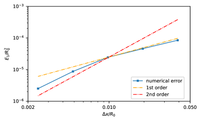
Figure 6: Convergence of $E_{1}$ errors for the velocity field (32).

Cells in x-direction	Error	Order of convergence	Error	Order of convergence
$n_{x}$	$E_{1}/R_{0}^{2}$		$E_{\infty}$ (deg)
$\mathrm{128}$	$\mathrm{8.483e-05}$		$\mathrm{2.87}$
$\mathrm{256}$	$\mathrm{4.603e-05}$	0.9216	$\mathrm{1.47}$	0.974
$\mathrm{512}$	$\mathrm{2.445e-05}$	0.9414	$\mathrm{0.77}$	0.962
$\mathrm{1024}$	$\mathrm{8.763e-06}$	1.395	$\mathrm{0.39}$	0.993
$\mathrm{2048}$	$\mathrm{2.517e-06}$	1.741	$\mathrm{0.20}$	0.948

Table 1: Error $E_{1}$ (eq. 35), error $E_{\infty}$ (eq. 36) and order of convergence.

Figure 7 show the simulation results of the numerical evolution of the transported contact angle. The solutions of the ODE (eqs. 28, 27, 30 and 31) provide the reference value of the instantaneous transported contact angle $\theta_{\text{ref}}(t)$. The numerical solution converges to the reference solution and delivers near first-order convergent results for $E_{\infty}$ (see table 1).

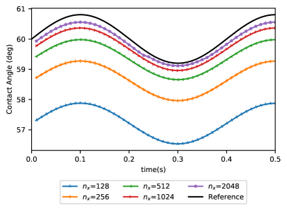
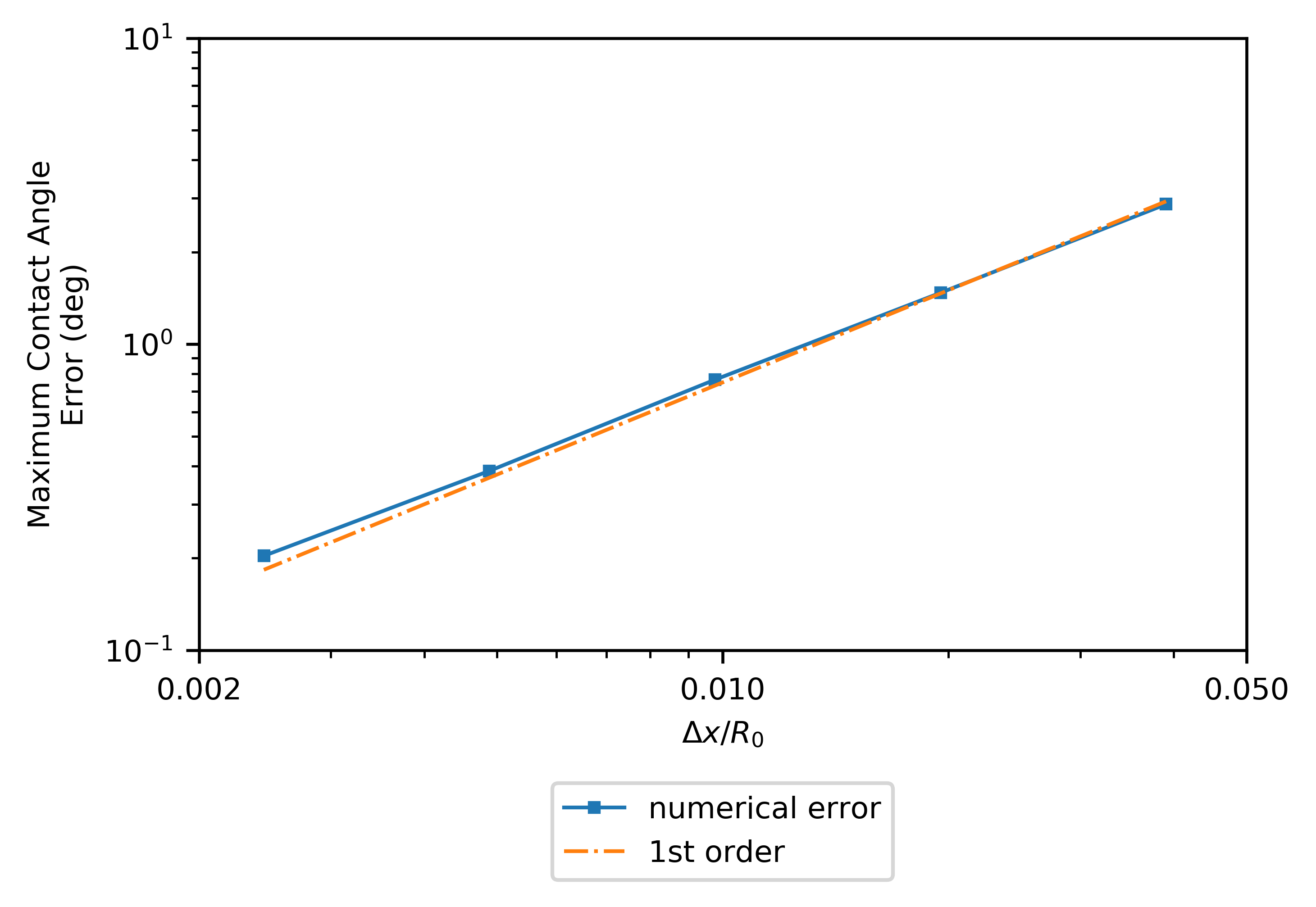
Figure 7: Left: Numerical contact angle evolution for the velocity field (eq. 32) with a uniform mesh. Right: Maximum error in the transported contact angle (eq. 36).

4 Droplet spreading on a flat surface

4.1 Definition of the case study

In this study, we investigate the spreading of a droplet on a flat surface [18]. The focus is on the effect of the static contact angle boundary condition and the Bond number, $Bo=\frac{\rho_{l}gR_{0}}{\sigma}$, on the equilibrium shape of the droplet. For a droplet that spreads with $Bo\ll 1$, the surface tension forces dominate, and the droplet at equilibrium maintains a spherical cap shape and satisfies the contact angle boundary condition. On the other hand, for $Bo\gg 1$, the gravitational forces dominate, and the droplet forms a puddle, whose height is directly proportional to the capillary length, $l_{Ca}=\sqrt{\frac{\sigma}{\rho_{l}g}}$. The droplet’s volume $V$ and the equilibrium contact angle $\theta_{e}$ are used to derive the geometrical relations for the equilibrium shape of the droplet [18, 19, 20]. Furthermore, we have also studied the mesh convergence of the spreading droplets.

Figure 8 illustrates the schematic diagram of a semi-spherical droplet initialized on a flat surface with an initial radius $R_{0}$. Note that $\theta_{0}=90^{\circ}$ is an (arbitrary) choice for the initial contact angle. The droplet spreads and attains an equilibrium state at $\theta_{e}$, having height $e$ and wetted radius $L$. The droplet wets the surface if the initial contact angle is larger than the equilibrium contact angle. Contrary to this behavior, we observe dewetting if the initial contact angle is smaller than the equilibrium contact angle.

Figure 8: Schematic diagram of initial configuration (-) of a droplet with initial radius $R_{0}$ and final equilibrium shape (--) attained by spreading on a flat surface with an equilibrium contact angle $\theta_{e}$.

We have considered droplets of water-glycerol (75% glycerol) and pure water. The viscosity of water-glycerol is larger than that of pure water by a factor of 30, while the surface tension is slightly smaller. The physical properties of both liquids are presented in table 2.

Fluid	$\rho$	$\nu$	$\sigma$
	$kgm^{-3}$	$m^{2}s^{-1}$	$Nm^{-1}$
water	$10^{3}$	$10^{-6}$	$0.072$
water-glycerol	$1194.9$	$2.51e^{-5}$	$0.0635$

Table 2: Physical parameters of the liquid droplet.

A three-dimensional computational domain (see table 3 for domain parameters) is simulated. The droplet is initialized at the center of the domain’s bottom boundary

$$\partial\Omega_{b}=\{(x,y,0):0\leq x\leq 5,0\leq y\leq 5\}.$$ (37)

Parameter	Value	Unit
Droplet initial radius, $R_{0}$	$1$	mm
Droplet initial position, $(x_{0},y_{0},z_{0})$	$(2.5,2.5,0)$	mm
Domain size	$(5,5,4)$	mm
$(n_{x},n_{y},n_{z})$	$(100,100,80)$	cells

Table 3: Computational and geometrical parameters for the droplet spreading on a flat surface with an equilibrium contact angle $\theta_{e}$.

The bottom boundary has a no-slip boundary condition for the velocity. The time step $\Delta t$ is restricted to CFL number below $0.01$.

4.1.1 Geometrical relations for a droplet at equilibrium

Droplet spreading with a very small Bond number attains a spherical cap shape at the equilibrium. The wetted radius $L$ and the height $e$ of the spherical cap are given by the geometrical relations

$$\frac{L}{V^{\frac{1}{3}}}=g(\theta)\coloneqq\sin{\theta}\left(\frac{\pi(1-\cos{\theta})^{2}(2+\cos{\theta})}{3}\right)^{-\frac{1}{3}},$$ (38)

$$e=L\tan\left(\frac{\theta}{2}\right).$$ (39)

The intersection of a spherical cap and the horizontal flat surface produces a circular contact line $\Gamma$ (see fig. 9), whose area is referred to as wetted area $A$ and can be calculated as

$$A=\pi L^{2}.$$ (40)

Figure 9: A spherical cap sitting on a flat surface.

For a droplet spreading with a large Bond number ($Bo\gg 1$), the puddle height $e$ is given by

$$e=2\sqrt{\frac{\sigma}{\rho_{l}g}}\sin\left(\frac{\theta}{2}\right).$$ (41)

The estimate for the wetted area $A$ is obtained by adding up the wetted area of each boundary face $f$, which is calculated as follows:

$$\int_{\partial\Omega}\alpha(\mathbf{x})\,ds\ =\sum_{f\in F_{c}}\alpha_{f}\|\mathbf{S_{f}}\|_{2}+O(h^{2}).$$ (42)

Here, $\alpha_{f}$ represents the volume fraction value of the boundary face, which is obtained using OpenFOAM functionalities in the function object and $\mathbf{S_{f}}$ is the face-area normal vector of the face $f$.

4.2 Spreading of a droplet with a very small Bond number

4.2.1 Convergence study

A mesh convergence study for the wetted area is conducted with four levels of mesh refinement with 10, 16, 20, and 40 cells per droplet radius. The results shown in fig. 10(a), illustrate a convergent behavior of the water-glycerol droplet with respect to the stationary state at $\theta_{e}=50$°. For a coarser mesh (cells per radius=$10$), an overshoot in the wetted area curve is observed because of the numerical dissipation being small on a coarse mesh. With numerical slip, any overshoot would disappear with mesh refinement (as observed in fig. 10(a)), as the contact line would not be able to move in the limit $\Delta x\rightarrow 0$ ($\Delta x$ is the mesh cell size). Similar convergent behavior with respect to the stationary state is observed for the water-glycerol droplet with $\theta_{e}=110$° (see fig. 10(b)). In contrast to this behavior, water droplets exhibit oscillatory spreading behavior (see  figs. 10(c) and 10(d)), taking longer to reach equilibrium, but ultimately converge towards the stationary state.

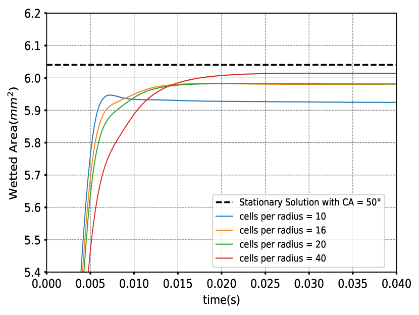
(a)

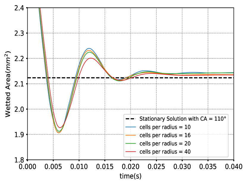
(b)

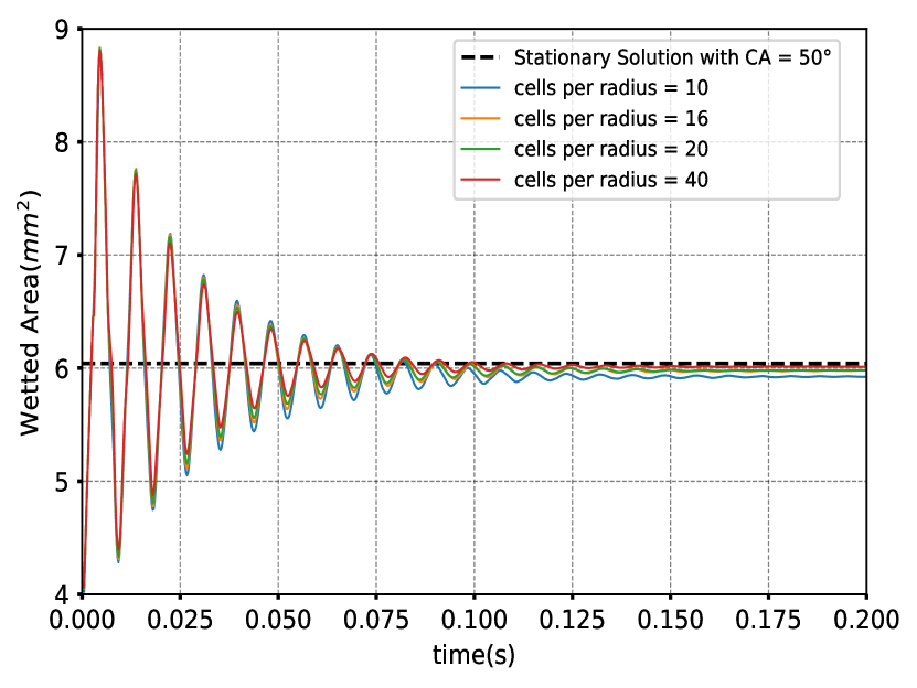
(c)

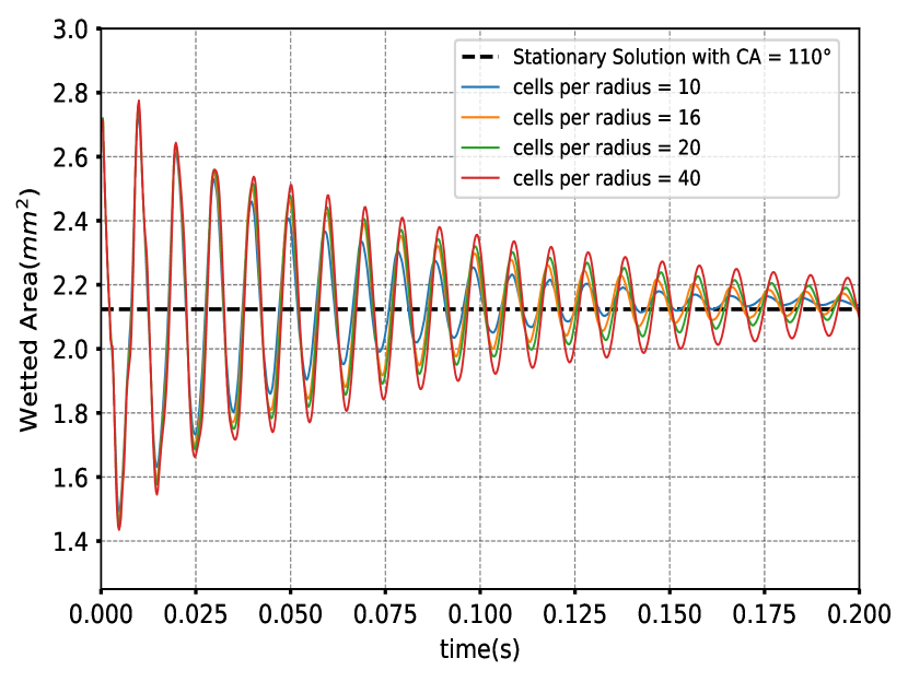
(d)

Figure 10: Convergence study of the wetted area of the spreading droplet on a flat horizontal surface. The top images (figs. 10(a), LABEL: and 10(b)) and bottom images (figs. 10(c), LABEL: and 10(d)) show the droplet spreading simulation results for water-glycerol and water droplets, respectively, with a mesh size of $10,16,20$, and $40$ cells per radius. The initial contact angle is $\theta_{0}=90$°. The equilibrium contact angles are $\theta_{e}=50$° (left, wetting) and $110$° (right, dewetting). The stationary solution (eq. 40) is represented by the dotted horizontal (black) line.

4.2.2 Geometrical characteristics of the droplet

Figure 11 illustrates the different shapes of the droplet during its spreading process. In the beginning, due to the difference between the initial and equilibrium contact angles, the droplet is far from reaching its equilibrium state, leading to a rapid movement of the contact line without any significant change in the droplet’s global shape, as depicted in fig. 11(b). As the spreading continues, the droplet’s apex velocity increases in a downward direction (fig. 11(c)), and the droplet’s overall shape starts to change until it reaches its equilibrium state (fig. 11(d)). Similar spreading behavior is reported in the literature ([47, 48, 49]).

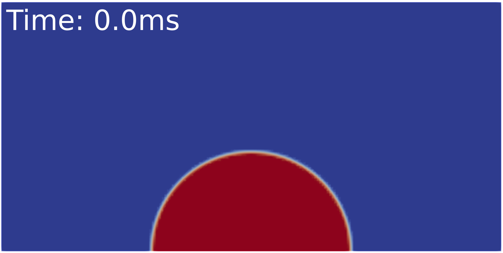
(a)

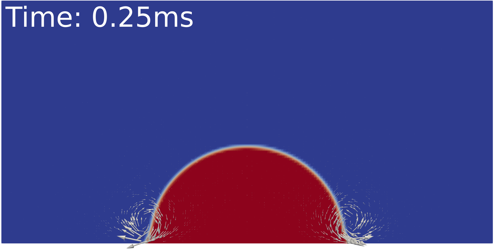
(b)

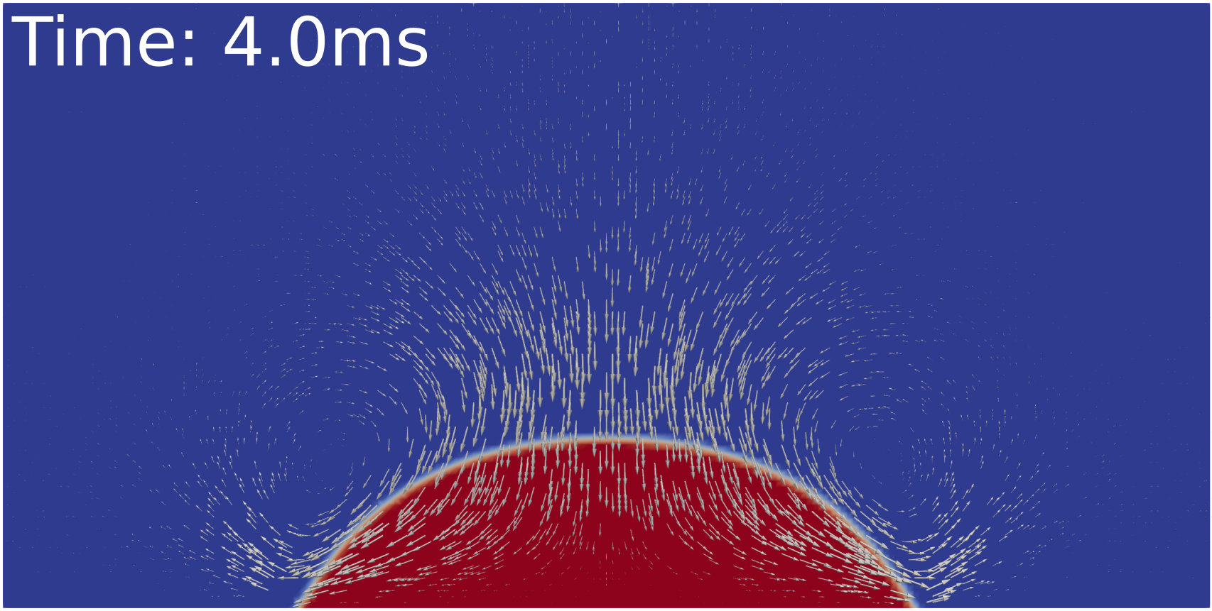
(c)

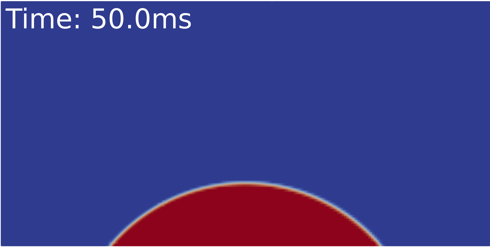
(d)

Figure 11: Simulation results of droplet spreading on a horizontal flat surface at different instants of time. The initial and equilibrium contact angles are $\theta_{0}=90$° and $\theta_{e}=50$°, respectively. The arrows represent the velocity field.

The comparison of dimensionless geometrical quantities at equilibrium with reference solutions for a range of contact angles is shown in fig. 12. The simulation results are in very good agreement with the reference solution for both hydrophilic and hydrophobic cases. We note that for the highly hydrophobic case (e.g., for $\theta_{e}=150^{\circ}$), the stationary state is not reached in a reasonable time if the droplet is initialized as a semisphere. This can be understood in terms of the initial potential energy, which is very high in the case of a semisphere (initial droplet). The quick release of this potential energy may even cause a droplet detachment from the surface. However, if the droplet is initialized closer to the equilibrium state ($\theta_{0}\approx 180^{\circ}$), convergence to the reference stationary state is observed.

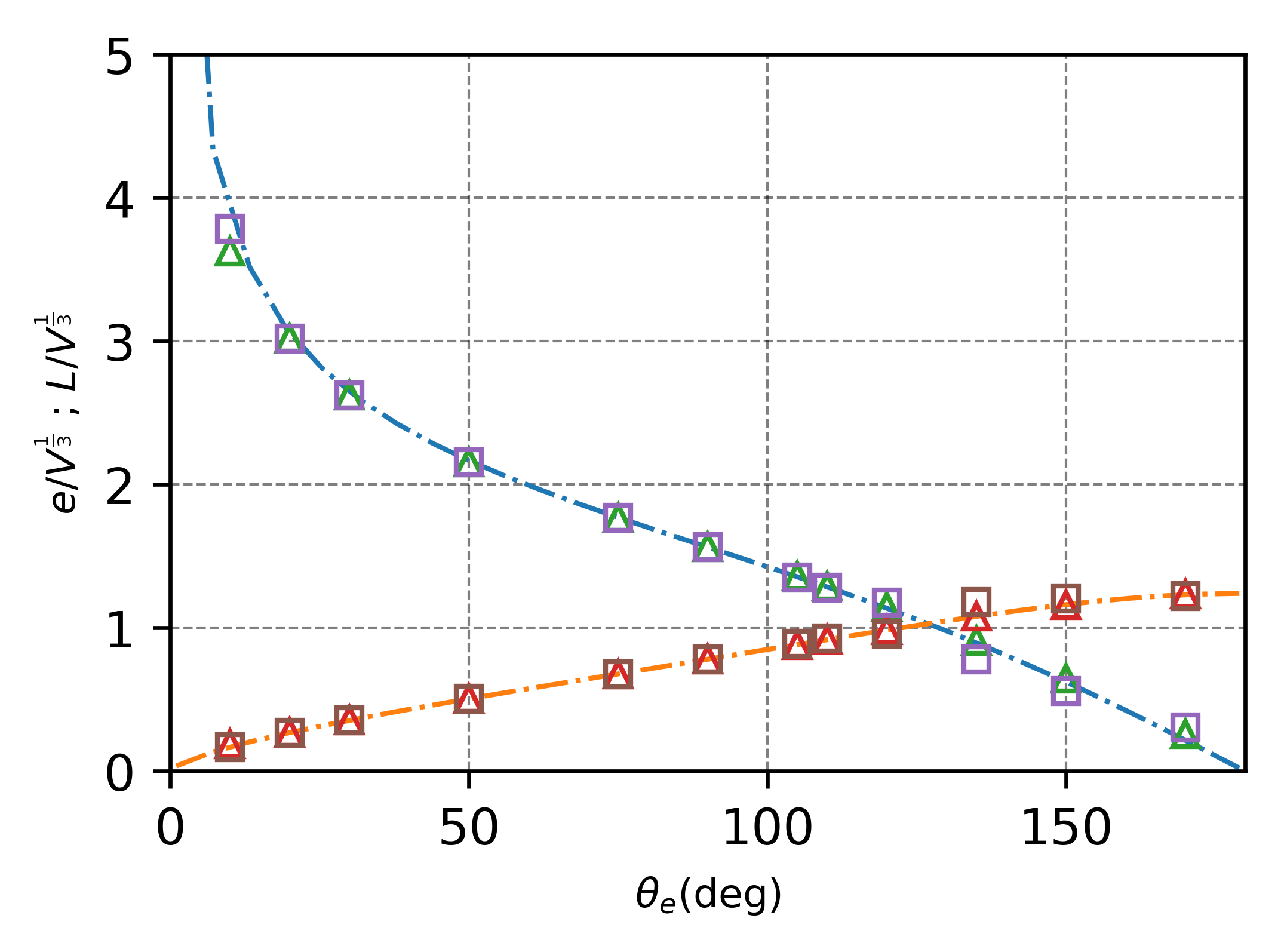
Figure 12: Droplet spreading on a horizontal flat surface: Geometrical characteristics of the droplet against the equilibrium contact angle $\theta_{e}$. wetted radius for water, equilibrium height for water, wetted radius for water-glycerol and equilibrium height for water-glycerol. The stationary solution for wetted radius (–$\cdot$–) and equilibrium droplet height (–$\cdot$–) is given by, eqs. 38, LABEL: and 39, respectively.

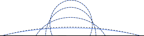
Figure 13: Droplet spreading on a horizontal flat surface: Equilibrium drop shapes for equilibrium contact angle
$\theta_{e}$ = 10°, 50°, 90°, 110°: numerical (—) and theoretical (--).

As shown in fig. 13, the equilibrium shape of the water-glycerol droplet, represented by $\alpha=0.5$ contours in ParaView [50], is compared to the reference spherical cap for a specific contact angle. The comparison illustrates that the equilibrium shape of the droplet has a very good qualitative match with the reference shape.

4.3 Spreading of a droplet with varying Bond numbers

We now consider a droplet spreading for a range of the Bond number (see table 4). Here we have two spreading behaviors - the surface tension-dominant spreading ($Bo\ll 1$) and the gravitational-dominant spreading ($Bo\gg 1$), with the transition of behavior to be observed at $Bo\approx 1$. Figure 14 shows the non-dimensional equilibrium droplet height comparison with the reference solutions in the limiting cases $Bo\rightarrow\infty$ and $Bo\rightarrow 0$. The simulation results for the spreading of the water and water-glycerol droplets are in excellent agreement with the reference solution for hydrophobic and hydrophilic cases.

Bo - water-glycerol	1e-05	1e-02	1e-01	5e-01	1	5	10
Bo - water	7.4e-06	7.4e-03	7.4e-02	3.7e-01	7.4e-01	3.7	7.4

Table 4: Range of the Bond numbers for droplets spreading on a flat surface under the influence of gravity.

Figure 14: Normalized droplet height $e^{*}$ ($e^{*}=e/e_{0}$, where $e_{0}$ is the equilibrium height at $Bo\ll 1$) on a flat surface with an equilibrium contact angle $\theta_{e}$; left: $\theta_{e}=50$°, right: $\theta_{e}=110$°.

In summary, the simulation results using the plicRDF-isoAdvector method are in excellent agreement with the reference solution in terms of mesh convergence study, droplet shape comparison, and the incorporation of gravity effects on droplet spreading. It is noted, however, that for contact angles greater than 150 degrees, the simulation results show a significant dependence on the initial conditions. This is a common issue for two-phase flow solvers when dealing with extreme contact angles $(<10^{\circ},>150^{\circ})$, as reported in [18, 20].

5 Droplet spreading on a spherical surface

5.1 Definition of the case study

This study investigates the spreading of a droplet on a complex spherical surface with a very small Bond number ($Bo\ll 1$) [20]. As discussed in section 4, a droplet that spreads with $Bo\ll 1$, maintains a spherical cap shape at the equilibrium.

A three-dimensional computational domain is simulated, with domain parameters provided in table 5. The domain is discretized using an unstructured Cartesian mesh, with a refined local mesh around the sphere and a uniform mesh size of 20 cells per radius. The droplet, with an initial radius $R_{0}$, is placed on the top of the spherical surface. The spherical surface has a no-slip boundary condition for the velocity (it applies numerical slip [40] for the motion of the contact line). The droplet spreads on the spherical surface until it reaches the equilibrium, satisfying the static contact angle boundary condition. The physical parameters of the water-glycerol droplet are provided in table 2. The time step $\Delta t$ is restricted to CFL number below $0.01$ to ensure stability.

Figure 15: Schematic diagram of the initial configuration of a droplet (--) with initial radius $R_{0}$ (left) and final equilibrium shape (--) (right) spreading on a spherical surface (–) with equilibrium contact angle $\theta_{e}$. The equilibrium height is $e$, and the contact radius is $r$.

Parameter	Value	Unit
Droplet initial radius, $R_{0}$	$1$	mm
Droplet initial position, $(x_{0},y_{0},z_{0})$	$(2.5,2.5,2.372)$	mm
Spherical surface position, $(x_{s},y_{s},z_{s})$	$(2,2,0.7)$	mm
Domain size	$(5,5,5)$	mm
$(n_{x},n_{y},n_{z})$	$(100,100,80)$	cells
Equilibrium contact angle, $\theta_{e}$	$30\text{, }50\text{, }90\text{, }110\text{, }140$	deg

Table 5: Computational and geometrical parameters for the droplet spreading on a spherical surface with given equilibrium contact angle $\theta_{e}$.

5.1.1 Geometrical relations for a droplet at equilibrium

The conservation of the droplet’s volume $V$ allows the formulation of geometrical relations for the contact radius $r$ and the droplet height $e$, which define the spherical cap at the equilibrium as

$$\begin{split}\alpha+\beta&=\theta_{e},\\ r&=R\sin\beta=R_{0}\sin\alpha,\\ e&=R(1+\cos\beta)-R_{0}(1-\cos\alpha),\\ \frac{8\pi R_{0}^{3}}{3}&=\frac{\pi R^{3}}{3}(1+\cos\beta)^{2}(2-\cos\beta)+\frac{\pi R_{0}^{3}}{3}(1+\cos\alpha)^{2}(2-\cos\alpha).\end{split}$$ (43)

Here, the unknown parameters are $\alpha,\beta,r,e,$ and $R$. With the known droplet volume $(V_{\text{exact}}=\frac{4\pi R_{0}^{3}}{3})$ and initial guess for $\alpha$ and $\beta$, an intermediate volume $V^{k}(\alpha,\beta,R_{0})$ is calculated by solving eq. 43 iteratively for $k$-iterations using the bisection method. The values of $\alpha$ and $\beta$ that minimize $|V_{\text{exact}}-V^{k}(\alpha,\beta,R_{0})|$ are then used to approximate the contact radius $r$ and droplet height $e$.

5.2 Post-processing

Figure 16 shows the droplet’s shapes at different instances during spreading. The droplet’s spreading dynamics are similar to those observed on a flat surface, as previously discussed in section 4. At the beginning of spreading, initial rapid spreading locally at the contact line is observed, as shown in fig. 16(b). As the simulation time progresses, the droplet’s apex velocity increases in the downward direction (fig. 16(c)), and the global shape of the droplet starts to change until the droplet attains the equilibrium shape (fig. 16(d)).

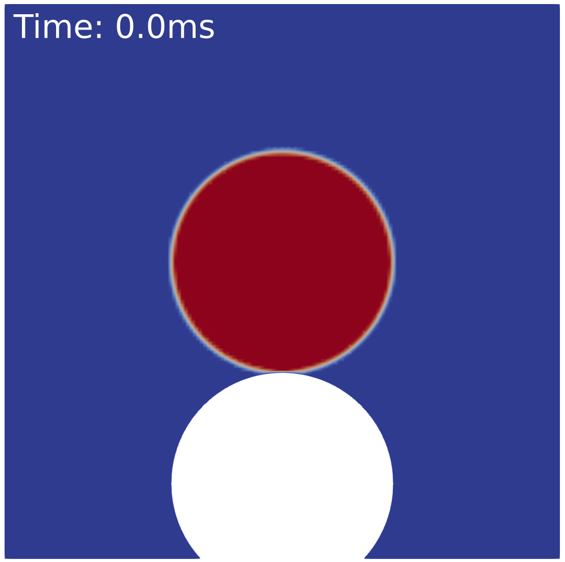
(a)

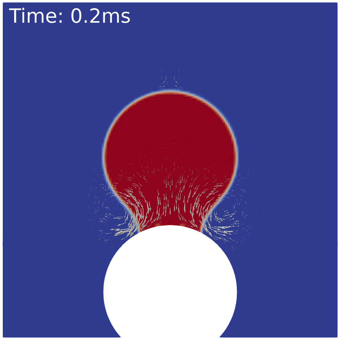
(b)

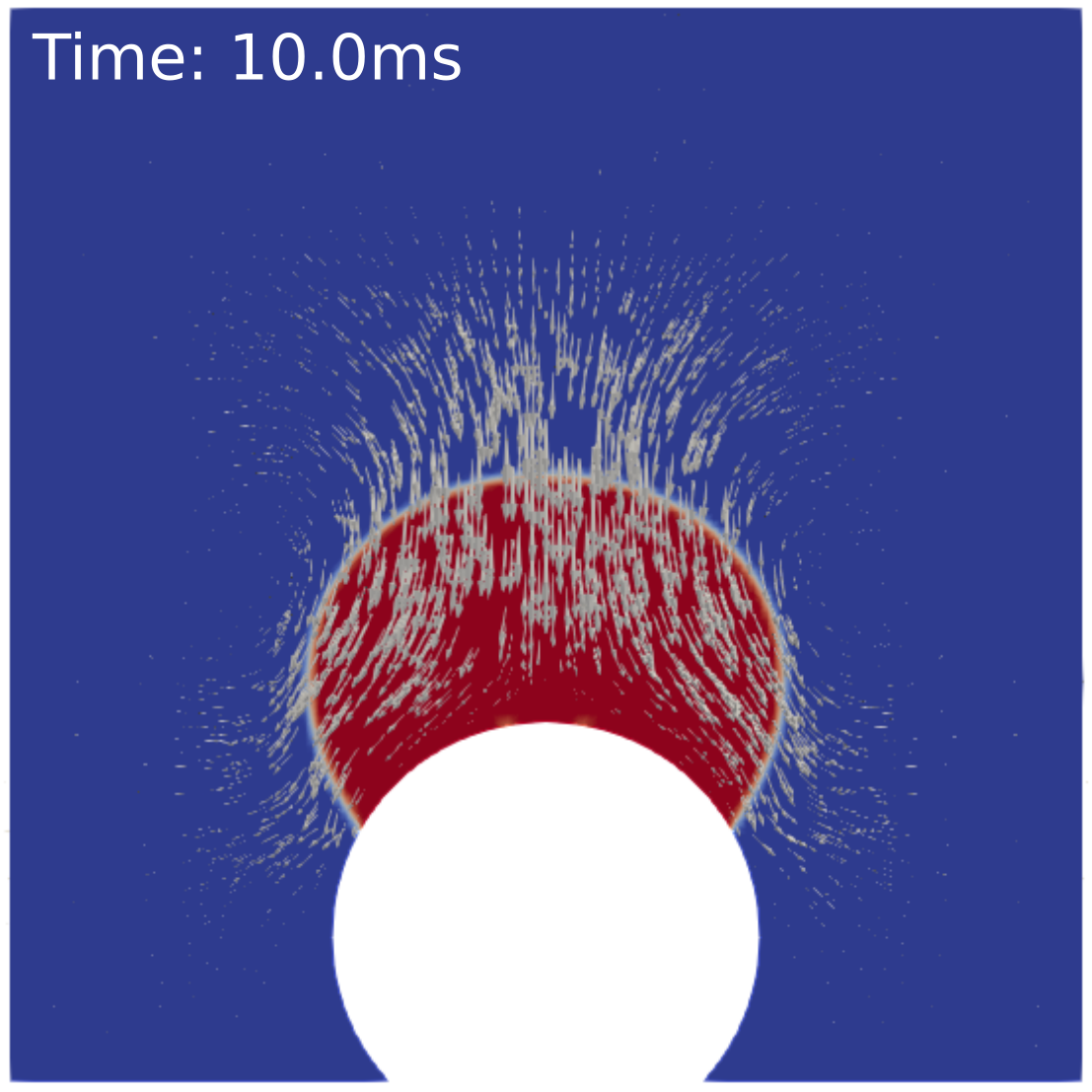
(c)

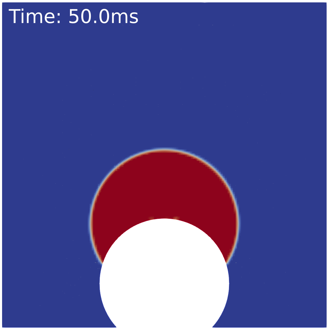
(d)

Figure 16: Simulation results of droplet spreading on a spherical surface at different instants of time. The equilibrium contact angle is $\theta_{e}=50$°. The arrows represent the velocity field.

The numerical solution of the contact radius $r$ and equilibrium height $e$ involves identifying the boundary cells that contain the contact line. The contact line position $\textbf{x}_{\Gamma}$ is determined by identifying the intersection point of the interface element $\Sigma$ and the domain boundary $\partial\Omega$ (as shown in fig. 17). To locate this point, the signed distances $\Phi_{v}$ are reconstructed at the vertices $v\in V$ of the boundary interface cells $\Omega_{c,\Sigma}$ that have $V$ vertices and $F_{c}$ faces. For a face $f\in F_{c}$ with an intersection point, the signed distance values $\Phi_{v}$ must change signs when looping over its vertices (as depicted in fig. 17). If the intersection point is within the cell, it is marked as a contact line cell, and the contact angle is subsequently calculated using the interface normal $\textbf{n}_{\Sigma}(t,\textbf{x}(t))$ and the outward unit normal vector $\textbf{n}_{\partial\Omega}$ to the boundary as

$$\theta=\cos^{-1}(\langle-\textbf{n}_{\Sigma}(t,\textbf{x}(t)),\textbf{n}_{\partial\Omega}(x(t))\rangle).$$ (44)

Identifying a contact line can be challenging due to the formation of wisps - small artificial interface elements that appear in the bulk phase (as discussed by Marić et al. [51]). To address this issue, an OpenFOAM function object was developed to detect and remove wisps from the contact line detection process.

Figure 17: Contact angle and contact line position from PLIC reconstruction. The marked cell is the interface cell at the boundary. The signed distances are calculated for each vertex of this cell. The change in signs of these distances then detects the presence of the contact line.

5.3 Geometrical characteristics of the droplet

The simulation results for the non-dimensional equilibrium contact radius and height of a droplet spreading on a spherical surface for a range of equilibrium contact angles are presented in fig. 18. These results are compared to the reference solution from eq. 43 and are in excellent agreement. The equilibrium droplet shapes for various contact angles are illustrated in fig. 19 using $\alpha=0.5$ contours. The comparison shows a good qualitative match between the reference and simulated droplet shapes.

The simulation results using the plicRDF-isoAdvector method have shown good agreement with the reference solution for droplet shape and geometrical characteristics. However, it should be noted that the symmetrical spreading of the droplet on the spherical surface is very sensitive to numerical noise. Simulations with small perturbations in the initial spherical shape can lead to a different equilibrium shape, with the droplet tilting to one side of the spherical surface. Even in such a case, the droplet shape remains close to a spherical cap, and the static contact angle boundary condition is still satisfied.

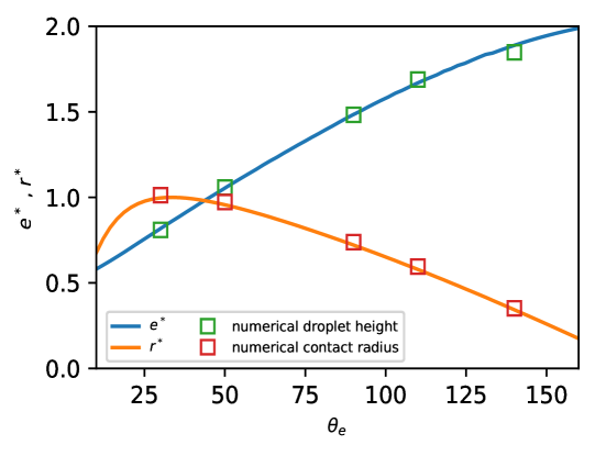
Figure 18: Dimensionless geometrical characteristics of the equilibrium droplet shape on a spherical surface: height (—), contact radius (—), numerical height ( ), numerical contact radius ( ).

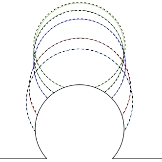
Figure 19: Equilibrium drop shapes for equilibrium contact angle $\theta_{e}$ = 30°, 50°, 90°, 110°, and 140°: geometrical reference solution (--) (eq. 43), numerical (—).

6 2D capillary rise

6.1 Definition of the case study

The process of liquid flowing through narrow spaces, known as capillary action, has been studied profoundly in the literature (see, e.g., [52, 23, 24]). The process can be observed in the distribution of water from plants’ roots to the rest of the body, the rising of liquids in porous media such as paper, and oil extraction from reservoirs, among others. In this validation study, we consider the two-dimensional case which corresponds to the rise of a liquid column between two planar parallel surfaces, as shown in [21]. We present a mesh convergence study for both the case of a no-slip (numerical slip) and a Navier slip boundary condition with a resolved slip length. As reported in [21], resolving the slip length with the computational mesh is crucial for finding the mesh convergence of the contact line dynamics. We present the comparison of the plicRDF-isoAdvector method with other numerical methods:

1. the OpenFOAM solver interTrackFoam, an Arbitrary Lagrangian-Eulerian (ALE) method.

2. the Free Surface 3D (FS3D), an in-house two-phase flow solver implying the geometric Volume-of-Fluid (VOF) method.

3. the OpenFOAM-based algebraic VOF solver, interFoam.

4. the Bounded Support Spectral Solver (BoSSS) is based on the extended discontinuous Galerkin method.

Quéré et al. [23], and Fries and Dreyer [24] study the capillary rise based on a simplified model introduced by Bosanquet [53]. The latter model is an ODE resulting from empirical modeling of the forces acting on the liquid column. It can be shown easily [23, 24] that the dynamics of the capillary rise in Bosanquet’s model is controlled by a single non-dimensionless group $\Omega$ defined as

$$\Omega=\sqrt{\frac{9\sigma\cos\theta\mu^{2}}{\rho^{3}g^{2}R^{5}}}.$$ (45)

Moreover, Quéré et al. [23] showed that Bosanquet’s model shows a regime transition at a critical value $\Omega_{c}=2$. The column approaches its stationary state monotonically for $\Omega>2$ while it shows rise height oscillations for $\Omega<2$. Notably, Gründing et al. [21] showed in their study that the Navier slip length, which is not accounted for in Bosanquet’s model, can significantly influence the rise dynamics and the transient regime. In fact, rise height oscillations are increasingly damped out as the slip length decreases. This observation led to improved ODE modeling of capillary rise, taking into account the flow near the contact line [54].

In the stationary state, the height of the liquid column can be estimated by Jurin’s law as

$$h\textsubscript{Jurin,2D}=\frac{\sigma\cos{\theta}}{R\rho g},$$ (46)

where $\sigma$ is the surface tension coefficient, $R$ is the radius of the capillary, $\rho$ is the density of the liquid, $g$ is the gravitational acceleration, and $\theta$ is the contact angle. However, equation (46) neglects the liquid volume in the interface region, hence, overestimating the true stationary rise height. Gründing et al. [21, 54] computed a corrected stationary capillary height from the liquid volume in the interface region (assuming a spherical cap shape). The corrected formula reads as

$$h=h\textsubscript{Jurin,2D}-\frac{R}{2\cos\theta}\left(2-\sin\theta-\frac{\sin^{-1}(\cos\theta)}{\cos\theta}\right).$$ (47)

6.1.1 Computational domain

The initial configuration of the two-dimensional computational domain is shown in fig. 20. The domain is discretized using the blockMesh utility of OpenFOAM, which creates a uniform Cartesian mesh in both the x and the y direction. The volume fraction field is initialized as a box $2\text{R}\times 2\text{R}$ at the bottom of the capillary. As the simulation starts, the interface evolves to satisfy the contact angle boundary condition and then rises. The set of physical parameters taken from [21] is designed to achieve different values for $\Omega$ while keeping the Bond number constant (see table 6).

Figure 20: Schematic diagram of the initial configuration of the 2D capillary rise.

$\Omega$	$R$	$\rho$	$\mu$	$g$	$\sigma$	$\theta_{e}$	Camax	Bo
-	m	$\text{kgm}^{-3}$	Pa s	$\text{ms}^{-2}$	$\text{Nm}^{-1}$	°	-	-
0.1	0.005	1663.8	0.01	1.04	0.2	30	0.0033	0.217
0.5	0.005	133.0	0.01	6.51	0.1	30	0.015	0.217
1	0.005	83.1	0.01	4.17	0.04	30	0.029	0.217

Table 6: Physical parameters for different $\Omega$.

6.2 Mesh convergence study

A mesh convergence study for the 2D capillary rise with a mesh resolution of 16 to 256 cells per diameter of the capillary was conducted. We keep $\Omega=1$ and the slip length $\lambda=0.1\leavevmode\nobreak\ \mathrm{mm}$ for this study. The simulations are done using both Navier slip and no-slip (numerical slip) boundary conditions. The results in fig. 21(a) are obtained using the no-slip boundary condition. However, since the method has some implicit “numerical slip”, we still observe a contact line motion. As a consequence of the numerical slip being linked to the grid size, the results show a strong dependence on mesh resolution regarding the dynamics. In particular, the oscillations are increasingly dampened with the increase in the mesh resolution. This is expected since, for no-slip, it is well known that the viscous dissipation near the contact is non-integrably singular. As the slip length decreases, thus approaching the no-slip limit, the numerical solution starts showing the signature of the ill-posedness of the limiting problem (Huh and Scriven paradox [22]). However, for Navier slip with positive slip length, pressure and viscous dissipation are integrable [55]. Therefore, the simulations with Navier slip (see fig. 21(b)) show mesh convergence. Although the solutions with the numerical slip and Navier slip differ in the rise dynamics, it is to be noted that the stationary rise height is mesh-independent for both cases and levels at the corrected stationary rise height (given by eq. 47).

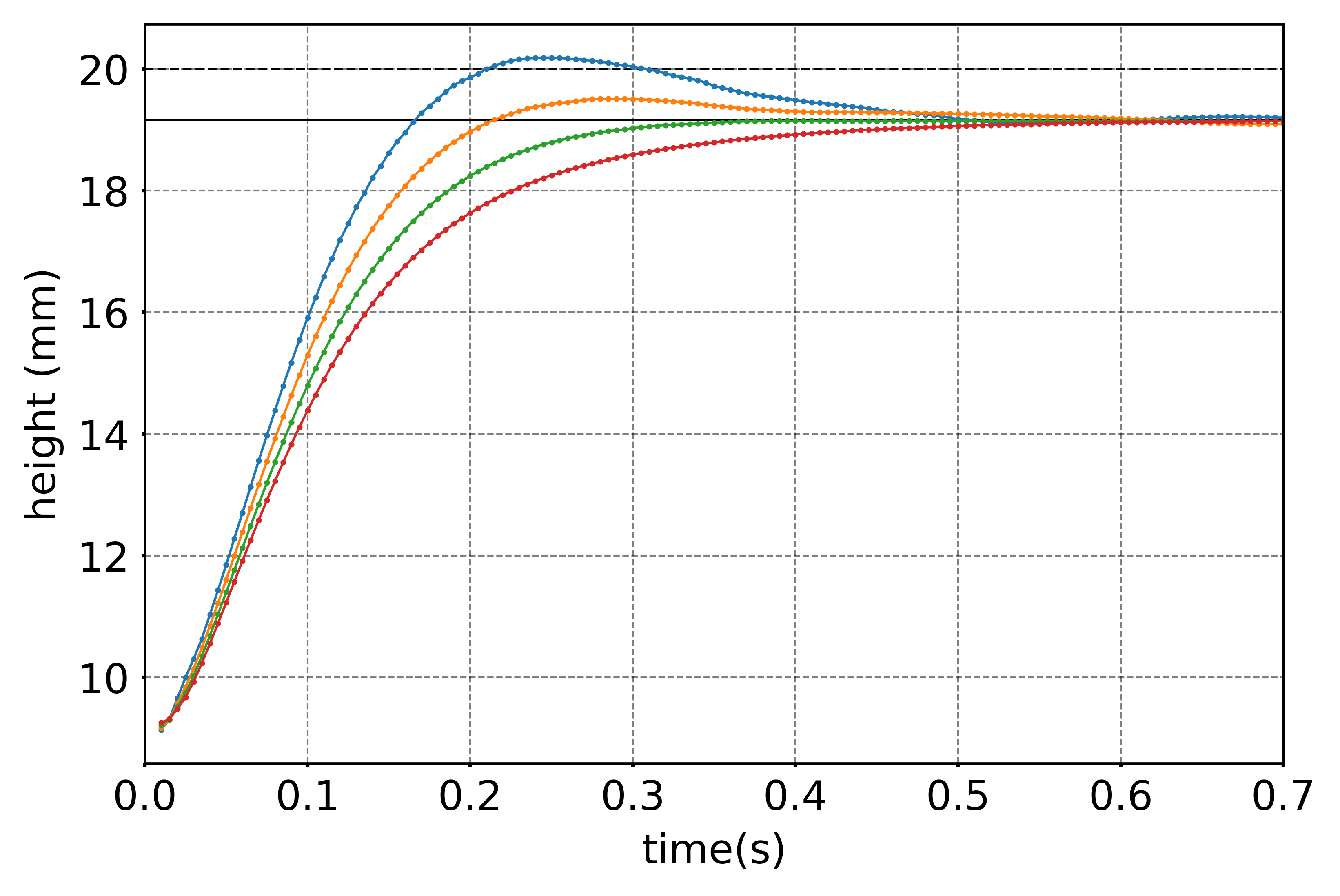
(a) No-slip boundary condition.

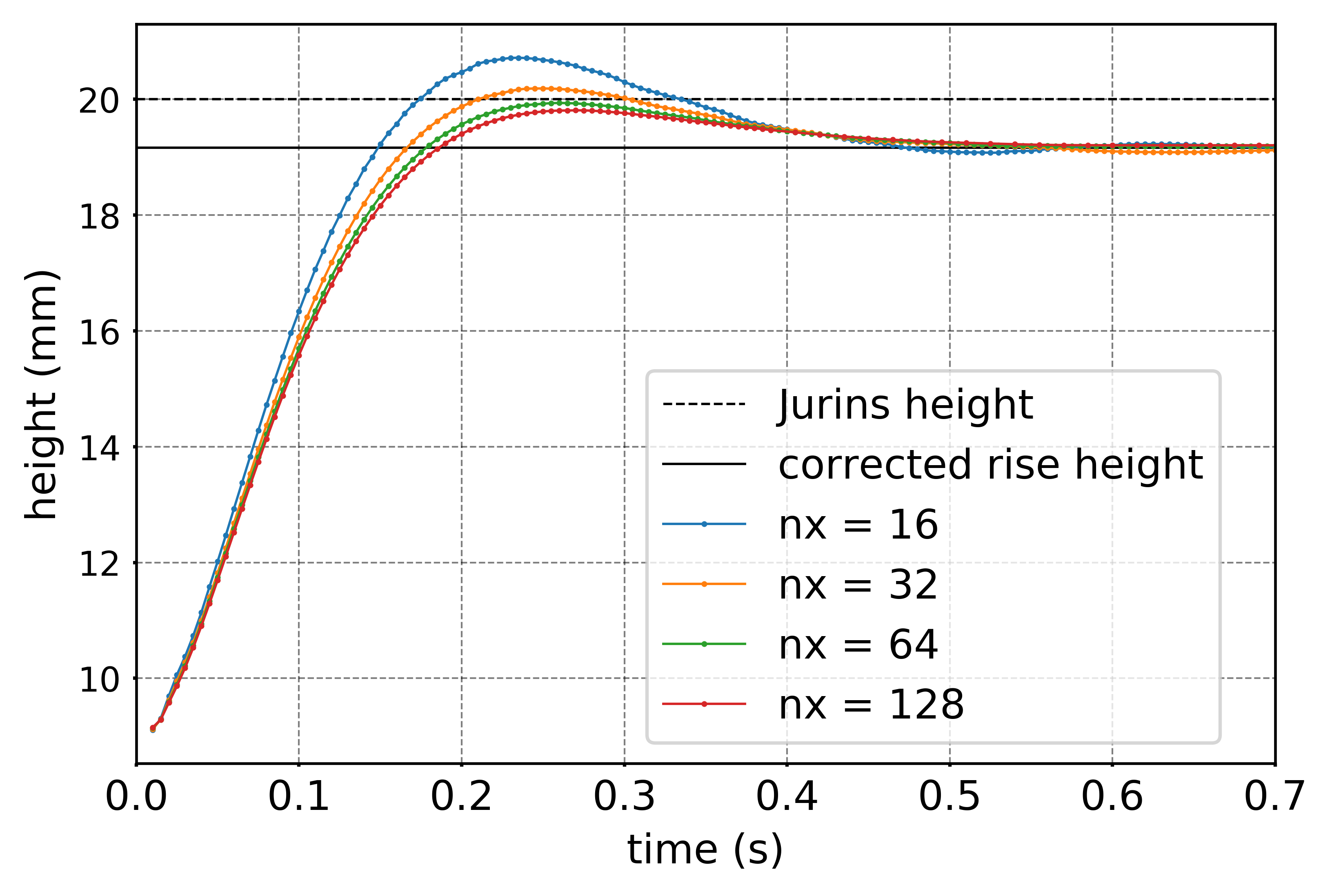
(b) Navier slip with slip length $\lambda=0.1\leavevmode\nobreak\ \mathrm{mm}$.

Figure 21: Mesh convergence study using a no-slip and a Navier slip boundary condition. Non-dimensionless number $\Omega=1$ and $\theta_{e}=30$°.

6.3 Effect of the dimensionless parameter $\Omega$ on the capillary rise

Figure 22 shows the simulation results for $\Omega=0.1$ and $\Omega=0.5$. A comparison of several other numerical methods with the plicRDF-isoAdvector method is also presented. As the $\Omega$ values chosen here are less than the critical value $\Omega_{c}=2$, we expect to see oscillations during the capillary rise from Bosanquet’s theory. The slip length is chosen to be $\lambda=R/5=1\leavevmode\nobreak\ \mathrm{mm}$. For $\Omega=0.1$ (see fig. 22(a)), we observe strong oscillations which decrease in amplitude with time and the solution asymptotically reaches the reference (corrected) rise height value. It can also be noted that for the first two peaks, the plicRDF-isoAdvector scheme’s result resembles the interFoam solver’s result. However, with time, the oscillations for the plicRDF-isoAdvector method are dampened slightly faster than with the other numerical methods. Similar behavior can be observed for $\Omega=0.5$ (see fig. 22(b)), but with fewer oscillations, and the simulations results level with the stationary height according to eq. 47.

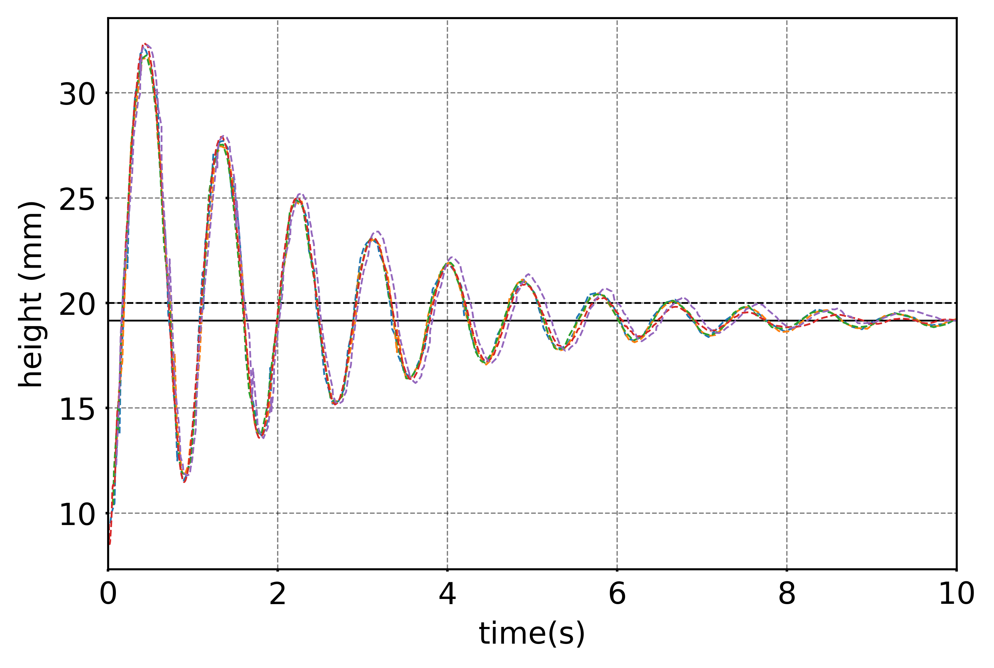
(a) $\Omega=0.1$.

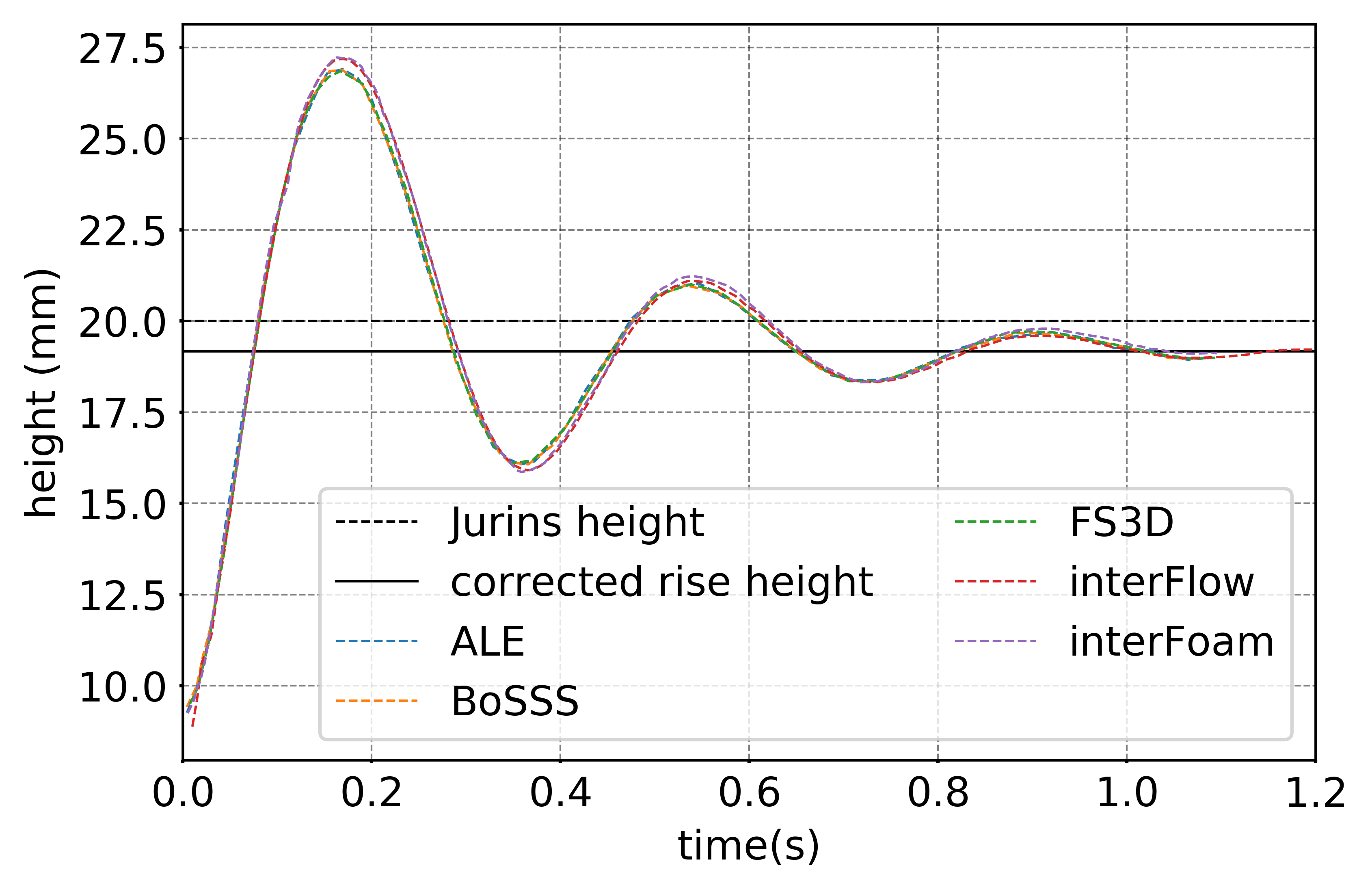
(b) $\Omega=0.5$.

Figure 22: Numerical result for capillary rise for the $\Omega$-study (oscillatory regime).

7 Conclusions and Outlook

We have benchmarked the plicRDF-isoAdvector method for wetting through four case studies. The first study investigated interface advection where a first- to second-order convergence transition is observed. The second study validated the contact line spreading dynamics on a flat surface with an excellent agreement to reference solutions, except for highly hydrophobic cases. The third study tested the method for droplet spreading on a spherical surface showing accurate results but with some sensitivity to numerical noise. The last study was a 2D capillary rise, with mesh-convergent results for the stationary state and contact line dynamics. The benchmark’s input data and post-processing Jupyter Notebooks are publicly available [25, 26] and provide a valuable starting point for benchmarking numerical methods for wetting processes.

The plicRDF-isoAdvector method can effectively simulate a broad spectrum of wetting problems. However, there are still challenges in simulating contact angles that are either very small (hydrophilic support) or very large (hydrophobic support). The plicRDF reconstruction indirectly considers the contact angle at the wall through a weighted sum of signed-distance values whose discrete gradient determines the cell-centered interface orientation. Also, the influence of the contact angle in the kinematic motion of a PLIC interface is mediated by the cell-centered PLIC interface orientation. Therefore, future developments should reconsider the approach via weighted contribution of the contact angle in the RDF PLIC reconstruction. From the gained experience, we recommend local adaptive mesh refinement near the interface with at least three cell layers of as uniform as possible mesh resolution surrounding the interface. Although plicRDF-isoAdvector can handle mesh grading, an interface passing through a non-uniform mesh-grading near a wall causes a loss in convergence order. An unstructured geometrical VOF interface reconstruction for contact line evolution is necessary, that exactly satisfies the prescribed contact angle in wall-adjacent cells, without this incurring a loss of accuracy away from wall-adjacent cell layer.

8 Acknowledgements

We acknowledge the financial support by the German Research Foundation (DFG) within the Collaborative Research Centre 1194 (Project-ID 265191195).

The use of the high-performance computing resources of the Lichtenberg High-Performance Cluster at the TU Darmstadt is gratefully acknowledged.

References

- Marengo and Coninck [2022] M. Marengo, J. D. Coninck (Eds.), The Surface Wettability Effect on Phase Change, Springer International Publishing, 2022. doi:10.1007/978-3-030-82992-6.
- Dhillon et al. [2015] N. S. Dhillon, J. Buongiorno, K. K. Varanasi, Critical heat flux maxima during boiling crisis on textured surfaces, Nature Communications 6 (2015). doi:10.1038/ncomms9247.
- Marić et al. [2020] T. Marić, D. B. Kothe, D. Bothe, Unstructured un-split geometrical Volume-of-Fluid methods – A review, Journal of Computational Physics 420 (2020) 109695. doi:https://doi.org/10.1016/j.jcp.2020.109695.
- Gibou et al. [2018] F. Gibou, R. Fedkiw, S. Osher, A review of level-set methods and some recent applications, Journal of Computational Physics 353 (2018) 82–109. doi:https://doi.org/10.1016/j.jcp.2017.10.006.
- Saye and Sethian [2020] R. I. Saye, J. A. Sethian, A review of level set methods to model interfaces moving under complex physics: Recent challenges and advances, in: Handbook of Numerical Analysis, volume 21, Elsevier, 2020. doi:10.1016/bs.hna.2019.07.003.
- OpenCFD Ltd. [2006] OpenCFD Ltd., OpenFOAM: user Guide v2006, 2006. https://openfoam.com/documentation/guides/latest/doc/, Last accessed on 2020-10-12.
- Deshpande et al. [2012] S. S. Deshpande, L. Anumolu, M. F. Trujillo, Evaluating the performance of the two-phase flow solver interFoam, Computational science & discovery 5 (2012) 014016. doi:10.1088/1749-4699/5/1/014016.
- Roenby et al. [2016] J. Roenby, H. Bredmose, H. Jasak, A computational method for sharp interface advection, Royal Society open science 3 (2016) 160405. doi:https://doi.org/10.1098/rsos.160405.
- Scheufler and Roenby [2019] H. Scheufler, J. Roenby, Accurate and efficient surface reconstruction from volume fraction data on general meshes, Journal of Computational Physics 383 (2019) 1–23. doi:https://doi.org/10.1016/j.jcp.2019.01.009.
- Gamet et al. [2020] L. Gamet, M. Scala, J. Roenby, H. Scheufler, J.-L. Pierson, Validation of volume-of-fluid OpenFOAM® isoAdvector solvers using single bubble benchmarks, Computers & Fluids 213 (2020) 104722. doi:https://doi.org/10.1016/j.compfluid.2020.104722.
- Popinet [2015] S. Popinet, A quadtree-adaptive multigrid solver for the Serre–Green–Naghdi equations, Journal of Computational Physics 302 (2015) 336–358. doi:https://doi.org/10.1016/j.jcp.2015.09.009.
- Osher and Sethian [1988] S. Osher, J. A. Sethian, Fronts propagating with curvature-dependent speed: Algorithms based on Hamilton-Jacobi formulations, Journal of Computational Physics 79 (1988) 12–49. doi:https://doi.org/10.1016/0021-9991(88)90002-2.
- Turek [1999] S. Turek, Efficient Solvers for Incompressible Flow Problems: An Algorithmic and Computational Approache, volume 6, Springer Science & Business Media, 1999.
- Parolini and Burman [2005] N. Parolini, E. Burman, A finite element level set method for viscous free-surface flows, in: Applied and industrial mathematics in Italy, World Scientific, 2005, pp. 416–427. doi:https://doi.org/10.1142/9789812701817_0038.
- John and Matthies [2004] V. John, G. Matthies, MooNMD–a program package based on mapped finite element methods, Computing and Visualization in Science 6 (2004) 163–170. doi:https://doi.org/10.1007/s00791-003-0120-1.
- Siriano et al. [2022] S. Siriano, N. Balcázar, A. Tassone, J. Rigola, G. Caruso, Numerical Simulation of High-Density Ratio Bubble Motion with interIsoFoam, Fluids 7 (2022) 152. doi:https://doi.org/10.3390/fluids7050152.
- Fricke et al. [2020] M. Fricke, T. Marić, D. Bothe, Contact line advection using the geometrical Volume-of-Fluid method, Journal of Computational Physics 407 (2020) 109221. doi:https://doi.org/10.1016/j.jcp.2019.109221.
- Dupont and Legendre [2010] J.-B. Dupont, D. Legendre, Numerical simulation of static and sliding drop with contact angle hysteresis, Journal of Computational Physics 229 (2010) 2453–2478. doi:https://doi.org/10.1016/j.jcp.2009.07.034.
- Fricke et al. [2020] M. Fricke, B. Fickel, M. Hartmann, D. Gründing, M. Biesalski, D. Bothe, A geometry-based model for spreading drops applied to drops on a silicon wafer and a swellable polymer brush film, arXiv preprint arXiv:2003.04914 (2020). doi:10.48550/ARXIV.2003.04914.
- Patel et al. [2017] H. Patel, S. Das, J. Kuipers, J. Padding, E. Peters, A coupled Volume of Fluid and Immersed Boundary Method for simulating 3D multiphase flows with contact line dynamics in complex geometries, Chemical Engineering Science 166 (2017) 28–41. doi:https://doi.org/10.1016/j.ces.2017.03.012.
- Gründing et al. [2020] D. Gründing, M. Smuda, T. Antritter, M. Fricke, D. Rettenmaier, F. Kummer, P. Stephan, H. Marschall, D. Bothe, A comparative study of transient capillary rise using direct numerical simulations, Applied Mathematical Modelling 86 (2020) 142–165. doi:https://doi.org/10.1016/j.apm.2020.04.020.
- Huh and Scriven [1971] C. Huh, L. E. Scriven, Hydrodynamic model of steady movement of a solid/liquid/fluid contact line, Journal of Colloid and Interface Science 35 (1971) 85–101. doi:https://doi.org/10.1016/0021-9797(71)90188-3.
- Quéré et al. [1999] D. Quéré, É. Raphaël, J.-Y. Ollitrault, Rebounds in a Capillary Tube, Langmuir 15 (1999) 3679–3682. doi:https://doi.org/10.1021/la9801615.
- Fries and Dreyer [2009] N. Fries, M. Dreyer, Dimensionless scaling methods for capillary rise, Journal of Colloid and Interface Science 338 (2009) 514–518. doi:https://doi.org/10.1016/j.jcis.2009.06.036.
- Asghar, M. H. and Marić, T. [2022] Asghar, M. H. and Marić, T. , plicRDF-isoAdvector benchmarks for wetting processes, 2022. https://github.com/CRC-1194/b01-wetting-benchmark, Last accessed on 2022-10-26.
- Asghar et al. [2022] M. H. Asghar, M. Fricke, D. Bothe, T. Marić, Validation and verification of the plicRDF-isoAdvector unstructured Volume-of-Fluid (VOF) method for wetting problems - parabolicFit curvature - input data, 2022. URL: https://tudatalib.ulb.tu-darmstadt.de/handle/tudatalib/3621. doi:10.48328/tudatalib-982.
- Kluyver et al. [2016] T. Kluyver, B. Ragan-Kelley, F. Pérez, B. Granger, M. Bussonnier, J. Frederic, K. Kelley, J. Hamrick, J. Grout, S. Corlay, P. Ivanov, D. Avila, S. Abdalla, C. Willing, J. development team, Jupyter Notebooks - a publishing format for reproducible computational workflows, in: F. Loizides, B. Scmidt (Eds.), Positioning and Power in Academic Publishing: Players, Agents and Agendas, IOS Press, Netherlands, 2016, pp. 87–90. URL: https://eprints.soton.ac.uk/403913/.
- Asghar et al. [2022] M. H. Asghar, M. Fricke, D. Bothe, T. Marić, Validation and verification of the plicRDF-isoAdvector unstructured Volume-of-Fluid (VOF) method for wetting problems - parabolicFit curvature - jupyter notebooks, csv files, secondary data, parameter variation file, 2022. URL: https://tudatalib.ulb.tu-darmstadt.de/handle/tudatalib/3622. doi:10.48328/tudatalib-983.
- OpenFOAM.com [2022] OpenFOAM.com, OpenFOAM-v2112, 2022. URL: https://develop.openfoam.com/Development/openfoam/-/tree/OpenFOAM-v2112.
- Scheufler [2022] H. Scheufler, TwoPhaseFlow, 2022. URL: https://github.com/DLR-RY/TwoPhaseFlow/tree/of2112.
- Bernhard Gschaider [2005] Bernhard Gschaider, Contrib/PyFoam, 2005. https://openfoamwiki.net/index.php/Contrib/PyFoam, Last accessed on 2020-10-19.
- Tolle et al. [2022] T. Tolle, D. Gründing, D. Bothe, T. Marić, triSurfaceImmersion: Computing volume fractions and signed distances from triangulated surfaces immersed in unstructured meshes, Computer Physics Communications 273 (2022) 108249. doi:https://doi.org/10.1016/j.cpc.2021.108249.
- Franjo Juretic [2021] Franjo Juretic, integration-cfmesh, 2021. https://develop.openfoam.com/Community/integration-cfmesh/-/commit/f362ee65334e08056abdabab45e588503553e0ef, build = 14aeaf8dab-20211220, Last accessed on 2022-10-19.
- Jürgen Riegel and van Havre [2022] W. M. Jürgen Riegel, Y. van Havre, freecad: A 3D parametric modeler, 2022. URL: https://www.freecadweb.org/.
- Youngs [1982] D. L. Youngs, Time-dependent multi-material flow with large fluid distortion, Numerical Methods for Fluid Dynamics (1982). URL: https://cir.nii.ac.jp/crid/1571417126191472512.
- Scardovelli and Zaleski [2003] R. Scardovelli, S. Zaleski, Interface reconstruction with least-square fit and split Eulerian–Lagrangian advection, International Journal for Numerical Methods in Fluids 41 (2003) 251–274. doi:https://doi.org/10.1002/fld.431.
- Cummins et al. [2005] S. J. Cummins, M. M. Francois, D. B. Kothe, Estimating curvature from volume fractions, Computers & Structures 83 (2005) 425–434. doi:https://doi.org/10.1016/j.compstruc.2004.08.017.
- Marić [2021] T. Marić, Iterative Volume-of-Fluid interface positioning in general polyhedrons with Consecutive Cubic Spline interpolation, Journal of Computational Physics: X 11 (2021) 100093. doi:https://doi.org/10.1016/j.jcpx.2021.100093.
- Tolle et al. [2020] T. Tolle, D. Bothe, T. Marić, SAAMPLE: A segregated accuracy-driven algorithm for multiphase pressure-linked equations, Computers & Fluids 200 (2020) 104450. doi:https://doi.org/10.1016/j.compfluid.2020.104450.
- Renardy et al. [2001] M. Renardy, Y. Renardy, J. Li, Numerical simulation of moving contact line problems using a volume-of-fluid method, Journal of Computational Physics 171 (2001) 243–263. doi:https://doi.org/10.1006/jcph.2001.6785.
- Scheufler and Roenby [2021] H. Scheufler, J. Roenby, TwoPhaseFlow: An OpenFOAM based framework for development of two phase flow solvers, arXiv preprint arXiv:2103.00870 (2021). doi:https://doi.org/10.48550/arXiv.2103.00870.
- Asghar et al. [2023a] M. H. Asghar, M. Fricke, D. Bothe, T. Marić, Numerical Wetting Benchmarks - Advancing the plicRDF-isoAdvector unstructured Volume-of-Fluid (VOF) method using the parabolic fit curvature model- Jupyter Notebooks, CSV files, Secondary Data, Parameter variation file, 2023a. URL: https://tudatalib.ulb.tu-darmstadt.de/handle/tudatalib/3622.5. doi:10.48328/tudatalib-983.5.
- Asghar et al. [2023b] M. H. Asghar, M. Fricke, D. Bothe, T. Marić, Numerical Wetting Benchmarks - Advancing the plicRDF-isoAdvector unstructured Volume-of-Fluid (VOF) method using the RDF curvature model- Jupyter Notebooks, CSV files, Secondary Data, Parameter variation file, 2023b. URL: https://tudatalib.ulb.tu-darmstadt.de/handle/tudatalib/3730.2. doi:10.48328/tudatalib-1069.2.
- Asghar et al. [2023c] M. H. Asghar, M. Fricke, D. Bothe, T. Marić, Numerical Wetting Benchmarks - Advancing the plicRDF-isoAdvector unstructured Volume-of-Fluid (VOF) method using height-function curvature model- Jupyter Notebooks, CSV files, Secondary Data, Parameter variation file, 2023c. URL: https://tudatalib.ulb.tu-darmstadt.de/handle/tudatalib/3729.2. doi:10.48328/tudatalib-1068.2.
- Fricke et al. [2019] M. Fricke, M. Köhne, D. Bothe, A kinematic evolution equation for the dynamic contact angle and some consequences, Physica D: Nonlinear Phenomena 394 (2019) 26–43. doi:https://doi.org/10.1016/j.physd.2019.01.008.
- Fricke et al. [2018] M. Fricke, M. Köhne, D. Bothe, On the kinematics of contact line motion, PAMM 18 (2018) e201800451. doi:https://doi.org/10.1002/pamm.201800451.
- Afkhami et al. [2009] S. Afkhami, S. Zaleski, M. Bussmann, A mesh-dependent model for applying dynamic contact angles to VOF simulations, Journal of Computational Physics 228 (2009) 5370–5389. doi:https://doi.org/10.1016/j.jcp.2009.04.027.
- Khatavkar et al. [2007] V. Khatavkar, P. Anderson, H. Meijer, Capillary spreading of a droplet in the partially wetting regime using a diffuse-interface model, Journal of Fluid Mechanics 572 (2007) 367–387. doi:https://doi.org/10.1017/S0022112006003533.
- Villanueva and Amberg [2006] W. Villanueva, G. Amberg, Some generic capillary-driven flows, International Journal of Multiphase Flow 32 (2006) 1072–1086. doi:https://doi.org/10.1016/j.ijmultiphaseflow.2006.05.003.
- Kitware, Inc, Los Alamos National Laboratory [2021] Kitware, Inc, Los Alamos National Laboratory , ParaView-v5.9, 2021. https://www.paraview.org/documentation/, Last accessed on 2022-10-19.
- Marić et al. [2018] T. Marić, H. Marschall, D. Bothe, An enhanced un-split face-vertex flux-based VoF method, Journal of Computational Physics 371 (2018) 967–993. doi:https://doi.org/10.1016/j.jcp.2018.03.048.
- Washburn [1921] E. W. Washburn, The Dynamics of Capillary Flow, Physical Review 17 (1921) 273–283. doi:10.1103/PhysRev.17.273.
- Bosanquet [1923] C. H. Bosanquet, On the flow of liquids into capillary tubes, The London, Edinburgh, and Dublin Philosophical Magazine and Journal of Science 45 (1923) 525–531. doi:https://doi.org/10.1080/14786442308634144.
- Gründing [2020] D. Gründing, An enhanced model for the capillary rise problem, International Journal of Multiphase Flow 128 (2020) 103210. doi:https://doi.org/10.1016/j.ijmultiphaseflow.2020.103210.
- Huh and Mason [1977] C. Huh, S. G. Mason, The steady movement of a liquid meniscus in a capillary tube, Journal of Fluid Mechanics 81 (1977) 401–419. doi:https://doi.org/10.1017/S0022112077002134.