Trust, but Verify: Using Self-Supervised Probing to Improve Trustworthiness

Abstract

Trustworthy machine learning is of primary importance to the practical deployment of deep learning models. While state-of-the-art models achieve astonishingly good performance in terms of accuracy, recent literature reveals that their predictive confidence scores unfortunately cannot be trusted: e.g., they are often overconfident when wrong predictions are made, or so even for obvious outliers. In this paper, we introduce a new approach of self-supervised probing, which enables us to check and mitigate the overconfidence issue for a trained model, thereby improving its trustworthiness. We provide a simple yet effective framework, which can be flexibly applied to existing trustworthiness-related methods in a plug-and-play manner. Extensive experiments on three trustworthiness-related tasks (misclassification detection, calibration and out-of-distribution detection) across various benchmarks verify the effectiveness of our proposed probing framework.

1 Introduction

Deep neural networks have recently exhibited remarkable performance across a broad spectrum of applications, including image classification and object detection. However, the ever-growing range of applications of neural networks has also led to increasing concern about the reliability and trustworthiness of their decisions [32, 17], especially in safety-critical domains such as autonomous driving and medical diagnosis. This concern has been exacerbated with observations about their overconfidence, where a classifier tends to give a wrong prediction with high confidence [27, 18]. Such disturbing phenomena are also observed on out-of-distribution data [16]. The overconfidence issue thus poses great challenges to the application of models in the tasks of misclassification detection, calibration and out-of-distribution detection [18, 14, 16], which we collectively refer to as trustworthiness.

Researchers have since endeavored to mitigate this overconfidence issue by deploying new model architectures under the Bayesian framework so as to yield well-grounded uncertainty estimates [3, 22, 12]. However, these proposed frameworks usually incur accuracy drops and heavier computational overheads. Deep ensemble models [24, 6] obtain uncertainty estimates from multiple classifiers, but also suffer from heavy computational cost. Some recent works [21, 8] favor improving misclassification detection performance given a trained classifier. In particular, Trust Score [21] relies on the training data to estimate the test sample’s misclassification probability, while True Class Probability [8] uses an auxiliary deep model to predict the true class probability in the original softmax distribution. Like these methods, our approach is plug-and-play and does not compromise the performance of the classifier, or require retraining it. Our method is complementary to existing trustworthiness methods, as we introduce the use of probing as a new source of information that can be flexibly combined with trustworthiness methods.

Probing [2, 20] was proposed as a general tool for understanding deep models without influencing the original model. Specifically, probing is an analytic framework that uses the representations extracted from an original model to train another classifier (termed ‘probing classifier’) for a certain designed probing task to predict some properties of interest. The performance (e.g., accuracy) of the learned probing classifier can be used to evaluate or understand the original model. For example, one probing framework proposed in [20] evaluates the quality of sentence embeddings using the performance on the probing task of sentence-length or word-order prediction, while [2] uses probing to understand the dynamics of intermediate layers in a deep network.

Though probing has been utilized in natural language processing for linguistics understanding, the potential of probing in mitigating the overconfidence issue in deep visual classifiers remains unexplored. Intuitively, our proposed framework uses probing to ‘assess’ a classifier, so as to distinguish inputs where it can be trusted from those where it cannot, based on the results on the probing task. To achieve this goal, we need both 1) well-designed probing tasks, which should be different but highly related to the original classification task, and 2) a framework for how to use the probing results.

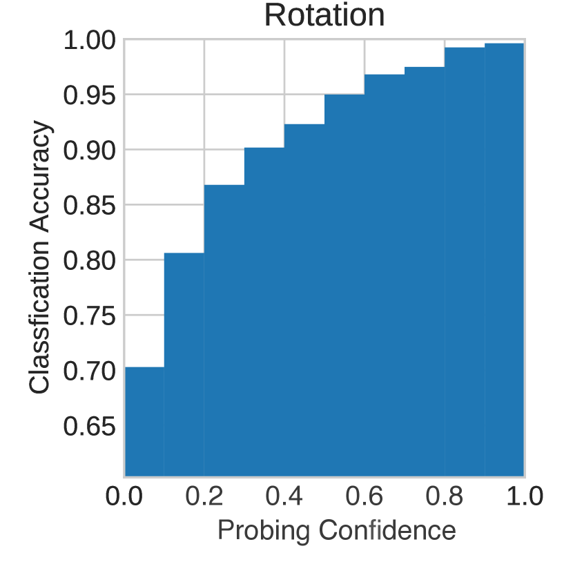
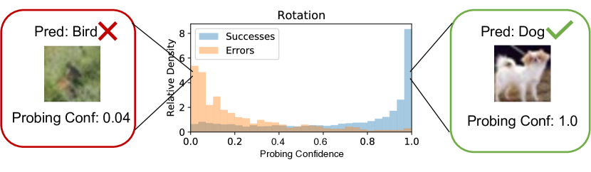
Figure 1: Left: Positive correlation between probing confidence and classification accuracy. Right: Images with lower probing confidence can be visually hard to detect and cause errors, while the images with higher probing confidences are sharp and clear, and lead to successful predictions. The visualized probing confidence is calculated from the self-supervised rotation task on CIFAR-10.

So the first question is: what probing tasks are related to the original visual classification problem yet naturally available and informative? We relate this question with the recent advancement of self-supervised learning. Existing literature suggests that a model that can tell the rotation, colorization or some other properties of objects is expected to have learned semantic information that is useful for downstream object classification [11, 28, 13, 36]. Reversing this, we may expect that a pretrained supervised model with good classification performance can tell the properties of an object, e.g., rotation degrees. In addition, recently [10] observes a strong correlation between rotation prediction accuracy and classification accuracy at the dataset level, under a multi-task learning scheme. This observation suggests that self-supervised tasks, e.g., rotation or translation prediction, can help in assessing a model’s trustworthiness.

In our work, we first present a novel empirical finding that the ‘probing confidence’, or the confidence of the probing classifier, highly correlates with the classification accuracy, as shown in Figure 1 and Figure 3. Motivated by this finding, we propose our self-supervised probing framework, which exploits the probing confidence for trustworthiness tasks, in a flexible and plug-and-play manner. Finally, we verify the effectiveness of our framework by conducting experiments on the three trustworthiness-related tasks.

Overall, the contributions and benefits of our approach are as follows:

• (Empirical Findings) We show that the probing confidence highly correlates with classification accuracy, showing the value of probing confidence as an auxiliary information source for trustworthiness tasks.

• (Generality) We provide a simple yet effective framework to incorporate the probing confidence into existing trustworthiness methods without changing the classifier architecture.

• (Effectiveness) We verify that our self-supervised probing framework achieves generally better performance in three trustworthiness related problems: misclassification detection, calibration and OOD detection.

2 Related Work

2.1 Trustworthiness in Deep Learning

The overconfidence issue [18, 16] raises major concerns about deep models’ trustworthiness, and has been studied in several related problems: calibration, misclassification detection, and out-of-distribution (OOD) detection [18, 14, 16].

Calibration algorithms aim to align a model’s predictive confidence scores with their ground truth accuracy. Among these methods, a prominent approach is to calibrate the confidence without changing the original prediction, such as Temperature Scaling [14] and Histogram Binning [4].

For misclassification and OOD detection, a common approach is to incorporate uncertainty estimation to get a well-grounded confidence score. For example, [25, 5] attempt to capture the uncertainty of every sample using a Dirichlet distribution. Ensemble-based methods such as Monte-Carlo Dropout [12] and Deep Ensembles [24] calculate uncertainty from multiple trials either with the Bayesian formalism or otherwise. However, these uncertainty estimation algorithms have a common drawback that they involve modifying the classification architecture, thus often incurring accuracy drops. Besides, ensembling multiple overconfident classifiers can still produce overconfident predictions.

The practical demand for uncertainty estimation on pretrained models has led to a line of research developing post-hoc methods. Trust Score [21] utilizes neighborhood information as a metric of trustworthiness, assuming that samples in a neighborhood are most likely to have the same class label. True Class Probability [8] aims to train a regressor to capture the softmax output score associated with the true class.

Compared to these works, we introduce probing confidence as a valuable additional source of information for trustworthiness tasks. Rather than replacing existing trustworthiness methods, our approach is complementary to them, flexibly incorporating them into our self-supervised probing framework.

2.2 Self-Supervised Learning

Self-supervised learning leverages supervisory signals from the data to capture the underlying structure of unlabeled data. Among them, a prominent paradigm [11, 28, 36] is to define a prediction problem for a certain property of interest (known as pretext tasks) and train a model to predict the property with the associated supervisory signals for representation learning. For example, some works train models to predict any given image’s rotation degree [13], or the relative position of image patches [28], or use multi-task learning combining supervised training with pretext tasks [19]. The core intuition behind these methods is that the proposed pretext tasks are highly related to the semantic properties in images. As such, well-trained models on these tasks are expected to have captured the semantic properties in images. Motivated by this intuition but from an opposite perspective, we expect that the supervised models that perform well in object classification, should have grasped the ability to predict relevant geometric properties of the data, such as rotation angle and translation offset.

2.3 Probing in Neural Networks

Early probing papers [23, 30] trained ‘probing classifiers’ on static word embeddings to predict various semantic properties. This analytic framework was then extended to higher-level embeddings, such as sentence embedding [1] and contextual embedding [31], by developing new probing tasks such as predicting the properties of the sentence structure (e.g., sentence length) or other semantic properties. Apart from natural language processing, probing has also been used in computer vision to investigate the dynamics of each intermediate layer in the neural network [2]. However, most probing frameworks are proposed as an explanatory tool for analyzing certain characteristics of learned representations or models. Instead, our framework uses the probing framework to mitigate the overconfidence issue, by using the probing results to distinguish samples on which the model is trustworthy, from samples on which it is not.

3 Methodology

3.1 Problem Formulation

Let us consider a dataset $\mathcal{D}$ which consists of $N$ i.i.d training samples, i.e., $\mathcal{D}={(\bm{\mathbf{x}}^{(i)},y^{(i)})}_{i=1}^{N}$ where $\bm{\mathbf{x}}^{(i)}\in\mathcal{R}^{d}$ is the $i$-th input sample and $y^{(i)}\in\mathcal{Y}=\{1,\ldots,K\}$ is the corresponding true class.

A classification neural network consists of two parts: the backbone parameterized by $\bm{\mathbf{\theta}}_{b}$ and the linear classification layer parameterized by $\bm{\mathbf{\theta}}_{c}$. Given an input $\mathbf{x}$, the neural network obtains a latent feature vector $\mathbf{z}=f_{\bm{\mathbf{\theta}}_{b}}(\mathbf{x})$ followed by the softmax probability output and the predictive label:

$$\hat{P}(Y\mid\mathbf{x},\bm{\mathbf{\theta}}_{b},\bm{\mathbf{\theta}}_{c})=\mathsf{softmax}(f_{\bm{\mathbf{\theta}}_{c}}(\mathbf{z}))$$ (1)

$$\hat{y}=\operatorname*{argmax}_{k\in\mathcal{Y}}\hat{P}(Y=k\mid\mathbf{x},\bm{\mathbf{\theta}}_{b},\bm{\mathbf{\theta}}_{c}).$$ (2)

The obtained maximum softmax probability (MSP) $\hat{p}\coloneqq\hat{P}(Y=\hat{y}\mid\mathbf{x},\bm{\mathbf{\theta}}_{b},\bm{\mathbf{\theta}}_{c})$ is broadly applied in the three trustworthiness tasks: misclassfication detection, out-of-distribution detection and calibration [18, 14].

3.1.1 Misclassification Detection

is also known as error or failure prediction [18, 8], and aims to predict whether a trained classifier makes an erroneous prediction for a test example. In general, it requires a confidence estimate for any given sample’s prediction, where a lower confidence indicates that the prediction is more likely to be wrong.

For a standard network, the baseline method is to use the maximum softmax output as the confidence estimate for misclassification detection [14, 18]:

$$\hat{P}(\hat{y}\neq y)\coloneqq 1-\hat{p}.$$ (3)

3.1.2 Out-Of-Distribution Detection

aims to detect whether a test sample is from a distribution that is different or semantically shifted from the training data distribution [34]. [18] proposed to use the maximum softmax scores for OOD detection. By considering the out-of-distribution data to come from a class that is not in $\mathcal{Y}$ (e.g. class $K+1$), we can write this as:

$$\hat{P}(y\in\mathcal{Y})\coloneqq\hat{p},$$ (4)

where $y$ is the true label for sample $\mathbf{x}$. The minimum value of this score is $1/K$, so an ideal classifier when given out-of-distribution data is expected to assign a flat softmax output probability of $1/K$ for each class [25].

3.1.3 Calibration

aims to align the predicted confidence $\hat{P}$ with the ground truth prediction accuracy. For example, with a well-calibrated model, samples predicted with confidence of $0.9$ should be correctly predicted $90\%$ of the time. Formally, we define perfect calibration as

$$\mathbb{P}(\hat{Y}=Y\mid\hat{P}=p)=p,\ \forall\ p\in[0,1],$$

where $\hat{P}$ is estimated as the maximum softmax probability in the standard supervised multi-class classification setup. However, these scores have commonly been observed to be miscalibrated, leading to a line of research into calibration techniques for neural networks, such as [14, 26].

On the whole, the baseline confidence scores (MSP) $\hat{p}$ have been observed to be often overconfident, even on misclassified as well as out-of-distribution samples [14, 18, 16]. This degrades the performance of the baseline approach on all three tasks: misclassification detection, OOD detection and calibration. Our work aims to show that self-supervised probing provides a valuable source of auxiliary information, which helps to mitigate the overconfidence issue and improve performance on these three tasks in a post-hoc setting.

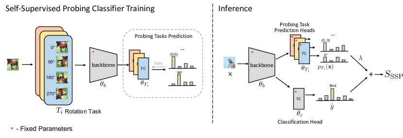
Figure 2: Our self-supervised probing framework, which first trains a probing classifier (left); then at test time, combines the probing confidence with the confidence obtained from the classifier.

3.2 Self-Supervised Probing Framework

3.2.1 Overview.

Our self-supervised probing framework computes the probing confidence, and uses it as an auxiliary source of information for the three trustworthiness tasks, given a trained classifier. Our framework involves two steps:

1. Training the self-supervised probing classifier to obtain the probing confidence for each sample;

2. Incorporating probing confidence into the three trustworthiness tasks. Specifically, for misclassification and OOD detection, we incorporate probing confidence by combining it with the original confidence scores. For calibration, we propose a simple and novel scheme which uses the probing confidence as prior information for input-dependent temperature scaling.

This framework is illustrated in Figure 2.

3.2.2 Self-Supervised Probing Tasks.

Recall that our goal is to use probing tasks to assess the trustworthiness of the classifier. This requires probing tasks that are semantically relevant to the downstream classification task (but without using the actual class labels). The observations made in [13, 36, 28]

suggest that simple tasks which apply a discrete set of transformations (e.g. a set of rotations or translations), and then require the model to predict which transformation was applied, should be suitable as probing tasks.

Formally, we denote the set of probing tasks as $\mathcal{T}=\{T_{1},T_{2},\ldots,T_{M}\}$, where each task $T_{i}$ consists of $k_{i}$ transformations $T_{i}=\{t_{i}^{(0)},t_{i}^{(1)},\ldots,t_{i}^{(k_{i}-1)}\}$, where $t_{i}^{(0)}$ is the identity transformation. For example, one can create a rotation probing task defined by four rotation transformations associated with rotation degrees of $\{0\degree,90\degree,180\degree,270\degree\}$, respectively.

3.2.3 Training Probing Classifier.

As our goal is to provide auxiliary uncertainty support for a given model, we avoid modifying or fine-tuning the original model and fix the model’s backbone throughout training. Thus, for a given probing task $T_{i}\in\mathcal{T}$, we fix the supervised model’s backbone $f_{\bm{\mathbf{\theta}}_{b}}$ and train the probing classifier as a fully-connected (FC) layer with parameters $\bm{\mathbf{\theta}}_{T_{i}}$. Optimization proceeds by minimizing the cross entropy loss $\mathcal{L}_{\text{CE}}$ over $\bm{\mathbf{\theta}}_{T_{i}}$ only:

$$\hat{P}(Y_{T_{i}} \mid t(\mathbf{x}),\bm{\mathbf{\theta}}_{b},\bm{\mathbf{\theta}}_{T_{i}}):=\mathsf{softmax}(f_{\bm{\mathbf{\theta}}_{T_{i}}}(f_{\bm{\mathbf{\theta}}_{b}}(t(\mathbf{x})))$$ (5)

$$\min_{\bm{\mathbf{\theta}}_{T_{i}}}\mathcal{L}_{T_{i}} :=\mathbb{E}_{(\mathbf{x},y)\sim\mathcal{D}}\sum_{t\in T_{i}}\mathcal{L}_{\text{CE}}(\mathbf{y}_{T_{i}},\hat{P}(Y_{T_{i}}\mid t(\mathbf{x}),\bm{\mathbf{\theta}}_{b},\bm{\mathbf{\theta}}_{T_{i}})),$$ (6)

where $\mathbf{y}_{T_{i}}$ is the one hot label for the probing task and $\mathcal{L}_{\text{CE}}$ denotes the cross entropy loss.

As the backbone is fixed for all probing tasks and there are no other shared parameters among probing tasks, the training for all probing tasks are performed in parallel. After training, we obtain $M$ probing classifiers for the probing tasks $\mathcal{T}$ ($|\mathcal{T}|=M$).

3.2.4 Computing Probing Confidence.

During inference, for each test image $\mathbf{x}$ and probing task $T_{i}$, we will now compute the probing confidence to help assess the model’s trustworthiness on $\mathbf{x}$. Intuitively, if the model is trustworthy on $\mathbf{x}$, the probing classifier should correctly recognize that $\mathbf{x}$ corresponds to an identity transformation (since it is the original untransformed test image). Thus, we probe the model by first passing the test image through the backbone, followed by applying the probing classifier corresponding to task $T_{i}$. Then, we compute the probing confidence $p_{T_{i}}(\mathbf{x})\in\mathbb{R}$ as the probing classifier’s predictive confidence for the identity transformation label (i.e. for label $0$) in the softmax probability distribution:

$$p_{T_{i}}(\mathbf{x}):=\hat{P}(\mathbf{y}_{T_{i}}^{(0)}\mid\mathbf{x},\bm{\mathbf{\theta}}_{b},\bm{\mathbf{\theta}}_{T_{i}})$$ (7)

3.2.5 Empirical Evidence.

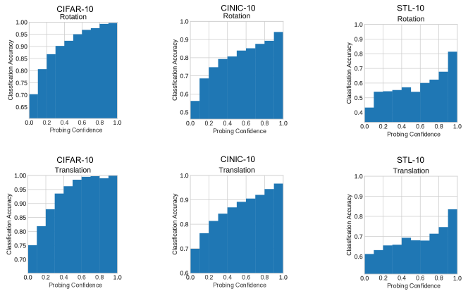
Figure 3: Clear positive correlation between classification accuracy and probing confidence under the rotation and translation probing tasks on CIFAR-10, CINIC-10 and STL-10.

From Figure 3, we observe that for both rotation and translation probing tasks, and on three datasets, the probing confidence has a clear positive correlation with the classification accuracy. This empirical evidence indicates that the samples with higher probing confidence tend to be predicted correctly in the classification task. This validates our use of probing confidence for assessing predictive confidence given a sample.

3.2.6 Incorporating Probing Confidence.

For the misclassification detection task, we compute our self-supervised probing score by combining the probing confidence from the different probing tasks with any existing misclassification score $S(\mathbf{x})$, which can be the classifier’s maximum softmax probability, entropy, or any other existing indicator scores [21, 8]:

$$S_{\text{SSP}}(\mathbf{x}):=S(\mathbf{x})+\sum_{i=1}^{M}\lambda_{i}p_{T_{i}}(\mathbf{x}),$$ (8)

where $\mathbf{\lambda}_{i}$’s are hyperparameters and are determined corresponding to the best AUPR-ERR performance on the validation set. The proposed $S_{\text{SSP}}(\mathbf{x})$ is the combined result from the original indicator and the probing confidence scores.

Similarly, we do the same for OOD detection, where $S(\mathbf{x})$ can be any existing OOD score, e.g. maximum softmax probability or entropy.

3.2.7 Input-Dependent Temperature Scaling.

For the calibration task, we design our input-dependent temperature scaling scheme to calibrate the original predictive confidence as an extension of temperature scaling [14]. Classical temperature scaling uses a single scalar temperature parameter $a_{0}$ to rescale the softmax distribution. Using our probing confidence $p_{T_{i}}(\mathbf{x})$ for each sample $\mathbf{x}$ as prior information, we propose to obtain a scalar temperature $\tau(\mathbf{x})$ as a learned function of the probing confidence:

$$\tau(\mathbf{x}) :=a_{0}+\sum_{i=1}^{M}a_{i}p_{T_{i}}(\mathbf{x})$$ (9)

$$\tilde{P}(Y\mid\mathbf{x}) :=\mathsf{softmax}\left(\frac{f_{\bm{\mathbf{\theta}}_{c}}\left(f_{\bm{\mathbf{\theta}}_{b}}(\mathbf{x})\right)}{\tau(\mathbf{x})}\right)$$ (10)

Here, $\tilde{P}(Y\mid\mathbf{x})$ contains our output calibrated probabilities. $a_{0}$ and $a_{i}$ are learnable parameters; they are optimized via negative likelihood loss on the validation set, similarly to in classical temperature scaling [14]. For each sample $\mathbf{x}$, we obtain $\tau(\mathbf{x})$ as its input-dependent temperature. With $\tau(\mathbf{x})=1$, we recover the original predicted probabilities $\hat{p}$ for the sample. As all logit outputs of a sample are divided by the same scalar, the predictive label is unchanged. In this way, we calibrate the softmax distribution based on the probing confidence, without compromising the model’s accuracy.

4 Experiments

In this section, we conduct experiments on the three trustworthiness-related tasks: misclassification, OOD detection and calibration. The main results including ablation study and case study focus on the misclassification detection task, while the experiments on calibration and OOD performance aim to verify the general effectiveness of probing confidence for trustworthiness-related tasks.

4.1 Experimental Setup

4.1.1 Datasets.

We conduct experiments on the benchmark image datasets: CIFAR-10 [33], CINIC-10 [9] and STL-10 [7]. We use the default validation split from CINIC-10 and split $20\%$ data from the labeled training data as validation set for CIFAR-10 and STL-10. All the models and baselines share the same setting. Further details about these datasets, architectures, training and evaluation metrics can be found in the supplementary material.

4.1.2 Network Architectures.

Our classification network architectures adopt the popular and effective models including VGG16 [29] and ResNet-18 [15]. For fairness, all methods share the same classification network. We train each probing task with a FC layer. The hyperparameters $\lambda_{i}$’s are selected according to the best AUPR-ERR performance on the corresponding validation set.

4.1.3 Evaluation Metrics.

The evaluation metrics for misclassification, OOD detection and calibration follow the standard metrics used in the literature [18, 8, 14]. We relegate the details to the supplementary material.

4.2 Results on Misclassification Detection

Table 1: Comparison of misclassification detection methods. All methods share the same trained classification network. All values are percentages. +SSP indicates incorporating our self-supervised probing. Bold numbers are the superior results.

FPR@95% $\downarrow$ AUPR-ERR $\uparrow$ AUPR-SUCC $\uparrow$ AUROC $\uparrow$ Dataset Model Base/+SSP CIFAR-10 VGG16 MSP 50.50/48.87 46.21/46.98 99.13/99.16 91.41/91.53 MCDropout 50.25/49.37 46.64/47.23 99.15/99.17 91.46/91.58 TCP 45.74/45.61 47.70/47.93 99.16/99.19 91.85/91.88 TrustScore 47.87/45.61 46.50/47.65 98.99/99.16 90.47/91.68 CIFAR-10 ResNet-18 MSP 47.01/45.30 44.39/45.48 99.02/99.32 90.63/92.10 MCDropout 43.47/38.18 42.04/52.60 99.53/99.51 93.09/94.05 TCP 40.88/40.88 50.37 /50.36 99.48/99.48 93.74/93.73 TrustScore 31.62/30.77 59.57/60.12 99.46/99.47 94.29/94.38 CINIC-10 VGG16 MSP 67.23/66.49 53.21/54.40 96.67/96.11 86.33/85.53 MCDropout 64.74/64.62 54.02/54.76 94.41/96.19 84.85/86.45 TCP 67.80/65.95 53.19/54.27 96.57/96.58 86.51/86.62 TrustScore 68.36/65.65 51.83/53.66 96.19/96.46 85.25/86.01 CINIC-10 ResNet-18 MSP 62.57/62.48 53.18/53.29 97.73/97.57 88.39/88.04 MCDropout 59.32/58.21 52.55/57.20 98.23/98.23 89.50/90.16 TCP 59.66/58.95 55.08/55.27 97.87/97.89 89.07/89.17 TrustScore 62.26/60.08 53.06/54.53 97.64/97.73 88.07/88.50 STL-10 ResNet-18 MSP 77.12/76.67 58.81/59.19 89.59/89.81 78.99/79.35 MCDropout 74.09/73.86 60.49/61.01 92.20/91.33 81.55/81.59 TCP 79.19/79.07 54.72/54.94 85.18/85.59 74.79/75.17 TrustScore 72.48/71.99 61.36/62.10 90.60/90.81 80.57/80.95

4.2.1 Performance.

To demonstrate the effectiveness of our framework, we implemented the baseline methods including Maximum Softmax Probabilty [18], Monte-Carlo Dropout (MCDropout) [12], Trust Score [21] and True Class Probability (TCP) [8]. Our implementation is based on the publicly released code (implementation details can be found in supplementary materials). To show the effectiveness of probing confidence for these existing trustworthiness scores, we compare the performance of models with and without our self-supervised probing approach (refer to Eq. (8), where we use the existing baseline methods as $S(\mathbf{x})$).

The results are summarized in Table 1. From the table, we observe that our method outperforms baseline scores in most cases. This confirms that probing confidence is a helpful indicator for failure or success prediction, and improves the existing state-of-the-art methods in a simple but effective way.

4.2.2 Q1: When does self-supervised probing adjust the original decision to be more (or less) confident?

As our goal is to provide auxiliary evidence support for predictive confidence based on self-supervised probing tasks, we investigate what kinds of images are made more or less confident by the addition of the probing tasks.

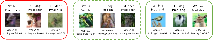
Figure 4: Analysis of the examples in CIFAR-10 for the rotation probing task. The red box contains the samples that are wrongly predicted on both probing and classification tasks. The green dashed box contains the samples predicted wrongly on the probing task but predicted correctly for classification. The green solid box contains the samples predicted correctly on both probing tasks and classification. The objects that are visually harder to detect tend to fail in the probing task.

Figure 4 illustrates three cases, demonstrating what kind of images tend to fail or succeed in the probing tasks. From the figure, we observe that samples with objects that are intrinsically hard to detect (e.g., hidden, blurred or blending in with their surroundings) tend to fail in the probing task, whereas samples with clear and sharp objects exhibit better performance in the probing task. The former type of samples are likely to be less trustworthy, which validates the intuition for our approach.

4.2.3 Q2: How do different combinations of probing tasks affect performance?

To further investigate the effect of the probing tasks, we design different combinations of probing tasks and observe how these combinations affect the performance in misclassification tasks.

We first demonstrate the performance with or without rotation and translation probing tasks to see how each task can affect the performance. The result is based on the ResNet-18 model trained on CIFAR-10 and reported in Table 2. The result shows that the rotation probing task contributes more than the translation task to the overall improvement. The combination of rotation and translation probing tasks outperforms each one individually, implying that multiple probing tasks better identifies the misclassified samples, by combining different perspectives.

Table 2: The performance of different combinations of probing tasks for CIFAR-10. Combining both probing tasks outperforms the individual task setting, suggesting that multiple tasks effectively assesses trustworthiness from multiple perspectives.

CIFAR-10 Rotation Translation FPR@95% $\downarrow$ AUPR-ERR $\uparrow$ AUPR-SUCC $\uparrow$ AUROC $\uparrow$ 45.30 45.48 99.32 92.10 45.58 45.36 99.28 91.78 46.15 44.61 99.24 91.42

To further investigate the influence of the number of transformations for each probing task, we conduct experiments by varying the numbers of transformations in the probing task.

The details of the experimental setting are provided in the supplementary material and the result is shown in Figure 5.

We observe that the larger dataset (CINIC-10) shows stable performance under the probing tasks with varying number of transformations, but the smaller dataset (STL-10) shows a drop in performance when using the probing tasks with more transformations. As the number of transformations in a probing task can be regarded as the complexity of the probing task, this suggests that on smaller datasets, the probing tasks should be designed with fewer transformations to allow the probing classifier to effectively learn the probing task.

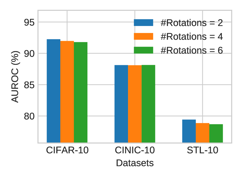
Figure 5: The performance (AUROC) when using different numbers of transformations (#Rotations / #Translations) in the rotation and translation probing tasks. The probing tasks with more transformations decrease the performance in most case, especially for the small dataset (STL-10).

4.2.4 Q3: Feasibility of other self-supervised tasks than rotation and translation prediction.

Other than rotation and translation, there are self-supervised tasks such as jigsaw puzzles [28], i.e., predicting the jigsaw puzzle permutations. Since our self-supervised probing framework can extract the probing confidence for any proposed self-supervised probing tasks flexibly, we also experiment with jigsaw puzzle prediction as a probing task. However, we found that the training accuracy for jigsaw puzzle prediction is low, resulting in less informative probing confidence scores. This is probably because shuffling patches of an image breaks down the image semantics, making it challenging for the supervised backbone to yield meaningful representations for the self-supervised probing task.

In general, probing tasks should be simple yet closely related to visual semantic properties, so that the probing confidence correlates with classification accuracy. The rotation and translation tasks assess a model’s ability to identify the correct orientation and position profile of the object of interest, which are closely related to the classification task; but more complex tasks (e.g., jigsaw) can lead to greater divergence between probing and classification. We leave the question of using other potential probing tasks in the further study.

4.3 Results on Out-of-Distribution Detection

Besides misclassification detection, we also conduct experiments on out-of-distribution detection with $S_{\text{SSP}}$. All hyperparameters $\lambda_{i}$ share the same setting as in misclassification detection. Since our goal is to verify that our self-supervised probing approach can be combined with common existing methods to enhance their performance, we build upon the most commonly used methods for OOD detection: Maximum Softmax Probability (MSP) and the entropy of the softmax probability distribution (refer to Eq. (8)).

The results are reported with the AUROC metric in Table 3, indicating that our self-supervised probing consistently improves the OOD detection performance on both MSP and entropy methods.

Table 3: AUROC (%) of OOD detection trained on in-distribution data (a) CIFAR-10 and (b) CINIC-10. The baseline methods are Maximum Softmax Probability and Entropy. +SSP indicates incorporating our self-supervised probing.

CIFAR-10 $\to$ Backbone Method SVHN LSUN ImageNet LSUN(FIX) ImageNet(FIX) VGG16 MSP 91.05 88.98 88.08 85.64 86.01 MSP+SSP 92.57 90.39 90.08 86.93 87.41 Entropy 91.79 89.55 88.60 86.04 86.46 Entropy+SSP 92.57 90.70 90.09 86.76 87.34 ResNet-18 MSP 88.80 91.17 88.86 85.26 85.75 MSP+SSP 91.71 92.62 91.27 89.71 89.65 Entropy 89.27 91.94 89.44 85.54 86.06 Entropy+SSP 92.13 93.55 92.02 90.04 90.03

CINIC-10 $\to$ Backbone Method SVHN LSUN ImageNet LSUN(FIX) ImageNet(FIX) VGG16 MSP 81.48 81.17 80.36 76.45 76.76 MSP+SSP 85.25 84.73 83.53 80.92 80.36 Entropy 83.24 82.96 81.92 77.83 77.93 Entropy+SSP 85.07 84.57 83.32 79.90 79.68 ResNet-18 MSP 88.81 86.11 83.03 83.25 81.59 MSP+SSP 90.33 87.87 86.20 83.69 83.43 Entropy 87.65 83.34 80.96 83.59 81.34 Entropy+SSP 89.75 85.46 83.26 85.09 83.31

4.4 Results on Calibration

In this section, we verify our proposed input-dependent temperature scaling as described in Section 3.2.7. Specifically, we compare the common calibration baselines, including Temperature Scaling [14] and Histogram Binning [35]. Temperature Scaling is the key baseline for verifying the effectiveness of our use of probing confidence as prior information to obtain a temperature for each sample.

The result is shown in Table 4. We observe that our proposed calibration method generally outperforms the baseline methods under different evaluation metrics.

Table 4: The reported performance in calibration. Our approach (Scaling+SSP) compare with uncalibrated softmax probability (MSP) [18], Histogram Binning binning (Hist. Binning) [35] and Temperature Scaling (Temp. Scaling) [14].

ECE (%) $\downarrow$ MCE (%) $\downarrow$ NLL $\downarrow$ Brier Score ($\times 10^{-3}$) $\downarrow$ CIFAR-10 VGG16 MSP (uncalibrated) 5.0 31.43 0.39 13.17 Hist. Binning 1.65 20.68 0.35 12.88 Temp. Scaling 1.03 7.53 0.26 12.03 Scaling+SSP 0.93 9.15 0.26 12.03 CIFAR-10 ResNet-18 MSP (uncalibrated) 4.31 28.16 0.28 11.55 Hist. Binning 1.17 27.95 0.31 10.73 Temp. Scaling 1.40 18.91 0.23 10.72 Scaling+SSP 0.75 7.92 0.22 10.48 CINIC-10 VGG16 MSP (uncalibrated) 9.68 24.29 0.71 27.82 Hist. Binning 2.95 28.40 0.67 26.44 Temp. Scaling 0.62 2.46 0.55 25.34 Scaling+SSP 0.53 3.42 0.55 25.28 CINIC-10 ResNet-18 MSP (uncalibrated) 7.94 23.08 0.55 23.43 Hist. Binning 2.26 21.09 0.56 22.20 Temp. Scaling 1.41 13.30 0.45 21.56 Scaling+SSP 0.77 10.22 0.44 21.51 STL-10 ResNet-18 MSP (uncalibrated) 16.22 26.76 1.18 46.73 Hist. Binning 7.80 17.73 1.92 46.30 Temp. Scaling 1.56 9.08 0.89 42.22 Scaling+SSP 1.17 7.61 0.89 42.15

5 Conclusions

In this paper, we proposed a novel self-supervised probing framework for enhancing existing methods’ performance on trustworthiness related problems. We first showed that the ‘probing confidence’ from the probing classifier highly correlates with classification accuracy. Motivated by this, our framework enables incorporating probing confidence into three trustworthiness related tasks: misclassification, OOD detection and calibration. We experimentally verify the benefits of our framework on these tasks. Our work suggests that self-supervised probing serves as a valuable auxiliary information source for trustworthiness tasks across a wide range of settings, and can lead to the design of further new methods incorporating self-supervised probing (and more generally, probing) into these and other tasks, such as continual learning and open-world settings.

Acknowledgements.

This work was supported in part by NUS ODPRT Grant R252-000-A81-133.

References

- [1] Adi, Y., Kermany, E., Belinkov, Y., Lavi, O., Goldberg, Y.: Fine-grained analysis of sentence embeddings using auxiliary prediction tasks. arXiv preprint arXiv:1608.04207 (2016)
- [2] Alain, G., Bengio, Y.: Understanding intermediate layers using linear classifier probes. arXiv preprint arXiv:1610.01644 (2016)
- [3] Blundell, C., Cornebise, J., Kavukcuoglu, K., Wierstra, D.: Weight uncertainty in neural networks. ArXiv abs/1505.05424 (2015)
- [4] Brier, G.W., et al.: Verification of forecasts expressed in terms of probability. Monthly weather review 78(1), 1–3 (1950)
- [5] Charpentier, B., Zügner, D., Günnemann, S.: Posterior network: Uncertainty estimation without ood samples via density-based pseudo-counts. Advances in Neural Information Processing Systems 33, 1356–1367 (2020)
- [6] Chen, J., Liu, F., Avci, B., Wu, X., Liang, Y., Jha, S.: Detecting errors and estimating accuracy on unlabeled data with self-training ensembles. Advances in Neural Information Processing Systems 34 (2021)
- [7] Coates, A., Ng, A., Lee, H.: An analysis of single-layer networks in unsupervised feature learning. In: Proceedings of the fourteenth international conference on artificial intelligence and statistics. pp. 215–223. JMLR Workshop and Conference Proceedings (2011)
- [8] Corbière, C., Thome, N., Bar-Hen, A., Cord, M., Pérez, P.: Addressing failure prediction by learning model confidence. arXiv preprint arXiv:1910.04851 (2019)
- [9] Darlow, L.N., Crowley, E.J., Antoniou, A., Storkey, A.J.: Cinic-10 is not imagenet or cifar-10. arXiv preprint arXiv:1810.03505 (2018)
- [10] Deng, W., Gould, S., Zheng, L.: What does rotation prediction tell us about classifier accuracy under varying testing environments? In: International Conference on Machine Learning. pp. 2579–2589. PMLR (2021)
- [11] Doersch, C., Gupta, A., Efros, A.A.: Unsupervised visual representation learning by context prediction. In: Proceedings of the IEEE international conference on computer vision. pp. 1422–1430 (2015)
- [12] Gal, Y., Ghahramani, Z.: Dropout as a bayesian approximation: Representing model uncertainty in deep learning. In: international conference on machine learning. pp. 1050–1059. PMLR (2016)
- [13] Gidaris, S., Singh, P., Komodakis, N.: Unsupervised representation learning by predicting image rotations. arXiv preprint arXiv:1803.07728 (2018)
- [14] Guo, C., Pleiss, G., Sun, Y., Weinberger, K.Q.: On calibration of modern neural networks. In: International Conference on Machine Learning. pp. 1321–1330. PMLR (2017)
- [15] He, K., Zhang, X., Ren, S., Sun, J.: Deep residual learning for image recognition. In: Proceedings of the IEEE conference on computer vision and pattern recognition. pp. 770–778 (2016)
- [16] Hein, M., Andriushchenko, M., Bitterwolf, J.: Why relu networks yield high-confidence predictions far away from the training data and how to mitigate the problem. In: Proceedings of the IEEE/CVF Conference on Computer Vision and Pattern Recognition. pp. 41–50 (2019)
- [17] Hendrycks, D., Carlini, N., Schulman, J., Steinhardt, J.: Unsolved problems in ml safety. arXiv preprint arXiv:2109.13916 (2021)
- [18] Hendrycks, D., Gimpel, K.: A baseline for detecting misclassified and out-of-distribution examples in neural networks. Proceedings of International Conference on Learning Representations (2017)
- [19] Hendrycks, D., Mazeika, M., Kadavath, S., Song, D.: Using self-supervised learning can improve model robustness and uncertainty. Advances in Neural Information Processing Systems 32 (2019)
- [20] Hewitt, J., Liang, P.: Designing and interpreting probes with control tasks. arXiv preprint arXiv:1909.03368 (2019)
- [21] Jiang, H., Kim, B., Guan, M.Y., Gupta, M.: To trust or not to trust a classifier. In: Proceedings of the 32nd International Conference on Neural Information Processing Systems. pp. 5546–5557 (2018)
- [22] Kendall, A., Gal, Y.: What uncertainties do we need in bayesian deep learning for computer vision? Advances in neural information processing systems 30 (2017)
- [23] Köhn, A.: What’s in an embedding? analyzing word embeddings through multilingual evaluation (2015)
- [24] Lakshminarayanan, B., Pritzel, A., Blundell, C.: Simple and scalable predictive uncertainty estimation using deep ensembles. Advances in Neural Information Processing Systems 30 (2017)
- [25] Malinin, A., Gales, M.: Predictive uncertainty estimation via prior networks. Advances in neural information processing systems 31 (2018)
- [26] Mukhoti, J., Kulharia, V., Sanyal, A., Golodetz, S., Torr, P.H.S., Dokania, P.: Calibrating deep neural networks using focal loss. ArXiv abs/2002.09437 (2020)
- [27] Nguyen, A., Yosinski, J., Clune, J.: Deep neural networks are easily fooled: High confidence predictions for unrecognizable images. In: Proceedings of the IEEE conference on computer vision and pattern recognition. pp. 427–436 (2015)
- [28] Noroozi, M., Favaro, P.: Unsupervised learning of visual representations by solving jigsaw puzzles. In: European conference on computer vision. pp. 69–84. Springer (2016)
- [29] Simonyan, K., Zisserman, A.: Very deep convolutional networks for large-scale image recognition. arXiv preprint arXiv:1409.1556 (2014)
- [30] Sohn, K., Lee, H., Yan, X.: Learning structured output representation using deep conditional generative models. Advances in neural information processing systems 28, 3483–3491 (2015)
- [31] Tenney, I., Xia, P., Chen, B., Wang, A., Poliak, A., McCoy, R.T., Kim, N., Van Durme, B., Bowman, S.R., Das, D., et al.: What do you learn from context? probing for sentence structure in contextualized word representations. arXiv preprint arXiv:1905.06316 (2019)
- [32] Toreini, E., Aitken, M., Coopamootoo, K., Elliott, K., Zelaya, C.G., Van Moorsel, A.: The relationship between trust in ai and trustworthy machine learning technologies. In: Proceedings of the 2020 conference on fairness, accountability, and transparency. pp. 272–283 (2020)
- [33] Torralba, A., Fergus, R., Freeman, W.T.: 80 million tiny images: A large data set for nonparametric object and scene recognition. IEEE transactions on pattern analysis and machine intelligence 30(11), 1958–1970 (2008)
- [34] Yang, J., Zhou, K., Li, Y., Liu, Z.: Generalized out-of-distribution detection: A survey. arXiv preprint arXiv:2110.11334 (2021)
- [35] Zadrozny, B., Elkan, C.: Obtaining calibrated probability estimates from decision trees and naive bayesian classifiers. In: Icml. vol. 1, pp. 609–616. Citeseer (2001)
- [36] Zhang, R., Isola, P., Efros, A.A.: Colorful image colorization. In: European conference on computer vision. pp. 649–666. Springer (2016)