Multi-Source Diffusion Models for
Simultaneous Music Generation and Separation

Abstract

In this work, we define a diffusion-based generative model capable of both music synthesis and source separation by learning the score of the joint probability density of sources sharing a context. Alongside the classic total inference tasks (i.e., generating a mixture, separating the sources), we also introduce and experiment on the partial generation task of source imputation, where we generate a subset of the sources given the others (e.g., play a piano track that goes well with the drums). Additionally, we introduce a novel inference method for the separation task based on Dirac likelihood functions. We train our model on Slakh2100, a standard dataset for musical source separation, provide qualitative results in the generation settings, and showcase competitive quantitative results in the source separation setting. Our method is the first example of a single model that can handle both generation and separation tasks, thus representing a step toward general audio models.

1 Introduction

Generative models have recently gained a lot of attention thanks to their successful application in many fields, such as NLP [43, 67], image synthesis [49, 50] or protein design [60]. The audio domain is no exception to this trend [1, 33].

A peculiarity of the audio domain is that an audio sample $\mathbf{y}$ can be seen as the sum of multiple individual source $\{\mathbf{x}_{1},\dots,\mathbf{x}_{N}\}$, resulting in a mixture $\mathbf{y}=\sum_{n=1}^{N}\mathbf{x}_{n}$. Unlike in other sub-fields of the audio domain (e.g., speech), sources present in musical mixtures (stems) share a context given their strong interdependence. For example, the bass line of a song follows the drum’s rhythm and harmonizes with the melody of the guitar. Mathematically, this fact can be expressed by saying that the joint distribution of the sources $p(\mathbf{x}_{1},\dots,\mathbf{x}_{N})$ does not factorize into the product of individual source distributions $\{p_{n}(\mathbf{x}_{n})\}_{n=1,\dots,N}$. Knowing the joint $p(\mathbf{x}_{1},\dots,\mathbf{x}_{N})$ implies knowing the distribution over the mixtures $p(\mathbf{y})$ since the latter can be obtained through the sum. The converse is more difficult mathematically, being an inverse problem.

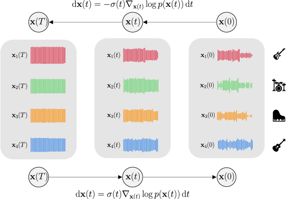
Figure 1: Diagram illustrating our proposed method. We leverage a forward Gaussian process (right-to-left) to learn the score over contextual sets (indicated by large rectangles) of instrumental sources (represented by waveforms) across different time steps $t$. During inference, the process is reversed (left-to-right), enabling us to perform tasks such as total generation, partial generation, or source separation (detailed in Figure 2).

Nevertheless, humans have developed the ability to process multiple sound sources simultaneously in terms of synthesis (i.e., musical composition or generation) and analysis (i.e., source separation). More specifically, humans can synthesize multiple sources $\{\mathbf{x}_{1},\dots,\mathbf{x}_{N}\}$ that sum to a coherent mixture $\mathbf{y}$ and extract the individual sources $\{\mathbf{x}_{1},\dots,\mathbf{x}_{N}\}$ from a mixture $\mathbf{y}$. This ability to compose and decompose sound is crucial for a generative music model. A model designed to assist in music composition should be capable of isolating individual sources within a mixture and allow for independent operation on each source. Such a capability would give the composer maximum control over what to modify and retain in a composition. Therefore, we argue that the task of compositional music generation is highly connected to the task of music source separation.

To the best of our knowledge, no model in deep learning literature can perform both tasks simultaneously. Models designed for the generation task directly learn the distribution $p(\mathbf{y})$ over mixtures, collapsing the information needed for the separation task. In this case, we have accurate mixture modeling but no information about the individual sources. It is worth noting that approaches that model the distribution of mixtures conditioning on textual data [58, 1] face the same limitations. Conversely, models for source separation [8] either target $p(\mathbf{x}_{1},\dots,\mathbf{x}_{N}\mid\mathbf{y}$), conditioning on the mixture, or learn a single model $p_{n}(\mathbf{x}_{n})$ for each source distribution (in a weakly-supervised manner) and condition on the mixture during inference [21, 46]. In both cases, generating mixtures is impossible. In the first case, the model inputs a mixture, which hinders the possibility of unconditional modeling, not having direct access to $p(\mathbf{x}_{1},\dots,\mathbf{x}_{N})$ (or equivalently to $p(\mathbf{y})$). In the second case, while we can accurately model each source independently, all essential information about their interdependence is lost, preventing the possibility of generating coherent mixtures.

Contribution. Our contribution is three-fold. (i) First, we bridge the gap between source separation and music generation by learning $p(\mathbf{x}_{1},\dots,\mathbf{x}_{N})$, the joint (prior) distribution of contextual sources (i.e., those belonging to the same song). For this purpose, we use the denoising score-matching framework to train a Multi-Source Diffusion Model (MSDM). We can perform both source separation and music generation during inference by training this single model. Specifically, generation is achieved by sampling from the prior, while separation is carried out by conditioning the prior on the mixture and then sampling from the resulting posterior distribution. (ii) This new formulation opens the doors to novel tasks in the generative domain, such as source imputation, where we create accompaniments by generating a subset of the sources given the others (e.g., play a piano track that goes well with the drums). (iii) Lastly, to obtain competitive results on source separation with respect to state-of-the-art discriminative models [39] on the Slakh2100 [40] dataset, we propose a new procedure for computing the posterior score based on Dirac delta functions, exploiting the functional relationship between the sources and the mixture.

2 Related Work

2.1 Generative Models for Audio

Deep generative models for audio, learn, directly or implicitly, the distribution of mixtures, represented in our notation by $p(\mathbf{y})$, possibly conditioning on additional data such as text. Various general-purpose generative models, such as autoregressive models, GANs [12], and diffusion models, have been adapted for use in the audio field.

Autoregressive models have a well-established presence in audio modeling [69]. Jukebox [9] proposed to model musical tracks with Scalable Transformers [70] on hierarchical discrete representations obtained through VQ-VAEs [68]. Furthermore, using a lyrics conditioner, this method generated tracks with vocals following the text. However, while Jukebox could model longer sequences in latent space, the audio output suffered from quantization artifacts. By incorporating residual quantization [76], newer latent autoregressive models [2, 31] can handle extended contexts and output more coherent and naturally sounding generations. State-of-the-art latent autoregressive models for music, such as MusicLM [1], can guide generation by conditioning on textual embeddings obtained via large-scale contrastive pre-training [38, 19]. MusicLM can also input a melody and condition on text for style transfer. A concurrent work, SingSong [11], introduces vocal-to-mixture accompaniment generation. Our accompaniment generation procedure differs from the latter since we perform generation at the stem level in a composable way, while the former outputs a single accompaniment mixture.

DiffWave [30] and WaveGrad [4] were the first diffusion (score) based generative models in audio, tackling speech synthesis. Many subsequent models followed these preliminary works, mainly conditioned to solve particular tasks such as speech enhancement [35, 59, 56, 54], audio upsampling [32, 75], MIDI-to-waveform [41, 15], or spectrogram-to-MIDI generation [5]. The first work in source-specific generation with diffusion models is CRASH [52]. [74, 44, 33] proposed text-conditioned diffusion models to generate general sounds, not focusing on restricted classes such as speech or music. Closer to our work, diffusion models targeting the musical domain are Riffusion [13] and Moûsai [58]. Riffusion fine-tunes Stable Diffusion [50], a large pre-trained text-conditioned vision diffusion model, over STFT magnitude spectrograms. Moûsai performs generation in a latent domain, resulting in context lengths that surpass the minute. Our score network follows the design of the U-Net proposed in Moûsai, albeit using the waveform data representation.

2.2 Audio Source Separation

Existing audio source separation models can be broadly classified into discriminative and generative. Discriminative source separators are deterministic parametric models that input the mixtures and systematically extract one or all sources, maximizing the likelihood of some underlying conditional distribution $p(\mathbf{x}_{1},\dots,\mathbf{x}_{N}\mid\mathbf{y})$. These models are typically trained with a regression loss [14] on the estimated signal represented as waveform [34, 36, 8], STFT [66, 6], or both [7]. On the other hand, generative source separation models learn a prior model for each source, thus targeting the distributions $\{p_{n}(\mathbf{x}_{n})\}_{n=1,\dots,N}$. The mixture is observed only during inference, where a likelihood function connects it to its constituent sources. The literature has explored different priors, such as GANs [65, 29, 42], normalizing flows [21, 77], and autoregressive models [22, 46].

The separation method closer to ours is the NCSN-BASIS algorithm [21]. This method was proposed for source separation in the image domain, performing Langevin Dynamics for separating the mixtures with an NCSN score-based model. It employs a Gaussian likelihood function during inference, which, as we demonstrate experimentally, is sub-optimal compared to our novel Dirac-based likelihood function. The main difference between our method with respect to other generative source separation methods (including NCSN-BASIS) is the modeling of the full joint distribution. As such, we can perform source separation and synthesize mixtures or subsets of stems with a single model.

Contextual information between sources is explicitly modeled in [39] and [47]. The first work models the relationship between sources by training an orderless NADE estimator, which predicts a subset of the sources while conditioning on the input mixture and the remaining sources. The subsequent study achieves universal source separation [25, 73] through adversarial training, utilizing a context-based discriminator to model the relationship between sources. Both methods are discriminative, as they are conditioned on the mixtures architecturally. The same architectural limitation is present in discriminative approaches for source separation that use diffusion-based [57, 37] or diffusion-inspired [45] methods. Our method sets itself apart as it proposes a model not constrained architecturally by a mixture conditioner, so we can also perform unconditional generation.

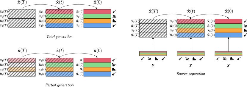
Figure 2: Inference tasks with MSDM. Oblique lines represent the presence of noise in the signal, decreasing from left to right, with the highest noise level at time $T$ when we start the sampling procedure. Top-left: We generate all stems in a mixture, obtaining a total generation. Bottom-left: We perform partial generation (source imputation) by fixing the sources $\mathbf{x}_{1}$ (Bass) and $\mathbf{x}_{3}$ (Piano) and generating the other two sources $\hat{\mathbf{x}}_{2}{(0)}$ (Drums) and $\hat{\mathbf{x}}_{4}{(0)}$ (Guitar). We denote with $\mathbf{x}_{1}(t)$ and $\mathbf{x}_{3}(t)$, the noisy stems obtained from $\mathbf{x}_{1}$ and $\mathbf{x}_{3}$ via the perturbation kernel in Eq. (1). Right: We perform source separation by conditioning the prior with a mixture $\mathbf{y}$, following Algorithm 1.

3 Background

The foundation of our model lies in estimating the joint distribution of the sources $p(\mathbf{x}_{1},\dots,\mathbf{x}_{N})$. Our approach is generative because we model an unconditional distribution (the prior). The different tasks are then solved at inference time, exploiting the prior.

We employ a diffusion-based [61, 17] generative model trained via denoising score-matching [63] to learn the prior. Specifically, we present our formalism by utilizing the framework established in [23]. The central idea of score-matching [20, 28, 72] is to approximate the “score” function of the target distribution $p(\mathbf{x})$, namely $\nabla_{\mathbf{x}}\log p(\mathbf{x})$, rather than the distribution itself. To effectively approximate the score in sparse data regions, denoising diffusion methods introduce controlled noise to the data and learn to remove it. Formally, the data distribution is perturbed with a Gaussian perturbation kernel:

$$p(\mathbf{x}(t)\mid\mathbf{x}(0))=\mathcal{N}(\mathbf{x}(t);\mathbf{x}(0),\sigma^{2}(t)\mathbf{I})\,,$$ (1)

where the parameter $\sigma(t)$ regulates the degree of noise added to the data. Following the authors in [23], we consider an optimal schedule given by $\sigma(t)=t$. With that choice of $\sigma(t)$, the forward evolution of a data point $\mathbf{x}(t)$ in time is described by a probability flow ODE[64]:

$$\mathrm{d}\mathbf{x}(t)=-\sigma(t)\nabla_{\mathbf{x}(t)}\log p(\mathbf{x}(t))\,\mathrm{d}t\,.$$ (2)

For $t=T>>0$, a data point $\mathbf{x}(T)$ is approximately distributed according to a Gaussian distribution $\mathcal{N}(\mathbf{x}(t);\mathbf{0},\sigma^{2}(T)\mathbf{I})$, from which sampling is straightforward. Eq. (2) can be inverted in time, resulting in the following backward ODE that describes the denoising process:

$$\mathrm{d}\mathbf{x}(t)=\sigma(t)\nabla_{\mathbf{x}(t)}\log p(\mathbf{x}(t))\,\mathrm{d}t\,.$$ (3)

Sampling can be performed from the data distribution integrating Eq. (3) with a standard ODE solver, starting from an initial (noisy) sample drawn from $\mathcal{N}(\mathbf{x}(t);\mathbf{0},\sigma^{2}(T)\mathbf{I})$. The score function, represented by a neural network $S^{\theta}(\mathbf{x}(t),\sigma(t))$, is approximated by minimizing the following score-matching loss:

$$\mathbb{E}_{t\sim\mathcal{U}([0,T])}\mathbb{E}_{\mathbf{x}(0)\sim p(\mathbf{x}(0))}\mathbb{E}_{\mathbf{x}(t)\sim p(\mathbf{x}(t)\mid\mathbf{x}(0))}\left\|S^{\theta}(\mathbf{x}(t),\sigma(t))-\nabla_{\mathbf{x}(t)}\log p\left(\mathbf{x}(t)\mid\mathbf{x}(0)\right)\right\|^{2}_{2}.$$

By expanding $p(\mathbf{x}(t)\mid\mathbf{x}(0))$ with Eq. (1), the score-matching loss simplifies to:

$$\mathbb{E}_{t\sim\mathcal{U}([0,T])}\mathbb{E}_{\mathbf{x}(0)\sim p(\mathbf{x}(0))}\mathbb{E}_{\mathbf{\epsilon}\sim\mathcal{N}(\mathbf{0},\sigma^{2}(t)\mathbf{I})}\left\|D^{\theta}(\mathbf{x}(0)+\mathbf{\epsilon},\sigma(t))-\mathbf{x}(0)\right\|_{2}^{2}\,,$$

where we define $S^{\theta}(\mathbf{x}(t),\sigma(t))=:(D^{\theta}(\mathbf{x}(t),\sigma(t))-\mathbf{x}(t))/\sigma^{2}(t)$.

4 Method

4.1 Multi-Source Audio Diffusion Models

In our setup, we have $N$ distinct source waveforms $\{\mathbf{x}_{1},\dots,\mathbf{x}_{N}\}$ with $\mathbf{x}_{n}\in\mathbb{R}^{D}$ for each $n$. The sources coherently sum to a mixture $\mathbf{y}=\sum_{n=1}^{N}\mathbf{x}_{n}$. We sometimes use the aggregated form $\mathbf{x}=(\mathbf{x}_{1},\dots,\mathbf{x}_{N})\in\mathbb{R}^{N\times D}$.

In this setting, multiple tasks can be performed: one may generate a consistent mixture $\mathbf{y}$ or separate the individual sources $\mathbf{x}$ from a given mixture $\mathbf{y}$. We refer to the first task as generation and the second as source separation. A subset of sources can also be fixed in the generation task, and the others can be generated consistently. We call this task partial generation or source imputation. Our key contribution is the ability to perform all these tasks simultaneously by training a single multi-source diffusion model (MSDM), capturing the prior $p(\mathbf{x}_{1},\dots,\mathbf{x}_{N})$. The model, illustrated in Figure 1, approximates the noisy score function:

$$\nabla_{\mathbf{x}(t)}\log p(\mathbf{x}(t))=\nabla_{(\mathbf{x}_{1}(t),\dots,\mathbf{x}_{N}(t))} \log p(\mathbf{x}_{1}(t),\dots,\mathbf{x}_{N}(t))\,,$$

with a neural network:

$$S^{\theta}(\mathbf{x}(t),\sigma(t)):\mathbb{R}^{N\times D}\times\mathbb{R}\rightarrow\mathbb{R}^{N\times D}\,,$$ (4)

where $\mathbf{x}(t)=(\mathbf{x}_{1}(t),\dots,\mathbf{x}_{N}(t))$ denotes the sources perturbed with the Gaussian kernel in Eq. (1). We describe the three tasks (illustrated in Figure 2) using the prior distribution:

• Total Generation. This task requires generating a plausible mixture $\mathbf{y}$. It can be achieved by sampling the sources $\{\mathbf{x}_{1},...,\mathbf{x}_{N}\}$ from the prior distribution and summing them to obtain the mixture $\mathbf{y}$.

• Partial Generation. Given a subset of sources, this task requires generating a plausible accompaniment. We define the subset of fixed sources as $\mathbf{x}_{\mathcal{I}}$ and generate the remaining sources $\mathbf{x}_{\mathcal{\overline{I}}}$ by sampling from the conditional distribution $p(\mathbf{x}_{\overline{\mathcal{I}}}\mid\mathbf{x}_{\mathcal{I}})$.

• Source Separation. Given a mixture $\mathbf{y}$, this task requires isolating the individual sources that compose it. It can be achieved by sampling from the posterior distribution $p(\mathbf{x}\mid\mathbf{y})$.

4.2 Inference

The three tasks of our method are solved during inference by discretizing the backward Eq. (3). Although different tasks require distinct score functions, they all originate directly from the prior score function in Eq. (4). We analyze each of these score functions in detail. For more details on the discretization method, refer to Section 5.3.

4.2.1 Total Generation

The total generation task is performed by sampling from Eq. (3) using the score function in Eq. (4). The mixture is then obtained by summing over all the generated sources.

4.2.2 Partial Generation

In the partial generation task, we fix a subset of source indices $\mathcal{I}\subset\{1,\dots,N\}$ and the relative sources $\mathbf{x}_{\mathcal{I}}:=\{\mathbf{x}_{n}\}_{n\in\mathcal{I}}$. The goal is to generate the remaining sources $\mathbf{x}_{\overline{\mathcal{I}}}:=\{\mathbf{x}_{n}\}_{n\in\overline{\mathcal{I}}}$ consistently, where ${\overline{\mathcal{I}}}=\{1,\dots,N\}-\mathcal{I}$. To do so, we estimate the gradient of the conditional distribution:

$$\nabla_{\mathbf{x}_{\overline{\mathcal{I}}}(t)}\log p(\mathbf{x}_{\overline{\mathcal{I}}}(t)\mid\mathbf{x}_{\mathcal{I}}(t)).$$ (5)

This falls into the setting of imputation or, as it is more widely known in the image domain, inpainting. We approach imputation using the method in [64]. The gradient in Eq. (5) is approximated as follows:

$$\nabla_{\mathbf{x}_{\overline{\mathcal{I}}}(t)}\log p([\mathbf{x}_{\overline{\mathcal{I}}}(t),\hat{\mathbf{x}}_{\mathcal{I}}(t)])\,,$$

where $\hat{\mathbf{x}}_{\mathcal{I}}$ is a sample from the forward process: $\hat{\mathbf{x}}_{\mathcal{I}}(t)\sim\mathcal{N}(\mathbf{x}_{\mathcal{I}}(t);\mathbf{x}_{\mathcal{I}}(0),\sigma(t)^{2}\mathbf{I})$. The square bracket operator denotes concatenation. Approximating the score function, we write:

$$\nabla_{\mathbf{x}_{\overline{\mathcal{I}}}(t)}\log p(\mathbf{x}_{\overline{\mathcal{I}}}(t)\mid\mathbf{x}_{\mathcal{I}}(t))\approx S^{\theta}_{\overline{\mathcal{I}}}([\mathbf{x}_{\overline{\mathcal{I}}}(t),\hat{\mathbf{x}}_{\mathcal{I}}(t)],\sigma(t))\,,$$

where $S^{\theta}_{\overline{\mathcal{I}}}$ denotes the entries of the score network corresponding to the sources indexed by $\overline{\mathcal{I}}$.

Algorithm 1 ‘MSDM Dirac’ sampler for source separation.

0:  $I$ number of discretization steps for the ODE, $R$ number of corrector steps, $\{\sigma_{i}\}_{i\in\{0,\dots,I\}}$ noise schedule, $S_{\text{churn}}$

1:  Initialize $\hat{\mathbf{x}}\sim\mathcal{N}(0,\sigma^{2}_{I}\mathbf{I})$

2:  $\alpha\leftarrow\min(S_{\text{churn}}/I,\sqrt{2}-1)$

3:  for $i\leftarrow I$ to $1$ do

4:     for $r\leftarrow R$ to $0$ do

5:        $\hat{\sigma}\leftarrow\sigma_{i}\cdot(\alpha+1)$

6:        $\mathbf{\epsilon}\sim\mathcal{N}(0,\mathbf{I})$

7:        $\hat{\mathbf{x}}\leftarrow\hat{\mathbf{x}}+\sqrt{\hat{\sigma}^{2}-\sigma_{i}^{2}}\mathbf{\epsilon}$

8:        $\mathbf{z}\leftarrow[\hat{\mathbf{x}}_{1:N-1},\mathbf{y}-\sum_{n=1}^{N-1}\hat{\mathbf{x}}_{n}]$

9:        for $n\leftarrow 1$ to $N-1$ do

10:           $\mathbf{g}_{n}\leftarrow S^{\theta}_{n}(\mathbf{z},\hat{\sigma})-S^{\theta}_{N}(\mathbf{z},\hat{\sigma})$

11:        end for

12:        $\mathbf{g}\leftarrow[\mathbf{g}_{1},\dots,\mathbf{g}_{N-1}]$

13:        $\hat{\mathbf{x}}_{1:N-1}\leftarrow\hat{\mathbf{x}}_{1:N-1}+(\sigma_{i-1}-\hat{\sigma})\mathbf{g}$

14:        $\hat{\mathbf{x}}\leftarrow[\hat{\mathbf{x}}_{1:N-1},\mathbf{y}-\sum_{n=1}^{N-1}\hat{\mathbf{x}}_{n}]$

15:        if $r>0$ then

16:           $\mathbf{\epsilon}\sim\mathcal{N}(0,\mathbf{I})$

17:           $\hat{\mathbf{x}}\leftarrow\hat{\mathbf{x}}+\sqrt{\sigma_{i}^{2}-\sigma_{i-1}^{2}}\mathbf{\epsilon}$

18:        end if

19:     end for

20:  end for

21:  return $\hat{\mathbf{x}}$

4.2.3 Source Separation

We view source separation as a specific instance of conditional generation, where we condition the generation process on the given mixture $\mathbf{y}=\mathbf{y}(0)$. This requires computing the score function of the posterior distribution:

$$\nabla_{\mathbf{x}(t)}\log p(\mathbf{x}(t)\mid\mathbf{y}(0))\,.$$ (6)

Standard methods for implementing conditional generation for diffusion models involve directly estimating the posterior score in Eq. (6) at training time (i.e., Classifier Free Guidance, as described in [18]) or estimating the likelihood function $p(\mathbf{y}(0)\mid\mathbf{x}(t))$ and using the Bayes formula to derive the posterior. The second approach typically involves training a separate model, often a classifier, for the score of the likelihood function as in Classifier Guided conditioning, outlined in [10].

In diffusion-based generative source separation, learning a likelihood model is typically unnecessary because the relationship between $\mathbf{x}(t)$ and $\mathbf{y}(t)$ is represented by a simple function, namely the sum. A natural approach is to model the likelihood function based on such functional dependency. This is the approach taken by [21], where they use a Gaussian likelihood function:

$$p(\mathbf{y}(t)\mid\mathbf{x}(t))=\mathcal{N}(\mathbf{y}(t)\mid\sum_{n=1}^{N}\mathbf{x}_{n}(t),\gamma^{2}(t)\mathbf{I}),$$ (7)

with the standard deviation given by a hyperparameter $\gamma(t)$. The authors argue that aligning the $\gamma(t)$ value to be proportionate to $\sigma(t)$ optimizes the outcomes of their NCSN-BASIS separator.

We present a novel approximation of the posterior score function in Eq. (6) by modeling $p(\mathbf{y}(t)\mid\mathbf{x}(t))$ as a Dirac delta function centered in $\sum_{n=1}^{N}\mathbf{x}_{n}(t)$:

$$p(\mathbf{y}(t)\mid\mathbf{x}(t))=\mathbbm{1}_{\mathbf{y}(t)=\sum_{n=1}^{N}\mathbf{x}_{n}(t)}\,.$$ (8)

The complete derivation can be found in Appendix A, and we present only the final formulation, which we call ‘MSDM Dirac’. The method constrains a source, without loss of generality $\mathbf{x}_{N}$, by setting $\mathbf{x}_{N}(t)=\mathbf{y}(0)-\sum_{n=1}^{N-1}\mathbf{x}_{n}(t)$ and estimates:

$$\vspace{-1cm}\nabla_{\mathbf{x}_{m}(t)}\log p(\mathbf{x}(t)\mid\mathbf{y}(0)) \approx S^{\theta}_{m}((\mathbf{x}_{1}(t),\dots,\mathbf{x}_{N-1}(t),\mathbf{y}(0)-\sum_{n=1}^{N-1}\mathbf{x}_{n}(t)),\sigma(t))$$

$$-S^{\theta}_{N}((\mathbf{x}_{1}(t),\dots,\mathbf{x}_{N-1}(t),\mathbf{y}(0)-\sum_{n=1}^{N-1}\mathbf{x}_{n}(t)),\sigma(t))\,,\vspace{-1cm}$$

where $1\leq m\leq N-1$ and $S_{m}^{\theta},S_{N}^{\theta}$ denote the entries of the score network corresponding to the $m$-th and $N$-th sources. Our approach models the limiting case wherein $\gamma(t)\to 0$ in the Gaussian likelihood function. This represents a scenario where the functional dependence between $\mathbf{x}(t)$ and $\mathbf{y}(t)$ becomes increasingly tight, thereby sharpening the conditioning on the given mixture during the generation process. The pseudo-code for the ‘MSDM Dirac’ source separation sampler, using the Euler ODE integrator of [23], is provided in Algorithm 1. The Euler ODE discretization logic uses the $S_{\text{churn}}$ mechanism of [23] and optional correction steps [64] (see Section 5.3 for more details).

The separation procedure can be additionally employed in the weakly-supervised source separation scenario, typically encountered in generative source separation [21, 77, 46]. This scenario pertains to cases where we know that specific audio data belongs to a particular instrument class, but we do not have access to sets of sources that share a context. To adapt to this scenario, we assume independence between sources $p(\mathbf{x}_{1},\dots,\mathbf{x}_{N})=\prod_{n=1}^{N}p_{n}(\mathbf{x}_{n})$ and train a separate model for each source class. We call the resulting model ‘Weakly MSDM Dirac’. We derive its formula and formulas for the Gaussian likelihood versions ‘MSDM Gaussian’ and ‘Weakly MSDM Gaussian’ in Appendix B.

5 Experimental Setup

5.1 Dataset

We perform experiments on Slakh2100 [40], a standard dataset for music source separation. Slakh2100 is a collection of multi-track waveform music data synthesized from MIDI files using virtual instruments of professional quality. The dataset comprises 2100 tracks, with a distribution of 1500 tracks for training, 375 for validation, and 225 for testing. Each track is accompanied by its stems, which belong to 31 instrumental classes. For a fair comparison, we only used the four most abundant classes as in [39], namely Bass, Drums, Guitar, and Piano; these instruments are present in the majority of the songs: 94.7% (Bass), 99.3% (Drums), 100.0% (Guitar), and 99.3% (Piano). We chose Slakh2100 because it has a significantly larger quantity of data (145h) than other multi-source waveform datasets like MusDB [48] (10h). The amount of data plays a decisive role in determining the quality of a generative model, making Slakh2100 a preferable choice.

5.2 Architecture and Training

The implementation of the score network is based on a time domain (non-latent) unconditional version of Moûsai [58]. The architecture is a U-Net combining 1D CNNs with self-attention. We downsample data to 22kHz and train the score network with four stacked mono channels for MSDM (i.e., one for each stem) and one mono channel for each model in Weakly MSDM, using a context length of $\sim$ 12 seconds. All our models were trained until convergence on an NVIDIA RTX A6000 GPU with 24 GB of VRAM. Refer to Appendix C for more implementation details.

5.3 The Sampler

We use a first-order ODE integrator based on the Euler method and introduce stochasticity following [23]. The amount of stochasticity is controlled by the parameter $S_{\text{churn}}$. As shown in Appendix D and explained in detail in [23], stochasticity significantly improves sample quality. We implemented a correction mechanism [64, 21] iterating for $R$ steps after each prediction step $i$, adding additional noise and re-optimizing with the score network fixed at $\sigma_{i}$. The scheduler details are in Appendix C.

Table 1: Quantitative results for source separation on the Slakh2100 test set. We use the $\text{SI-SDR}_{\text{i}}$ as our evaluation metric (dB – higher is better). We present both the supervised (‘MSDM Dirac’, ‘MSDM Gaussian’) and weakly-supervised (‘Weakly MSDM Dirac’, ‘Weakly MSDM Gaussian’) separators and specify if a correction step is used. ‘All’ reports the average over the four stems.

Model	Bass	Drums	Guitar	Piano	All
Demucs [8, 39]	15.77	19.44	15.30	13.92	16.11
Demucs + Gibbs (512 steps) [39]	17.16	19.61	17.82	16.32	17.73
Dirac Likelihood
Weakly MSDM	18.44	20.19	13.34	13.25	16.30
Weakly MSDM (correction)	19.36	20.90	14.70	14.13	17.27
MSDM	16.21	17.47	12.71	13.29	14.92
MSDM (correction)	17.12	18.68	15.38	14.73	16.48
Gaussian Likelihood [21]
Weakly MSDM	13.48	18.09	11.93	11.17	13.67
Weakly MSDM (correction)	14.27	19.10	12.74	12.20	14.58
MSDM	12.53	16.82	12.98	9.29	12.90
MSDM (correction)	13.93	17.92	14.19	12.11	14.54

6 Experimental Results

6.1 Music Generation

We provide music and accompaniment generation examples as supplementary material and encourage the reader to listen. Although quantitative metrics for assessing generation quality have been proposed, like the Fréchet Audio Distance (FAD) [26] or the newer Fréchet Distance (FD) [44], they are not well-established as relative metrics in the visual domain [55, 16]. [71] provides experimental evidence that such objective metrics in the audio domain do not correlate with listener preferences. We suggest evaluating the efficacy of novel audio generative models capable of source separation by employing source separation metrics, which have garnered greater agreement within the literature [53].

6.2 Source Separation

To evaluate source separation, we use the scale-invariant SDR improvement ($\text{SI-SDR}_{\text{i}}$) metric [53]. The SI-SDR between a ground-truth source $\mathbf{x}_{n}$ and an estimate $\hat{\mathbf{x}}_{n}$ is defined as:

$$\text{SI-SDR}(\mathbf{x}_{n},\hat{\mathbf{x}}_{n})=10\log_{10}\frac{\|\alpha\mathbf{x}_{n}\|^{2}+\epsilon}{\|\alpha\mathbf{x}_{n}-\hat{\mathbf{x}}_{n}\|^{2}+\epsilon}\,,$$

where $\alpha=\frac{\mathbf{x}^{\top}_{n}\hat{\mathbf{x}}_{n}+\epsilon}{\|\mathbf{x}_{n}\|^{2}+\epsilon}$ and $\epsilon=10^{-8}$. The improvement with respect to the mixture baseline is defined as $\text{SI-SDR}_{\text{i}}=\text{SI-SDR}(\mathbf{x}_{n},\hat{\mathbf{x}}_{n})-\text{SI-SDR}(\mathbf{x}_{n},\mathbf{y})$.

We compare our supervised MSDM and weakly-supervised MSDM with the ‘Demucs’ [8] and ‘Demucs + Gibbs (512 steps)’ regressor baselines from [39], the state-of-the-art for supervised music source separation on Slakh2100. We align with the evaluation procedure of [39]: we evaluate over the test set of Slakh2100, using chunks of 4 seconds in length (with an overlap of two seconds) and filtering out silent chunks and chunks consisting of only one source, given the poor performance of SI-SDR${}_{\text{i}}$ on such segments. We report results comparing our Dirac score posterior with the Gaussian score posterior of [21]. We use $S_{\text{churn}}=20$ for ‘MSDM Dirac’ and $S_{\text{churn}}=40$ for ‘MSDM Gaussian’, ‘Weakly MSDM Dirac’, and ‘Weakly MSDM Gaussian’. We select the Bass stem as the constrained source for the Dirac separators and use $\gamma(t)=0.75\sigma(t)$ for the Gaussian separators. For more details on selecting the hyperparameters, see Appendix D. We use $I=150$ discretization steps for each inference run and perform additional experiments employing a correction step after each prediction step ($R=1$).

Results are illustrated in Table 1. When performing a correction step at each iteration, ‘MSDM Dirac’ achieves higher results than ‘Demucs’ overall and compares favorably with the state-of-the-art ’Demucs + Gibbs sampling (512 steps)’ method. However, it is important to note that while competitor models are tailored exclusively for source separation, our method is more versatile and capable of performing generative tasks. The ’Weakly MSDM Dirac’ model outperforms ‘Demucs + Gibbs sampling (512 steps)’ on two stems (Bass and Drums), despite sharing the same limitation of being unable to perform useful generative tasks (apart from generating a single stem).

We experimentally showcase the superiority of the proposed Dirac separator over the Gaussian separator. When using the Dirac likelihood, all the tested models surpass the relative Gaussian version on the average over the stems (and on the single stems, except on Guitar with ‘MSDM Dirac’). Notably, ‘Weakly MSDM Dirac (correction)’ has an increase of 2.69 dB, while ‘MSDM Dirac (correction)’ has an increase of 1.94 dB.

7 Conclusions

We have presented a general method, based on denoising score-matching, for source separation, mixture generation, and accompaniment generation in the musical domain. Our approach utilizes a single neural network trained once, with tasks differentiated during inference. Moreover, we have defined a new sampling method for source separation. We quantitatively tested the model on source separation, obtaining results comparable to state-of-the-art regressor models. We qualitatively tested the model on total and partial generation, synthesizing plausible tracks.

Our model’s ability to handle both total and partial generation and source separation positions it as a significant step toward the development of general audio models. This flexibility paves the way for more advanced music composition tools, where users can easily control and manipulate individual sources within a mixture.

7.1 Limitations and Future Work

The amount of available contextual data constrains the performance of our model. To address this, pre-separating mixtures and training on the separations, as demonstrated in [11], may prove beneficial. Additionally, it would be intriguing to explore the possibility of extending our method to situations where the sub-signals are not related by addition but rather by a known but different function. Finally, future work could adapt our model to the discrete MIDI domain to perform source imputation with greater control, given the abundance of data in that setting.

7.2 Broader Impact

We acknowledge that diffusion models can copy data from the training set [62, 3]. We trained our model on the Slakh2100 dataset, released under the Creative Commons Attribution 4.0 International license. Training our model on copyrighted audio data can result in data forgery, and we strongly discourage such behavior.

In the long term, our method aims to make music composition more accessible for a broader range of creators. This could be seen as a positive step towards inclusivity and accessibility. At the same time, an open problem in AI ethics is whether generated art will disrupt artists’ jobs. Generative modeling in this context is not intended to replace human musicians but rather to aid them in the creation process and to increase their efficiency and throughput.

Acknowledgments

We thank Ethan Manilow for providing the metrics for the regressor baselines. This work is supported by the ERC Grant no.802554 (SPECGEO) and PRIN 2020 project no.2020TA3K9N (LEGO.AI). L.C. is supported by the IRIDE grant from DAIS, Ca’ Foscari University of Venice.

Appendix A Derivation of MSDM Dirac Posterior Score for Source Separation

We prove the main result of Section 4.2.3. We condition the generative model over the mixture $\mathbf{y}(0)=\mathbf{y}$. As such, we compute the posterior:

$$p(\mathbf{x}(t)\mid\mathbf{y}(0)) =\int_{\mathbf{y}(t)}p(\mathbf{x}(t),\mathbf{y}(t)\mid\mathbf{y}(0))\mathrm{d}\mathbf{y}(t)=\int_{\mathbf{y}(t)}p(\mathbf{x}(t)\mid\mathbf{y}(t),\mathbf{y}(0))p(\mathbf{y}(t)\mid\mathbf{y}(0))\mathrm{d}\mathbf{y}(t)\,.$$

The first equality is given by marginalizing over $\mathbf{y}(t)$ and the second by the chain rule. Following Eq. (50) in [64], we can eliminate the dependency on $\mathbf{y}(0)$ from the first term, obtaining the approximation:

$$p(\mathbf{x}(t)\mid\mathbf{y}(0))\approx\int_{\mathbf{y}(t)}p(\mathbf{x}(t)\mid\mathbf{y}(t))p(\mathbf{y}(t)\mid\mathbf{y}(0))\mathrm{d}\mathbf{y}(t)\,.$$ (9)

We compute $p(\mathbf{y}(t)\mid\mathbf{y}(0))$, using the chain rule after marginalizing over $\mathbf{x}(0)$ and $\mathbf{x}(t)$:

$$p(\mathbf{y}(t)\mid\mathbf{y}(0))=\int_{\mathbf{x}(0),\mathbf{x}(t)}p(\mathbf{y}(t),\mathbf{x}(t),\mathbf{x}(0)\mid\mathbf{y}(0))\mathrm{d}\mathbf{x}(0)\mathrm{d}\mathbf{x}(t)$$

$$=\int_{\mathbf{x}(0),\mathbf{x}(t)}p(\mathbf{y}(t)\mid\mathbf{x}(t),\mathbf{x}(0),\mathbf{y}(0))p(\mathbf{x}(t)\mid\mathbf{x}(0),\mathbf{y}(0))p(\mathbf{x}(0)\mid\mathbf{y}(0))\mathrm{d}\mathbf{x}(0)\mathrm{d}\mathbf{x}(t)\,.$$

By the Markov property of the forward diffusion process, $\mathbf{y}(t)$ is conditionally independent from $\mathbf{x}(0)$ given $\mathbf{x}(t)$ and we drop again the conditioning on $\mathbf{y}(0)$ from the first two terms, following Eq. (50) in [64]. As such, we have:

$$p(\mathbf{y}(t)\mid\mathbf{y}(0)) \approx\int_{\mathbf{x}(0),\mathbf{x}(t)}p(\mathbf{x}(0)\mid\mathbf{y}(0))p(\mathbf{x}(t)\mid\mathbf{x}(0))p(\mathbf{y}(t)\mid\mathbf{x}(t))\mathrm{d}\mathbf{x}(0)\mathrm{d}\mathbf{x}(t)\,.$$ (10)

We model the likelihood function $p(\mathbf{y}(t)\mid\mathbf{x}(t))$ with the Dirac delta function in Eq. (8). The posterior $p(\mathbf{x}(0)\mid\mathbf{y}(0))$ is obtained via Bayes theorem substituting the likelihood:

$$p(\mathbf{x}(0)\mid\mathbf{y}(0))=\frac{p(\mathbf{x}(0))\mathbbm{1}_{\mathbf{y}(0)=\sum_{n=1}^{N}\mathbf{x}_{n}(0)}}{{p(\mathbf{y}(0))}}=\begin{cases}\frac{p(\mathbf{x}(0))}{p(\mathbf{y}(0))}\qquad&\text{if }\sum_{n=1}^{N}\mathbf{x}_{n}(0)=\mathbf{y}(0)\\ 0\qquad&\text{otherwise}\end{cases}$$

We substitute it in Eq. (10), together with Eq. (1) and Eq. (8), obtaining:

$$\int_{\mathbf{x}(0):\sum_{n=1}^{N}\mathbf{x}(0)=\mathbf{y}(0)}\frac{p(\mathbf{x}(0))}{p(\mathbf{y}(0))}\int_{\mathbf{x}(t)}\mathcal{N}(\mathbf{x}(t);\mathbf{x}(0),\sigma^{2}(t)\mathbf{I})\mathbbm{1}_{\mathbf{y}(t)=\sum_{n=1}^{N}\mathbf{x}_{n}(t)}\mathrm{d}\mathbf{x}(t)\mathrm{d}\mathbf{x}(0)\,.$$ (11)

We sum over the first $N-1$ sources in the inner integral, setting $\mathbf{x}_{N}(t)=\mathbf{y}(t)-\sum_{n=1}^{N-1}\mathbf{x}_{n}(t)$:

$$\int_{\mathbf{x}_{1:N-1}(t)}\mathcal{N}(\mathbf{x}_{1:N-1}(t),\mathbf{y}(t)-\sum_{n=1}^{N-1}\mathbf{x}_{n}(t);\mathbf{x}(0),\sigma^{2}(t)\mathbf{I})\mathrm{d}\mathbf{x}_{1:N-1}(t)$$ (12)

$$=\int_{\mathbf{x}_{1:N-1}(t)}\prod_{n=1}^{N-1}\mathcal{N}(\mathbf{x}_{n}(t);\mathbf{x}_{n}(0),\sigma^{2}(t)\mathbf{I})\mathcal{N}(\mathbf{y}(t)-\sum_{n=1}^{N-1}\mathbf{x}_{n}(t);\mathbf{x}_{N}(0),\sigma^{2}(t)\mathbf{I})\mathrm{d}\mathbf{x}_{1:N-1}(t)$$

$$=\mathcal{N}(\mathbf{y}(t);\sum_{n=1}^{N}\mathbf{x}_{n}(0),N\sigma^{2}(t)\mathbf{I})\,.$$ (13)

The second equality is obtained by factorizing the Gaussian, which has diagonal covariance matrix, while the last equality is obtained by iterative application of the convolution theorem [24]. We substitute Eq. (13) in Eq. (11), obtaining:

$$p(\mathbf{y}(t)\mid\mathbf{y}(0)) \approx\int_{{\mathbf{x}(0):\sum_{n=1}^{N}\mathbf{x}_{n}(0)=\mathbf{y}(0)}}\frac{p(\mathbf{x}(0))}{p(\mathbf{y}(0))}\mathcal{N}(\mathbf{y}(t);\sum_{n=1}^{N}\mathbf{x}_{n}(0),N\sigma^{2}(t)\mathbf{I})\mathrm{d}\mathbf{x}(0)$$

$$=\mathcal{N}(\mathbf{y}(t);\mathbf{y}(0),N\sigma^{2}(t)\mathbf{I})\int_{{\mathbf{x}(0):\sum_{n=1}^{N}\mathbf{x}_{n}(0)=\mathbf{y}(0)}}\frac{p(\mathbf{x}(0))}{p(\mathbf{y}(0))}\mathrm{d}\mathbf{x}(0)$$

$$=\mathcal{N}(\mathbf{y}(t);\mathbf{y}(0),N\sigma^{2}(t)\mathbf{I})\,.$$ (14)

At this point, we apply Bayes theorem in Eq. (9), substituting the Dirac likelihood:

$$p(\mathbf{x}(t)\mid\mathbf{y}(0)) \approx\int_{\mathbf{y}(t)}\frac{p(\mathbf{x}(t))p(\mathbf{y}(t)\mid\mathbf{x}(t))}{p(\mathbf{y}(t))}p(\mathbf{y}(t)\mid\mathbf{y}(0))\mathrm{d}\mathbf{y}(t)$$ (15)

$$=\int_{\mathbf{y}(t)}\frac{p(\mathbf{x}(t))\mathbbm{1}_{\mathbf{y}(t)=\sum_{n=1}^{N}\mathbf{x}_{n}(t)}}{p(\mathbf{y}(t))}p(\mathbf{y}(t)\mid\mathbf{y}(0))\mathrm{d}\mathbf{y}(t)$$ (16)

$$=\frac{p(\mathbf{x}(t))}{p(\sum_{n=1}^{N}\mathbf{x}_{n}(t))}p(\sum_{n=1}^{N}\mathbf{x}_{n}(t)\mid\mathbf{y}(0))\,.$$ (17)

Estimating Eq. (17), however, requires knowledge of the mixture density $p(\sum_{n=1}^{N}\mathbf{x}_{n}(t))$, which we do not acknowledge. As such, we approximate Eq. (16) with Monte Carlo, using the mean of $p(\mathbf{y}(t)\mid\mathbf{y}(0))$, namely $\mathbf{y}(0)$ (see Eq. (14)), obtaining:

$$p(\mathbf{x}(t)\mid\mathbf{y}(0))\approx\frac{p(\mathbf{x}(t))\mathbbm{1}_{\mathbf{y}(0)=\sum_{n=1}^{N}\mathbf{x}_{n}(t)}}{{p(\mathbf{y}(0))}}=\begin{cases}\frac{p(\mathbf{x}(t))}{p(\mathbf{y}(0))}\qquad&\text{if }\sum_{n=1}^{N}\mathbf{x}_{n}(t)=\mathbf{y}(0)\\ 0\qquad&\text{otherwise}\end{cases}$$ (18)

Similar to how we constrained the integral in Eq. (12), we parameterize the posterior, without loss of generality, using the first $N-1$ sources $\tilde{\mathbf{x}}(t)=(\mathbf{x}_{1}(t),\dots,\mathbf{x}_{N-1}(t))$. The last source is constrained setting $\mathbf{x}_{N}(t)=\mathbf{y}(0)-\sum_{n=1}^{N-1}\mathbf{x}_{n}(t)$ and the parameterization is defined as:

$$F(\tilde{\mathbf{x}}(t))=F(\mathbf{x}_{1}(t),\dots,\mathbf{x}_{N-1}(t))=(\mathbf{x}_{1}(t),\dots,\mathbf{x}_{N-1}(t),\mathbf{y}(0)-\sum_{n=1}^{N-1}\mathbf{x}_{n}(t))\,.$$ (19)

Plugging Eq. (19) in Eq. (18) we obtain the parameterized posterior:

$$p(F(\tilde{\mathbf{x}}(t))\mid\mathbf{y}(0))\approx\frac{p(F(\tilde{\mathbf{x}}(t)))}{p(\mathbf{y}(0))}$$ (20)

At this point, we compute the gradient of the logarithm of Eq. (20) with respect to $\tilde{\mathbf{x}}(t)$:

$$\nabla_{\tilde{\mathbf{x}}(t)}\log p(F(\tilde{\mathbf{x}}(t))\mid\mathbf{y}(0)) \approx\nabla_{\tilde{\mathbf{x}}(t)}\log\frac{p(F(\tilde{\mathbf{x}}(t)))}{p(\mathbf{y}(0))}$$

$$=\nabla_{\tilde{\mathbf{x}}(t)}\log p(F(\tilde{\mathbf{x}}(t)))-\nabla_{\tilde{\mathbf{x}}(t)}\log p(\mathbf{y}(0))$$

$$=\nabla_{\tilde{\mathbf{x}}(t)}\log p(F(\tilde{\mathbf{x}}(t)))\,.$$ (21)

Using the chain-rule for differentiation on Eq. (21) we have:

$$\nabla_{\tilde{\mathbf{x}}(t)}\log p(F(\tilde{\mathbf{x}}(t))\mid\mathbf{y}(0)) \approx\nabla_{F(\tilde{\mathbf{x}}(t))}\log p(F(\tilde{\mathbf{x}}(t)))J_{F}(\tilde{\mathbf{x}}(t)),$$ (22)

where $J_{F}(\tilde{\mathbf{x}}(t))\in\mathbb{R}^{(N\times D)\times((N-1)\times D)}$ is the Jacobian of $F$ computed in $\tilde{\mathbf{x}}(t)$, equal to:

$$J_{F}(\tilde{\mathbf{x}}(t))=\begin{bmatrix}\mathbf{I}&\mathbf{0}&\dots&\mathbf{0}\\ \mathbf{0}&\mathbf{I}&\dots&\mathbf{0}\\ \vdots&\vdots&\ddots&\vdots\\ \mathbf{0}&\mathbf{0}&\dots&\mathbf{I}\\ -\mathbf{I}&-\mathbf{I}&\dots&-\mathbf{I}\end{bmatrix}$$

The gradient with respect to a source $\mathbf{x}_{m}(t)$ with $1\leq m\leq N-1$ in Eq. (22) is thus equal to:

$$\nabla_{\mathbf{x}_{m}(t)}\log p(F(\tilde{\mathbf{x}}(t))\mid\mathbf{y}(0)) \approx[\nabla_{F(\tilde{\mathbf{x}}(t))}\log p(F(\tilde{\mathbf{x}}(t))]_{m}$$

$$-[\nabla_{F(\tilde{\mathbf{x}}(t))}\log p(F(\tilde{\mathbf{x}}(t))]_{N}\,,$$

where we index the components of the $m$-th and $N$-th sources in $\nabla_{F(\tilde{\mathbf{x}}(t))}\log p(F(\tilde{\mathbf{x}}(t))$. Finally, we replace the gradients with the score networks:

$$\nabla_{\mathbf{x}_{m}(t)}\log p(F(\tilde{\mathbf{x}}(t))|\mathbf{y}(0)) \approx S^{\theta}_{m}((\mathbf{x}_{1}(t),\dots,\mathbf{x}_{N-1}(t),\mathbf{y}(0)-\sum_{n=1}^{N-1}\mathbf{x}_{n}(t)),\sigma(t))$$

$$-S^{\theta}_{N}((\mathbf{x}_{1}(t),\dots,\mathbf{x}_{N-1}(t),\mathbf{y}(0)-\sum_{n=1}^{N-1}\mathbf{x}_{n}(t)),\sigma(t))\,,$$ (23)

where $S_{m}^{\theta}$ and $S_{N}^{\theta}$ are the entries of the score network corresponding to the $m$-th and $N$-th sources.

Appendix B Derivation of Gaussian and Weakly-Supervised Posterior Scores for Source Separation

In this Section we derive the formulas for ‘MSDM Gaussian’, ‘Weakly MSDM Dirac’ and ‘Weakly MSDM Gaussian’. We first adapt the Gaussian posterior introduced in [21] to continuous-time score-based diffusion models [23]. We plug the Gaussian likelihood function (Eq. (7)) into Eq. (15), obtaining:

$$p(\mathbf{x}(t)\mid\mathbf{y}(0)) \approx\int_{\mathbf{y}(t)}\frac{p(\mathbf{x}(t))\mathcal{N}(\mathbf{y}(t);\sum_{n=1}^{N}\mathbf{x}_{n}(t),\gamma^{2}(t)\mathbf{I})}{p(\mathbf{y}(t))}p(\mathbf{y}(t)\mid\mathbf{y}(0))\mathrm{d}\mathbf{y}(t)$$ (24)

Following [21], $\mathbf{y}(t)$ is not re-sampled during inference and is always set to $\mathbf{y}(0)$. As such, we perform Monte Carlo in Eq. (24) with $\mathbf{y}(0)$, the mean of $p(\mathbf{y}(t)\mid\mathbf{y}(0)$ (see Eq. (14)), obtaining:

$$p(\mathbf{x}(t)\mid\mathbf{y}(0))\approx\frac{p(\mathbf{x}(t))\mathcal{N}(\mathbf{y}(t);\sum_{n=1}^{N}\mathbf{x}_{n}(t),\gamma^{2}(t)\mathbf{I})}{p(\mathbf{y}(0))}\,.$$ (25)

At this point, we compute the gradient of the logarithm of Eq. (25) with respect to $\mathbf{x}_{m}(t)$:

$$\nabla_{\mathbf{x}_{m}(t)}\log p(\mathbf{x}(t)\mid\mathbf{y}(0)) \approx\nabla_{\mathbf{x}_{m}(t)}\log\frac{p(\mathbf{x}(t))\mathcal{N}(\mathbf{y}(t);\sum_{n=1}^{N}\mathbf{x}_{n}(t),\gamma^{2}(t)\mathbf{I})}{p(\mathbf{y}(0))}$$

$$=\nabla_{\mathbf{x}_{m}(t)}\log p(\mathbf{x}(t))+\nabla_{\mathbf{x}_{m}(t)}\log\mathcal{N}(\mathbf{y}(t);\sum_{n=1}^{N}\mathbf{x}_{n}(t),\gamma^{2}(t)\mathbf{I})$$

$$=\nabla_{\mathbf{x}_{m}(t)}\log p(\mathbf{x}(t))\,-\frac{1}{2\gamma^{2}(t)}\nabla_{\mathbf{x}_{m}(t)}\|\sum_{n=1}^{N}\mathbf{x}_{n}(t)-\mathbf{y}(0)\|^{2}_{2}$$

$$=\nabla_{\mathbf{x}_{m}(t)}\log p(\mathbf{x}(t))\,-\frac{1}{\gamma^{2}(t)}(\sum_{n=1}^{N}\mathbf{x}_{n}(t)-\mathbf{y}(0))\,.$$ (26)

We obtain the ‘MSDM Gaussian’ posterior score by replacing the contextual prior with the score network:

$$\nabla_{\mathbf{x}_{m}(t)}\log p(\mathbf{x}(t)\mid\mathbf{y}(0)) \approx S^{\theta}_{m}((\mathbf{x}_{1}(t),\dots,\mathbf{x}_{N}(t)),\sigma(t))-\frac{1}{\gamma^{2}(t)}(\sum_{n=1}^{N}\mathbf{x}_{n}(t)-\mathbf{y}(0))\,.$$ (27)

The weakly-supervised posterior scores are obtained by approximating:

$$p(\mathbf{x}_{1}(t),\dots,\mathbf{x}_{N}(t))\approx\prod_{n=1}^{N}p_{n}(\mathbf{x}_{n}(t))\,,$$

where $p_{n}$ are estimated with independent score functions $S^{\theta}_{n}$. In the contextual samplers in Eq. (23) (‘MSDM Dirac‘) and Eq. (27) (‘MSDM Gaussian‘), $S^{\theta}_{n}((\mathbf{x}_{1}(t),\dots,\mathbf{x}_{N}(t)),\sigma(t))$ refers to a slice of the full score network on the components of the $n-$th source. In the weakly-supervised cases, $S^{\theta}_{n}$ is an individual function. To obtain the ‘Weakly MSDM Dirac’ posterior score, we factorize the prior in Eq. (21), then use the chain rule of differentiation, as in Appendix A, to obtain:

$$\nabla_{\mathbf{x}_{m}(t)}\log p(F(\tilde{\mathbf{x}}(t))\mid\mathbf{y}(0)) \approx\nabla_{\mathbf{x}_{m}(t)}\log p_{m}(\mathbf{x}_{m}(t))+\nabla_{\mathbf{x}_{m}(t)}\log p_{N}(\mathbf{y}(0)-\sum_{n=1}^{N-1}\mathbf{x}_{n}(t))$$

$$\approx S^{\theta}_{m}(\mathbf{x}_{m}(t),\sigma(t))-S^{\theta}_{N}(\mathbf{y}(0)-\sum_{n=1}^{N-1}\mathbf{x}_{n}(t),\sigma(t))\,.$$

We obtain the ‘Weakly MSDM Gaussian’ posterior score by factorizing the joint prior in Eq. (26):

$$\nabla_{\mathbf{x}_{m}(t)}\log p(\mathbf{x}(t)\mid\mathbf{y}(0)) \approx S^{\theta}_{m}(\mathbf{x}_{m}(t),\sigma(t))-\frac{1}{\gamma^{2}(t)}(\sum_{n=1}^{N}\mathbf{x}_{n}(t)-\mathbf{y}(0))\,.$$

Appendix C Architectural and Sampling Details

The architecture of all our models follows the base_test.yaml configuration of [58], implemented in the publicly available repository audio-diffusion-pytorch/v0.0.432. The score network is a U-Net [51] comprised of encoder, bottleneck, and decoder with skip connections between the encoder and the decoder. The encoder has six layers comprising two convolutional ResNet blocks, followed by multi-head attention in the final three layers. The signal sequence is downsampled in each layer by a factor of 4. The number of channels in the encoder layers is [256, 512, 1024, 1024, 1024, 1024]. The bottleneck consists of a ResNet block, followed by self-attention, and another ResNet block (all with 1024 channel layers). The decoder follows a reverse symmetric structure with respect to the encoder. We employ audio-diffusion-pytorch-trainer for training. We trained all our models using Adam [27], with a learning rate of $10^{-4}$, $\beta_{1}=0.9,$ $\beta_{2}=0.99$ and a batch size of 16.

Regarding the sampling procedure, as per [23], we adopt a non-linear schedule for time discretization that gives more importance to lower noise levels. It is defined as:

$$t_{i}=\sigma_{i}=\sigma_{\text{max}}^{\frac{1}{\rho}}+\frac{i}{I-1}(\sigma_{\text{min}}^{\frac{1}{\rho}}-\sigma_{\text{max}}^{\frac{1}{\rho}})^{\rho}\,,$$

where $0\leq i<I$, with $I$ the number of discretization steps. We set $\sigma_{\text{min}}=10^{-4}$, $\sigma_{\text{max}}=1$, and $\rho=7$.

Appendix D Hyperparameter Search for Source Separation

Table 2: Hyperparameter search for source separation using ‘MSDM Dirac’ (top-left), ‘Weakly MSDM Dirac’ (bottom-left), ’MSDM Gaussian’ (top-right) and ’Weakly MSDM Gaussian’ (bottom-right) posteriors. We report the SI-SDR${}_{\text{i}}$ values in dB (higher is better) averaged over all instruments (Bass, Drums, Piano, Guitar).

		Dirac Likelihood				Gaussian Likelihood
	$S_{\textnormal{churn}}$	Constrained Source				$\gamma(t)$
		Bass	Drums	Guitar	Piano	$0.25\sigma(t)$	$0.5\sigma(t)$	$0.75\sigma(t)$	$1\sigma(t)$	$1.25\sigma(t)$	$1.5\sigma(t)$	$2\sigma(t)$
MSDM	0	4.41	5.05	3.28	2.87	-41.54	6.37	6.05	5.67	5.729	5.13	4.33
	1	7.90	8.18	7.03	7.05	-47.24	6.79	6.51	6.15	6.19	5.66	4.45
	20	14.29	12.99	12.19	11.69	-47.17	11.07	10.51	9.43	10.19	9.18	7.58
	40	14.28	13.02	5.51	4.78	-47.17	-36.92	12.48	11.25	11.87	10.80	9.03
Weakly MSDM	0	5.05	3.69	-2.50	6.93	-45.46	7.12	6.50	5.78	5.02	4.49	3.69
	1	9.23	8.57	7.28	9.20	-47.54	7.57	7.20	6.32	5.35	4.82	3.83
	20	15.35	15.08	13.20	15.36	-46.86	12.89	12.21	10.87	9.32	8.32	6.47
	40	17.26	15.77	15.30	14.98	-46.86	-35.97	14.09	12.82	10.85	10.02	8.26
	60	16.21	15.57	15.51	14.20	-46.80	-46.85	14.06	12.57	11.83	10.81	9.24

We conduct a hyperparameter search over $S_{\text{churn}}$ to evaluate the importance of stochasticity in source separation over a fixed subset of 100 chunks of the Slakh2100 test set, each spanning 12 seconds (selected randomly). To provide a fair comparison between the Dirac (‘MSDM Dirac’, ‘Weakly MSDM Dirac’) and Gaussian (‘MSDM Gaussian’, ‘Weakly MSDM Gaussian’) posterior scores, we execute a search over their specific hyperparameters, namely the constrained source for the Dirac separators and the $\gamma(t)$ coefficient for the Gaussian separators. Results are illustrated in Table 2. We observe that: (i) stochasticity proves beneficial for all separators, given that the highest values of SI-SDR${}_{\text{i}}$ are achieved with $S_{\text{churn}}=20$ and $S_{\text{churn}}=40$, (ii) using the Dirac likelihood we obtain higher values of SI-SDR${}_{\text{i}}$ with respect to the Gaussian likelihood, both with the MSDM and Weakly MSDM separators, and (iii) the Weakly MSDM separators perform better than the contextual MSDM separators (at the expense of not being able to perform total and partial generation).

References

- [1] Andrea Agostinelli, Timo I Denk, Zalán Borsos, Jesse Engel, Mauro Verzetti, Antoine Caillon, Qingqing Huang, Aren Jansen, Adam Roberts, Marco Tagliasacchi, et al. Musiclm: Generating music from text. arXiv preprint arXiv:2301.11325, 2023.
- [2] Zalán Borsos, Raphaël Marinier, Damien Vincent, Eugene Kharitonov, Olivier Pietquin, Matt Sharifi, Olivier Teboul, David Grangier, Marco Tagliasacchi, and Neil Zeghidour. Audiolm: a language modeling approach to audio generation. arXiv preprint arXiv:2209.03143, 2022.
- [3] Nicholas Carlini, Jamie Hayes, Milad Nasr, Matthew Jagielski, Vikash Sehwag, Florian Tramèr, Borja Balle, Daphne Ippolito, and Eric Wallace. Extracting training data from diffusion models. arXiv preprint arXiv:2301.13188, 2023.
- [4] Nanxin Chen, Yu Zhang, Heiga Zen, Ron J Weiss, Mohammad Norouzi, and William Chan. Wavegrad: Estimating gradients for waveform generation. In International Conference on Learning Representations, 2021.
- [5] Kin Wai Cheuk, Ryosuke Sawata, Toshimitsu Uesaka, Naoki Murata, Naoya Takahashi, Shusuke Takahashi, Dorien Herremans, and Yuki Mitsufuji. Diffroll: Diffusion-based generative music transcription with unsupervised pretraining capability. In ICASSP 2023-2023 IEEE International Conference on Acoustics, Speech and Signal Processing (ICASSP), pages 1–5. IEEE, 2023.
- [6] Woosung Choi, Minseok Kim, Jaehwa Chung, and Soonyoung Jung. Lasaft: Latent source attentive frequency transformation for conditioned source separation. In ICASSP 2021-2021 IEEE International Conference on Acoustics, Speech and Signal Processing (ICASSP), pages 171–175. IEEE, 2021.
- [7] Alexandre Défossez. Hybrid spectrogram and waveform source separation. In Proceedings of the ISMIR 2021 Workshop on Music Source Separation, 2021.
- [8] Alexandre Défossez, Nicolas Usunier, Léon Bottou, and Francis Bach. Music source separation in the waveform domain. arXiv preprint arXiv:1911.13254, 2019.
- [9] Prafulla Dhariwal, Heewoo Jun, Christine Payne, Jong Wook Kim, Alec Radford, and Ilya Sutskever. Jukebox: A generative model for music. arXiv preprint arXiv:2005.00341, 2020.
- [10] Prafulla Dhariwal and Alexander Nichol. Diffusion models beat gans on image synthesis. In M. Ranzato, A. Beygelzimer, Y. Dauphin, P.S. Liang, and J. Wortman Vaughan, editors, Advances in Neural Information Processing Systems, volume 34, pages 8780–8794. Curran Associates, Inc., 2021.
- [11] Chris Donahue, Antoine Caillon, Adam Roberts, Ethan Manilow, Philippe Esling, Andrea Agostinelli, Mauro Verzetti, Ian Simon, Olivier Pietquin, Neil Zeghidour, et al. Singsong: Generating musical accompaniments from singing. arXiv preprint arXiv:2301.12662, 2023.
- [12] Chris Donahue, Julian McAuley, and Miller Puckette. Adversarial audio synthesis. In International Conference on Learning Representations, 2019.
- [13] Seth* Forsgren and Hayk* Martiros. Riffusion - Stable diffusion for real-time music generation, 2022.
- [14] Enric Gusó, Jordi Pons, Santiago Pascual, and Joan Serrà. On loss functions and evaluation metrics for music source separation. In ICASSP 2022-2022 IEEE International Conference on Acoustics, Speech and Signal Processing (ICASSP), pages 306–310. IEEE, 2022.
- [15] Curtis Hawthorne, Ian Simon, Adam Roberts, Neil Zeghidour, Josh Gardner, Ethan Manilow, and Jesse Engel. Multi-instrument music synthesis with spectrogram diffusion. In International Society for Music Information Retrieval Conference, 2022.
- [16] Martin Heusel, Hubert Ramsauer, Thomas Unterthiner, Bernhard Nessler, and Sepp Hochreiter. Gans trained by a two time-scale update rule converge to a local nash equilibrium. In Proceedings of the 31st International Conference on Neural Information Processing Systems, pages 6629–6640, 2017.
- [17] Jonathan Ho, Ajay Jain, and Pieter Abbeel. Denoising diffusion probabilistic models. In Proceedings of the 34th International Conference on Neural Information Processing Systems, pages 6840–6851, 2020.
- [18] Jonathan Ho and Tim Salimans. Classifier-free diffusion guidance. In NeurIPS 2021 Workshop on Deep Generative Models and Downstream Applications, 2021.
- [19] Qingqing Huang, Aren Jansen, Joonseok Lee, Ravi Ganti, Judith Yue Li, and Daniel P. W. Ellis. Mulan: A joint embedding of music audio and natural language. In International Society for Music Information Retrieval Conference, 2022.
- [20] Aapo Hyvärinen. Estimation of non-normalized statistical models by score matching. Journal of Machine Learning Research, 6(24):695–709, 2005.
- [21] Vivek Jayaram and John Thickstun. Source separation with deep generative priors. In Proceedings of the 37th International Conference on Machine Learning, pages 4724–4735, 2020.
- [22] Vivek Jayaram and John Thickstun. Parallel and flexible sampling from autoregressive models via langevin dynamics. In Proc. ICML, pages 4807–4818. PMLR, 2021.
- [23] Tero Karras, Miika Aittala, Timo Aila, and Samuli Laine. Elucidating the design space of diffusion-based generative models. In Advances in Neural Information Processing Systems, 2022.
- [24] Yitzhak Katznelson. An Introduction to Harmonic Analysis. Cambridge Mathematical Library. Cambridge University Press, 3 edition, 2004.
- [25] Ilya Kavalerov, Scott Wisdom, Hakan Erdogan, Brian Patton, Kevin Wilson, Jonathan Le Roux, and John R Hershey. Universal sound separation. In 2019 IEEE Workshop on Applications of Signal Processing to Audio and Acoustics (WASPAA), pages 175–179. IEEE, 2019.
- [26] Kevin Kilgour, Mauricio Zuluaga, Dominik Roblek, and Matthew Sharifi. Fréchet Audio Distance: A Reference-Free Metric for Evaluating Music Enhancement Algorithms. In Proc. Interspeech 2019, pages 2350–2354, 2019.
- [27] Diederik P. Kingma and Jimmy Ba. Adam: A method for stochastic optimization. In Yoshua Bengio and Yann LeCun, editors, 3rd International Conference on Learning Representations, ICLR 2015, San Diego, CA, USA, May 7-9, 2015, Conference Track Proceedings, 2015.
- [28] Durk P Kingma and Yann LeCun. Regularized estimation of image statistics by score matching. In J. Lafferty, C. Williams, J. Shawe-Taylor, R. Zemel, and A. Culotta, editors, Advances in Neural Information Processing Systems, volume 23. Curran Associates, Inc., 2010.
- [29] Qiuqiang Kong, Yong Xu, Wenwu Wang, Philip J. B. Jackson, and Mark D. Plumbley. Single-channel signal separation and deconvolution with generative adversarial networks. In Proc. IJCAI, page 2747–2753. AAAI Press, 2019.
- [30] Zhifeng Kong, Wei Ping, Jiaji Huang, Kexin Zhao, and Bryan Catanzaro. Diffwave: A versatile diffusion model for audio synthesis. In International Conference on Learning Representations, 2021.
- [31] Felix Kreuk, Gabriel Synnaeve, Adam Polyak, Uriel Singer, Alexandre Défossez, Jade Copet, Devi Parikh, Yaniv Taigman, and Yossi Adi. Audiogen: Textually guided audio generation. arXiv preprint arXiv:2209.15352, 2022.
- [32] Junhyeok Lee and Seungu Han. NU-Wave: A Diffusion Probabilistic Model for Neural Audio Upsampling. In Proc. Interspeech 2021, pages 1634–1638, 2021.
- [33] Haohe Liu, Zehua Chen, Yi Yuan, Xinhao Mei, Xubo Liu, Danilo Mandic, Wenwu Wang, and Mark D Plumbley. Audioldm: Text-to-audio generation with latent diffusion models. arXiv preprint arXiv:2301.12503, 2023.
- [34] Francesc Lluís, Jordi Pons, and Xavier Serra. End-to-end music source separation: Is it possible in the waveform domain? In INTERSPEECH, pages 4619–4623, 2019.
- [35] Yen-Ju Lu, Yu Tsao, and Shinji Watanabe. A study on speech enhancement based on diffusion probabilistic model. In 2021 Asia-Pacific Signal and Information Processing Association Annual Summit and Conference (APSIPA ASC), pages 659–666. IEEE, 2021.
- [36] Yi Luo and Nima Mesgarani. Conv-tasnet: Surpassing ideal time–frequency magnitude masking for speech separation. IEEE/ACM transactions on audio, speech, and language processing, 27(8):1256–1266, 2019.
- [37] Shahar Lutati, Eliya Nachmani, and Lior Wolf. Separate and diffuse: Using a pretrained diffusion model for improving source separation. arXiv preprint arXiv:2301.10752, 2023.
- [38] Ilaria Manco, Emmanouil Benetos, Elio Quinton, and György Fazekas. Learning music audio representations via weak language supervision. In ICASSP 2022-2022 IEEE International Conference on Acoustics, Speech and Signal Processing (ICASSP), pages 456–460. IEEE, 2022.
- [39] Ethan Manilow, Curtis Hawthorne, Cheng-Zhi Anna Huang, Bryan Pardo, and Jesse Engel. Improving source separation by explicitly modeling dependencies between sources. In ICASSP 2022-2022 IEEE International Conference on Acoustics, Speech and Signal Processing (ICASSP), pages 291–295. IEEE, 2022.
- [40] Ethan Manilow, Gordon Wichern, Prem Seetharaman, and Jonathan Le Roux. Cutting music source separation some Slakh: A dataset to study the impact of training data quality and quantity. In Proc. IEEE Workshop on Applications of Signal Processing to Audio and Acoustics (WASPAA). IEEE, 2019.
- [41] Gautam Mittal, Jesse Engel, Curtis Hawthorne, and Ian Simon. Symbolic music generation with diffusion models. In Proceedings of the 22nd International Society for Music Information Retrieval Conference, 2021.
- [42] Vivek Narayanaswamy, Jayaraman J. Thiagarajan, Rushil Anirudh, and Andreas Spanias. Unsupervised audio source separation using generative priors. Proceedings of the Annual Conference of the International Speech Communication Association, INTERSPEECH, 2020-October:2657–2661, 2020.
- [43] OpenAI. Gpt-4 technical report, 2023.
- [44] Santiago Pascual, Gautam Bhattacharya, Chunghsin Yeh, Jordi Pons, and Joan Serrà. Full-band general audio synthesis with score-based diffusion. In ICASSP 2023-2023 IEEE International Conference on Acoustics, Speech and Signal Processing (ICASSP). IEEE, 2023.
- [45] Genís Plaja-Roglans, Miron Marius, and Xavier Serra. A diffusion-inspired training strategy for singing voice extraction in the waveform domain. In Proc. of the 23rd Int. Society for Music Information Retrieval, 2022.
- [46] Emilian Postolache, Giorgio Mariani, Michele Mancusi, Andrea Santilli, Luca Cosmo, and Emanuele Rodolà. Latent autoregressive source separation. In Proc. AAAI, AAAI Press, 2023.
- [47] Emilian Postolache, Jordi Pons, Santiago Pascual, and Joan Serrà. Adversarial permutation invariant training for universal sound separation. In ICASSP 2023-2023 IEEE International Conference on Acoustics, Speech and Signal Processing (ICASSP). IEEE, 2023.
- [48] Zafar Rafii, Antoine Liutkus, Fabian-Robert Stöter, Stylianos Ioannis Mimilakis, and Rachel Bittner. The MUSDB18 corpus for music separation, December 2017.
- [49] Aditya Ramesh, Prafulla Dhariwal, Alex Nichol, Casey Chu, and Mark Chen. Hierarchical text-conditional image generation with clip latents. arXiv preprint arXiv:2204.06125, 2022.
- [50] Robin Rombach, Andreas Blattmann, Dominik Lorenz, Patrick Esser, and Björn Ommer. High-resolution image synthesis with latent diffusion models. In Proceedings of the IEEE/CVF Conference on Computer Vision and Pattern Recognition, pages 10684–10695, 2022.
- [51] Olaf Ronneberger, Philipp Fischer, and Thomas Brox. U-net: Convolutional networks for biomedical image segmentation. In Medical Image Computing and Computer-Assisted Intervention–MICCAI 2015: 18th International Conference, Munich, Germany, October 5-9, 2015, Proceedings, Part III 18, pages 234–241. Springer, 2015.
- [52] Simon Rouard and Gaëtan Hadjeres. CRASH: raw audio score-based generative modeling for controllable high-resolution drum sound synthesis. In Proceedings of the 22nd International Society for Music Information Retrieval Conference, ISMIR 2021, pages 579–585, 2021.
- [53] Jonathan Le Roux, Scott Wisdom, Hakan Erdogan, and John R. Hershey. Sdr – half-baked or well done? In ICASSP 2019 - 2019 IEEE International Conference on Acoustics, Speech and Signal Processing (ICASSP), pages 626–630, 2019.
- [54] Koichi Saito, Naoki Murata, Toshimitsu Uesaka, Chieh-Hsin Lai, Yuhta Takida, Takao Fukui, and Yuki Mitsufuji. Unsupervised vocal dereverberation with diffusion-based generative models. In ICASSP 2023-2023 IEEE International Conference on Acoustics, Speech and Signal Processing (ICASSP). IEEE, 2023.
- [55] Tim Salimans, Ian Goodfellow, Wojciech Zaremba, Vicki Cheung, Alec Radford, Xi Chen, and Xi Chen. Improved techniques for training gans. In D. Lee, M. Sugiyama, U. Luxburg, I. Guyon, and R. Garnett, editors, Advances in Neural Information Processing Systems, volume 29. Curran Associates, Inc., 2016.
- [56] Ryosuke Sawata, Naoki Murata, Yuhta Takida, Toshimitsu Uesaka, Takashi Shibuya, Shusuke Takahashi, and Yuki Mitsufuji. A versatile diffusion-based generative refiner for speech enhancement. arXiv preprint arXiv:2210.17287, 2022.
- [57] Robin Scheibler, Youna Ji, Soo-Whan Chung, Jaeuk Byun, Soyeon Choe, and Min-Seok Choi. Diffusion-based generative speech source separation. In ICASSP 2023-2023 IEEE International Conference on Acoustics, Speech and Signal Processing (ICASSP). IEEE, 2023.
- [58] Flavio Schneider, Zhijing Jin, and Bernhard Schölkopf. Moûsai: Text-to-music generation with long-context latent diffusion. arXiv preprint arXiv:2301.11757, 2023.
- [59] Joan Serrà, Santiago Pascual, Jordi Pons, R Oguz Araz, and Davide Scaini. Universal speech enhancement with score-based diffusion. arXiv preprint arXiv:2206.03065, 2022.
- [60] Jung-Eun Shin, Adam J Riesselman, Aaron W Kollasch, Conor McMahon, Elana Simon, Chris Sander, Aashish Manglik, Andrew C Kruse, and Debora S Marks. Protein design and variant prediction using autoregressive generative models. Nature communications, 12(1):2403, 2021.
- [61] Jascha Sohl-Dickstein, Eric A. Weiss, Niru Maheswaranathan, and Surya Ganguli. Deep unsupervised learning using nonequilibrium thermodynamics. In Francis R. Bach and David M. Blei, editors, Proceedings ICML 2015, Lille, France, 6-11 July 2015, volume 37 of JMLR Workshop and Conference Proceedings, pages 2256–2265. JMLR.org, 2015.
- [62] Gowthami Somepalli, Vasu Singla, Micah Goldblum, Jonas Geiping, and Tom Goldstein. Diffusion art or digital forgery? investigating data replication in diffusion models. arXiv preprint arXiv:2212.03860, 2022.
- [63] Yang Song and Stefano Ermon. Generative modeling by estimating gradients of the data distribution. In Hanna M. Wallach, Hugo Larochelle, Alina Beygelzimer, Florence d’Alché-Buc, Emily B. Fox, and Roman Garnett, editors, Advances in Neural Information Processing Systems 32: Annual Conference on Neural Information Processing Systems 2019, NeurIPS 2019, December 8-14, 2019, Vancouver, BC, Canada, pages 11895–11907, 2019.
- [64] Yang Song, Jascha Sohl-Dickstein, Diederik P Kingma, Abhishek Kumar, Stefano Ermon, and Ben Poole. Score-based generative modeling through stochastic differential equations. In International Conference on Learning Representations, 2021.
- [65] Y Cem Subakan and Paris Smaragdis. Generative adversarial source separation. In Proc. ICASSP, pages 26–30. IEEE, 2018.
- [66] Naoya Takahashi, Nabarun Goswami, and Yuki Mitsufuji. Mmdenselstm: An efficient combination of convolutional and recurrent neural networks for audio source separation. In Proc. IWAENC, pages 106–110, 2018.
- [67] Hugo Touvron, Thibaut Lavril, Gautier Izacard, Xavier Martinet, Marie-Anne Lachaux, Timothée Lacroix, Baptiste Rozière, Naman Goyal, Eric Hambro, Faisal Azhar, et al. Llama: Open and efficient foundation language models. arXiv preprint arXiv:2302.13971, 2023.
- [68] Aaron van den Oord, Oriol Vinyals, et al. Neural discrete representation learning. Advances in neural information processing systems, 30, 2017.
- [69] Aäron van den Oord, Sander Dieleman, Heiga Zen, Karen Simonyan, Oriol Vinyals, Alex Graves, Nal Kalchbrenner, Andrew Senior, and Koray Kavukcuoglu. WaveNet: A Generative Model for Raw Audio. In Proc. 9th ISCA Workshop on Speech Synthesis Workshop (SSW 9), page 125, 2016.
- [70] Ashish Vaswani, Noam Shazeer, Niki Parmar, Jakob Uszkoreit, Llion Jones, Aidan N Gomez, Ł ukasz Kaiser, and Illia Polosukhin. Attention is all you need. In I. Guyon, U. Von Luxburg, S. Bengio, H. Wallach, R. Fergus, S. Vishwanathan, and R. Garnett, editors, Advances in Neural Information Processing Systems, volume 30. Curran Associates, Inc., 2017.
- [71] Ashvala Vinay and Alexander Lerch. Evaluating generative audio systems and their metrics. In International Society for Music Information Retrieval Conference, 2022.
- [72] Pascal Vincent. A connection between score matching and denoising autoencoders. Neural Computation, 23(7):1661–1674, 2011.
- [73] Scott Wisdom, Efthymios Tzinis, Hakan Erdogan, Ron Weiss, Kevin Wilson, and John Hershey. Unsupervised sound separation using mixture invariant training. Advances in Neural Information Processing Systems, 33:3846–3857, 2020.
- [74] Dongchao Yang, Jianwei Yu, Helin Wang, Wen Wang, Chao Weng, Yuexian Zou, and Dong Yu. Diffsound: Discrete diffusion model for text-to-sound generation. IEEE/ACM Transactions on Audio, Speech, and Language Processing, 2023.
- [75] Chin-Yun Yu, Sung-Lin Yeh, György Fazekas, and Hao Tang. Conditioning and sampling in variational diffusion models for speech super-resolution. In ICASSP 2023-2023 IEEE International Conference on Acoustics, Speech and Signal Processing (ICASSP). IEEE, 2023.
- [76] Neil Zeghidour, Alejandro Luebs, Ahmed Omran, Jan Skoglund, and Marco Tagliasacchi. Soundstream: An end-to-end neural audio codec. IEEE/ACM Transactions on Audio, Speech, and Language Processing, 30:495–507, 2021.
- [77] Ge Zhu, Jordan Darefsky, Fei Jiang, Anton Selitskiy, and Zhiyao Duan. Music source separation with generative flow. IEEE Signal Processing Letters, 29:2288–2292, 2022.