Almost-Sure Stability of the Single Mode Solution of a Noisy Autoparametric Vibration Absorber

Abstract

For a pendulum suspended below a vibrating block with white noise forcing, the solution in which the pendulum remains vertical is called the single mode solution. When this solution becomes unstable there is energy transfer from the block to the pendulum, helping to absorb the vibrations of the block. We study the Lyapunov exponent $\lambda$ governing the almost-sure stability of the process linearized along the single mode solution. The linearized equation is excited by a combination of white and colored noise processes, which makes the evaluation of $\lambda$ non trivial. For white noise forcing of intensity $\varepsilon\nu$ we prove $\lambda(\varepsilon)=\lambda_{0}+\varepsilon^{2}\lambda_{2}+O(\varepsilon^{4})$ as $\varepsilon\to 0$, where $\lambda_{0}$ and $\lambda_{2}$ are given explicitly in terms of the parameters of the system.

Keywords: autoparametric system, Lyapunov exponent, stability boundary, resonance.
2020 Mathematics Subject Classification: 37H15, 60H10 (Primary), 70K20 (Secondary)

1 Introduction

Autoparametric systems are vibrating systems that consist of two subsystems. The primary system is an oscillator that is directly excited by some external forcing, and the secondary system is coupled nonlinearly to the oscillator in such a way that it can be at rest while the oscillator is vibrating.

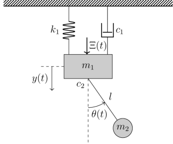
Figure 1: Block and pendulum

In this paper we consider the two-degree-of-freedom system shown in Figure 1. The primary system consists of a block of mass $m_{1}$ attached by a linear spring of stiffness $k_{1}$ and a viscous dashpot with a damping coefficient $c_{1}$. The block is excited directly by (downward) forcing $\Xi(t)$. The secondary system comprises a simple pendulum of length $\ell$ attached to the block. The mass of the pendulum bob is $m_{2}$ and the pendulum motion is damped by a viscous damper of coefficient $c_{2}$. This system appears in Hatwal, Mallik and Ghosh [12]. See also [4, 6] and a similar model with a non-linear spring and a compound pendulum in [32]. A closely related system with a vertically mounted cantilever beam with a tip mass appears in Haxton and Barr [13].

It is a characteristic property of an autoparametric system that there is a solution involving forced motion of the primary system while the secondary system remains at rest. Here it corresponds to the “single mode” solution in which the pendulum remains directly below the vibrating block at all times. As parameters in the system are varied, it may happen that the single mode solution becomes unstable and the pendulum begins to move. In this case the motion of the primary system causes excitation of the secondary system, and there is energy transfer from the vibrating block to the pendulum. In effect, the pendulum acts as a vibration absorber. Our primary concern is the almost-sure stability analysis of the single mode solution when the forcing function $\Xi(t)$ is a multiple of white noise.

In addition to the block and pendulum and block and beam examples mentioned above, autoparametric systems are used to model the dynamics of structural and mechanical systems such as the vibration of an initially deflected shallow arch [29], in-plane and out-of-plane motions of suspended cables [8], and the pitching and rolling motions of a ship [24, 26]. A larger collection of examples is given in the monograph [30].

Periodically excited autoparametric systems have been studied extensively; see for example [13, 25, 12, 9, 4, 6]. These are deterministic systems, and the most interesting situations occur when the natural frequencies of the primary (excited mode) and the secondary (unexcited) systems are in 2:1 resonance. Issues of bifurcation theory arise, and numerical computations frequently show chaotic behavior.

Autoparametric systems with stochastic forcing have also been studied. Gaussian and non-Gaussian closure techniques were used in [15, 27, 14, 10, 20] to approximate the moments of solutions of the associated Fokker-Planck equation. Sufficient conditions for almost-sure stability of the single mode solution were obtained in [1]. Stochastic averaging techniques were used in [23].

The equations of motion for the block and pendulum system shown in Figure 1 are

$$\begin{split}(m_{1}+m_{2})\ddot{y}(t)+c_{1}\dot{y}(t)+k_{1}y(t)-m_{1}\ell(\ddot{\theta}(t)\sin\theta(t)+{\dot{\theta}}^{2}(t)\cos\theta(t))&=\Xi(t)\\ m_{2}\ell^{2}\ddot{\theta}(t)+c_{2}\dot{\theta}(t)+m_{2}\ell(g-\ddot{y}(t))\sin\theta(t)&=0,\end{split}$$ (1.1)

where $y$ represents the downwards displacement of the block relative to its rest (unforced) position, and $\theta$ is the angle of the pendulum, see [12]. We specialize to the case of white noise forcing, that is $\Xi(t)=\hat{\nu}\dot{W}(t)$ where $W$ is a standard Wiener process and $\hat{\nu}$ represents the noise intensity.

Letting $\eta=y/\ell$ represent the dimensionless position of the block, the equations of motion (1.1) can be rewritten as

$$\begin{split}\ddot{\eta}(t)+2\zeta_{1}\dot{\eta}(t)+\chi^{2}\eta(t)-R\big{(}\ddot{\theta}(t)\sin{\theta}(t)+{\dot{\theta}}^{2}(t)\cos{\theta}(t)\big{)}&=\nu\dot{W}(t)\\ \ddot{\theta}(t)+2\zeta_{2}\dot{\theta}(t)+\big{(}\kappa^{2}-\ddot{\eta}(t)\big{)}\sin{\theta}(t)&=0,\end{split}$$ (1.2)

where the constants $\zeta_{1}$ and $\zeta_{2}$ are scaled damping coefficients, $\chi^{2}=k_{1}/(m_{1}+m_{2})$, and $\kappa=\sqrt{g/\ell}$ is the frequency of the undamped pendulum. The parameter $R=m_{2}/(m_{1}+m_{2})$, $0<R<1$, represents the mass ratio, and $\nu=\hat{\nu}/[\ell(m_{1}+m_{2})]$ is the scaled noise intensity.

The rigorous interpretation of (1.2) as a 4-dimensional stochastic differential equation (SDE) is carried out in Section 2. See Theorem 2.1 which guarantees existence and uniqueness and exponential moments for solutions with arbitrary initial conditions. The single mode solution of the system (1.2) is of the form

$$\big{(}\eta(t),\dot{\eta}(t)\big{)}=\big{(}\bar{\eta}(t),\dot{\bar{\eta}}(t)\big{)}\quad\text{and}\quad\big{(}\theta(t),\dot{\theta}(t)\big{)}=\big{(}0,0\big{)},$$ (1.3)

where the motion $\{(\bar{\eta}(t),\dot{\bar{\eta}}(t)):t\geq 0\}$ of the block is described by

$$\ddot{\bar{\eta}}(t)+2\zeta_{1}\dot{\bar{\eta}}(t)+\chi^{2}\bar{\eta}(t)=\nu\dot{W}(t).$$ (1.4)

The single mode (1.4) has a stationary solution $\{(\bar{\eta}(t),\dot{\bar{\eta}}(t)):t\geq 0\}$ with Gaussian stationary probability measure with mean $(0,0)$ and covariance matrix $R=\dfrac{\nu^{2}}{4\zeta_{1}}\begin{pmatrix}1/\chi^{2}&0\\ 0&1\end{pmatrix}$.

The stability or instability of the single mode solution is governed by the large time behavior of the process obtained by linearizing the 4-dimensional SDE along the single mode solution $(\bar{\eta}(t),\dot{\bar{\eta}}(t),0,0)$. In particular it is determined by the sign of the Lyapunov exponent

$$\lambda:=\lim\limits_{t\to\infty}\frac{1}{t}\log\|\left(\varphi(t),\dot{\varphi}(t)\right)\|$$ (1.5)

associated with the linear SDE

$$\ddot{\varphi}(t)+2\zeta_{2}\dot{\varphi}(t)+\big{(}\kappa^{2}+2\zeta_{1}\dot{\bar{\eta}}(t)+\chi^{2}\bar{\eta}(t)\big{)}\varphi(t)=\nu\varphi(t)\dot{W}(t)$$ (1.6)

where $(\bar{\eta}(t),\dot{\bar{\eta}}(t)$ is given by (1.4), see Section 2.1.

The novelty of the linear SDE (1.6) is that it is parametrically excited by the colored noise processes $\bar{\eta}(t)$ and $\dot{\bar{\eta}}(t)$ as well as the white noise (generalized) process $\dot{W}(t)$ which is driving them in (1.4). The techniques and results developed in this paper apply to a larger class of excitations of (1.6) consisting of combinations of Gaussian colored noise and white noise processes. This larger class is described in Section 3.

It is shown in Section 4 that the right side of (1.5) exists as an almost-sure limit, and is given by Khas’minskii’s integral formula (4.8) for all initial values $(\bar{\eta},\dot{\bar{\eta}},\varphi,\dot{\varphi})$ with $(\varphi,\dot{\varphi})\neq(0,0)$. Although the integrand $Q(v,\psi)$ in (4.8) is given explicitly, the measure $m$ is characterized only as the unique invariant probability measure for an associated diffusion process, and it is hard to evaluate the integral and obtain an exact formula for the Lyapunov exponent. However, assuming the pendulum is underdamped, so that the damped frequency $\kappa_{d}=\sqrt{\kappa^{2}-\zeta_{2}^{2}}$ is real and positive, a simple bound on $Q$ gives the following upper bound on the Lyapunov exponent,

$$\lambda\leq-\zeta_{2}+\frac{\nu}{2\kappa_{d}}\sqrt{\frac{\chi^{2}+4\zeta_{1}^{2}}{4\zeta_{1}}}+\frac{\nu^{2}}{2\kappa_{d}^{2}}.$$ (1.7)

see Proposition 4.2. This gives almost-sure stability for sufficiently small noise intensity $\nu$.

The main results in the paper are given in Section 5. Theorem 5.1 and Propositions 5.1 and 5.2 give rigorous asymptotic estimates for the Lyapunov exponent $\lambda(\varepsilon)$ for the system obtained when the noise intensity is rescaled $\nu\rightsquigarrow\varepsilon\nu$. For the block and pendulum system we show

$$\lambda(\varepsilon)=-\zeta_{2}+\varepsilon^{2}\frac{2\kappa_{d}^{2}\nu^{2}}{(\chi^{2}-4\kappa_{d}^{2})^{2}+16\zeta_{1}^{2}\kappa_{d}^{2}}+O(\varepsilon^{4})$$ (1.8)

as $\varepsilon\to 0$. Section 6 contains results in the case when the noise intensity and the pendulum damping are both rescaled: $\nu\rightsquigarrow\varepsilon\nu$ and $\zeta_{2}\rightsquigarrow\varepsilon^{2}\zeta_{2}$. There is a brief discussion of the similarities and differences in the 2:1 resonance effects for white noise and periodic forcing. The final three sections contain the proofs.

2 Well-posedness for the nonlinear system

Since $0<R<1$, the equations (1.2) can be rearranged to give

$$\begin{split}\ddot{\eta}(t)&+\frac{2\zeta_{1}\dot{\eta}(t)+\chi^{2}\eta(t)-R\dot{\theta}^{2}(t)\cos\theta(t)+2R\zeta_{2}\dot{\theta}(t)\sin\theta(t)+\kappa^{2}R\sin^{2}\theta(t)}{(1-R\sin^{2}\theta(t))}\\ &\hskip 172.22168pt=\frac{\nu}{(1-R\sin^{2}\theta(t))}\dot{W}(t)\\ \ddot{\theta}(t)&+\frac{2\zeta_{2}\dot{\theta}(t)+\kappa^{2}\sin\theta(t)+2\zeta_{1}\dot{\eta}(t)\sin\theta(t)+\chi^{2}\eta\sin\theta(t)-R\dot{\theta}^{2}(t)\sin\theta(t)\cos\theta(t)}{(1-R\sin^{2}\theta(t))}\\ &\hskip 172.22168pt=\frac{\nu\sin\theta(t)}{(1-R\sin^{2}\theta(t))}\dot{W}(t).\end{split}$$ (2.1)

This second order system for $(\eta,\theta)$ can now be turned into a first order system of stochastic differential equations for the process $(\eta,\dot{\eta},\theta,\dot{\theta})$ taking values in the space $N=\mathbb{R}^{2}\times\mathbb{R}/(2\pi\mathbb{Z})\times\mathbb{R}$. Write

$$(v_{1},v_{2},u_{1},u_{2})=(\eta,\dot{\eta},\theta,\dot{\theta}).$$

Then (2.1) gives

$$\begin{split}dv_{1}&=v_{2}\,dt\\ dv_{2}&=\frac{-2\zeta_{1}v_{2}-\chi^{2}v_{1}+Ru_{2}^{2}\cos u_{1}-2R\zeta_{2}u_{2}\sin u_{1}-R\kappa^{2}\sin^{2}u_{1}}{(1-R\sin^{2}u_{1})}dt\\ &\hskip 43.05542pt+\frac{\nu}{(1-R\sin^{2}u_{1})}dW(t)\\ du_{1}&=u_{2}\,dt\\ du_{2}&=\frac{-2\zeta_{2}u_{2}-\kappa^{2}\sin u_{1}-2\zeta_{1}v_{2}\sin u_{1}-\chi^{2}v_{1}\sin u_{1}+Ru_{2}^{2}\sin u_{1}\cos u_{1}}{(1-R\sin^{2}u_{1})}dt\\ &\hskip 43.05542pt+\frac{\nu\sin u_{1}}{(1-R\sin^{2}u_{1})}dW(t).\end{split}$$ (2.2)

We see that $du_{1}(t)dW(t)=0$ and so the Itô and Stratonovich interpretations of (2.2) are identical.

Let ${\cal L}$ denote the generator of the diffusion $\{(v_{1}(t),v_{2}(t),u_{1}(t),u_{2}(t)):t\geq 0\}$ given by (2.2). For ease of notation write $U(t)=(v_{1}(t),v_{2}(t),u_{1}(t),u_{2}(t))\in N$. Noting that $|u_{1}(t)|\leq 1$ we abuse notation by writing $\|U(t)\|=\sqrt{v_{1}^{2}(t)+v_{2}^{2}(t)+u_{2}^{2}(t)}$.

Theorem 2.1.

(i) For every initial condition $U(0)\in N$ the system (2.2) has a unique solution $\{U(t):t\geq 0\}$ valid for all $t\geq 0$.

(ii) There exists $b>0$ such that for every initial $U(0)$ the process $\{U(t):t\geq 0\}$ satisfies the condition $\|U(t)\|\leq b$ for infinitely many $t$ as $t\to\infty$.

(iii) There exist $\beta>0$ and $K$ such that every invariant probability $\pi$ for (2.2) satisfies

$$\int_{N}\exp\bigl{(}\beta\|U\|^{2}\bigr{)}d\pi(U)\leq K.$$

(iv) There exist $0<\beta\leq\beta_{1}$ and $K_{1}$ and for every $\gamma>0$ there exists $K_{2}$ such that

$$\mathbb{E}\exp\bigl{(}\beta\|U(t)\|^{2}\bigr{)}\leq K_{1}e^{-\gamma t}\exp\left(\beta_{1}\|U(0)\|^{2}\right)+K_{2}$$

for all initial conditions $U(0)\in N$ and all $t\geq 0$.

The proof of Theorem 2.1 is given in Section 7.

Remark 2.1.

The corresponding calculation for white noise forcing of the beam model discussed in [15, 27, 20] fails because it involves division by a term of the form $1-R\theta^{2}$ rather than $1-R\sin^{2}\theta$. There is no guarantee that the full non-linear system, for example [15, eqns (4,5)], has a solution valid for all time $t\geq 0$.

Remark 2.2.

Suppose that the simple pendulum is replaced by a compound pendulum with mass $m_{2}$, moment of inertia $I$ about the pivot point, and distance $d$ of the center of mass from the pivot point. The equations of motion are now

$$\begin{split}(m_{1}+m_{2})\ddot{y}(t)+c_{1}\dot{y}(t)+k_{1}y(t)-m_{2}d\bigl{(}\ddot{\theta}(t)\sin\theta(t)+{\dot{\theta}}^{2}(t)\cos\theta(t)\bigr{)}&=\Xi(t)\\ I\ddot{\theta}(t)+c_{2}\dot{\theta}(t)+m_{2}d(g-\ddot{y}(t))\sin\theta(t)&=0.\end{split}$$ (2.3)

Letting $\eta=y/L$ where $L=I/(m_{2}d)$ is the effective length of the compound pendulum the equations of motion (2.3) can be written in the form (1.2) where now $\kappa=\sqrt{g/L}$ is the frequency of the compound pendulum, and $R:=(d/L)\cdot m_{2}/(m_{1}+m_{2})<1$ because $L\geq d$.

There exists at least one stationary solution, the single mode solution described in (1.3,1.4) above. In addition there is an “unstable single mode” solution in which the pendulum is at rest directly above the block. It is described by (1.4) together with $(\theta(t),\dot{\theta}(t))=(\pi,0)$. There may or may not be other stationary solutions. We conjecture the existence of other “nonlinear” solutions depends on the stability of the single mode solution.

2.1 Stability of the single mode solution

In order to determine the stability of the single mode solution we study the long time behavior of the linearization of the system along the single mode solution (1.3,1.4). Writing $\eta(t)=\bar{\eta}(t)+\delta x(t)$ and $\theta(t)=0+\delta\varphi(t)$ in (1.2) and letting $\delta\to 0$ gives the set of variational equations:

$$\begin{split}\ddot{x}(t)+2\zeta_{1}\dot{x}(t)+\chi^{2}x(t)&=0\\ \ddot{\varphi}(t)+2\zeta_{2}\dot{\varphi}(t)+\big{(}\kappa^{2}-\ddot{\bar{\eta}}(t)\big{)}\varphi(t)&=0,\end{split}$$ (2.4)

where $\bar{\eta}_{t}$ is given by (1.4). More rigorously, linearizing the system (2.2) along the solution $(\bar{\eta},\dot{\bar{\eta}},0,0)$ gives a first order system for $(x,\dot{x},\varphi,\dot{\varphi})$ which is equivalent to

$$\begin{split}\ddot{x}(t)+2\zeta_{1}\dot{x}(t)+\chi^{2}x(t)&=0\\ \ddot{\varphi}(t)+2\zeta_{2}\dot{\varphi}(t)+\big{(}\kappa^{2}+2\zeta_{1}\dot{\bar{\eta}}(t)+\chi^{2}\bar{\eta}(t)\big{)}\varphi(t)&=\nu\varphi(t)\dot{W}(t).\end{split}$$ (2.5)

We see that the second line in (2.4) together with the information about $\bar{\eta}(t)$ in (1.4) is rigorously interpreted as the second line in (2.5).

The stability of the single mode solution is determined by the long time behavior of the linearized process $\{(x(t),\dot{x}(t),\varphi(t),\dot{\varphi}(t)):t\geq 0\}$. The top equation in (2.5) is damped and unforced, so $(x(t),\dot{x}(t))\to(0,0)$ as $t\to\infty$. Therefore it is enough to consider the parametric exitation of $\{(\varphi(t),\dot{\varphi}(t)):t\geq 0\}$ caused by the single mode vibration $\bar{\eta}$. For simplicity of notation we replace $\bar{\eta}$ with $\eta$ and consider the long term growth or decay rate for the process $\{(\varphi(t),\dot{\varphi}(t)):t\geq 0\}$ given by

$$\ddot{\eta}(t)+2\zeta_{1}\dot{\eta}(t)+\chi^{2}\eta(t) =\nu\dot{W}(t)$$ (2.6)

$$\ddot{\varphi}(t)+2\zeta_{2}\dot{\varphi}(t)+\big{(}\kappa^{2}+2\zeta_{1}\dot{\eta}(t)+\chi^{2}\eta(t)\big{)}\varphi(t) =\nu\varphi(t)\dot{W}(t),$$ (2.7)

The stability of the single mode solution is determined by the almost-sure exponential growth rate of (2.7), expressed precisely as the Lyapunov exponent

$$\lambda:=\lim\limits_{t\to\infty}\frac{1}{t}\log\|\left(\varphi(t),\dot{\varphi}(t)\right)\|.$$ (2.8)

We will see in Corollary 4.1 that the almost-sure limit in (2.8) exists and takes the same value for all initial conditions $(\eta(0),\dot{\eta}(0),\varphi(0),\dot{\varphi}(0))$ with $(\varphi(0),\dot{\varphi}(0))\neq(0,0)$.

Remark 2.3.

This paper concentrates on the well-posedness and evaluation of $\lambda$. The interpretation of $\lambda$, and especially of the sign of $\lambda$, should involve statements about the behavior of the original non-linear system (1.2). We conjecture that if $\lambda<0$ then all solutions with $(\varphi(0),\dot{\varphi}(0))\neq(\pi,0)$ converge to the single mode solution, and that if $\lambda>0$ then all solutions with $(\varphi(0),\dot{\varphi}(0))\not\in\{(0,0),(\pi,0)\}$ converge to a stationary solution with values in $\mathbb{R}^{2}\times\bigl{(}(\mathbb{R}/(2\pi\mathbb{Z})\times\mathbb{R})\setminus\{(0,0),(\pi,0)\}\bigr{)}$. In particular, if $\lambda<0$ then the single mode and the unstable single mode solutions are the only stationary solutions of (1.2), while if $\lambda>0$ then there is also a stationary solution satisfying $(\varphi(t),\dot{\varphi}(t))\not\in\{(0,0),(\pi,0)\}$ for all $t\geq 0$.

3 A more general linear system

Much of our analysis and computation of the Lyapunov exponent (2.8) is valid in a more general setting. Notice that (2.7) can be rewritten as

$$\ddot{\varphi}(t)+2\zeta_{2}\dot{\varphi}(t)+\bigl{(}\kappa^{2}-\ddot{\eta}(t)\bigr{)}\varphi(t)=0.$$ (3.1)

with $\eta(t)$ given by (2.6). We will replace the generalized process $\ddot{\eta}(t)$ by a more general $\xi(t)$.

Let $\{v(t):t\geq 0\}$ be the $\mathbb{R}^{d}$ valued Ornstein-Uhlenbeck process given by

$$dv(t)=Av(t)dt+BdW(t)$$ (3.2)

where $A$ is a $d\times d$ matrix, and $B$ is a $d\times m$ matrix and $W(t)$ is a standard $m$-dimensional Brownian motion. See for example Gardiner [11, Sect 4.4] or Liberzon and Brockett [21]. We shall assume throughout that the eigenvalues of $A$ have strictly negative real parts, and that $(A,B)$ is a controllable pair, that is

$$\mbox{rank}\{B,AB,\ldots,A^{d-1}B\}=d.$$ (3.3)

Since the eigenvalues of $A$ have strictly negative real parts, the equation (3.2) has a stationary solution

$$v(t)=\int_{-\infty}^{t}e^{(t-s)A}BdW(s)$$

with a stationary probability measure $\mu$, say, which is mean-zero Gaussian with $d\times d$ covariance matrix $R$ given by

$$R_{jk}=\sum_{\ell=1}^{m}\int_{-\infty}^{0}\bigl{(}e^{-sA}Be_{\ell}\bigr{)}_{j}\bigl{(}e^{-sA}Be_{\ell}\bigr{)}_{k}ds=\int_{0}^{\infty}\bigl{(}e^{tA}BB^{\ast}e^{tA^{\ast}}\bigr{)}_{jk}dt.$$ (3.4)

The controllable pair assumption is then equivalent to the assumption that $R$ is invertible, and this in turn is equivalent to the assumption that $\mbox{supp}(\mu)=\mathbb{R}^{d}$.

Choose $a\in\mathbb{R}^{d}$ and $\gamma\in\mathbb{R}^{m}$ and define

$$\xi(t)=\sum_{j=1}^{d}a_{j}v_{j}(t)+\sum_{\ell=1}^{m}\gamma_{\ell}\dot{W}_{\ell}(t)=\langle a,v(t)\rangle+\langle\gamma,\dot{W}(t)\rangle.$$ (3.5)

At the cost of replacing $m$ with $m+1$ and adjoining a column of zeroes to the matrix $B$, we can include the situation where $\xi(t)$ includes some white noise which is independent of the white noise driving $v(t)$. With this choice of $\xi(t)$ the equation

$$\ddot{\varphi}(t)+2\zeta_{2}\dot{\varphi}(t)+\bigl{(}\kappa^{2}-\xi(t)\bigr{)}\varphi(t)=0$$ (3.6)

has a well-defined meaning as the second order SDE

$$\ddot{\varphi}(t)+2\zeta_{2}\dot{\varphi}(t)+\bigl{(}\kappa^{2}-\langle a,v(t)\bigr{)}\varphi(t)=\sum_{\ell=1}^{m}\gamma_{\ell}\varphi(t)\dot{W}_{\ell}(t).$$ (3.7)

We will consider the Lyapunov exponent

$$\lambda:=\lim\limits_{t\to\infty}\frac{1}{t}\log\|\left(\varphi(t),\dot{\varphi}(t)\right)\|.$$ (3.8)

for the more general system given by (3.2,3.7).

Since $v(t)=\begin{pmatrix}\eta(t)\\ \dot{\eta}(t)\end{pmatrix}$ satisfies

$$dv(t)=\begin{pmatrix}0&1\\ -\chi^{2}&-2\zeta_{1}\end{pmatrix}v(t)dt+\begin{pmatrix}0\\ \nu\end{pmatrix}dW(t).$$ (3.9)

and

$$\ddot{\eta}(t)=-\chi^{2}\eta(t)-2\zeta_{1}\dot{\eta}(t)+\nu\dot{W}(t)$$

we see that the system (2.6,2.7) is a special case of (3.2,3.7).

4 Khas’minskii’s integral formula

Define $u(t)=\begin{pmatrix}\varphi(t)\\ \dot{\varphi}(t)\end{pmatrix}$, then (3.7) can be written as the 2-dimensional linear SDE

$$du(t)=\begin{pmatrix}0&1\\[4.30554pt] -\kappa^{2}+\langle a,v(t)\rangle&-2\zeta_{2}\end{pmatrix}u(t)dt+\sum_{\ell=1}^{m}\begin{pmatrix}0&0\\[4.30554pt] \gamma_{\ell}&0\end{pmatrix}u(t)dW_{\ell}(t).$$ (4.1)

We note that the Stratonovich and Itô interpretations of (4.1) are the same. Following Khas’minskii [18], write $u(t)=\|u(t)\|\begin{pmatrix}\cos\psi(t)\\ \sin\psi(t)\end{pmatrix}$. Applying Itô’s formula to (4.1) gives

$$d(\log\|u(t)\|)=Q(v(t),\psi(t))dt+\sum_{\ell=1}^{m}\gamma_{\ell}\sin\psi(t)\cos\psi(t)dW_{\ell}(t)$$

and

$$d\psi(t)=h(v(t),\psi(t))dt+\sum_{\ell=1}^{m}\gamma_{\ell}\cos^{2}\psi(t)dW_{\ell}(t)$$ (4.2)

where

$$Q(v,\psi)=\bigl{(}1-\kappa^{2}+\langle a,v\rangle\bigr{)}\sin\psi\cos\psi-2\zeta_{2}\sin^{2}\psi+\frac{\|\gamma\|^{2}}{2}\cos^{2}\psi\cos 2\psi$$ (4.3)

and

$$h(v,\psi)=-1+\bigl{(}1-\kappa^{2}+\langle a,v\rangle\bigr{)}\cos^{2}\psi-2\zeta_{2}\sin\psi\cos\psi-\|\gamma\|^{2}\sin\psi\cos^{3}\psi.$$

The process $\{(v(t),\psi(t)):t\geq 0\}$ given by (3.2,4.2) is a diffusion on $M:=\mathbb{R}^{d}\times\mathbb{R}/(2\pi\mathbb{Z})$ with generator ${\cal A}$, say. For $(\varphi(0),\dot{\varphi}(0))\neq(0,0)$ we have

$$\lim_{t\to\infty}\frac{1}{t}\log\sqrt{\varphi^{2}(t)+\dot{\varphi}^{2}(t)} =\lim_{t\to\infty}\frac{1}{t}\log\|u(t)\|$$

$$=\lim_{t\to\infty}\frac{1}{t}\left[\int_{0}^{t}Q(v(s),\psi(s))ds+\sum_{\ell=1}^{m}\int_{0}^{t}\frac{\gamma_{\ell}}{2}\sin 2\psi(s)\,dW_{\ell}(s)\right]$$ (4.4)

in the sense that the almost-sure existence and value of the limit on the left under initial conditions $(v,\varphi,\dot{\varphi})$ with $(\varphi,\dot{\varphi})\neq(0,0)$ is equivalent to the almost-sure existence and value of the limit on the right under initial conditions $(v,\psi)$.

Since

$$N(t)=\sum_{\ell=1}^{m}\int_{0}^{t}\frac{\gamma_{\ell}}{2}\sin 2\psi(s)\,dW_{\ell}(s)$$

is a continuous martingale with quadratic variation $\langle N\rangle_{t}\leq\|\gamma\|^{2}t/4$, it follows that

$$\mathbb{P}^{(v,\psi)}\left(\frac{1}{t}N(t)\to 0\mbox{ as }t\to\infty\right)=1$$ (4.5)

for all $(v,\psi)\in M$.

Proposition 4.1.

Assume that the eigenvalues of $A$ have strictly negative real parts, and that $(A,B)$ is a controllable pair. Assume also that the coefficients $a\in\mathbb{R}^{d}$ and $\gamma\in\mathbb{R}^{m}$ in (3.5) are not both zero. Then the diffusion $\{(v(t),\psi(t)):t\geq 0\}$ on $M$ has a unique stationary probability measure $m$, say, with smooth density $\rho(v,\psi)$. Moreover if $F:M\to\mathbb{R}$ is $m$ integrable then

$$\mathbb{P}^{(v,\psi)}\left(\frac{1}{t}\int_{0}^{t}F(v(s),\psi(s))ds\to\int_{M}F\,dm\mbox{ as }t\to\infty\right)=1$$ (4.6)

for every $(v,\psi)\in M.$

The proof of Proposition 4.1 is given in Section 8. The $v$ marginal of $m$ is the stationary probability measure $\mu$ on $\mathbb{R}^{d}$ which is mean-zero Gaussian with mean zero and covariance matrix $R$ given by (3.4). There exist constants $k_{0}$ and $k_{1}$ such that $|Q(v,\psi)|\leq k_{0}+k_{1}\|v\|$ and so

$$\int_{M}|Q(v,\psi)|dm(v,\psi)\leq\int_{\mathbb{R}^{d}}\bigl{(}k_{0}+k_{1}\|v\|\bigr{)}d\mu(v)<\infty.$$

By (4.4) and (4.5) and using Proposition 4.1 we obtain

Corollary 4.1.

(i) Under the assumptions of Proposition 4.1 we have

$$\mathbb{P}^{(v,\varphi,\dot{\varphi})}\left(\frac{1}{t}\log\|(\varphi(t),\dot{\varphi}(t))\|\to\int_{M}Q\,dm\mbox{ as }t\to\infty\right)=1$$ (4.7)

for every $(v,\varphi,\dot{\varphi})$ with $(\varphi,\dot{\varphi})\neq(0,0)$.

(ii) The Lyapunov exponent $\lambda$ defined in (3.8) exists as an almost-sure limit for all initial conditions $(v,\varphi,\dot{\varphi})$ with $(\varphi,\dot{\varphi})\neq(0,0)$ and

$$\lambda=\int_{M}Q(v,\psi)\,dm(v,\psi).$$ (4.8)

4.1 Evaluation

Direct evaluation of (4.8) is hard, because we need to first solve ${\cal A}^{\ast}m=0$. There is a simple case when $a=0$, because then $v(t)$ disappears from (4.1) and problem reduces to a constant coefficient linear SDE in $\mathbb{R}^{2}$. In this case the exact formula of Imkeller and Lederer [17] will apply. But this excludes the original block-pendulum model. The block-pendulum case is interesting because of the different sorts of noise in (2.7): white noise $\dot{W}(t)$ as well as colored noise $\eta(t)$ and $\dot{\eta}(t)$.

Before proceeding to the small noise estimates, we give a simple upper bound for the Lyapunov exponent $\lambda$.

Proposition 4.2.

Assume $\zeta_{2}<\kappa$ and let $\kappa_{d}=\sqrt{\kappa^{2}-\zeta_{2}^{2}}$ denote the damped frequency of the pendulum. Then

$$\lambda\leq-\zeta_{2}+\frac{\sqrt{\langle a,Ra\rangle}}{2\kappa_{d}}+\frac{\|\gamma\|^{2}}{2\kappa_{d}^{2}},$$ (4.9)

where $R$ is the covariance matrix (3.4). For the original block and pendulum setting

$$\lambda\leq-\zeta_{2}+\frac{\nu}{2\kappa_{d}}\sqrt{\frac{\chi^{2}+4\zeta_{1}^{2}}{4\zeta_{1}}}+\frac{\nu^{2}}{2\kappa_{d}^{2}}.$$ (4.10)

The proof of Proposition 4.2 uses a slightly different version of the function $Q(v,\psi)$ and is given in Section 9.1. The result is motivated by an estimate in Ariaratnam [1].

5 Small forcing

In this section we consider the effect of small forcing of the block. Precisely, we replace $\nu\rightsquigarrow\varepsilon\nu$ for small $\varepsilon$. The linearized system (2.6,2.7) becomes

$$\ddot{\eta}(t)+2\zeta_{1}\dot{\eta}(t)+\chi^{2}\eta(t) =\varepsilon\nu\dot{W}(t),$$

$$\ddot{\varphi}(t)+2\zeta_{2}\dot{\varphi}(t)+\big{(}\kappa^{2}+2\zeta_{1}\dot{\eta}(t)+\chi^{2}\eta(t)\big{)}\varphi(t) =\varepsilon\nu\varphi(t)\dot{W}(t).$$

Equivalently, writing $\eta(t)=\varepsilon\tilde{\eta}(t)$ and then dropping the tilde

$$\ddot{\eta}(t)+2\zeta_{1}\dot{\eta}(t)+\chi^{2}\eta(t) =\nu\dot{W}(t),$$ (5.1)

$$\ddot{\varphi}(t)+2\zeta_{2}\dot{\varphi}(t)+\big{(}\kappa^{2}+2\varepsilon\zeta_{1}\dot{\eta}(t)+\varepsilon\chi^{2}\eta(t)\big{)}\varphi(t) =\varepsilon\nu\varphi(t)\dot{W}(t).$$ (5.2)

For the more general problem in Section 3 we replace $\xi(t)\rightsquigarrow\varepsilon\xi(t)$ in (3.6), that is $a\rightsquigarrow\varepsilon a$ and $\gamma\rightsquigarrow\varepsilon\gamma$, giving the equation

$$\ddot{\varphi}(t)+2\zeta_{2}\dot{\varphi}(t)+\big{(}\kappa^{2}-\varepsilon\langle a,v(t)\rangle\big{)}\varphi(t)=\sum_{\ell=1}^{m}\varepsilon\gamma_{\ell}\varphi(t)\dot{W}_{\ell}(t)$$ (5.3)

where $\{v(t):t\geq 0\}$ is still given by (3.2). We now define the Lyapunov exponent

$$\lambda(\varepsilon):=\lim\limits_{t\to\infty}\frac{1}{t}\log\|\left(\varphi(t),\dot{\varphi}(t)\right)\|.$$ (5.4)

where $\{\varphi(t):t\geq 0\}$ is given by (5.3).

Define the matrix valued cosine transform of $A$ by

$$\widehat{S}_{A}(\omega)=\frac{1}{\pi}\int_{0}^{\infty}e^{tA}\cos\omega t\,dt,$$ (5.5)

and recall that $R$ denotes the covariance matrix of the stationary probability measure $\mu$ for $\{v(t):t\geq 0\}$.

Theorem 5.1.

(i) Assume that the eigenvalues of $A$ have strictly negative real parts, and that $(A,B)$ is a controllable pair. Assume $\zeta_{2}<\kappa$ and let $\kappa_{d}=\sqrt{\kappa^{2}-\zeta_{2}^{2}}$ denote the damped frequency of the pendulum. For $\{\varphi(t):t\geq 0\}$ given by (5.3) we have

$$\lambda(\varepsilon)=-\zeta_{2}+\varepsilon^{2}\lambda_{2}(2\kappa_{d})+O(\varepsilon^{4})\quad\mbox{ as }\varepsilon\to 0.$$ (5.6)

where

$$\lambda_{2}(\omega)=\frac{\pi}{\omega^{2}}\Bigl{(}\langle a,\widehat{S}_{A}(\omega)Ra\rangle+\langle a,\widehat{S}_{A}(\omega)B\gamma\rangle+\frac{\|\gamma\|^{2}}{2\pi}\Bigr{)}.$$ (5.7)

(ii) Moreover, given matrices $A$ and $B$ and vectors $a$ and $\gamma$ the asymptotic (5.6) is uniform for $\kappa_{d}$ bounded away from 0 and $\infty$. That is, given $A$, $B$, $a$, $\gamma$ and $0<c_{1}<c_{2}<\infty$ there exists $K$ such that

$$\Bigl{|}\lambda(\varepsilon)+\zeta_{2}-\varepsilon^{2}\lambda_{2}(2\kappa_{d})\Bigr{|}\leq K\varepsilon^{4}$$ (5.8)

whenever $0<\varepsilon\leq 1$ and $c_{1}\leq\kappa_{d}\leq c_{2}$.

The proof for Theorem 5.1 is given in Section 9.

Observe that the destabilizing effect of the noise is strongest when the damped frequency $\kappa_{d}$ maximises the function $\lambda_{2}(2\omega)$. We will expand on this observation in Section 6.

5.1 Evaluation of $\lambda_{2}(\omega)$

In the special case when $a=0$ we have $\lambda_{2}(\omega)=\|\gamma\|^{2}/(2\omega^{2})$ and we recover the result of Auslender and Milstein [3] that

$$\lambda(\varepsilon)=-\zeta_{2}+\frac{\varepsilon^{2}\|\gamma\|^{2}}{8\kappa_{d}^{2}}+O(\varepsilon^{4})\quad\mbox{ as }\varepsilon\to 0.$$

But when $a\neq 0$ we have to do some work to simplify the formula (5.7) for $\lambda_{2}(\omega)$. The covariance matrix $R$ is determined by (3.4). The cosine transform $\widehat{S}_{A}(\omega)$ defined in (5.5) satisfies

$$\widehat{S}_{A}(\omega)=\frac{1}{\pi}\Re\Bigl{(}\int_{0}^{\infty}e^{tA}e^{-i\omega t}\,dt\Bigr{)}=-\frac{1}{\pi}\Re\Bigl{(}(A-i\omega I_{d})^{-1}\Bigr{)}.$$ (5.9)

Hence, given the matrices $A$ and $B$ and the vectors $a$ and $\gamma$, all the terms in (5.7) can be calculated.

We will give formulas for $\lambda_{2}(\omega)$ in terms of power spectral density. Recall that for any $L^{2}$ stationary mean zero scalar process $X(t)$ the power spectral density function $S_{X}$ is given by

$$S_{X}(\omega)=\frac{1}{2\pi}\int_{-\infty}^{\infty}\mathbb{E}[X(t)X(0)]e^{-i\omega t}\,dt=\frac{1}{\pi}\int_{0}^{\infty}\mathbb{E}[X(t)X(0)]\cos\omega t\,dt.$$ (5.10)

We note that many authors omit the factor $1/2\pi$.

The block and pendulum setting has $\xi(t)=\ddot{\eta}(t)$ where $\dot{\eta}(t)$ is a well-defined $L^{2}$ stationary process. The first result extends this case to the general system of Section 3.

Fix $\alpha\in\mathbb{R}^{d}$ and define $\xi(t)=\dot{V}(t)$ where $V(t)=\langle\alpha,v(t)\rangle$. Since

$$\xi(t)=\langle\alpha,\dot{v}(t)\rangle=\langle\alpha,Av(t)\rangle+\langle\alpha,B\dot{W}(t)\rangle=\langle A^{\ast}\alpha,v(t)\rangle+\langle B^{\ast}\alpha,\dot{W}(t)\rangle,$$ (5.11)

we have (3.5) with $a=A^{\ast}\alpha$ and $\gamma=B^{\ast}\alpha$. Note that $V(t)$ is a well-defined $L^{2}$ stationary process, so that it has a well-defined autocovariance function $\mathbb{E}[V(t)V(0)]$ and hence a well-defined power spectral density $S_{V}(\omega)$ using the formula (5.10).

Proposition 5.1.

For $\xi$ given by 5.11 we have

$$\lambda_{2}(\omega)=\pi S_{V}(\omega).$$ (5.12)

Specializing to the original block and pendulum case, we have $\xi(t)=\ddot{\eta}(t)=\dot{v_{2}}(t)$ where $v(t)=\begin{pmatrix}\eta(t)\\ \dot{\eta}(t)\end{pmatrix}$ as in (3.9). Therefore we may apply Proposition 5.1 with $V(t)=v_{2}(t)=\dot{\eta}(t)$. For the system (3.9) the power spectral density $S_{\dot{\eta}}(w)$ is well known, see for example [11, Sect.4.4].

Corollary 5.1.

For $\xi=\ddot{\eta}$ given by 2.6 we have

$$\lambda_{2}(\omega)=\pi S_{\dot{\eta}}(\omega)=\frac{\omega^{2}\nu^{2}}{2[(\chi^{2}-\omega)^{2}+4\zeta_{1}^{2}\omega^{2}]}.$$ (5.13)

In the general case (3.5) when $\xi(t)=\langle a,v(t)\rangle+\langle\gamma,\dot{W}(t)\rangle$ with $\gamma\neq 0$ then $\xi$ is not a well-defined $L^{2}$ process. It does not have an autocovariance function, and the formula (5.10) for the power spectral density does not apply. However we can consider the power spectral density $S_{\xi_{\delta}}(\omega)$ for a mollified version $\xi_{\delta}$ of $\xi$.

Suppose $\psi:\mathbb{R}\to[0,\infty)$ is piecewise continuous with support in $[-1,1]$ and
$\int_{-\infty}^{\infty}\psi(t)dt=1$. Define $\psi_{\delta}(t)=(1/\delta)\psi(t/\delta)$. For any continuous function $f$ we have

$$f_{\delta}(t):=f\ast\psi_{\delta}(t)=\int_{-\infty}^{\infty}f(s)\psi_{\delta}(t-s)ds=\int_{-\infty}^{\infty}f(t-\delta u)\psi(u)du\to f(t)$$ (5.14)

as $\delta\to 0$, so that the functions $\psi_{\delta}(t-\cdot)$ converge to the Dirac delta distribution at $t$. Then the process $\xi_{\delta}$ defined informally as $\xi*\psi_{\delta}$ and precisely by

$$\xi_{\delta}(t)=\int_{-\infty}^{\infty}\langle a,v(s)\rangle\psi_{\delta}(t-s)ds+\left\langle\gamma,\int_{-\infty}^{\infty}\psi_{\delta}(t-s)dW(s)\right\rangle$$ (5.15)

is well-defined $L^{2}$ process, and it converges in a weak sense to the generalized process $\xi$.

Proposition 5.2.

For $\xi(t)=\langle a,v(t)\rangle+\langle\gamma,\dot{W}(t)\rangle$ and $\xi_{\delta}(t)$ given by (5.15) the limit

$$\lim_{\delta\to 0}S_{\xi_{\delta}}(\omega)=\langle a,\widehat{S}_{A}(\omega)Ra\rangle+\langle a,\widehat{S}_{A}(\omega)B\gamma\rangle+\frac{\|\gamma\|^{2}}{2\pi}$$ (5.16)

exists and does not depend on the choice of $\psi$. Defining $S_{\xi}(\omega):=\lim_{\delta\to 0}S_{\xi_{\delta}}(\omega)$ we have

$$\lambda_{2}(\omega)=\frac{\pi}{\omega^{2}}S_{\xi}(\omega).$$ (5.17)

The proofs of Propositions 5.1 and 5.2 are given in Section 9.

6 Small forcing and small pendulum damping

In this section we consider the combined effect of small forcing of the block together with small damping of the pendulum. Precisely, we replace

$$\nu\rightsquigarrow\varepsilon\nu\quad\mbox{ and }\quad\zeta_{2}\rightsquigarrow\varepsilon^{2}\zeta_{2}$$

for small $\varepsilon$. The equation for $\varphi$ is now

$$\ddot{\varphi}(t)+2\varepsilon^{2}\zeta_{2}\dot{\varphi}(t)+\big{(}\kappa^{2}+2\varepsilon\zeta_{1}\dot{\eta}(t)+\varepsilon\chi^{2}\eta(t)\big{)}\varphi(t)=\varepsilon\nu\varphi(t)\dot{W}(t)$$ (6.1)

for the original block and pendulum setting, and

$$\ddot{\varphi}(t)+2\varepsilon^{2}\zeta_{2}\dot{\varphi}(t)+\big{(}\kappa^{2}-\varepsilon\langle a,v(t)\rangle\big{)}\varphi(t)=\sum_{\ell=1}^{m}\varepsilon\gamma_{\ell}\varphi(t)\dot{W}_{\ell}(t)$$ (6.2)

in the general setting. In order to distinguish this scaling from the previous one in Section 5 we write

$$\widehat{\lambda}(\varepsilon):=\lim\limits_{t\to\infty}\frac{1}{t}\log\|\left(\varphi(t),\dot{\varphi}(t)\right)\|.$$ (6.3)

for the Lyapunov exponent where $\{\varphi(t):t\geq 0\}$ is given by (6.2).

Theorem 6.1.

Assume that the eigenvalues of $A$ have strictly negative real parts, and that $(A,B)$ is a controllable pair. For the process $\big{\{}\big{(}\varphi(t),\dot{\varphi}(t)\big{)}:t\geq 0\big{\}}$ given by (6.2) we have

$$\widehat{\lambda}(\varepsilon)=\varepsilon^{2}\bigl{(}-\zeta_{2}+\lambda_{2}(2\kappa)\bigr{)}+O(\varepsilon^{4})\quad\mbox{ as }\varepsilon\to 0.$$ (6.4)

where $\lambda_{2}(\omega)$ is given by (5.7).

Proof.

The damped frequency for (6.2) is $\kappa_{d}=\sqrt{\kappa^{2}-\varepsilon^{4}\zeta_{2}^{4}}=\kappa+O(\varepsilon^{4})$, and so $\lambda_{2}(2\kappa_{d})=\lambda_{2}(2\kappa)+O(\varepsilon^{4})$. The result now follows directly from Theorem 5.1(ii). ∎

Returning to the original block and pendulum case and using (5.13) we have

$$\widehat{\lambda}(\varepsilon)=\varepsilon^{2}\left(-\zeta_{2}+\frac{2\nu^{2}\kappa^{2}}{(\chi^{2}-4\kappa^{2})^{2}+16\zeta_{1}^{2}\kappa^{2}}\right)+O(\varepsilon^{4})\quad\mbox{ as }\varepsilon\to 0.$$ (6.5)

Recall that the long term exponential growth or decay rate for the process $\big{\{}\big{(}\varphi(t),\dot{\varphi}(t)\big{)}:t\geq 0\big{\}}$ is given by the Lyapunov exponent $\widehat{\lambda}(\varepsilon)$. Putting $\widehat{\lambda}(\varepsilon)=0$ in (6.5) provides the almost-sure stability boundary in terms of the excitation intensity $\nu$. Hence the second order approximation of the almost-sure stability boundary is given by

$$\nu_{c}^{2}=\frac{\zeta_{2}\big{[}(\chi^{2}-4\kappa^{2})^{2}+16\zeta_{1}^{2}\kappa^{2}\big{]}}{2\kappa^{2}}=\zeta_{2}\left(\frac{(\chi^{2}-4\kappa^{2})^{2}}{2\kappa^{2}}+8\zeta_{1}^{2}\right).$$ (6.6)

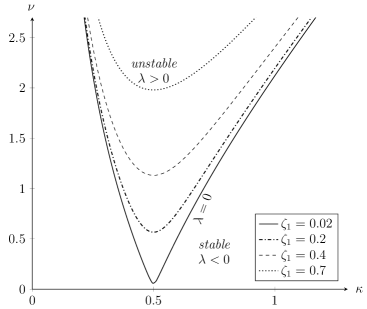
Figure 2: Almost-sure stability boundaries with $\chi=1$ and $\zeta_{2}=1$ and $\zeta_{1}=0.02$, 0.2, 0.4 and 0.7.

It is clear that the dissipation in both the primary ($\zeta_{1}$) and secondary ($\zeta_{2}$) systems has a stabilizing effect on the single mode solution. Although no particular attention was given to the $1:2$ resonance in the analysis of the linearized system, the stability boundary (6.6) shows the significance of internal resonance, $\chi\approx 2\kappa$, in determining the instability region in the $(\kappa,\nu)$ parameter space, which is of significance in applications. For fixed $\chi$, $\zeta_{1}$ and $\zeta_{2}$ the critical noise intensity $\nu_{c}$, as a function of $\kappa$, has a minumum value $\sqrt{8\zeta_{1}^{2}\zeta_{2}}$ attained when $\kappa=\chi/2$. Figure 2 shows $\nu_{c}$ as a function of $\kappa$ with $\chi=1$ and $\zeta_{2}=1$ and $\zeta_{1}=0.02$, 0.2, 0.4 and 0.7.

The behavior displayed in Figure 2 mimics that of the instability tongues and transition curves in the stability chart for Mathieu’s equation with linear viscous damping and cosine periodic forcing. More specifically the equation

$$\ddot{\varphi}(t)+2\varepsilon\zeta_{2}\dot{\varphi}(t)+(\kappa^{2}-\varepsilon\nu\cos\omega t)\varphi(t)=0$$ (6.7)

with small periodic forcing $\varepsilon\nu$ and small dissipation $\varepsilon\zeta_{2}$ has first order approximation (as $\varepsilon\to 0$) of the stability boundary given by

$$\varepsilon^{2}(\nu_{c}^{2}-16\zeta_{2}^{2})=\omega^{2}\left(\frac{4\kappa^{2}}{\omega^{2}}-1\right)^{2}.$$ (6.8)

See Verhulst [31, page 241] for the case $\omega=2$. Note that in the deterministic setting the damping is of the same order $\varepsilon$ as the forcing. Figure 3 shows $\nu_{c}$ as a function of $\kappa$ with $\omega=1$, $\zeta_{2}=0.1$ and $\varepsilon=0.2$, 0.1 and 0.05. Notice that in this model the “width” of the instability region decreases as $\varepsilon$ decreases.

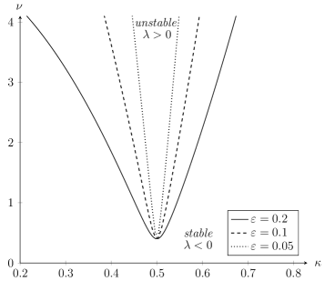
Figure 3: Almost-sure stability boundaries for the Mathieu equation (6.7) with $\omega=1$, $\zeta_{2}=0.1$ and $\varepsilon=0.2$, 0.1 and 0.05.

A more directly relevant comparison is seen when we replace white noise forcing in the autoparametric system with periodic (deterministic) forcing. Consider the system

$$\begin{split}\ddot{\eta}(t)+2\zeta_{1}\dot{\eta}(t)+\chi^{2}\eta(t)-R\big{(}\ddot{\theta}(t)\sin{\theta}(t)+{\dot{\theta}}^{2}(t)\cos{\theta}(t)\big{)}&=\varepsilon\nu\cos\omega t\\ \ddot{\theta}(t)+2\varepsilon\zeta_{2}\dot{\theta}(t)+\big{(}\kappa^{2}-\ddot{\eta}(t)\big{)}\sin{\theta}(t)&=0,\end{split}$$ (6.9)

with forcing of some fixed frequency $\omega$ and small intensity $\varepsilon\nu$, and small pendulum damping $\varepsilon\zeta_{2}$. Linearizing along the single mode solution $\theta(t)\equiv 0$ we get

$$\ddot{\eta}(t)+2\zeta_{1}\dot{\eta}(t)+\chi^{2}\eta(t) =\varepsilon\nu\cos\omega t$$ (6.10)

$$\ddot{\varphi}(t)+2\varepsilon\zeta_{2}\dot{\varphi}(t)+\bigl{(}\kappa^{2}-\ddot{\eta}(t)\bigr{)}\varphi(t) =0.$$ (6.11)

The stationary solution of (6.10) is

$$\eta(t)=\frac{\varepsilon\nu}{\sqrt{(\chi^{2}-\omega^{2})^{2}+4\zeta_{1}^{2}\omega^{2}}}\cos(\omega t+\alpha)$$

where $\alpha=\mbox{arg}(\chi^{2}-\omega^{2}+2i\zeta_{1}\omega)$, and so

$$\ddot{\eta}(t)=\frac{\varepsilon\omega^{2}\nu}{\sqrt{(\chi^{2}-\omega^{2})^{2}+4\zeta_{1}^{2}\omega^{2}}}\cos(\omega t+\alpha+\pi).$$

Therefore (6.11) has the form of Mathieu’s equation (6.7) with $\nu$ replaced by $\dfrac{\omega^{2}\nu}{\sqrt{(\chi^{2}-\omega^{2})^{2}+4\zeta_{1}^{2}\omega^{2}}}$. The phase change $\pi+\alpha$ has no effect on the stability, and the (first order) stability boundary is

$$\varepsilon^{2}\left(\frac{\omega^{4}\nu_{c}^{2}}{(\chi^{2}-\omega^{2})^{2}+4\zeta_{1}^{2}\omega^{2}}-16\zeta_{2}^{2}\right)=\omega^{2}\left(\frac{4\kappa^{2}}{\omega^{2}}-1\right)^{2}.$$ (6.12)

A multiplicative change in the vertical coordinate will convert the stability regions for the Mathieu equation (6.7) shown in Figure 3 into the corresponding regions for the periodically forced autoparametric system (6.10,6.11).

Remark 6.1.

For the periodically forced system (6.10,6.11) the functions $\eta(t)$ and $\ddot{\eta}(t)$ are related by a simple multiplicative factor. It makes little theoretical difference whether $\nu\cos\omega t$ is applied as forcing on the block, or is assumed to describe the motion of the pivot point. The situation with stochastic forcing is very different. With white noise forcing $\{\eta(t):t\geq 0\}$ is an $L^{2}$ process with continous sample paths, whereas $\{\ddot{\eta}(t):t\geq 0\}$ exists only as a generalized process and has to be interpreted in terms of stochastic integrals.

7 Proof of Theorem 2.1

7.1 Construction of a Lyapunov function

Up to normalization, the energy of the block and pendulum system is given by

$$E(v_{1},v_{1},u_{1},u_{2})=\frac{1}{2}v_{2}^{2}+\frac{1}{2}Ru_{2}^{2}-Rv_{2}u_{2}\sin u_{1}+\frac{1}{2}\chi^{2}v_{1}^{2}+R\kappa^{2}(1-\cos u_{1}).$$ (7.1)

Lemma 7.1.

$${\cal L}E(v_{1},v_{1},u_{1},u_{2})=-2\zeta_{1}v_{2}^{2}-2R\zeta_{2}u_{2}^{2}+\frac{\nu^{2}}{2(1-R\sin^{2}u_{1})}.$$

$${\cal L}\Bigl{(}v_{1}(v_{2}-Ru_{2}\sin u_{1})\Bigr{)}=v_{2}^{2}-Rv_{2}u_{2}\sin u_{1}-2\zeta_{1}v_{1}v_{2}-\chi^{2}v_{1}^{2}.$$

Proof.

This is direct calculation. ∎

For $\alpha$ to be chosen later, define

$$F(v_{1},v_{2},u_{1},u_{2})=E(v_{1},v_{1},u_{1},u_{2})+\alpha\Bigl{(}v_{1}(v_{2}-Ru_{2}\sin u_{1})\Bigr{)}.$$ (7.2)

Proposition 7.1.

(i) There exist $\alpha>0$ and positive constants $c_{1},\ldots,c_{5}$ such that

$$c_{1}\|(v_{1},v_{2},u_{2})\|^{2}\leq F(v_{1},v_{2},u_{1},u_{2})\leq c_{2}+c_{3}\|(v_{1},v_{2},u_{2})\|^{2}$$ (7.3)

and

$${\cal L}F(v_{1},v_{2},u_{1},u_{2})\leq c_{4}-c_{5}\|(v_{1},v_{2},u_{2})\|^{2}.$$ (7.4)

(ii) For $\alpha>0$ as in (i), there exists $\beta_{0}>0$ such that for all $\gamma>0$ there exists $c_{6}$ such that

$${\cal L}(e^{\beta_{0}F(v_{1},v_{2},u_{1},u_{2})})\leq-\gamma e^{\beta_{0}F(v_{1},v_{2},u_{1},u_{2})}+c_{6}.$$ (7.5)

Proof.

(i) Several applications of the Cauchy-Schwarz inequality give

$$\frac{1-\sqrt{R}}{2}(v_{2}^{2}+Ru_{2}^{2})+\frac{1}{2}\chi^{2}v_{1}^{2}-\alpha\Bigl{(}v_{1}^{2}+\frac{1}{2}v_{2}^{2}+\frac{1}{2}R^{2}u_{2}^{2}\Bigr{)}$$

$$\hskip 43.05542pt\leq F(v_{1},v_{2},u_{1},u_{2})$$

$$\hskip 43.05542pt\leq R\kappa^{2}+\frac{1+\sqrt{R}}{2}(v_{2}^{2}+Ru_{2}^{2})+\frac{1}{2}\chi^{2}v_{1}^{2}+\alpha\Bigl{(}v_{1}^{2}+\frac{1}{2}v_{2}^{2}+\frac{1}{2}R^{2}u_{2}^{2}\Bigr{)}.$$

Thus the upper and lower bounds on $F$ are satisfied whenever $0<\alpha<\min(1-\sqrt{R},\chi^{2}/2)$.

Similarly, using Lemma 7.1,

$${\cal L}F(v_{1},v_{2},u_{1},u_{2}) \leq\frac{\nu^{2}}{2(1-R)}-2\zeta_{1}v_{2}^{2}-2R\zeta_{2}u_{2}^{2}+\alpha\Bigl{(}v_{2}^{2}+R|v_{2}u_{2}|+2\zeta_{1}|v_{1}v_{2}|-\chi^{2}v_{1}^{2}\Bigr{)}$$

$$\leq\frac{\nu^{2}}{2(1-R)}-2\zeta_{1}v_{2}^{2}-2R\zeta_{2}u_{2}^{2}+\frac{\alpha}{2}\Bigl{(}(2+R+\frac{4\zeta_{1}^{2}}{\chi^{2}})v_{2}^{2}+Ru_{2}^{2}-\chi^{2}v_{1}^{2}\Bigr{)}.$$

The upper bound on ${\cal L}F$ now follows by choosing $\alpha$ sufficiently small.

(ii) Let $\Gamma$ denote the carré du champ operator associated with ${\cal L}$, see for example [5]. Since $\partial F/dv_{2}$ and $\partial F/du_{2}$ both grow at most linearly with $\|(v_{1},v_{2},u_{2})\|$ and the coefficients of $dW(t)$ in (2.2) are bounded, there exists $c_{7}$ such that $\Gamma(F,F)\leq c_{7}\|(v_{1},v_{2},u_{2})\|^{2}$. Then

$${\cal L}\left(e^{\beta_{0}F}\right) =\Bigl{(}\beta_{0}{\cal L}F+\beta_{0}^{2}\Gamma(F,F)\Bigr{)}e^{\beta_{0}F}$$

$$\leq\Bigl{(}\beta_{0}(c_{4}-c_{5}\|(v_{1},v_{2},u_{2})\|^{2})+\beta_{0}^{2}c_{7}\|(v_{1},v_{2},u_{2})\|^{2}\Bigr{)}e^{\beta_{0}F}$$

$$=\Bigl{(}\beta_{0}c_{4}-\beta_{0}(c_{5}-\beta_{0}c_{7})\|(v_{1},v_{2},u_{2})\|^{2}\Bigr{)}e^{\beta_{0}F}.$$

Choose $\beta_{0}>0$ so that $\beta_{0}c_{7}<c_{5}$. For each $\gamma>0$ there a radius $r$ such that ${\cal L}(e^{\beta_{0}F})\leq-\gamma e^{\beta_{0}F}$ if $\|(v_{1},v_{2},u_{2})\|\geq r$, and of course ${\cal L}(e^{\beta_{0}F})$ is bounded in the set $\|(v_{1},v_{2},u_{2})\|\leq r$. ∎

7.2 Consequences of the Lyapunov function

Recall the notation $(v_{1},v_{2},u_{1},u_{2})=U\in N$ and the abuse of notation $\|(v_{1},v_{2},u_{2})\|=\|U\|$. Fix $\alpha$ and $\beta$ so that the results of Proposition 7.1 are valid for the function $F$.

Proof of Theorem 2.1(i). The coefficients of (2.2) are locally Lipschitz, so there is a well-defined local solution. Proposition 7.1 implies $F(U)\to\infty$ as $\|U\|\to\infty$, and there exists $c$ such that ${\cal L}(1+F)(U)\leq c(1+F)(U)$ for all $U$. The result of Khas’minskii [19, Thm 3.5] implies that the well-defined local solution exists for all time and is a Feller process.

Proof of Theorem 2.1(ii). Notice that if $0<c<c_{5}$ and $d=c_{4}+c$ and $b^{2}=(c_{4})/(c_{5}-c)$ then

$${\cal L}F(U)\leq c_{4}-c_{5}\|U\|^{2}\leq-c(1+\|U\|^{2})+d1_{\|U\|\leq b}$$

This gives condition (CD2) of Meyn and Tweedie [22]. It now follows from [22, Thm 4.3(i)] that $\mathbb{P}(\|U_{t}\|\leq b\mbox{ for some }t\geq\delta)=1$ for all initial conditions $U(0)$ and all $\delta>0$.

Proof of Theorem 2.1(iii). The inequality (7.5) implies that $e^{\beta_{0}F}$ satisfies condition (CD2) of [22]. Taking $\beta=c_{1}\beta_{0}$ and using (7.3) for the first inequality, and then [22, Th 4.3(ii)] for the second inequality gives

$$\int_{N}\exp\bigl{(}\beta\|U\|^{2}\bigr{)}d\pi(U)\leq\int_{N}\exp\bigl{(}\beta_{0}F(U)\bigr{)}d\pi(U)\leq\frac{c_{6}}{\gamma}$$

for every invariant probability measure $\pi$ for (2.2).

Proof of Theorem 2.1(iv). The function $e^{\beta_{0}F}$ also satisfies condition (CD3) of [22], so by the calculation in the proof of [22, Thm 6.1] we have

$$\mathbb{E}[e^{\beta_{0}F(U_{t})}]\leq e^{-\gamma t}e^{\beta_{0}F(U)}+\frac{c_{6}}{\gamma}.$$

It remains only to use the upper and lower bounds on $F(U)$ given in (7.3). We have $\beta=c_{1}\beta_{0}$ and $\beta_{1}=c_{3}\beta_{0}$ and $K_{1}=e^{c_{2}\beta_{0}}$. ∎

8 Proof of Proposition 4.1

The generator ${\cal A}$ of the process $\{(v(t),\psi(t)):t\in\mathbb{R}\}$ on $M:=\mathbb{R}^{d}\times R/(2\pi\mathbb{Z})$ given by (3.2,4.2) can be written in the Hörmander form

$${\cal A}=\frac{1}{2}\sum_{\ell=1}^{m}V_{\ell}^{2}+V_{0}$$

where the vector fields $V_{0},V_{1},\ldots V_{m}$ are given by

$$V_{0}(v,\psi)=\begin{pmatrix}Av\\[4.30554pt] -1+(1-\kappa^{2}+\langle a,v\rangle)\cos^{2}\psi-\zeta_{2}\sin 2\psi\end{pmatrix}\quad\mbox{ and }\quad V_{\ell}(\theta,v)=\begin{pmatrix}Be_{\ell}\\[4.30554pt] \gamma_{\ell}\cos^{2}\psi\end{pmatrix}$$

for $1\leq\ell\leq m$.

8.1 Hypoellipticity

Let $L=L(V_{0},V_{1},\ldots,V_{m})$ be the Lie algebra generated by the vector fields $V_{0},V_{1},\ldots,V_{m}$ and let $L_{0}=L_{0}(V_{0};V_{1},\ldots,V_{m})$ be the ideal in $L$ generated by $V_{1},\ldots,V_{m}$.

For any smooth vector field $V$ on $M$, let ${\cal M}(V)$ denote the Lie bracket

$${\cal M}(V)=[V,V_{0}],$$

so that $-{\cal M}$ is the operation of taking the Lie derivative of a vector field with respect to $V_{0}$.

Lemma 8.1.

(i) For all $k\geq 0$ and $1\leq\ell\leq m$

$${\cal M}^{k}(V_{\ell})(v,\psi)=\begin{pmatrix}A^{k}Be_{\ell}\\[4.30554pt] f_{kl}(v,\psi)\end{pmatrix}$$

for some smooth function $f_{kl}:M\to\mathbb{R}$.

(ii) For a vector field of the form $V(v,\psi)=\begin{pmatrix}v_{0}\\[4.30554pt] 0\end{pmatrix}$ we have

$${\cal M}(V)(v,\psi)=\begin{pmatrix}Av_{0}\\[4.30554pt] \langle a,v_{0}\rangle\cos^{2}\psi\end{pmatrix}.$$

(iii) For a vector field of the form $V(v,\psi)=\begin{pmatrix}v_{0}\\[4.30554pt] \alpha\cos^{2}\psi\end{pmatrix}$ we have

$$[{\cal M}(V),V](v,\psi)=\begin{pmatrix}0\\[4.30554pt] 2\alpha^{2}\cos^{2}\psi\end{pmatrix}\quad\mbox{ and }\quad[{\cal M}^{2}(V),{\cal M}(V)](v,\pm\pi/2)=\begin{pmatrix}0\\[4.30554pt] 4\alpha^{2}\end{pmatrix}.$$

Proof.

The calculations for (i) and (ii) are elementary and direct. The calculations for (iii) are longer, but still elementary and direct. We omit the details. ∎

Proposition 8.1.

Assume $a\in\mathbb{R}^{d}$ and $\gamma\in\mathbb{R}^{m}$ are not both 0. Assume also that $(A,B)$ is a controllable pair. Then ${\cal L}_{0}(v,\psi)=T_{(v,\psi)}M$ for all $(v,\psi)\in M$.

Proof.

If $\gamma\neq 0$ choose $\ell_{0}$ such that $\gamma_{\ell_{0}}\neq 0$ and consider the finite subset

$$\{{\cal M}^{k}(V_{\ell}):0\leq k\leq d-1,1\leq\ell\leq m\}\cup\{[{\cal M}(V_{\ell_{0}}),V_{\ell_{0}}],\,[{\cal M}^{2}(V_{\ell_{0}}),{\cal M}(V_{\ell_{0}})]\}\equiv{\cal N}_{1}\cup{\cal N}_{2},$$

say, of ${\cal L}_{0}$. By Lemma 8.1(i) at each $(v,\psi)$ the $v$ components of the vector fields in ${\cal N}_{1}$ form the set $\{A^{k}Be_{\ell}:0\leq k\leq d-1,1\leq\ell\leq m\}$ and this set spans $\mathbb{R}^{d}$ because of the controllable pair condition. By Lemma 8.1(iii) with $V=V_{\ell_{0}}$, at each $(v,\psi)$ the vector fields in ${\cal N}_{2}$ span $\{0\}\times\mathbb{R}$. Together the set $({\cal N}_{1}\cup{\cal N}_{2})(v,\psi)$ spans $\mathbb{R}^{d}\times\mathbb{R}=T_{(v,\psi)}M$.

If $\gamma=0$ and $a\neq 0$ the controllable pair condition implies there exists $k_{0}\geq 0$ and $1\leq\ell_{0}\leq m$ such that $\langle a,A^{k}Be_{\ell_{0}}\rangle=0$ for $0\leq k<k_{0}$ and $\langle a,A^{k_{0}}Be_{\ell_{0}}\rangle\neq 0$. By Lemma 8.1(ii) we have ${\cal M}^{k}(V_{\ell_{0}})(v,\psi)=\begin{pmatrix}A^{k}Be_{\ell_{0}}\\[4.30554pt] 0\end{pmatrix}$ for $k\leq k_{0}$ and

$${\cal M}^{k_{0}+1}(V_{\ell_{0}})(v,\psi)=\begin{pmatrix}A^{k_{0}+1}Be_{\ell_{0}}\\[4.30554pt] \langle a,A^{k_{0}}Be_{\ell_{0}}\rangle\cos^{2}\psi\end{pmatrix}.$$

Since $\langle a,A^{k_{0}}Be_{\ell_{0}}\rangle\neq 0$ we can replace $V_{\ell_{0}}$ with ${\cal M}^{k_{0}+1}(V_{\ell_{0}})$ in ${\cal N}_{2}$ above. We can apply Lemma 8.1(iii) with $V={\cal M}^{k_{0}+1}(V_{\ell_{0}})$, so that the vector fields in the new ${\cal N}_{2}$ span $\{0\}\times\mathbb{R}$ and the proof is completed as before. ∎

8.2 Controllability

Lemma 8.2.

Fix $t>0$ and piecewise continuous $c:[0,t]\to\mathbb{R}$ with $c$ not identically zero. For all $\psi_{0}$ and $\psi_{1}$ there exists $\alpha\in\mathbb{R}$ such that the path $\psi:[0,t]\to\mathbb{R}$ given by

$$\frac{d\psi(s)}{ds}=-1+\bigl{(}1-\kappa^{2}+\alpha c(s)\bigr{)}\cos^{2}\psi(s)-\zeta_{2}\sin 2\psi(s),\quad 0\leq s\leq t$$ (8.1)

with $\psi(0)=\psi_{0}$ has $\psi(t)=\psi_{1}$ mod $2\pi$.

Proof.

At the cost of changing the signs of $c$ and $\alpha$, we may assume there exists a subinterval $[t_{0},t_{1}]\subset[0,t]$ and $\delta>0$ such that $c(s)\leq-\delta$ for $t_{0}\leq s\leq t_{1}$. If $\beta>\zeta_{2}^{2}-1$ then the right side of

$$\frac{d\tilde{\psi}(s)}{ds}=-1-\beta\cos^{2}\tilde{\psi}(s)-\zeta_{2}\sin 2\tilde{\psi}(s),\quad t_{0}\leq s\leq t_{1}$$ (8.2)

is never zero. Separating variables and integrating gives

$$\arctan\left(\frac{\tan\tilde{\psi}(s)+\zeta_{2}}{\sqrt{\beta+1-\zeta_{2}^{2}}}\right)=-\bigl{(}\sqrt{\beta+1-\zeta_{2}^{2}}\bigr{)}s+\mbox{ constant}.$$

A transition from $\tilde{\psi}=\pi/2$ to $\tilde{\psi}=-\pi/2$ (or vice-versa) changes the left side by $\pi$, and so the time taken for $\tilde{\psi}$ to move distance $\pi$ is $\pi/\sqrt{\beta+1-\zeta_{2}^{2}}$. Therefore $\tilde{\psi}(t_{1})-\tilde{\psi}(t_{0})\to-\infty$ as $\beta\to\infty$, and then by comparison $\psi(t_{1})-\psi(t_{0})\to-\infty$ as $\alpha\to\infty$.

Since the right side of (8.1) is negative whenever $\psi(s)\equiv\pi/2$ mod $\pi$, then on any subinterval $[t_{2},t_{3}]$ we have $\psi(t_{3})-\psi(t_{2})\leq\pi$. Therefore

$$\psi(t) =\psi_{0}+\Bigl{(}\psi(t_{0})-\psi(0)\Bigr{)}+\Bigl{(}\psi(t_{1})-\psi(t_{0})\Bigr{)}+\Bigl{(}\psi(t)-\psi(t_{1})\Bigr{)}$$

$$\leq\psi_{0}+2\pi+\Bigl{(}\psi(t_{1})-\psi(t_{0})\Bigr{)}\to-\infty$$

as $\alpha\to\infty$. Since $\psi(t)$ depends continuously on $\alpha$, it follows by the intermediate value theorem that $\psi(t)$ takes values of the form $2\pi n+\psi_{1}$ for infinitely many $\alpha$ as $\alpha\to\infty$, and we are done. ∎

Proposition 8.2.

Assume $a\in\mathbb{R}^{d}$ and $\gamma\in\mathbb{R}^{m}$ are not both 0. Assume also that $(A,B)$ is a controllable pair. Given $(v_{0},\psi_{0})$ and $(v_{1},\psi_{1})$ in $M$ and $t>0$ there exists a piecewise continuous function $b:[0,t]\to\mathbb{R}^{m}$ such that the path $p:[0,t]\to M$ defined by

$$\frac{dp(s)}{ds}=V_{0}(p(s))+\sum_{\ell=1}^{m}b_{\ell}(s)V_{\ell}(p(s)),\quad 0\leq s\leq t$$ (8.3)

with $p(0)=(v_{0},\psi_{0})$ has $p(t)=(v_{1},\psi_{1})$.

Proof.

The controllable pair condition allows us to control the $v$ component of a path. There is a control path $p_{1}$, say, which sends $v_{0}$ to $0$ in the time interval $[0,t/3]$. It sends $(v_{0},\psi_{0})$ to $(0,\psi_{2})$ for some $\psi_{2}\in\mathbb{R}/(2\pi\mathbb{Z})$. There is also a control path $p_{2}$, say, which sends 0 to $v_{1}$ in the time interval $[2t/3,t]$. It induces an invertible linear mapping of $\mathbb{R}^{2}$, and so there is $\psi_{3}\in\mathbb{R}/(2\pi\mathbb{Z})$ so that $p_{2}$ sends $(0,\psi_{3})$ to $(v_{1},\psi_{1})$. It only remains to find a path during the middle interval $[t/3,2t/3]$ which sends $(0,\psi_{2})$ to $(0,\psi_{3})$. Equivalently, we see that it is sufficient to prove Proposition 8.2 in the special case $v_{0}=v_{1}=0$.

Assume first $\gamma=0$ and $a\neq 0$. The controllable pair condition implies there exists $1\leq\ell\leq m$ and $0<t_{0}<t$ such that $\langle a,e^{sA}Be_{\ell}\rangle\neq 0$ for $0<s\leq t_{0}$. Choose control function $s\mapsto b(s)e_{\ell}$ for a piecewise continuous $b:[0,t]\to\mathbb{R}$. The $v$ component of (8.3) is

$$\frac{dv(s)}{ds}=Av(s)+b(s)Be_{\ell},\quad v(0)=0$$

and this has solution

$$v(t)=\int_{0}^{t}b(s)\Bigl{(}e^{(t-s)A}Be_{\ell}\Bigr{)}ds.$$

In order to satisfy $v(t)=0$ we require

$$\int_{0}^{t}b(s)\Bigl{(}e^{(t-s)A}Be_{\ell}\Bigr{)}_{i}ds=0,\quad i=1,2,\ldots,d.$$ (8.4)

The $\psi$ component of (8.3) is

$$\frac{d\psi(s)}{ds}=-1+(1-\kappa^{2}+\langle a,v(s)\rangle)\cos^{2}\psi(s)-\zeta_{2}\sin 2\psi(s).$$

Since

$$\langle a,v(s)\rangle=\int_{0}^{s}b(r)\langle a,e^{(s-r)A}Be_{\ell}\rangle dr$$

and $\langle a,e^{sA}Be_{\ell}\rangle\neq 0$ for $0<s\leq t_{0}$, there exists a piecewise continuous $b:[0,t_{0}]\to\mathbb{R}$ such that $\langle a,v(s)\rangle\neq 0$. Now extend $b$ to the full interval $[0,t]$ in such a way that (8.4) is satisfied, and apply Lemma 8.2. It suffices to replace the function $b$ by $\alpha b$ for suitably chosen $\alpha$. This completes the proof in the case that $\gamma=0$ and $a\neq 0$.

Now suppose instead that $\gamma\neq 0$. There exists a linear mapping $T:\mathbb{R}^{m}\to\mathbb{R}^{d}$ such that $T\gamma=a$. Define functions $f_{\ell}(v)=\langle Te_{\ell},v\rangle$. Then

$$\sum_{\ell=1}^{m}f_{\ell}(v)V_{\ell}(v,\psi)=\begin{pmatrix}BT^{\ast}v\\[4.30554pt] \langle a,v\rangle\cos^{2}\psi\end{pmatrix}.$$

and so

$$V_{0}(v,\psi)-\sum_{\ell=1}^{m}f_{\ell}(v)V_{\ell}(v,\psi)=\begin{pmatrix}(A-BT^{\ast})v\\[4.30554pt] -1+(1-\kappa^{2})\cos^{2}\psi-\zeta_{2}\sin 2\psi\end{pmatrix}.$$

Fix $1\leq k\leq m$ such that $\gamma_{k}\neq 0$. Consider a piecewise continuous function $b:[0,t]\to\mathbb{R}$ to be chosen later, and consider the controlled path along the time dependent vector field

$$V_{0}(v,\psi)-\sum_{\ell=1}^{m}f_{\ell}(v)V_{\ell}(v,\psi)+b(s)V_{k}(v,\psi).$$

The $v$ component of (8.3) is now

$$\frac{dv(s)}{ds}=(A-BT^{\ast})v(s)+b(s)Be_{k},\quad v(0)=0$$

and this has solution

$$v(t)=\int_{0}^{t}b(s)\Bigl{(}e^{(t-s)(A-BT^{\ast})}Be_{k}\Bigr{)}ds.$$

In order to satisfy $v(t)=0$ we require

$$\int_{0}^{t}b(s)\Bigl{(}e^{(t-s)(A-BT^{\ast})}Be_{k}\Bigr{)}_{i}ds=0,\quad i=1,2,\ldots,d.$$ (8.5)

The $\psi$ component of (8.3) is now

$$\frac{d\psi(s)}{ds}=-1+(1-\kappa^{2}+b(s)\gamma_{k})\cos^{2}\psi(s)-\zeta_{2}\sin 2\psi(s).$$

In order to apply Lemma 8.2 it suffices to choose a non-identically zero function $b$ satisfying (8.5), and the proof is completed as before. ∎

8.3 Transition probabilities and invariant measures

We use the results of the previous two sections to obtain results about the diffusion process $\{(v(t),\psi(t)):t\geq 0\}$ on $M=\mathbb{R}^{d}\times(\mathbb{R}/(2\pi\mathbb{Z})$.

Proof of Proposition 4.1. For ease of notation write $(v,\psi)=x$, and let $P_{t}(x,U)=\mathbb{P}^{x}(x(t)\in U)$ denote the transition probability for the diffusion. The Lie algebra result in Proposition 8.1 implies condition (E) of Ichihara and Kunita [16]. By [16, Theorem 3] there exists smooth $p:(0,\infty)\times M\times M\to[0,\infty)$ such that $P_{t}(x,U)=\int_{U}p(t,x,y)dy$. The stability (eigenvalue condition) for $A$ implies the existence of the stationary probability $\mu$ for $\{v(t):t\geq 0\}$, and hence the existence of at least one stationary probability $m$ for ${\cal A}$. Then [16, Theorem 4] implies $m$ has a smooth density $\rho(x)$.

Fix an open set $U\subset M$, and let $t>0$. The stationarity of $m$ implies

$$m(U)=\int_{M}P_{t}(x,U)\rho(x)dx.$$

The support theorem of Stroock and Varadhan [28] together with Proposition 8.2 implies $P_{t}(x,U)>0$ for all $x\in M$, and hence $m(U)>0$. This implies that $m$ is unique and that $\mbox{supp}(m)=M$. It follows (see [16, Prop 5.1]) that $P_{t}(x,\cdot)$ is absolutely continuous with respect to $m$ for all $t>0$ and all $x\in M$.

Birkhoff’s ergodic theorem implies

$$\mathbb{P}^{x}\left(\lim_{t\to\infty}\frac{1}{t}\int_{0}^{t}F(x(s))ds=\int_{M}Fdm\right)=1$$

for $m$-almost all $x\in M$. Finally for fixed $x\in M$, by conditioning on behavior at time 1 we get

$$\mathbb{P}^{x}\left(\lim_{t\to\infty}\frac{1}{t}\int_{0}^{t}F(x(s))ds=\int_{M}Fdm\right)$$

$$\hskip 43.05542pt=\int\mathbb{P}^{y}\left(\lim_{t\to\infty}\frac{1}{t}\int_{0}^{t}F(x(s))ds=\int_{M}Fdm\right)P_{1}(x,dy)$$

$$\hskip 43.05542pt=1$$

because $P_{1}(x,\cdot)$ is absolutely continuous with respect to $m$ and

$$\mathbb{P}^{y}\left(\lim_{t\to\infty}\frac{1}{t}\int_{0}^{t}F(x(s))ds=\int_{M}Fdm\right)=1$$

for $m$-almost all $y\in M$. ∎

9 Proofs for Section 5

In the proofs we will assume that $a\in\mathbb{R}^{d}$ and $\gamma\in\mathbb{R}^{m}$ are not both zero. The case when $a$ and $\gamma$ are both zero is equivalent to setting $\varepsilon=0$. Then (5.3) has non-random constant coefficients and an elementary eigenvalue calculation gives $\lambda(\varepsilon)\equiv-\zeta_{2}$.

9.1 Khas’minskii’s formula revisited

Recall $\kappa_{d}=\sqrt{\kappa^{2}-\zeta_{2}^{2}}$ denotes the damped frequency of the pendulum. For the asymptotic analysis as $\varepsilon\to 0$ it is convenient to replace $u(t)=\begin{pmatrix}\varphi(t)\\ \dot{\varphi}(t)\end{pmatrix}$ with $\tilde{u}(t)=\begin{pmatrix}\kappa_{d}\varphi(t)\\ \zeta_{2}\varphi(t)+\dot{\varphi}(t)\end{pmatrix}$, so that $\varphi(t)=\tilde{u}_{1}(t)/\kappa_{d}$ and $\dot{\varphi}(t)=\tilde{u}_{2}(t)-(\zeta_{2}/\kappa_{d}\tilde{u}_{1}(t)$. Then we get the 2-dimensional linear SDE

$$d\tilde{u}(t)=\begin{pmatrix}-\zeta_{2}&\kappa_{d}\\[4.30554pt] -\kappa_{d}+\dfrac{\varepsilon}{\kappa_{d}}\langle a,v(t)\rangle&-\zeta_{2}\end{pmatrix}\tilde{u}(t)dt+\frac{\varepsilon}{\kappa_{d}}\sum_{\ell=1}^{m}\begin{pmatrix}0&0\\[4.30554pt] \gamma_{\ell}&0\end{pmatrix}\tilde{u}(t)dW_{\ell}(t).$$ (9.1)

Write $\tilde{u}(t)=\|\tilde{u}(t)\|\begin{pmatrix}\cos\tilde{\psi}(t)\\ \sin\tilde{\psi}(t)\end{pmatrix}$. The transformation $\psi(t)\mapsto\tilde{\psi}(t)$ is given by a diffeomorphism of $\mathbb{R}/(2\pi\mathbb{Z})$, so the ergodicity result Proposition 4.1 applies equally well to the diffusion $\{(v(t),\tilde{\psi}(t)):t\geq 0\}$. Also $\bigl{|}\log\|u(t)\|-\log\|\tilde{u}(t)\|\bigr{|}$ is bounded. Thus the method used to obtain formula (4.8) for $\lambda$ in Corollary 4.1 is equally valid when applied to the process $\{\tilde{u}(t):t\geq 0\}$.

Applying Itô’s formula to (9.1) gives

$$d\log\|\tilde{u}(t)\|=\widetilde{Q}^{\varepsilon}(v(t),\tilde{\psi}(t))dt+\sum_{\ell=1}^{m}\frac{\varepsilon\gamma_{\ell}}{\kappa_{d}}\sin\tilde{\psi}(t)\cos\tilde{\psi}(t)\,dW_{\ell}(t)$$

and

$$d\tilde{\psi}(t)=\tilde{h}^{\varepsilon}(v(t),\tilde{\psi}(t))dt+\sum_{\ell=1}^{m}\frac{\varepsilon\gamma_{\ell}}{\kappa_{d}}\cos^{2}\tilde{\psi}(t)\,dW_{\ell}(t)$$ (9.2)

where

$$\widetilde{Q}^{\varepsilon}(v,\psi)=-\zeta_{2}+\frac{\varepsilon}{\kappa_{d}}\langle a,v\rangle\sin\psi\cos\psi+\frac{\varepsilon^{2}\|\gamma\|^{2}}{2\kappa_{d}^{2}}\cos^{2}\psi\cos 2\psi$$

and

$$\tilde{h}^{\varepsilon}(v,\psi)=-\kappa_{d}+\frac{\varepsilon}{\kappa_{d}}\langle a,v\rangle\cos^{2}\psi-\frac{\varepsilon^{2}\|\gamma\|^{2}}{\kappa_{d}^{2}}\sin\psi\cos^{3}\psi.$$

Repeating the arguments in Section 4 leading up to Corollary 4.1 we get

$$\lambda(\varepsilon)=\int_{M}\widetilde{Q}^{\varepsilon}(v,\psi)d\tilde{m}^{\varepsilon}(v,\psi).$$ (9.3)

where $\tilde{m}^{\varepsilon}$ is the unique invariant probability measure for the diffusion $\{(v(t),\tilde{\psi}(t)):t\in\mathbb{R}\}$ on $M$ with generator $\widetilde{\cal A}^{\varepsilon}$ given by (3.2,9.2). For convenience of notation we drop tildes for the rest of this section.

Proof of Proposition 4.2. For this proof we take $\varepsilon=1$. We have

$$Q(v,\psi) =-\zeta_{2}+\frac{1}{\kappa_{d}}\langle a,v\rangle\sin\psi\cos\psi+\frac{\|\gamma\|^{2}}{2\kappa_{d}^{2}}\cos^{2}\psi\cos 2\psi$$

$$\leq-\zeta_{2}+\frac{1}{2\kappa_{d}}|\langle a,v\rangle|+\frac{\|\gamma\|^{2}}{2\kappa_{d}^{2}}.$$

and so

$$\lambda=\int_{M}Q(v,\psi)dm(v,\psi) \leq-\zeta_{2}+\frac{1}{2\kappa_{d}}\int_{\mathbb{R}^{d}}|\langle a,v\rangle|d\mu(v)+\frac{\|\gamma\|^{2}}{2\kappa_{d}^{2}}$$

$$\leq-\zeta_{2}+\frac{1}{2\kappa_{d}}\left(\int_{\mathbb{R}^{d}}\langle a,v\rangle^{2}d\mu(v)\right)^{1/2}+\frac{\|\gamma\|^{2}}{2\kappa_{d}^{2}}$$

$$=-\zeta_{2}+\frac{\sqrt{\langle a,Ra\rangle}}{2\kappa_{d}}+\frac{\|\gamma\|^{2}}{2\kappa_{d}^{2}}.$$

For the block and pendulum we have $R=\dfrac{\nu^{2}}{4\zeta_{1}}\begin{pmatrix}1/\chi^{2}&0\\ 0&1\end{pmatrix}$ and $a=\begin{pmatrix}-\chi^{2}\\ -2\zeta_{1}\end{pmatrix}$ and $\gamma=\nu$. ∎

9.2 Adjoint expansion

Instead of evaluating the right side of (9.3) directly, we will consider the adjoint equation ${\cal A}^{\varepsilon}F^{\varepsilon}=Q^{\varepsilon}-\lambda(\varepsilon)$ using the asymptotic expansion method originated by Arnold, Papanicolaou and Wihstutz [2]. The integrand $Q^{\varepsilon}$ in (9.3) can be written $Q^{\varepsilon}=-\zeta_{2}+\varepsilon Q_{1}+\varepsilon^{2}Q_{2}$ where

$$Q_{1}(v,\psi)=\frac{1}{\kappa_{d}}\langle a,v\rangle\sin\psi\cos\psi\qquad\mbox{ and }\qquad Q_{2}(v,\psi)=\frac{\|\gamma\|^{2}}{2\kappa_{d}^{2}}\cos^{2}\psi\cos 2\psi.$$

The diffusion process $\{v(t):t\in\mathbb{R}\}$ given by (3.2) has generator ${\cal G}$ given by

$${\cal G}f(v)=\sum_{j=1}^{d}(Av)_{j}\frac{\partial f}{\partial v_{j}}(v)+\frac{1}{2}\sum_{j,k=1}^{d}(BB^{\ast})_{jk}\frac{\partial^{2}f}{\partial v_{j}\partial v_{k}}.$$ (9.4)

For $j=1,\ldots,d$ we have

$$dv_{j}(t)d\psi(t)=\sum_{\ell=1}^{m}(Be_{\ell})_{j}\left(\frac{\varepsilon\gamma_{\ell}}{\kappa_{d}}\cos^{2}\psi(t)\right)=\frac{\varepsilon}{\kappa_{d}}\cos^{2}\psi(t)(B\gamma)_{j}.$$ (9.5)

Therefore the generator ${\cal A}^{\varepsilon}$ of the diffusion $\{(v(t),\psi(t)):t\in\mathbb{R}\}$ can be written ${\cal A}^{\varepsilon}={\cal A}_{0}+\varepsilon{\cal A}_{1}+\varepsilon^{2}{\cal A}_{2}$ where

$${\cal A}_{0}={\cal G}-\kappa_{d}\frac{\partial}{\partial\psi}$$

and

$${\cal A}_{1}=\frac{1}{\kappa_{d}}\cos^{2}\psi\left(\langle a,v\rangle\frac{\partial}{\partial\psi}+\sum_{j=1}^{d}(B\gamma)_{j}\frac{\partial^{2}}{\partial\psi\partial v_{j}}\right)$$

and

$${\cal A}_{2}=\frac{\|\gamma\|^{2}}{\kappa_{d}^{2}}\left(-\sin\psi\cos^{3}\psi\frac{\partial}{\partial\psi}+\cos^{4}\psi\frac{\partial^{2}}{\partial\psi^{2}}\right).$$

Expanding the adjoint equation ${\cal A}^{\varepsilon}F^{\varepsilon}=Q^{\varepsilon}-\lambda(\varepsilon)$ as

$$({\cal A}_{0}+\varepsilon{\cal A}_{1}+\varepsilon^{2}{\cal A}_{2})(\varepsilon F_{1}+\varepsilon^{2}F_{2}+\cdots)=(-\zeta_{2}+\varepsilon Q_{1}+\varepsilon^{2}Q_{2})-(\lambda_{0}+\varepsilon\lambda_{1}+\varepsilon^{2}\lambda_{2}+\cdots)$$

and equating powers of $\varepsilon$ we get $\lambda_{0}=-\zeta_{2}$ and

$${\cal A}_{0}F_{1} =Q_{1}-\lambda_{1}$$ (9.6)

$${\cal A}_{0}F_{2}+{\cal A}_{1}F_{1} =Q_{2}-\lambda_{2}$$ (9.7)

$${\cal A}_{0}F_{3}+{\cal A}_{1}F_{2}+{\cal A}_{2}F_{1} =-\lambda_{3},$$ (9.8)

and so on. In the next three sections we will solve these equations, finding explicit values for $\lambda_{1}$, $\lambda_{2}$ and $\lambda_{3}$. We will find an explicit formula for $F_{1}$ and characterizations of the functions $F_{2}$ and $F_{3}$ which are sufficiently precise so as to enable a rigorous asymptotic estimate to be made in Section 9.3.

Remark 9.1.

Solving the system recursively, all the equations will be of the form

$${\cal A}_{0}F(v,\psi)=G(v,\psi)-\lambda$$

where $G$ is given and $\lambda$ and $F$ are to be found. For an exponentially ergodic Markov process with generator ${\cal L}$, semigroup $\{P_{t}:t\geq 0\}$, and invariant probability $m$, then $P_{t}G\to\int Gdm$ exponentially fast as $t\to\infty$. Then taking $\lambda=\int Gdm$ and

$$F=-\int_{0}^{\infty}(P_{t}G-\lambda)dt$$ (9.9)

solves ${\cal L}F=G-\lambda$. But this is not the case for ${\cal A}_{0}$; for example $G(v,\psi)=\cos\psi$ has $\lambda=\int Gdm=0$ but $P_{t}G(v,\psi)=\cos(\psi-\kappa_{d}t)$ so that the integral for $F$ does not converge. This causes some extra work, especially when solving the second and third equations. The construction of $D_{n}$ in Lemmas 9.1 and 9.2 is related to, but distinctly different from, the construction in (9.9).

9.2.1 The first equation

We need to find $\lambda_{1}$ and $F_{1}(v,\psi)$ so that

$${\cal A}_{0}F_{1}(v,\psi)=Q_{1}(v,\psi)-\lambda_{1}$$

where

$$Q_{1}(v,\psi)=\frac{1}{2\kappa_{d}}\langle a,v\rangle\sin 2\psi=-\frac{1}{2\kappa_{d}}\Re\Bigl{(}i\langle a,v\rangle e^{i2\psi}\Bigr{)}.$$

Define

$$F_{1}(v,\psi)=\frac{1}{2\kappa_{d}}\Re\biggl{(}ie^{i2\psi}\int_{0}^{\infty}\langle a,e^{tA}v\rangle e^{-i2\kappa_{d}t}dt\biggr{)}$$ (9.10)

Here $\Re$ denotes the real part of the complex valued expression in parentheses. Since the eigenvalues of $A$ have negative real parts, the integrand decays exponentially quickly with $t$ so that $F_{1}(v,\psi)$ is well-defined. Moreover it is linear in $v$ and we may differentiate with respect to $v$ inside the integral. We get

$${\cal A}_{0}F_{1}(v,\psi) =\frac{1}{2\kappa_{d}}\Re\biggl{(}ie^{i2\psi}\int_{0}^{\infty}\Bigl{(}\langle a,e^{tA}Av\rangle-i2\kappa_{d}\langle a,e^{tA}v\rangle\Bigr{)}e^{-i2\kappa_{d}t}dt\biggr{)}$$

$$=\frac{1}{2\kappa_{d}}\Re\biggl{(}ie^{i2\psi}\int_{0}^{\infty}\frac{\partial}{\partial t}\Bigl{(}\langle a,e^{tA}v\rangle e^{-i2\kappa_{d}t}\Bigr{)}dt\biggr{)}$$

$$=-\frac{1}{2\kappa_{d}}\Re\Bigl{(}ie^{i2\psi}\langle a,v\rangle\Bigr{)}$$

$$=Q_{1}(v,\psi).$$ (9.11)

Therefore $\lambda_{1}=0$. For ease of notation we write

$$b=\biggl{(}\int_{0}^{\infty}e^{tA^{\ast}}e^{-i2\kappa_{d}t}dt\biggr{)}a\in\mathbb{C}^{d}.$$ (9.12)

so that

$$F_{1}(v,\psi)=\frac{1}{2\kappa_{d}}\Re\biggl{(}ie^{i2\psi}\int_{0}^{\infty}\langle e^{tA^{\ast}}a,v\rangle e^{-i2\kappa_{d}t}dt\biggr{)}=\frac{1}{2\kappa_{d}}\Re\Bigl{(}ie^{i2\psi}\langle b,v\rangle\Bigr{)}.$$ (9.13)

9.2.2 The second equation

We need to find $\lambda_{2}$ and $F_{2}(v,\psi)$ such that

$${\cal A}_{0}F_{2}(v,\psi)=-{\cal A}_{1}F_{1}(v,\psi)+Q_{2}(v,\psi)-\lambda_{2}.$$

Using (9.13) we have

$${\cal A}_{1}F_{1}(v,\psi) =\frac{1}{\kappa_{d}}\cos^{2}\psi\Bigl{(}\langle a,v\rangle+\sum_{j=1}^{d}(B\gamma)_{j}\frac{\partial}{\partial v_{j}}\Bigr{)}\frac{\partial F_{1}}{\partial\psi}$$

$$=-\frac{1}{\kappa_{d}^{2}}\cos^{2}\psi\,\Re\Bigl{(}e^{i2\psi}\bigl{(}\langle a,v\rangle\langle b,v\rangle+\langle b,B\gamma\rangle\bigr{)}\Bigr{)}$$

$$=-\frac{1}{4\kappa_{d}^{2}}\Re\Bigl{(}\bigl{(}1+2e^{i2\psi}+e^{i4\psi}\bigr{)}\bigl{(}\langle a,v\rangle\langle b,v\rangle+\langle b,B\gamma\rangle\bigr{)}\Bigr{)}.$$

Also

$$Q_{2}(v,\psi)=\frac{\|\gamma\|^{2}}{2\kappa_{d}^{2}}\cos^{2}\psi\cos 2\psi=\frac{\|\gamma\|^{2}}{8\kappa_{d}^{2}}\Re\bigl{(}1+2e^{i2\psi}+e^{i4\psi}\bigr{)}.$$

So we need to solve

$${\cal A}_{0}F_{2}(v,\psi)=\frac{1}{4\kappa_{d}^{2}}\Re\Bigl{(}\bigl{(}1+2e^{i2\psi}+e^{i4\psi}\bigr{)}\bigl{(}\langle a,v\rangle\langle b,v\rangle+\langle b,B\gamma\rangle+\frac{\|\gamma\|^{2}}{2}\bigr{)}\Bigr{)}-\lambda_{2}.$$ (9.14)

Let ${\cal F}_{2}$ denote the space of functions $M\to\mathbb{C}$ consisting of complex linear combinations of functions of the form $e^{in\psi}C(v,v)$ and $e^{in\psi}$ where $C$ is bilinear and $n=0,2,4$. The formulas above show that $-{\cal A}_{1}F_{1}(v,\psi)+Q_{2}(v,\psi)\in{\cal F}_{2}$. Then we can break down the problem of solving (9.14) into a collection of (complex-valued) problems of the form

$${\cal A}_{0}F(v,\psi)=e^{in\psi}C(v,v)-\lambda$$ (9.15)

and

$${\cal A}_{0}F(v,\psi)=e^{in\psi}-\lambda$$ (9.16)

The problem (9.16) is trivial: if $n\neq 0$ take $F(v,\psi)=(i/n\kappa_{d})e^{in\psi}$ and $\lambda=0$, and if $n=0$ take $F(v,\psi)=0$ and $\lambda=1$. The problem (9.15) is more interesting and the following lemma, generalizing the calculation in (9.11) to the bilinear setting, will be useful.

Lemma 9.1.

Suppose $C:\mathbb{R}^{d}\times\mathbb{R}^{d}\to\mathbb{C}$ is bilinear. For $n\geq 0$ define

$$D_{n}(v^{(1)},v^{(2)})=-\int_{0}^{\infty}C(e^{tA}v^{(1)},e^{tA}v^{(2)})e^{-in\kappa_{d}t}dt.$$ (9.17)

Then $D_{n}$ is well defined and bilinear and there exists $E_{n}\in\mathbb{C}$ such that

$${\cal A}_{0}\bigl{(}e^{in\psi}D_{n}(v,v)\bigr{)}=e^{in\psi}C(v,v)+e^{in\psi}E_{n}.$$

Moreover

$$E_{0}=-\sum_{\ell=1}^{m}\int_{0}^{\infty}C(e^{tA}Be_{\ell},e^{tA}Be_{\ell})dt=-\sum_{j,k=1}^{d}C(e_{j},e_{k})R_{jk}=-\int_{\mathbb{R}^{d}}C(v,v)d\mu(v)$$ (9.18)

where $R$ is the variance matrix for the invariant probability measure $\mu$.

Proof.

$D_{n}$ is well defined because the eigenvalues of $A$ have negative real parts. We will break down the calculation of ${\cal A}_{0}\bigl{(}e^{in\psi}D_{n}(v,v)\bigr{)}$ into first and second order derivatives. We have

$$\Bigl{(}\sum_{j=1}^{d}(Av)_{j}\frac{\partial}{\partial v_{j}}-\kappa_{d}\frac{\partial}{\partial\psi}\Bigr{)}\bigl{(}e^{in\psi}D_{n}(v,v)\bigr{)}$$

$$=e^{in\psi}\Bigl{(}D_{n}(Av,v)+D_{n}(v,Av)-in\kappa_{d}D_{n}(v,v)\Bigr{)}$$

$$=-e^{in\psi}\int_{0}^{\infty}\Bigl{(}C(Ae^{tA}v,e^{tA}v)+C(e^{tA}v,Ae^{tA}v)-in\kappa_{d}C(e^{tA}v,e^{tA}v)\Bigr{)}e^{-in\kappa_{d}t}dt$$

$$=-e^{in\psi}\int_{0}^{\infty}\frac{\partial}{\partial t}\Bigl{(}C(e^{tA}v,e^{tA}v)e^{-in\kappa_{d}t}\Bigr{)}dt$$

$$=e^{in\psi}C(v,v),$$

and

$$\frac{1}{2}\sum_{j,k=1}^{d}(BB^{\ast})_{jk}\frac{\partial^{2}D_{n}}{\partial v_{j}\partial v_{k}}(v,v)=\frac{1}{2}\sum_{j,k=1}^{d}(BB^{\ast})_{jk}\Bigl{(}D_{n}(e_{j},e_{k})+D_{n}(e_{k},e_{j})\Bigr{)}:=E_{n}$$

where $e_{j}$ and $e_{k}$ denote the $j$th and $k$th standard unit vectors in $\mathbb{R}^{d}$. Together we have

$${\cal A}_{0}\bigl{(}e^{in\psi}D_{n}(v,v)\bigr{)} =\Bigl{(}\sum_{j=1}^{d}(Av)_{j}\frac{\partial}{\partial v_{j}}-\kappa_{d}\frac{\partial}{\partial\psi}\Bigr{)}\bigl{(}e^{in\psi}D_{n}(v,v)\bigr{)}+\frac{e^{in\psi}}{2}\sum_{j,k=1}^{d}(BB^{\ast})_{jk}\frac{\partial^{2}D_{n}}{\partial v_{j}\partial v_{k}}(v,v)$$

$$=e^{in\psi}C(v,v)+e^{in\psi}E_{n}.$$

Finally

$$E_{0} =-\frac{1}{2}\sum_{j,k=1}^{d}(BB^{\ast})_{jk}\int_{0}^{\infty}\Bigl{(}C(e^{tA}e_{j},e^{tA}e_{k})+C(e^{tA}e_{k},e^{tA}e_{j})\Bigr{)}dt$$

$$=-\sum_{\ell=1}^{m}\int_{0}^{\infty}C(e^{tA}Be_{\ell},e^{tA}Be_{\ell})dt$$

$$=-\sum_{j,k=1}^{d}C(e_{j},e_{k})\sum_{\ell=1}^{m}\int_{0}^{\infty}\bigl{(}e^{tA}Be_{\ell}\bigr{)}_{j}\bigl{(}e^{tA}Be_{\ell}\bigr{)}_{k}dt,$$

and the rest of (9.18) follows immediately from (3.4). ∎

The lemma implies that at the cost of translating the function $F$ by an element in ${\cal F}_{2}$ we can reduce a problem of the form (9.15) to a problem of the form (9.16). For $n\neq 0$ we can solve (9.15) with $F\in{\cal F}_{2}$ and $\lambda=0$. The remaining case of interest is (9.15) with $n=0$, which has a solution with $F\in{\cal F}_{2}$ and $\lambda=-E_{0}$. Since the right side of (9.14) contains a bilinear term with $C(v,v)=\langle a,v\rangle\langle b,v\rangle$ we note that the corresponding value of $-E_{0}$ from (9.18) is

$$-E_{0}=\sum_{j,k=1}^{d}\langle a,e_{j}\rangle\langle b,e_{j}\rangle R_{jk}=\sum_{j,k=1}^{d}a_{j}b_{k}R_{jk}=\langle b,Ra\rangle.$$

Putting all the calculations together, and going through the right side of (9.14) term by term, we obtain the following result.

Proposition 9.1.

The equation (9.14) has a solution with $F_{2}=\Re(\widehat{F}_{2})$ for some $\widehat{F}_{2}\in{\cal F}_{2}$ and

$$\lambda_{2}=\frac{1}{4\kappa_{d}^{2}}\Bigl{(}\langle\Re(b),Ra\rangle+\langle\Re(b),B\gamma\rangle+\frac{\|\gamma\|^{2}}{2}\Bigr{)}.$$ (9.19)

Finally, using (9.12) and (5.5) we have

$$\langle\Re(b),Ra\rangle=\Re\left\langle a,\int_{0}^{\infty}e^{tA}e^{-i2\kappa_{d}t}Ra\right\rangle=\pi\langle a,\widehat{S}_{A}(2\kappa_{d})Ra\rangle$$

and similarly

$$\langle\Re(b),B\gamma\rangle=\pi\langle a,\widehat{S}_{A}(2\kappa_{d})B\gamma\rangle,$$

so that

$$\lambda_{2}=\frac{\pi}{4\kappa_{d}^{2}}\Bigl{(}\langle a,\widehat{S}_{A}(2\kappa_{d})Ra\rangle+\langle a,\widehat{S}_{A}(2\kappa_{d})B\gamma\rangle+\frac{\|\gamma\|^{2}}{2\pi}\Bigr{)}.$$ (9.20)

This is the formula for $\lambda_{2}(2\kappa_{d})$ in Theorem 5.1, but the asymptotic behavior of $\lambda(\varepsilon)$ has not yet been proved.

9.2.3 The third equation

Next we consider

$${\cal A}_{0}F_{3}=-{\cal A}_{1}F_{2}-{\cal A}_{2}F_{1}-\lambda_{3}$$ (9.21)

Let ${\cal F}_{3}$ denote the space of functions $M\to\mathbb{C}$ consisting of complex linear combinations of functions of the form $e^{in\psi}C(v,v,v)$ and $e^{in\psi}D(v)$ where $C$ is trilinear and $D$ is linear and $n=0,2,4,6$. The exact formula (9.13) for $F_{1}$ and the characterization of $F_{2}$ in Proposition 9.1 together imply that $-{\cal A}_{1}F_{2}-{\cal A}_{2}F_{1}$ is the real part of a function in ${\cal F}_{3}$.

Lemma 9.2.

Suppose $C:(\mathbb{R}^{d})^{3}\to\mathbb{C}$ is trilinear. For $n\geq 0$ define

$$D_{n}(v^{(1)},v^{(2)},v^{(3)})=-\int_{0}^{\infty}C(e^{tA}v^{(1)},e^{tA}v^{(2)},e^{tA}v^{(3)})e^{-in\kappa_{d}t}dt.$$

Then $D_{n}$ is well defined and trilinear and there exists a linear mapping $E_{n}:\mathbb{R}^{d}\to\mathbb{C}$ such that

$${\cal A}_{0}\bigl{(}e^{in\psi}D_{n}(v,v,v)\bigr{)}=e^{in\psi}C(v,v,v)+e^{in\psi}E_{n}(v).$$

Proof.

The method of proof is the same as for Lemma 9.1, and we omit the details. ∎

The lemma implies that at the cost of translating the function $F$ by an element of ${\cal F}_{3}$ we can reduce a problem of the form

$${\cal A}_{0}F(v,\psi)=e^{in\psi}C(v,v,v)$$ (9.22)

for $n=0,2,4,6$ into a problem of the form

$${\cal A}_{0}F(v,\psi)=e^{in\psi}E_{n}(v).$$ (9.23)

The method used in Section 9.2.1 to obtain an explicit solution of (9.6) can be equally applied here to obtain an explicit solution for (9.23) with $F\in{\cal F}_{3}$. Repeating the term by term approach used in the previous section we get the next result.

Proposition 9.2.

The equation (9.21) has a solution with $F_{3}=\Re(\widehat{F}_{3})$ for some $\widehat{F}_{3}\in{\cal F}_{3}$ and $\lambda_{3}=0$.

9.3 Proof of Theorem 5.1

When applying the adjoint method on a non-compact space such as $M$ the following result of Baxendale and Goukasian [7, Prop 3] is important.

Proposition 9.3.

Let $\{X(t):\ t\geq 0\}$ be a diffusion process on a $\sigma$-compact manifold $M$ with invariant probability measure $m$. Let ${\cal B}$ be an operator acting on $C^{2}(M)$ functions that agrees with the generator of $\{X(t):t\geq 0\}$ on $C^{2}$ functions with compact support. Let $f\in C^{2}(M)$, and assume $f$ and ${\cal B}f$ are $m$-integrable. Suppose there exists a positive $G\in C^{2}(M)$ and $k<\infty$ satisfying ${\cal B}G(x)\leq kG(x)$ and ${\cal B}f(x)\leq G(x)$ for all $x\in M$, and $f(x)/G(x)\to 0$ as $x\to\infty$. Then $\int_{M}{\cal B}f(x)dm(x)=0$.

Remark 9.2.

For an example as to why we need something like Proposition 9.3 consider

$$dX_{t}=\left(-aX_{t}^{3}+\frac{\sigma^{2}}{2X_{t}}\right)dt+\sigma dW_{t}$$

on $M=(0,\infty)$ with $f(x)=\log x$. We get ${\cal B}f(x)=-ax^{2}$ but clearly $\int_{0}^{\infty}(-ax^{2})dm(x)\neq 0$.

Proof of Theorem 5.1(i). So far we have shown the existence of functions $F_{1}$, $F_{2}$ and $F_{3}$ satisfying (9.6,9.7,9.8) with $\lambda_{1}=\lambda_{3}=0$ and $\lambda_{2}$ given by the formula (9.20). Since $F_{1}$, $F_{2}$ and $F_{3}$ are smooth functions of $(v,\psi)$ we have

$${\cal A}^{\varepsilon}(\varepsilon F_{1}+\varepsilon^{2}F_{2}+\varepsilon^{3}F_{3}) =({\cal A}_{0}+\varepsilon{\cal A}_{1}+\varepsilon^{2}{\cal A}_{2})(\varepsilon F_{1}+\varepsilon^{2}F_{2}+\varepsilon^{3}F_{3})$$

$$=\varepsilon{\cal A}_{0}F_{1}+\varepsilon^{2}({\cal A}_{0}F_{2}+{\cal A}_{1}F_{1})+\varepsilon^{3}({\cal A}_{0}F_{3}+{\cal A}_{1}F_{2}+{\cal A}_{2}F_{1})$$

$$\qquad+\varepsilon^{4}({\cal A}_{1}F_{3}+{\cal A}_{2}F_{2})+\varepsilon^{5}{\cal A}_{2}F_{3}$$

$$=\varepsilon Q_{1}+\varepsilon^{2}(Q_{2}-\lambda_{2})+\varepsilon^{4}({\cal A}_{1}F_{3}+{\cal A}_{2}F_{2})+\varepsilon^{5}{\cal A}_{2}F_{3}$$

$$=Q^{\varepsilon}+\zeta_{2}-\varepsilon^{2}\lambda_{2}+\varepsilon^{4}({\cal A}_{1}F_{3}+{\cal A}_{2}F_{2})+\varepsilon^{5}{\cal A}_{2}F_{3}.$$ (9.24)

Fix $\varepsilon>0$ for the moment. From the explicit formula (9.10) for $F_{1}$ and the characterizations of $F_{2}$ and $F_{3}$ in Propositions 9.1 and 9.2 we know that $\varepsilon F_{1}+\varepsilon^{2}F_{2}+\varepsilon^{3}F_{3}$ grows at most like $\|v\|^{3}$, and that ${\cal A}_{1}F_{3}$ grows at most like $\|v\|^{4}$ and that ${\cal A}_{2}F_{2}$ grows at most like $\|v\|^{2}$ and that ${\cal A}_{2}F_{3}$ grows at most like $\|v\|^{3}$. We also know that the $v$ marginal of $m^{\varepsilon}$ is the Gaussian measure $\mu$ with mean $0$ and variance matrix $R$, so that

$$\int_{M}\|v\|^{k}dm^{\varepsilon}(v,\psi)=\int_{\mathbb{R}^{d}}\|v\|^{k}d\mu(v)<\infty$$ (9.25)

for all $k\geq 0$. Since

$${\cal A}^{\varepsilon}(\|v\|^{4})={\cal G}(\|v\|^{4})=4\langle Av,v\rangle\|v\|^{2}+2\mbox{tr}(BB^{\ast})\|v\|^{2}+4\|B^{\ast}v\|^{2}$$

we can apply Proposition 9.3 with ${\cal B}={\cal A}^{\varepsilon}$ and $f=\varepsilon F_{1}+\varepsilon^{2}F_{2}+\varepsilon^{3}F_{3}$ and $G=c_{1}+c_{2}\|v\|^{4}$ for suitable positive constants $c_{1}$ and $c_{2}$. Integrating (9.24) with respect to the invariant probability $m^{\varepsilon}$ gives

$$0=\int Q^{\varepsilon}dm^{\varepsilon}+\zeta_{2}-\varepsilon^{2}\lambda_{2}+\varepsilon^{4}\int_{M}({\cal A}_{1}F_{3}+{\cal A}_{2}F_{2})dm^{\varepsilon}+\varepsilon^{5}\int_{M}{\cal A}_{2}F_{3}dm^{\varepsilon}.$$ (9.26)

Using Khas’minskii’s formula (9.3), this gives

$$\lambda(\varepsilon)=-\zeta_{2}+\varepsilon^{2}\lambda_{2}-\varepsilon^{4}\int_{M}({\cal A}_{1}F_{3}+{\cal A}_{2}F_{2})dm^{\varepsilon}-\varepsilon^{5}\int_{M}{\cal A}_{2}F_{3}dm^{\varepsilon}.$$ (9.27)

Finally the growth estimates above on ${\cal A}_{1}F_{3}$ and ${\cal A}_{2}F_{2}$ and ${\cal A}_{2}F_{3}$ together with (9.25) imply that the integrals

$$\int_{M}({\cal A}_{1}F_{3}+{\cal A}_{2}F_{2})dm^{\varepsilon}\quad\mbox{ and }\quad\int_{M}{\cal A}_{2}F_{3}dm^{\varepsilon}$$

are bounded uniformly in $\varepsilon$. At this point we let $\varepsilon\to 0$ in (9.27) and obtain

$$\lambda(\varepsilon)=\varepsilon^{2}\lambda_{2}+O(\varepsilon^{4})$$

as $\varepsilon\to 0$. This completes the proof of Theorem 5.1. ∎

Proof of Theorem 5.1(ii). From (9.14) we see that ${\cal A}_{0}F_{2}$ is a finite sum of terms of the form $\Re\left(e^{in\psi}c\right)$ or $\Re\left(e^{in\psi}C(v,v)\right)$ where the constants $c$ and the coefficients in the bilinear mappings $C$ are continuous functions of $\kappa_{d}$ for $0<\kappa_{d}<\infty$. The construction in Section 9.2.2 implies that the same is true for $F_{2}$, and then also for ${\cal A}_{2}F_{2}$. So given $0<c_{1}<c_{2}<\infty$ there exists $K_{1}$ such that $|{\cal A}_{2}F_{2}(\psi,v)|\leq K_{1}(1+\|v\|^{2})$ whenever $c_{1}\leq\kappa_{d}\leq c_{2}$.

Similarly from (9.21) we see that ${\cal A}_{0}F_{3}$ is a finite sum of terms of the form $\Re\left(e^{in\psi}D(v)\right)$ or $\Re\left(e^{in\psi}C(v,v,v)\right)$ where the coefficients in the linear mappings $D$ and trilinear mappings $C$ are continuous functions of $\kappa_{d}$ for $0<\kappa_{d}<\infty$. The construction in Section 9.2.3 implies that the same is true of $F_{2}$. So given $0<c_{1}<c_{2}<\infty$ there exists $K_{2}$ and $K_{3}$ such that $|{\cal A}_{1}F_{3}(\psi,v)|\leq K_{2}(1+\|v\|^{4})$ and $|{\cal A}_{2}F_{3}(\psi,v)|\leq K_{3}(1+\|v\|^{3})$ whenever $c_{1}\leq\kappa_{d}\leq c_{2}$.

These estimates can now be used in (9.27) to give the uniform estimate (5.8). ∎

9.4 Proof of Proposition 5.1

Taking $a=A^{\ast}\alpha$ and $\gamma=B^{\ast}\alpha$ in (5.7) we get

$$\lambda_{2}(\omega) =\frac{\pi}{\omega^{2}}\Bigl{(}\langle A^{\ast}\alpha,\widehat{S}_{A}(\omega)RA^{\ast}\alpha\rangle+\langle A^{\ast}\alpha,\widehat{S}_{A}(\omega)BB^{\ast}\alpha\rangle+\frac{\|B^{\ast}\alpha\|^{2}}{2\pi}\Bigr{)}$$

$$=\frac{\pi}{\omega^{2}}\Bigl{(}\langle\alpha,A\widehat{S}_{A}(\omega)RA^{\ast}\alpha\rangle+\langle\alpha,A\widehat{S}_{A}(\omega)BB^{\ast}\alpha\rangle+\frac{\langle\alpha,BB^{\ast}\alpha\rangle}{2\pi}\Bigr{)}.$$

The covariance matrix $R$ in 3.4 satisfies

$$AR+RA^{\ast}=-BB^{\ast},$$ (9.28)

see Gardiner [11, Sect 4.4]. Substituting for $BB^{\ast}$ and noting $\langle\alpha,BB^{\ast}\alpha\rangle=-\langle\alpha,AR\alpha\rangle-\langle\alpha,RA^{\ast}\alpha\rangle=-2\langle\alpha,AR\alpha\rangle$ we get

$$\lambda_{2}(\omega)=\frac{\pi}{\omega^{2}}\Bigl{(}-\langle\alpha,A\widehat{S}_{A}(\omega)AR\alpha\rangle-\frac{\langle\alpha,AR\alpha\rangle}{\pi}\Bigr{)}.$$ (9.29)

Integrating by parts twice gives

$$A\widehat{S}_{A}(\omega)A=\frac{1}{\pi}\int_{0}^{\infty}Ae^{tA}A\cos\omega t\,dt=-\frac{1}{\pi}A-\frac{\omega^{2}}{\pi}\int_{0}^{\infty}e^{tA}\cos\omega t\,dt=-\frac{1}{\pi}A-\omega^{2}\widehat{S}_{A}(\omega).$$

Substituting for $A\widehat{S}_{A}(\omega)A$ in (9.29) gives

$$\lambda_{2}(\omega)=\pi\langle\alpha,\widehat{S}_{A}(\omega)R\alpha\rangle.$$ (9.30)

Let $R(t)$ denote the autocovariance matrix for $\{v(t):t\in\mathbb{R}\}$. Then $R(0)$ is the covariance matrix $R$ of the stationary version, and $R(t)=e^{tA}R$ for $t\geq 0$. The autocovariance function for $V$ is

$$R_{V}(t)=\mathbb{E}[V(t)V(0)]=\langle\alpha,R(t)\alpha\rangle=\langle\alpha,e^{tA}R\alpha\rangle$$

for $t\geq 0$. The power spectral density of $V$ is

$$S_{V}(\omega)=\frac{1}{\pi}\int_{0}^{\infty}R_{V}(t)\cos\omega t\,dt=\langle\alpha,\widehat{S}_{A}(\omega)R\alpha\rangle,$$

and so

$$\lambda_{2}(\omega)=\pi\langle\alpha,\widehat{S}_{A}(\omega)R\alpha\rangle=\pi S_{V}(\omega),$$

as required. ∎

9.5 Proof of Proposition 5.2

We use the stationary version of $v$ given by

$$v(t)=\int_{-\infty}^{t}e^{(t-s)A}BdW(s)=\sum_{\ell=1}^{m}\int_{-\infty}^{t}e^{(t-s)A}Be_{\ell}dW_{\ell}(s),$$

where $e_{1},\ldots,e_{m}$ denote the standard basis vectors in $\mathbb{R}^{m}$. Then

$$\int_{-\infty}^{\infty}\langle a,v(u)\rangle\psi_{\delta}(t-u)du =\sum_{\ell=1}^{m}\int_{-\infty}^{\infty}\left(\int_{-\infty}^{u}\left\langle a,e^{(u-s)A}Be_{\ell}\right\rangle dW_{\ell}(s)\right)\psi_{\delta}(t-u)du$$

$$=\sum_{\ell=1}^{m}\int_{-\infty}^{\infty}\left(\int_{s}^{\infty}\left\langle a,e^{(u-s)A}Be_{\ell}\right\rangle\,\psi_{\delta}(t-u)du\right)dW_{\ell}(s),$$

and so

$$\xi_{\delta}(t)=\sum_{\ell=1}^{m}\int_{-\infty}^{\infty}\left(\int_{s}^{\infty}\langle a,e^{(u-s)A}Be_{\ell}\rangle\,\psi_{\delta}(t-u)du+\gamma_{\ell}\psi_{\delta}(t-s)\right)dW_{\ell}(s)\equiv\sum_{\ell=1}^{m}\xi_{\delta,\ell}(t),$$

say, Since the $\{W_{\ell}:1\leq\ell\leq m\}$ are independent, then the $\{\xi_{\delta,\ell}:1\leq\ell\leq m\}$ are independent, and the autocovariance function for $\xi_{\delta}$ is the sum of the autocovariance functions for each of the $\xi_{\delta,\ell}$. The computation of each $E[\xi_{\delta,\ell}(t)\xi_{\delta,\ell}(0)]$ can be broken down into 4 terms. Therefore

$$\mathbb{E}[\xi_{\delta}(t)\xi_{\delta}(0)]$$

$$=\sum_{\ell=1}^{\infty}\mathbb{E}[\xi_{\delta,\ell}(t)\xi_{\delta,\ell}(0)]$$

$$=\sum_{\ell=1}^{m}\int_{-\infty}^{\infty}\left(\int_{s}^{\infty}\langle a,e^{(u-s)A}Be_{\ell}\rangle\,\psi_{\delta}(t-u)du\right)\left(\int_{s}^{\infty}\langle a,e^{(w-s)A}Be_{\ell}\rangle\,\psi_{\delta}(-w)dw\right)ds$$

$$\qquad+\sum_{\ell=1}^{m}\int_{-\infty}^{\infty}\left(\int_{s}^{\infty}\langle a,e^{(u-s)A}Be_{\ell}\rangle\,\psi_{\delta}(t-u)du\right)\gamma_{\ell}\psi_{\delta}(-s)ds$$

$$\qquad+\sum_{\ell=1}^{m}\int_{-\infty}^{\infty}\left(\int_{s}^{\infty}\langle a,e^{(u-s)A}Be_{\ell}\rangle\,\psi_{\delta}(-u)du\right)\gamma_{\ell}\psi_{\delta}(t-s)ds$$

$$\qquad+\sum_{\ell=1}^{m}\gamma_{\ell}^{2}\int_{-\infty}^{\infty}\psi_{\delta}(t-s)\psi_{\delta}(-s)\,ds$$

$$=\int_{-\infty}^{\infty}\left(\int_{s}^{\infty}\int_{s}^{\infty}\langle a,e^{(u-s)A}BB^{\ast}e^{(w-s)A^{\ast}}a\rangle\psi_{\delta}(t-u)\psi_{\delta}(-w)dudw\right)\,ds$$

$$\qquad+\int_{-\infty}^{\infty}\left(\int_{s}^{\infty}\langle a,e^{(u-s)A}B\gamma\rangle\,\psi_{\delta}(t-u)du\right)\psi_{\delta}(-s)ds$$

$$\qquad+\int_{-\infty}^{\infty}\left(\int_{s}^{\infty}\langle a,e^{(u-s)A}B\gamma\rangle\,\psi_{\delta}(-u)du\right)\psi_{\delta}(t-s)ds$$

$$\qquad+\int_{-\infty}^{\infty}\|\gamma\|^{2}\psi_{\delta}(t-s)\psi_{\delta}(-s)\,ds$$

$$=\int_{-\infty}^{\infty}\Bigl{(}I_{\delta}^{(1)}(s,t)+I_{\delta}^{(2)}(s,t)+I_{\delta}^{(3)}(s,t)+I_{\delta}^{(4)}(s,t)\Bigr{)}ds,$$

say. Then

$$S_{\xi_{\delta}}(\omega)=\frac{1}{\pi}\int_{0}^{\infty}\mathbb{E}[\xi_{\delta}(t)\xi_{\delta}(0)]\cos\omega t\,dt=\sum_{i=1}^{4}\frac{1}{\pi}\int_{0}^{\infty}\left(\int_{-\infty}^{\infty}I_{\delta}^{(i)}(s,t)\,ds\right)\cos\omega t\,dt.$$

We consider the limit as $\delta\to 0$ for each of the four terms separately.

$i=1$:

$$I_{\delta}^{(1)}(s,t)=\int_{s}^{\infty}\int_{s}^{\infty}\left\langle a,e^{(u-s)A}BB^{\ast}e^{(w-s)A^{\ast}}a\right\rangle\psi_{\delta}(t-u)\psi_{\delta}(-w)\,dudw.$$

Recalling $t\geq 0$ we have

$$I_{\delta}^{(1)}(s,t)\to\left\{\begin{array}[]{cl}\langle a,e^{(t-s)A}BB^{\ast}e^{-sA^{\ast}}a\rangle&\mbox{ if }s<0\\ 0&\mbox{ if }s>0\end{array}\right.$$

as $\delta\to 0$. Also $I_{\delta}^{(1)}(s,t)=0$ if $s>\delta$ and

$$\left|I_{\delta}^{(1)}(s,t)\right| \leq\sup_{-\delta\leq r_{1},r_{2}\leq\delta}\left|\left\langle a,e^{(t+r_{1}-s)A}BB^{\ast}e^{(r_{2}-s)A^{\ast}}a\right\rangle\right|$$

$$\leq\left(\sup_{|r|\leq\delta}\|e^{rA^{\ast}}a\|\right)^{2}\|e^{(t-s)A}BB^{\ast}e^{-sA^{\ast}}\|.$$

Therefore by the dominated convergence theorem we have

$$\frac{1}{\pi}\int_{0}^{\infty}\left(\int_{-\infty}^{\infty}I_{\delta}^{(1)}(s,t)\,ds\right)\cos\omega t\,dt\to\frac{1}{\pi}\int_{0}^{\infty}\left(\int_{-\infty}^{0}\langle a,e^{(t-s)A}BB^{\ast}e^{-sA^{\ast}}a\rangle\,ds\right)\cos\omega t\,dt$$

as $\delta\to 0$. Since

$$\int_{-\infty}^{0}\langle a,e^{(t-s)A}BB^{\ast}e^{-sA^{\ast}}a\rangle\,ds=\left\langle a,e^{tA}\left(\int_{-\infty}^{0}e^{-sA}BB^{\ast}e^{-sA^{\ast}}\,ds\right)a\right\rangle=\langle a,e^{tA}Ra\rangle$$

where $R$ is the covariance matrix for the invariant probability measure for $v(t)$, see (3.4), we have

$$\lim_{\delta\to 0}\frac{1}{\pi}\int_{0}^{\infty}\left(\int_{-\infty}^{\infty}I_{\delta}^{(1)}(s,t)\,ds\right)\cos\omega t\,dt=\int_{0}^{\infty}\langle a,e^{tA}Ra\rangle\cos\omega t\,dt=\langle a,\widehat{S}_{A}(\omega)Ra\rangle.$$

$i=2$:

$$\int_{-\infty}^{\infty}I_{\delta}^{(2)}(s,t)\,ds=\int_{-\infty}^{\infty}\left(\int_{s}^{\infty}\langle a,e^{(u-s)A}B\gamma\rangle\psi(t-u)\,du\right)\psi(-s)\,ds.$$

For $t>0$ we have

$$\int_{-\infty}^{\infty}I_{\delta}^{(2)}(s,t)\,ds\to\langle a,e^{tA}B\gamma\rangle$$

as $\delta\to 0$. Also

$$\left|\int_{-\infty}^{\infty}I_{\delta}^{(2)}(s,t)\,ds\right|\leq\sup_{|r|\leq 2\delta}\left|\langle a,e^{(t+r)A}B\gamma\rangle\right|\leq\left(\sup_{|r|\leq 2\delta}\|e^{rA^{\ast}}a\|\right)\|e^{tA}B\gamma\|.$$

Therefore by the dominated convergence theorem we have

$$\frac{1}{\pi}\int_{0}^{\infty}\left(\int_{-\infty}^{\infty}I_{\delta}^{(2)}(s,t)\,ds\right)\cos\omega t\,dt\to\frac{1}{\pi}\int_{0}^{\infty}\langle a,e^{tA}B\gamma\rangle\cos\omega t\,dt=\langle a,\widehat{S}_{A}(\omega)B\gamma\rangle$$

as $\delta\to 0$.

$i=3$:

$$\int_{-\infty}^{\infty}I_{\delta}^{(3)}(s,t)\,ds=\int_{-\infty}^{\infty}\left(\int_{s}^{\infty}\langle a,e^{(u-s)A}B\gamma\rangle\,\psi_{\delta}(-u)du\right)\psi_{\delta}(t-s)ds.$$

Note that $\left|\int_{-\infty}^{\infty}I_{\delta}^{(3)}(s,t)\,ds\right|\leq\sup_{r\geq 0}|\langle a,e^{rA}B\gamma\rangle|<\infty$. Also, if $0<2\delta<t$ then $\int_{-\infty}^{\infty}I_{\delta}^{(3)}(s,t)\,ds=0$. Therefore by the dominated convergence theorem we have

$$\frac{1}{\pi}\int_{0}^{\infty}\left(\int_{-\infty}^{\infty}I_{\delta}^{(3)}(s,t)\,ds\right)\cos\omega t\,dt\to 0$$

as $\delta\to 0$.

$i=4$:

The substitution $u=s-t$ gives

$$\int_{-\infty}^{\infty}I_{\delta}^{(4)}(s,t)\,ds=\|\gamma\|^{2}\int_{-\infty}^{\infty}\gamma_{\delta}(t-s)\psi_{\delta}(-s)ds=\int_{-\infty}^{\infty}I_{\delta}^{(4)}(s,-t)\,ds,$$

and so

$$\frac{1}{\pi}\int_{0}^{\infty}\left(\int_{-\infty}^{\infty}I_{\delta}^{(4)}(s,t)\,ds\right)\cos\omega t\,dt =\frac{1}{2\pi}\int_{-\infty}^{\infty}\left(\int_{-\infty}^{\infty}I_{\delta}^{(4)}(s,t)\,ds\right)\cos\omega t\,dt$$

$$=\frac{\|\gamma\|^{2}}{2\pi}\int_{-\infty}^{\infty}\int_{-\infty}^{\infty}\psi_{\delta}(t-s)\psi_{\delta}(-s)\cos\omega t\,dsdt$$

Notice $\int_{-\infty}^{\infty}\psi_{\delta}(t-s)\psi_{\delta}(-s)ds=0$ if $|t|>2\delta$. Also

$$\int_{-\infty}^{\infty}\int_{-\infty}^{\infty}\psi_{\delta}(t-s)\psi_{\delta}(-s)\,dsdt =\int_{-\infty}^{\infty}\psi_{\delta}(-s)\left(\int_{-\infty}^{\infty}\psi_{\delta}(t-s)\,dt\right)ds$$

$$=\int_{-\infty}^{\infty}\psi_{\delta}(-s)\,ds=1.$$

Therefore

$$0 \leq\frac{\|\gamma\|^{2}}{2\pi}-\frac{1}{\pi}\int_{0}^{\infty}\left(\int_{-\infty}^{\infty}I_{\delta}^{(4)}(s,t)\,ds\right)\cos\omega t\,dt$$

$$=\frac{\|\gamma\|^{2}}{2\pi}\int_{-\infty}^{\infty}\int_{-\infty}^{\infty}\psi_{\delta}(t-s)\psi_{\delta}(-s)\bigl{(}1-\cos\omega t\bigr{)}\,dsdt$$

$$\leq\frac{\|\gamma\|^{2}}{2\pi}\sup_{|t|\leq 2\delta}\big{|}1-\cos\omega t\big{|}$$

and so

$$\frac{1}{\pi}\int_{0}^{\infty}\left(\int_{-\infty}^{\infty}I_{\delta}^{(4)}(s,t)\,ds\right)\cos\omega t\,dt\to\frac{\|\gamma\|^{2}}{2\pi}$$

as $\delta\to 0$.

Together these four limits give (5.16), and the rest of Proposition 5.2 follows directly from the definition (5.7). ∎

Peter H. Baxendale. Department of Mathematics, University of Southern California, CA 90089, USA. E-mail address: baxendal@usc.edu

N. Sri Namachchivaya. Department of Applied Mathematics, University of Waterloo, ON N2L3G1, Canada. E-mail address: navam@uwaterloo.ca

References

- [1] S. T. Ariaratnam. Stability of modes at rest in stochastically forced nonlinear oscillators. Internat. J. Non-Linear Mech., 26(6):819–825, 1991.
- [2] Ludwig Arnold, George Papanicolaou, and Volker Wihstutz. Asymptotic analysis of the Lyapunov exponent and rotation number of the random oscillator and applications. SIAM J. Appl. Math., 46(3):427–450, 1986.
- [3] E. I. Auslender and G. N. Mil’shtein. Asymptotic expansions of the Liapunov index for linear stochastic systems with small noise. J. Appl. Math. Mech., 46:277–283, 1982.
- [4] A. K. Bajaj, S. I. Chang, and J. M. Johnson. Amplitude modulated dynamics of a resonantly excited autoparametric two degree-of-freedom system. Nonlinear Dynamics, 5(4):433–457, 1994.
- [5] D. Bakry and Michel Émery. Diffusions hypercontractives. In Séminaire de probabilités, XIX, 1983/84, volume 1123 of Lecture Notes in Math., pages 177–206. Springer, Berlin, 1985.
- [6] Bappaditya Banerjee, Anil K. Bajaj, and Patricia Davies. Resonant dynamics of an autoparametric system: a study using higher-order averaging. Internat. J. Non-Linear Mech., 31(1):21–39, 1996.
- [7] Peter H. Baxendale and Levon Goukasian. Lyapunov exponents of nilpotent Itô systems with random coefficients. Stochastic Process. Appl., 95(2):219–233, 2001.
- [8] Francesco Benedettini, Giuseppe Rega, and Fabrizio Vestroni. Modal coupling in the free nonplanar finite motion of an elastic cable. Meccanica, 21:38–46, 1986.
- [9] M.P. Cartmell and J.W. Roberts. Simultaneous combination resonances in an autoparametrically resonant system. Journal of Sound and Vibration, 123(1):81–101, 1988.
- [10] W.K. Chang and R.A. Ibrahim. Multiple internal resonance in suspended cables under random in-plane loading. Nonlinear Dynamics, 12:275––303, 1997.
- [11] C. W. Gardiner. Handbook of stochastic methods for physics, chemistry and the natural sciences, volume 13 of Springer Series in Synergetics. Springer-Verlag, Berlin, third edition, 2004.
- [12] H. Hatwal, A. K. Mallik, and A. Ghosh. Forced Nonlinear Oscillations of an Autoparametric System. Part 1: Periodic Responses, Part 2: Chaotic Responses. Trans. ASME J. Appl. Mech., 50(3):657–668, 1983.
- [13] R. S. Haxton and A. D. S. Barr. The Autoparametric Vibration Absorber. Trans. ASME J. Engrg. Indust., 94(1):119–125, 1972.
- [14] R. A. Ibrahim and H. Heo. Autoparametric vibration of coupled beams under random support motion. ASME Journal of Vibration, Acoustics, Stress, and Reliability, 108(4):421–426, 1986.
- [15] R. A. Ibrahim and J. W. Roberts. Stochastic stability of the stationary response of a system with autoparametric coupling. Z. Angew. Math. Mech., 57(11):643–649, 1977.
- [16] Kanji Ichihara and Hiroshi Kunita. A classification of the second order degenerate elliptic operators and its probabilistic characterization. Z. Wahrscheinlichkeitstheorie und Verw. Gebiete, 30:235–254, 1974.
- [17] Peter Imkeller and Christian Lederer. An explicit description of the Lyapunov exponents of the noisy damped harmonic oscillator. Dynam. Stability Systems, 14(4):385–405, 1999.
- [18] R. Z. Khas’minskii. Necessary and sufficient conditions for asymptotic stability of linear stochastic systems. Theory Probab. Appl., 12:144–147, 1967.
- [19] Rafail Khasminskii. Stochastic stability of differential equations, volume 66 of Stochastic Modelling and Applied Probability. Springer, Heidelberg, second edition, 2012. With contributions by G. N. Milstein and M. B. Nevelson.
- [20] W.K. Lee and D.S. Cho. Damping effect of a randomly excited autoparametric system. Journal of Sound and Vibration, 236(1):23–31, 2000.
- [21] Daniel Liberzon and Roger W. Brockett. Spectral analysis of Fokker-Planck and related operators arising from linear stochastic differential equations. SIAM J. Control Optim., 38(5):1453–1467, 2000.
- [22] Sean P. Meyn and R. L. Tweedie. Stability of Markovian processes. III. Foster-Lyapunov criteria for continuous-time processes. Adv. in Appl. Probab., 25(3):518–548, 1993.
- [23] N. Sri Namachchivaya, David Kok, and S. T. Ariaratnam. Stability of noisy nonlinear auto-parametric systems. Nonlinear Dynam., 47(1-3):143–165, 2007.
- [24] Ali H. Nayfeh, Dean T. Mook, and Larry R. Marshall. Nonlinear coupling of pitch and roll modes in ship motions. J. Hydronautics, 7(4):145–152, 1973.
- [25] Ali Hasan Nayfeh and Dean T. Mook. Nonlinear oscillations. Pure and Applied Mathematics. Wiley-Interscience [John Wiley & Sons], New York, 1979.
- [26] Marcelo A. S. Neves and Claudio A. Rodríguez. A coupled non-linear mathematical model of parametric resonance of ships in head seas. Appl. Math. Model., 33(6):2630–2645, 2009.
- [27] J.W. Roberts. Random excitation of a vibratory system with autoparametric interaction. Journal of Sound and Vibration, 69(1):101–116, 1980.
- [28] Daniel W. Stroock and S. R. S. Varadhan. On the support of diffusion processes with applications to the strong maximum principle. In Proceedings of the Sixth Berkeley Symposium on Mathematical Statistics and Probability (Univ. California, Berkeley, Calif., 1970/1971), Vol. III: Probability theory, pages 333–359, 1972.
- [29] Win-Min Tien, N.Sri Namachchivaya, and Anil K. Bajaj. Non-linear dynamics of a shallow arch under periodic excitation I.1:2 internal resonance. International Journal of Non-Linear Mechanics, 29(3):349–366, 1994.
- [30] Aleš Tondl, Thijs Ruijgrok, Ferdinand Verhulst, and Radoslav Nabergoj. Autoparametric resonance in mechanical systems. Cambridge University Press, Cambridge, 2000.
- [31] Ferdinand Verhulst. Parametric and autoparametric resonance. Acta Appl. Math., 70(1-3):231–264, 2002. Symmetry and perturbation theory.
- [32] J. Warminski and K. Kecik. Autoparametric vibrations of a nonlinear system with pendulum. Math. Probl. Eng., (Nonlinear dynamics and their applications to engineering sciences):1–19, 2006.