Online Reinforcement Learning in Non-Stationary Context-Driven Environments

Abstract

We study online reinforcement learning (RL) in non-stationary environments, where a time-varying exogenous context process affects the environment dynamics. Online RL is challenging in such environments due to “catastrophic forgetting” (CF). The agent tends to forget prior knowledge as it trains on new experiences. Prior approaches to mitigate this issue assume task labels (which are often not available in practice) or use off-policy methods that suffer from instability and poor performance.

We present Locally Constrained Policy Optimization (LCPO), an online RL approach that combats CF by anchoring policy outputs on old experiences while optimizing the return on current experiences. To perform this anchoring, LCPO locally constrains policy optimization using samples from experiences that lie outside of the current context distribution. We evaluate LCPO in Mujoco, classic control and computer systems environments with a variety of synthetic and real context traces, and find that it outperforms state-of-the-art on-policy and off-policy RL methods in the non-stationary setting, while achieving results on-par with an “oracle” agent trained offline across all context traces.

1 Introduction

— Those who cannot remember the past are condemned to repeat it. (George Santayana, The Life of Reason, 1905)

Reinforcement Learning (RL) has seen success in many domains (Mao et al., 2017; Haarnoja et al., 2018a; Mao et al., 2019; Marcus et al., 2019; Zhu et al., 2020; Haydari & Yılmaz, 2022), but real-world deployments have been rare. A major hurdle has been the gap between simulation and reality, where the environment simulators do not match the real-world dynamics. Thus, recent work has turned to applying RL in an online fashion, i.e. continuously training and using an agent in a live environment (Zhang et al., 2021; Gu et al., 2021).

While online RL is difficult in and of itself, it is particularly challenging in non-stationary environments (also known as continual RL (Khetarpal et al., 2020)), where the characteristics of the environment change over time. A key challenge is Catastrophic Forgetting (CF) (McCloskey & Cohen, 1989). An agent based on function approximators like Neural Networks (NNs) tends to forget its past knowledge when training sequentially on new non-stationary data. On-policy RL algorithms (Sutton & Barto, 2018) are particularly vulnerable to CF in non-stationary environments, since these methods cannot retrain on stale data from prior experiences.

In this paper, we consider problems where the source of the non-stationarity is an observed exogenous context process that varies over time and exposes the agent to different environment dynamics. Such context-driven environments (Sinclair et al., 2023; Mao et al., 2018a; Zhang et al., 2023; Dietterich et al., 2018; Pan et al., 2022) appear in a variety of applications. Examples include computer systems subject to incoming workloads (Mao et al., 2018a), locomotion in environments with varying terrains and obstacles (Heess et al., 2017), robots subject to external forces (Pinto et al., 2017), and more. In contrast to most prior work, we do not restrict the context process to be discrete, piece-wise stationary or Markov.

Broadly speaking, there are two existing approaches to mitigate CF in online learning. One class of techniques are task-based (Rusu et al., 2016; Kirkpatrick et al., 2017; Schwarz et al., 2018; Farajtabar et al., 2019; Zeng et al., 2019). They assume explicit task labels that identify the different context distributions which the agent encounters over time. Task labels make it easier to prevent the training for one context from affecting knowledge learned for other contexts. In settings where task labels (or boundaries) are not available, a few proposals try to infer the task labels via self-supervised (Nagabandi et al., 2019) or Change-Point Detection (CPD) approaches (Padakandla et al., 2020; Alegre et al., 2021). These techniques, however, are brittle when the context processes are difficult to separate and task boundaries are not pronounced (Hamadanian et al., 2022). Our experiments show that erroneous task labels lead to poorly performing agents in such environments (§6).

A second category of approaches use off-policy learning (Sutton & Barto, 2018), which makes it possible to retrain on past data. These techniques (e.g., Experience Replay (Mnih et al., 2013)) store prior experience data in a buffer and sample from the buffer randomly to train. Not only does this improve sample complexity, it sidesteps the pitfalls of sequential learning and prevents CF. However, off-policy methods come at the cost of increased hyper-parameter sensitivity and unstable training (Duan et al., 2016; Gu et al., 2016; Haarnoja et al., 2018b). This brittleness is particularly catastrophic in an online setting, as we also observe in our experiments (§6).

We present LCPO (§4), an on-policy RL algorithm that “anchors” policy outputs for old contexts while optimizing for the current context. Unlike prior work, LCPO does not rely on task labels and only requires an Out-of-Distribution (OOD) detector, i.e., a function that recognizes old experiences that occurred in a sufficiently different context than the current one. LCPO maintains a bounded buffer of past experiences, similar to off-policy methods (Mnih et al., 2013). But as an on-policy approach, LCPO does not use stale experiences to optimize the policy. Instead, it uses past data to constrain the policy optimization on fresh data, such that the agent’s behavior does not change in other contexts.

We evaluate LCPO on several environments with real and synthetic contexts (§6), and show that it outperforms state-of-the-art on-policy, off-policy and model-based baselines in the online learning setting. We also compare against an “oracle agent” that is trained offline on the entire context distribution prior to deployment. The oracle agent does not suffer from CF. Among all the online methods, LCPO is the closest to this idealized baseline. Our ablation results show that LCPO is robust to variations in the OOD detector’s thresholds and works well with small experience buffer sizes. The source code of our LCPO implementation is available online at https://github.com/LCPO-RL/LCPO.

2 Preliminaries

Notation.

We consider online reinforcement learning in a non-stationary context-driven Markov Decision Process (MDP), where the context is observed and exogenous. Formally, at time step $t$ the environment has state $s_{t}\in\mathcal{S}$ and context $z_{t}\in\mathcal{Z}$. The agent takes action $a_{t}\in\mathcal{A}$ based on the observed state $s_{t}$ and context $z_{t}$, $a_{t}=\pi(s_{t},z_{t})$, and receives feedback in the form of a scalar reward $r_{t}=r(s_{t},z_{t},a_{t})$, where $r(\cdot,\cdot,\cdot):\mathcal{S}\times\mathcal{Z}\times\mathcal{A}\rightarrow\mathbb{R}$ is the reward function. The environment’s state, the context, and the agent’s action determine the next state, $s_{t+1}$, according to a transition kernel, $T(s_{t+1}|s_{t},z_{t},a_{t})$. The context $z_{t}$ is an independent stochastic process, unaffected by states $s_{t}$ or actions $a_{t}$. Finally, $d_{0}$ defines the distribution over initial states ($s_{0}$). This model is fully defined by the tuple $\mathcal{M}=(\mathcal{S},\mathcal{Z},\mathcal{A},\{z_{t}\}_{t=1}^{\infty},T,d_{0},r)$. The goal of the agent is to optimize the return, i.e. a discounted sum of rewards $R_{0}=\sum_{t=0}^{\infty}\gamma^{t}r_{t}$. This model is similar to the input-driven environment described in (Mao et al., 2018b).

Non-stationary contexts.

The context $z_{t}$ impacts the environment dynamics and thus a non-stationary context process implies a non-stationary environment. We assume the context process can change arbitrarily: e.g., it can follow a predictable pattern, be i.i.d samples from some distribution, be a discrete process or a multi-dimensional continuous process, experience smooth or dramatic shifts, be piece-wise stationary, or include any mixture of the above. We have no prior knowledge of the context process, the environment dynamics, or access to an offline simulator.

While task labels can be considered contexts, contexts in general are not reducible to task labels since there may be no clear boundary between distinct context behaviors. Examples include time-varying market demand in a supply chain system, incoming request workloads in a virtual machine allocation problem, customer distributions in airline revenue management, etc (Sinclair et al., 2023).

Our framework is compatible with both infinite-horizon and episodic settings, and we consider both types of problems in our evaluation. In episodic settings, each new episode can differs from prior ones because the context has changed. An example is a robotic grasping task where the position and shape of the object changes in each episode.

Online RL.

In most RL settings, a policy is trained in a separate training phase. During testing, the policy is fixed and does not change. By contrast, online learning starts with the test phase, and the policy must reach and maintain optimality within this test phase. An important constraint in the online setting is that the agent gets to experience each interaction only once. There is no way to revisit past interactions and try a different action in the same context. This is a key distinction with training in a separate offline phase, where the agent can explore the same conditions many times. Naturally this means that the online learner must explore in the test phase, yielding temporarily low returns, and then enter an exploitation phase. This complicates the definition of a successful online learner. In this work, we primarily seek long-term performance, i.e., that the policy eventually attains high returns. For simplicity, we assume a short grace period in each online learning experiment that allows for exploration without penalty, and we rate the agent’s performance after the grace period.

3 Related Work

CF in Machine Learning (ML) and Deep RL.

Outside of RL, three general approaches exist for mitigating CF; (1) regularizing the optimization to avoid memory loss during sequential training (Kirkpatrick et al., 2017; Kaplanis et al., 2018; Farajtabar et al., 2019); (2) training separate parameters per task, and expanding/shrinking parameters as necessary (Rusu et al., 2016); (3) utilizing rehearsal mechanisms, i.e. retraining on original data or generative batches (Isele & Cosgun, 2018; Rolnick et al., 2019; Atkinson et al., 2021); or combinations of these techniques (Schwarz et al., 2018). For a detailed discussion of these approaches to CF, refer to (Parisi et al., 2019).

The first two groups require task labels, and often require each individual task to reach convergence before starting the next task. The RL answer to rehearsal is off-policy training (e.g., Experience Replay (Mnih et al., 2013)). However, off-policy RL is empirically unstable and sensitive to hyperparameters due to bootstrapping and function apprroximation (Sutton & Barto, 2018), and is often outperformed by on-policy algorithms in online settings (Duan et al., 2016; Gu et al., 2016; Haarnoja et al., 2018b).

Non-stationarity in RL.

A long line of work exists on non-stationary RL that explore sub-problems in the space, and a general solution has not been yet been proposed (Khetarpal et al., 2020). The most notable class of approaches aim to infer task labels, by learning the transition dynamics of the MDP, and detecting a new environment when a surprising sample is observed with respect to the learnt model (Doya et al., 2002; da Silva et al., 2006; Padakandla et al., 2020; Alegre et al., 2021; Nagabandi et al., 2019). These methods are effective when MDP transitions are abrupt and have well-defined boundaries, but prior work observes they are brittle and perform poorly in realistic environments with noisy and hard-to-distinguish non-stationarities (Hamadanian et al., 2022). In contrast to these papers, our work does not rely on estimating task labels and does not assume piece-wise stationarity. For further discussion on non-stationary RL, refer to (Khetarpal et al., 2020).

Latent Context Non-stationary.

Zintgraf et al. (2019); Caccia et al. (2020); He et al. (2020); Poiani et al. (2021); Chen et al. (2022); Feng et al. (2022); Ren et al. (2022) study learning amidst non-stationarity due to latent contexts or hidden tasks. In our setup, on the other hand, the non-stationarity in the environment is caused by fully-observed exogenous context.

Constrained Optimization.

LCPO’s constrained optimization formulation is structurally similar to Trust Region Policy Optimization (TRPO) (Schulman et al., 2015), despite our problem being different than TRPO.

4 Locally-Constrained Policy Optimization

Our goal is to learn a policy $\pi(\cdot,\cdot)$ that takes action $a_{t}\sim\pi(s_{t},z_{t})$, in a context-driven MDP characterized by an exogenous non-stationary context process.

Illustrative Example.

Consider a simple environment with a discrete context. In this grid-world problem depicted in Figure 1, the agent can move in 4 directions in a 2D grid, and incurs a base negative reward of $-1$ per step until it reaches the terminal exit state or fails to within $20$ steps. The grid can be in two modes; 1) ‘No Trap’ mode, where the center cell is empty, and 2) ‘Trap Active’ mode, where walking into the center cell incurs a return of $-10$. This environment mode is our discrete context and the source of non-stationarity in this simple example. The agent observes its current location and the context, i.e. whether the trap is on the grid or not in every episode (beginning from the start square).

(a)

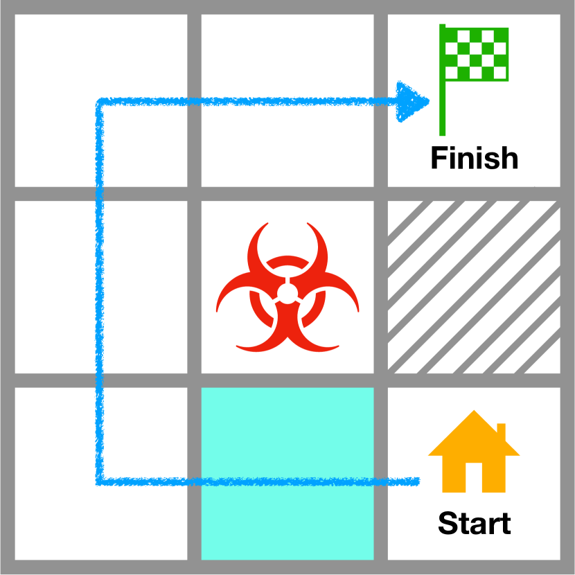
(b)

Figure 1: A simple 3x3 grid-world problem with two modes and the optimal path visualized in blue. (a) In the ‘No Trap’ mode, the center square is safe to pass through. (b) In the ‘Trap‘ mode, the agent needs to avoid the trap with a longer path.

Advantage Actor Critic (A2C).

We use the A2C algorithm to train a policy for this environment, while its context changes every so often. When in ‘No Trap’ mode, the closest path passes through the center cell, and the best episodic return is $-3$. In the ‘Trap Active’ mode, the center cell’s penalty is too high, and we must go left at the blue cell instead, to incur an optimal episodic return of $-5$. Figure 2(a) depicts the episodic return across time and Figure 2(b) depicts what fraction of the time the policy makes the correct decision to go up in the blue cell when the context is in ‘No Trap’ mode. As observed, the agent initially learns the correct decision for that cell when training in the ‘No Trap’ mode, but once the context (mode) changes at epoch 4K, it immediately forgets it. When the mode changes back to the initial ‘No Trap’ mode at epoch 16K, the agent behaves sub-optimally (epochs 16K-18K) before recovering.

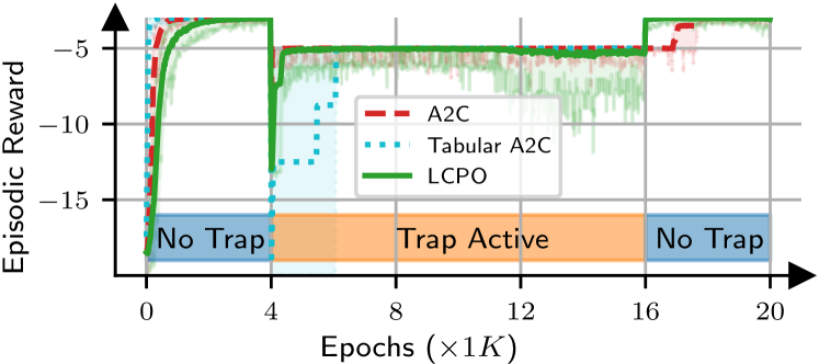
(a)

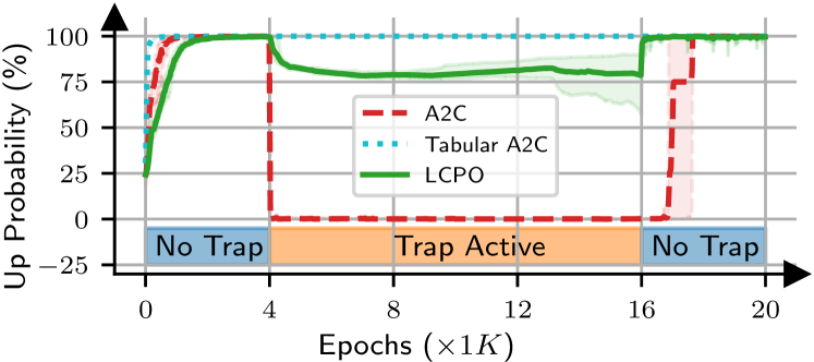
(b)

Figure 2: (a) Episodic return across time in the grid environment. (b) Probability of going up at the blue cell according to the policy, when at ‘No Trap’ mode. Note that in the ‘Trap Active’ period, the shown probability is not used in the episode, and only measures how much the agent has forgotten since epoch $4K$. LCPO remembers the optimal decision for ‘No Trap’ mode, even when it does not interact with that mode for 12K epochs, and instantly attains optimal returns at epoch 16K when the environment enters ‘No Trap’ mode again.

Key Insight.

Since the context $z_{t}$ is observed, the agent should be able to distinguish between different environment modes (even without an explicit task label). Therefore, if the agent could surgically modify its policy on the current state-context pairs $<s_{t},z_{t}>$ and leave all other state-context pairs unchanged, it would eventually learn a good policy for all contexts. In fact, tabular RL achieves this trivially in this finite discrete state-context space. To illustrate, we apply a tabular version of A2C: i.e., the policy and value networks are replaced with tables with separate rows for each state-context pair (18 total rows). As expected, in this case, the policy output, depicted in Figure 2(b), does not forget to go up in the blue cell in the ‘No Trap’ mode after epoch 4K. This is because when an experience is used to update the table, it only updates the row pertaining to its own state and context, and does not change rows belonging to other contexts.

Can we achieve a similar behavior with neural network function approximators? In general, updating a neural network (say, a policy network) for certain state-context pairs will change the output for all state-context pairs, leading to CF. But if we could somehow “anchor” the output of the neural network on distinct prior state-context pairs (analogous to the cells in the tabular setting) while we update the relevant state-context pairs, then the neural network would not “forget”.

LCPO.

Achieving the aforementioned anchoring does not require task labels. We only need to know if two contexts $z_{i}$ and $z_{j}$ are different. In particular, let the batch of recent environment interactions $<s_{t},z_{t},a_{t},r_{t}>$ be $B_{r}$ and let all previous interactions (from possibly different contexts) be $B_{a}$. Suppose we have a difference detector $W(B_{a},B_{r})$ that can be used to sample experiences from $B_{a}$ that are not from the same distribution as the samples in the recent batch $B_{r}$, i.e., the difference detector provides out-of-distribution (OOD) samples with respect to $B_{r}$. Then, when optimizing the policy for the current batch $B_{r}$, we can constrain the policy’s output on experiences sampled via $W(B_{a},B_{r})$ to not change (see §5 for details). We name this approach Locally Constrained Policy Optimization (LCPO). The result for LCPO is presented in Figure 2(b). While it does not retain its policy as perfectly as tabular A2C while in the ‘Trap Active’ mode, it does sufficiently well to recover near instantaneously upon the second switch at epoch 16K.

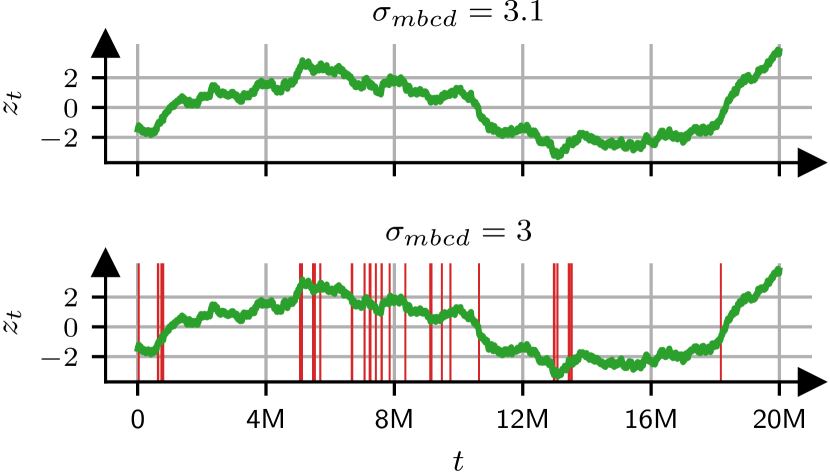
Figure 3: A sample context process $z_{t}$, and detected change-points for two thresholds. It is difficult to tease meaningful task boundaries from this process, but defining an OOD metric is intuitive.

Change-Point Detection (CPD) vs. OOD Detection.

CPD (and task labeling in general) requires stronger assumptions than OOD detection. The context process has to be piece-wise stationary to infer task labels and context changes must happen infrequently to be detectable. Furthermore, online CPD is sensitive to outliers. In contrast, OOD is akin to defining a distance metric on the context process and can be well-defined on any context process. Consider the context process shown in Figure 3. We run this context process through a CPD algorithm (Alegre et al., 2021) for two different sensitivity factors $\sigma_{mbcd}$, and represent each detected change-point with a red vertical line. Not only does a slight increase in sensitivity lead to 34 detected change-points, but these change-points are also not reasonable. There is no obvious way to assign task labels for this smooth process and there aren’t clearly separated segments that can be defined as tasks. However, an intuitive OOD detection method is testing if the distance between $z_{i}$ and $z_{j}$ is larger than some threshold, i.e., $|z_{i}-z_{j}|>\tau$. Altogether, OOD is considerably easier in practice compared to CPD. Note that although the grid-world example – and discrete context environments in general – is a good fit for CPD, this environment was purposefully simple to explain the insight behind LCPO.

5 Methodology

Consider a parameterized policy $\pi_{\theta}$ with parameters $\theta$. Our task is to choose a direction for changing $\theta$ such that it improves the expected return on the most recent batch of experiences $B_{r}$, while the policy is ‘anchored’ on prior samples with sufficiently distinct context distributions, $W(B_{a},B_{r})$.

In supervised learning, this anchoring is straightforward to perform, e.g. by adding a regularization loss that directs the neural network to output the ground truth labels for OOD samples (Caruana, 1997). In the case of an RL policy, however, we do not know the ground truth (optimal actions) for anchoring the policy output. Moreover, using the actions we took in prior contexts as the ground truth is not possible, since the policy may have not converged at those times. Anchoring to those actions may cause the policy to relearn suboptimal actions from an earlier period in training.

To avoid these problems, LCPO solves a constrained optimization problem that forces the policy to not change for OOD samples. Formally, we consider the following optimization problem:

$$\min_{\theta}~{}~{}\mathcal{L}_{tot}(\theta;B_{r})\triangleq\mathcal{L}_{PG}(\theta;B_{r}) +\mathcal{L}_{e}(\theta;B_{r})$$ (1)

$$s.t.~{}~{}D_{KL}(\theta_{0},\theta;W(B_{a},B_{r} ))\leq c_{anchor}$$

We use the standard definition of policy gradient loss, that optimizes a policy to maximize returns (Schulman et al., 2018; Mnih et al., 2016; Sutton & Barto, 2018):

$$\mathcal{L}_{PG}(\theta;B_{r})=\mathbb{E}_{r_{t}\sim B_{r}}\left[\sum_{t=0}^{H}-\gamma^{t}r_{t}\right]$$ (2)

We use automatic entropy regularization (Haarnoja et al., 2018c), to react to and explore in response to novel contexts. The learnable parameter $\theta_{e}$ is adapted such that the entropy coefficient is $e^{\theta_{e}}$, and the entropy remains close to a target entropy $\bar{\mathcal{H}}$. This worked well in our experiments but LCPO could use any exploration method designed for non-stationary context-driven environments.

$$\mathcal{L}_{e}(\theta;B_{r})=e^{\theta_{e}}.\left(\mathbb{E}_{s_{t},z_{t}\sim B_{r},a_{t}\sim\pi}\left[\log\pi(a_{t}|s_{t},z_{t})\right]\right)$$ (3)

We use KL-divergence as a measure of policy change, and for simplicity we use $D_{KL}(\theta_{0},\theta;W(B_{a},B_{r}))$ as a shorthand for $\mathbb{E}_{s,z\sim W(B_{a},B_{r})}[D_{KL}(\pi_{\theta_{0}}(s,z)||\pi_{\theta}(s,z))]$. Here, $\theta_{0}$ denotes the current policy parameters, and we are solving the optimization over $\theta$ to determine the new policy parameters.

Algorithm 1 LCPO Training

1:  initialize parameter vectors $\theta_{0}$, empty buffer $B_{a}$

2:  for each iteration do

3:     $B_{r}\leftarrow$ Sample a mini-batch of new interactions

4:     $S_{c}\leftarrow W(B_{a},B_{r})$

5:     $v\leftarrow\nabla_{\theta}\mathcal{L}_{tot}(\theta;B_{r})|_{\theta_{0}}$

6:     if $S_{c}$ is not empty then

7:        $g(x):=\nabla_{\theta}(x^{T}\nabla_{\theta}\mathcal{D}_{KL}(\theta,\theta_{old};S_{c})|_{\theta_{0}})|_{\theta_{0}}$

8:        $v_{c}\leftarrow conjgrad(v,g(\cdot))$

9:        while $\theta_{old}+v_{c}$ violates constraints do

10:           $v_{c}\leftarrow v_{c}/2$

11:        end while

12:        $\theta_{0}\leftarrow\theta_{0}+v_{c}$

13:     else

14:        $\theta_{0}\leftarrow\theta_{0}+v_{tot}$

15:     end if

16:     $B_{a}\leftarrow B_{a}+B_{r}$

17:  end for

Buffer Management.

To avoid storing all interactions in $B_{a}$ we use reservoir sampling (Vitter, 1985), where we randomly replace old interactions with new ones with probability $\frac{n_{b}}{n_{s}}$, where $n_{b}$ is the buffer size and $n_{s}$ is the total interactions thus far. Reservoir sampling guarantees that the interactions in the buffer are a uniformly random subset of the full set of interactions.

Difference detector.

To realize $W(B_{a},B_{r})$, we treat it as an out-of-distribution detection (OOD) task. A variety of methods can be used for this in practice (§6). For example, we can compute the Mahalanobis distance (Mahalanobis, 2018), i.e. the normalized distance of each experience’s context, with respect to the average context in $B_{r}$, and deem any distance above a certain threshold to be OOD. To avoid a high computational overhead when sampling from $W(B_{a},B_{r})$, we sample a mini-batch from $B_{a}$, and keep the state-context pairs that are OOD with respect to $B_{r}$. We repeat this step up to five times. If not enough different samples exist, we do not apply the constraint for that update.

Solving the constrained optimization.

To solve this constrained optimization, we approximate the optimization goal and constraint, and calculate a search direction accordingly (pseudocode in Algorithm 1). Our problem is structurally similar to TRPO (Schulman et al., 2015), though the constraint is quite different. Similar to TRPO, we model the optimization goal with a first-order approximation, i.e. $\mathcal{L}_{tot}(\theta;\cdot)=\mathcal{L}_{0}+(\theta-\theta_{0})^{T}\nabla_{\theta}\mathcal{L}_{tot}(\theta;\cdot)|_{\theta_{0}}$, and the constraint with a second order approximation $D_{KL}(\theta,\theta_{0};\cdot)=(\theta-\theta_{0})^{T}\nabla^{2}_{\theta}D_{KL}(\theta,\theta_{0};\cdot)|_{\theta_{0}}(\theta-\theta_{0})$. The optimization problem can therefore be written as:

$$\min_{\theta}~{}~{}(\theta-\theta_{0})^{T} v$$ (4)

$$s.t.~{}~{}(\theta-\theta_{0})^{T}A(\theta- \theta_{0})\leq c_{anchor}$$

where $A_{ij}=\frac{\partial}{\partial\theta_{i}}{\frac{\partial}{\partial\theta_{j}}}D_{KL}(\theta,\theta_{0};W(B_{a},B_{r}))$, and $v=\nabla_{\theta}\mathcal{L}_{tot}(\theta;\cdot)|_{\theta_{0}}$. This optimization problem can be solved using the conjugate gradient method followed by a line search as described in TRPO (Schulman et al., 2015).

Bounding policy change.

The above formulation does not bound policy change on the current context, which could destabilize learning. We could add a second constraint, i.e. TRPO’s constraint, $D_{KL}(\theta_{0},\theta;B_{r})\leq c_{recent}$, but having two second order constraints is computationally expensive. Instead, we guarantee the TRPO constraint in the line search phase (lines 9–10 in Algorithm 1), where we repeatedly decrease the gradient update size until both constraints are met.

6 Evaluation

We evaluate LCPO across six environments: four from Gymnasium Mujoco (Towers et al., 2023), one from Gymnasium Classic Control (Towers et al., 2023), and a straggler mitigation task from computer systems (Hamadanian et al., 2022). These environments are subject to synthetic or real context processes that affect their dynamics. Our experiments aim to answer the following questions: (1) How does LCPO compare to state-of-the-art on-policy, off-policy, model-based baselines and pre-trained oracle policies (§6.1)? (2) How does the maximum buffer size $n_{b}=|B_{a}|$ affect LCPO (§6.2)? (3) How does the accuracy of the OOD sampler $W(\cdot,\cdot)$ affect LCPO (§6.3)?

Baselines.

We consider the following approaches. (1) Model-Based Changepoint Detection (MBCD) (Alegre et al., 2021): This approach is the state-of-the-art technique for handling piece-wise stationary environments without task labels. It trains models to predict environment state transitions, and launches new policies when the current model is inaccurate in predicting the state trajectory. The underlying learning approach is Soft Actor Critic (SAC) (Haarnoja et al., 2018b). (2) Model-Based Policy Optimization (MBPO) (Janner et al., 2021): A model-based approach that trains an ensemble of experts to learn the environment model, and generates samples for an SAC (Haarnoja et al., 2018b) algorithm. If the model is accurate, it can fully replay prior contexts, thereby avoiding catastrophic forgetting. (3) Online Elastic Weight Consolidation (EWC) (Chaudhry et al., 2018; Schwarz et al., 2018): EWC regularizes online learning with a Bayesian approach assuming task indices, and online EWC generalizes it to task boundaries. To adapt online EWC to our problem, we update the importance vector and average weights using a weighted moving average in every time step. The underlying learning approach is SAC (Haarnoja et al., 2018b). (4) On-policy RL: On-policy RL is susceptible to CF, but more stable in online learning compared to off-policy RL algorithms. We compare with A2C (Mnih et al., 2016) and TRPO (single-path) (Schulman et al., 2015), with Generalized Advantage Estimation (GAE) (Schulman et al., 2018) applied. Note that TRPO vine is not possible in online learning, as it requires rolling back the environment world. (5) Off-policy RL: Off-policy RL is potentially capable of overcoming CF due to replay buffers, at the cost of unstable training. We consider Double Deep Q Network (DDQN) (Hasselt et al., 2016) and SAC (with automatic entropy regularization, similar to LCPO) (Haarnoja et al., 2018b). (6) Oracle RL: To establish an upper-bound on the best performance that an online learner can achieve, we train oracle policies. We allow oracle policies to have unlimited access to the contexts and environment dynamics, i.e. they are able to replay any particular environment and context as many times as necessary. Since oracle policies can interact with multiple contexts in parallel during training, they do not suffer from CF. In contrast, all other baselines (and LCPO) are only allowed to experience contexts sequentially as they occur over time and must adapt the policy on the go. We report results for the best of four oracle policies with the following model-free algorithms: A2C (Mnih et al., 2016), TRPO (single-path) (Schulman et al., 2015), DDQN (Hasselt et al., 2016) and SAC (Haarnoja et al., 2018b).

Experiment Setup.

We use 5 random seeds for gymnasium and 10 random seeds for the straggler mitigation experiments, and use the same hyperparameters for LCPO in all environments and contexts. Hyperparameters and neural network structures are noted in Appendices §A.4 and §B.2. These experiments were conducted on a machine with 2 AMD EPYC 7763 CPUs (256 logical cores) and 512 GiB of RAM. With 32 concurrent processes, the experiments finished in $\sim$364 hours.

Environment and Contexts.

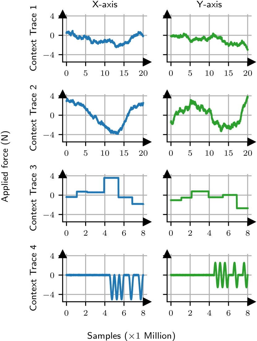
Figure 7: External wind force, per axis and context trace.

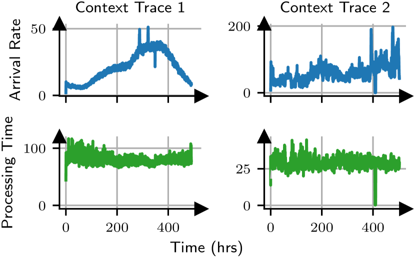
Figure 9: Request arrival rate and processing time per context.

We consider six environments: Modified versions of Pendulum-v1 from the classic control environments, InvertedPendulum-v4, InvertedDoublePendulum-v4, Hopper-v4 and Reacher-v4 from the Mujoco environments (Towers et al., 2023), and a straggler mitigation environment (Hamadanian et al., 2022). In the gym environments, the context is an exogenous “wind” process that creates external force on joints and affects movements. We append the external wind vectors from the last 3 time-steps to the observation, since the agent cannot observe the external context that is going to be applied in the next step, and a history of prior steps helps with the prediction. We create 4 synthetic context sequences with the Ornstein–Uhlenbeck process (Uhlenbeck & Ornstein, 1930), piece-wise Gaussian models, or hand-crafted signals with additive noise. These context processes cover smooth, sudden, stochastic, and predictable transitions at short horizons. All context traces are visualized in Figure 7 in the appendix. For the straggler mitigation environments, we use workloads provided by the authors in (Hamadanian et al., 2022), that are from a production web framework cluster at AnonCo, collected from a single day in February 2018. These workloads are visualized in Figure 9 in the appendix.

OOD detection.

We set the buffer size $n_{b}$ to 1% of all samples, which is $n_{b}\leq 200K$. To sample OOD state-context pairs $W(B_{a},B_{r})$, we use distance metrics and thresholds. For gym environments where the context is a wind process, we use L2 distance, i.e. if $\overline{w_{r}}=\mathbb{E}_{w\sim B_{r}}[w]$ is the average wind vector observed in the recent batch $B_{r}$, we sample a minibatch of states in $B_{a}$ where $W(B_{a},B_{r})=\{w_{i}|\forall w_{i}\in B_{a}:\lVert w_{i}-\overline{w_{r}}\rVert_{2}>\sigma\}$. There exist domain-specific models for workload distributions in the straggler mitigation environment, but we used Mahalanobis distance as it is a well-accepted and general approach for outlier detection in prior work (Lee et al., 2018; Podolskiy et al., 2021). Concretely, we fit a Gaussian multivariate model to the recent batch $B_{r}$, and report a minibatch of states in $B_{a}$ with a Mahalanobis distance further than $\sigma$ from this distribution.

6.1 Results

Results.

To evaluate across gymnasium environments, we score online learning baselines with Normalized Return, i.e., a scaled score function where 0 and 1 are the minimum and maximum return across all agents. Figure 4 provides a summary of all gymnasium experiments (for full details refer to Table 2 in the Appendix). LCPO maintains a lead over baselines, is close to the best-performing oracle policy, all while learning online and sequentially. MBCD struggles to tease out meaningful task boundaries. In some experiments, it launches anywhere between 3 to 7 policies just by changing the random seed. This observation is in line with MBCD’s sensitivity in §4.

MBPO performed poorly, even though we verified that its learned model of the environment is highly accurate. The reason is the way that MBPO samples experiences for training. At every iteration, MBPO samples a batch of actual interactions from its experience buffer and generates hypothetical interactions from them. These hypothetical interactions amass in a second buffer, which is used to train an SAC agent. During the course of training, the second buffer accumulates more interactions generated from samples from the start of the experiment compared to recent samples. This is not an issue when the problem is stationary, but in non-stationary RL subject to an context process, this leads to over-emphasis of the context processes encountered earlier in the experiment. As such, MBPO fails to even surpass SAC. Prior work has observed the sensitivity of off-policy approaches to such sampling strategies (Isele & Cosgun, 2018; Hamadanian et al., 2022). In our experiments, we also observe that the on-policy A2C usually outperforms the off-policy SAC and Deep Q Network (DQN).

Table 1: Tail latency (negative reward) and 95th percentile confidence ranges for different algorithms and contexts in the straggler mitigation environment.

	Online Learning
	LCPO	LCPO	LCPO	MBCD	MBPO	Online EWC	A2C	TRPO	DDQN	SAC	Best
	Agg	Med	Cons								Oracle
Workload 1	1070	1076	1048	1701	2531	2711	1716	3154	1701	1854	984
	$\pm$10	$\pm$16	$\pm$7	$\pm$112	$\pm$197	$\pm$232	$\pm$710	$\pm$464	$\pm$47	$\pm$245	(TRPO)
Workload 2	589	617	586	678	891	724	604	864	633	644	509
	$\pm$43	$\pm$62	$\pm$27	$\pm$38	$\pm$54	$\pm$22	$\pm$109	$\pm$105	$\pm$7	$\pm$27	(A2C)

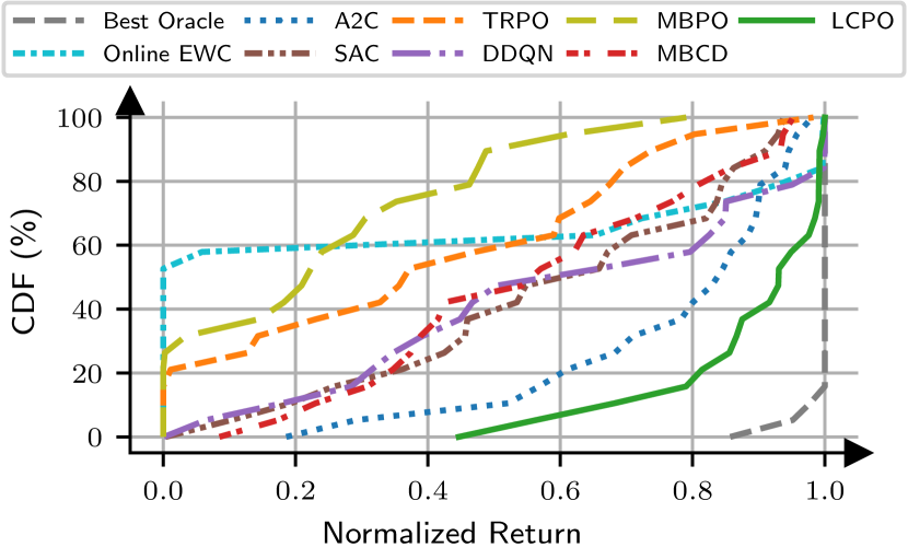
Figure 4: Normalized episodic returns, where 0 and 1 denote the lowest and highest returns among agents. LCPO outperforms all online agents, and remains the closest to oracles.

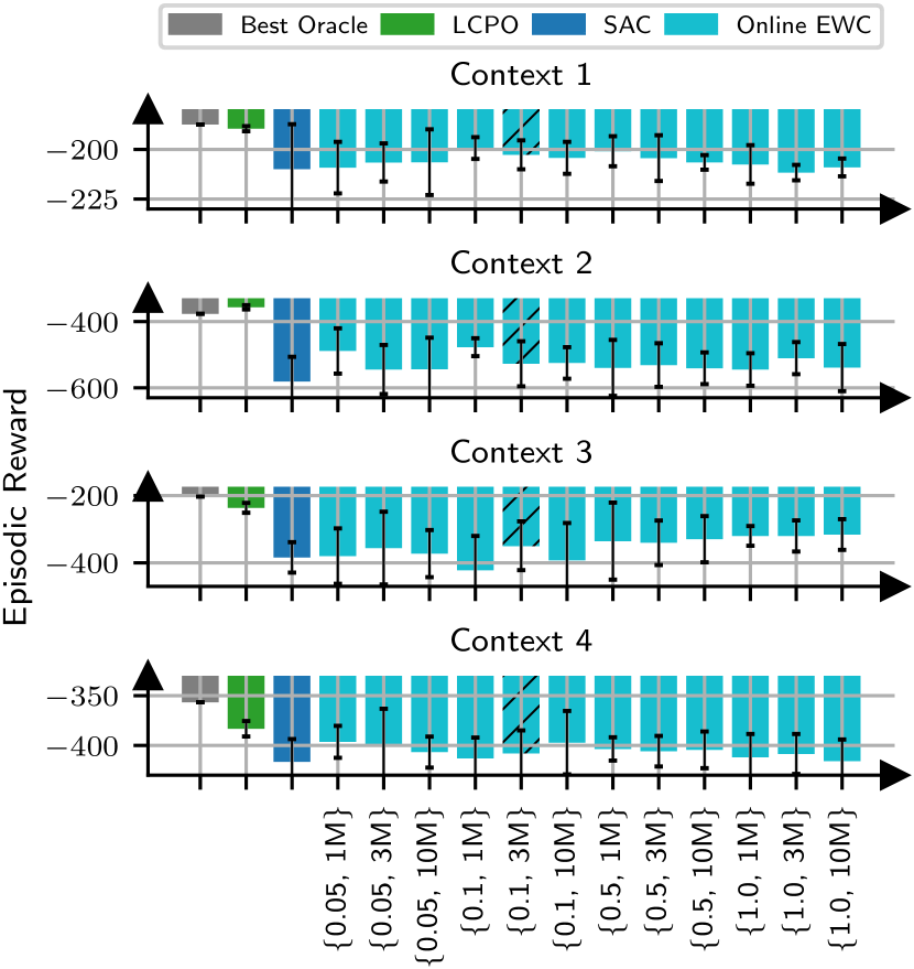
Figure 5: Pendulum-v1 episodic returns and 95% confidence bounds of Online EWC with 12 hyperparameter trials. Hyperparameters are labeled as $\{\alpha,\beta^{-1}\}$, where $\alpha$ is the regularization strength and $\beta$ is the averaging weight. The optimal online EWC hyperparameter is sensitive to the context, but LCPO is better even if online EWC is tuned per context.

Online EWC applies a regularization loss $\mathcal{L}_{ewc}=\alpha\lvert\lvert\theta_{t}-\theta_{t-1}^{*}\rvert\rvert^{2}_{F_{t-1}^{*}}$ to the training loss, using a running average $F_{t}^{*}$ of the diagonal of the Fisher Information Matrix (FIM), and a running average of the parameters $\theta_{t}^{*}$. The running average $F_{t}^{*}$ is updated with a weighted average $F_{t}^{*}=(1-\beta)F_{t-1}^{*}+\beta F_{t}$, where $F_{t}$ is the diagonal of the FIM respective to the recent parameters and samples. Similarly, the running average $\theta_{t}^{*}$ uses the same parameter $\beta$.

Online EWC may constrain the policy output to remain constant on samples in the last $\approx\beta^{-1}$ epochs, but it has to strike a balance between how fast the importance metrics are updated with the newest FIM (larger $\beta$) and how long the policy has to remember its training (smaller $\beta$). This balance will ultimately depend on the context trace and how frequently they evolve. We tuned $\alpha$ and $\beta$ on Pendulum-v1 for all contexts, trying $\alpha\in\{0.05,0.1,0.5,1.0,10,100,1000\}$ and $\beta^{-1}\in\{1M,3M,10M\}$. The returns are visualized in Figure 5 (with full details in Table 4 in the Appendix). There is no universal $\beta$ that works well across all contexts and online EWC would not perform better than LCPO even if tuned to each context trace individually. We ultimately chose $\beta^{-1}=3M$ samples to strike a balance across all contexts, but it struggled to even surpass SAC on other environments.

For the straggler mitigation environment, Table 1 presents the latency metric (negative reward) over two workloads. Recall that this environment uses real-world traces from a production cloud network. The overall trends are similar to the gymnasium experiments, with LCPO outperforming all other baselines. This table includes three variants of LCPO, that will be discussed further in §6.3.

6.2 Sensitivity to Buffer Size

LCPO uses Reservoir sampling (Vitter, 1985) to maintain a limited number of samples $n_{b}$. We evaluate how sensitive LCPO is to the buffer size in Figure 6 (full results in Table 3 in the Appendix). The full experiment has 8–20M samples. LCPO maintains its high performance, even with as little as $n_{b}=500$ samples, but drops below this point. This is not surprising, as the context traces do not change drastically at short intervals, and even 500 randomly sampled points from the trace should be enough to have a representation over all the trace. However, it is likely that with more complicated and high-dimensional contexts, a higher buffer size would be necessary.

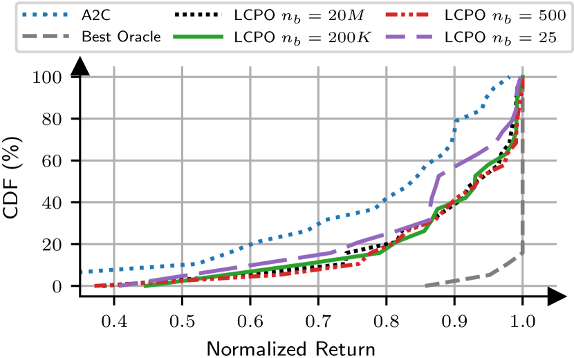
Figure 6: Normalized returns of LCPO in gymnasium environments with various buffer sizes. LCPO loses performance with $n_{b}<500$.

6.3 Sensitivity to OOD metric

LCPO applies a constraint to OOD state-context pairs, as dictated by the OOD sampler $W(B_{a},B_{r})$. We vary the Mahalanobis distance threshold $\sigma$, the threshold that the OOD method uses in sampling, and monitor the normalized return for the straggler mitigation environment. LCPO Agg, LCPO Med and LCPO Cons use $\sigma=5$, $6$ and $7$, and a higher value for $\sigma$ yields more conservative OOD samples (i.e., fewer samples are detected as OOD). The difference between these three is significant: The model in LCPO Agg allows for $26.7\times$ more samples to be considered OOD compared to LCPO Cons. Table 1 provides the normalized return for LCPO with varying thresholds, along with baselines. Notably, all variations of LCPO achieve similar results.

7 Discussion and Limitations

Network Capacity.

In general, online learning methods with bounded parameter counts will reach the function approximator’s (neural network’s) maximum representational capacity. LCPO is not immune from this, as we do not add parameters with more context traces. However, neither are oracle agents. To isolate the effect of this capacity and CF, we compare against oracle agents, rather than single agents trained on individual tasks or context traces (He et al., 2020). This ensures a fair evaluation that does not penalize online learning for reaching the capacity ceiling.

Exploration.

LCPO focuses on mitigating catastrophic forgetting in non-stationary RL. An orthogonal challenge in this setting is efficient exploration, i.e. to explore when the context distribution has changed but only once per new context. Our experiments used automatic entropy tuning for exploration (Haarnoja et al., 2018b). While empirically effective, this approach was not designed for non-stationary problems, and LCPO may benefit from a better exploration methodology such as curiosity-driven exploration (Pathak et al., 2017).

Efficient Buffer Management.

We used Reservoir Sampling (Vitter, 1985), which maintains a uniformly random buffer of all observed state-context samples so far. Future work could explore more efficient strategies that selectively store or drop samples based on their context, e.g., to maximize sample diversity.

8 Conclusion

We proposed and evaluated LCPO, a simple approach for learning policies in non-stationary context-driven environments. Using LCPO requires two conditions: (1) the non-stationarity must be induced by an exogenous observed context process; and (2) a similarity metric is required that can inform us if two contexts come from noticeably different distributions (OOD detection). This is less restrictive than prior approaches that require either explicit or inferred task labels. Our experiments showed that LCPO outperforms state-of-the-art baselines on several environments with real and synthetic context processes.

9 Broader Impact

Our work advances the field of reinforcement learning. Online learning in non-stationary environments is an important hurdle for deploying RL agents in the real world. There are many potential societal consequences, none which we feel must be specifically highlighted here.

Appendix A Locomotion tasks in Gymnasium

A.1 Full results

Table 2 presents the episodic return for all agents, environments and context traces. Table 3 presents the episodic return for multiple LCPO agents with different buffer sizes $n_{b}$. Table 4 presents the episodic return for online EWC agents with various hyperparameter values in the Pendulum-v1 environment.

Table 2: Average and 95th percentile confidence ranges for episodic return for different algorithms and conditions in environments with external wind processes.

		Online Learning									Oracle Policies
		LCPO	Online EWC	MBCD	MBPO	A2C	TRPO	DDQN	SAC		A2C	TRPO	DDQN	SAC
Pendulum	Context Trace 1	-190	-197	-207	-325	-203	-224	-216	-210		-208	-197	-188	-187
		$\pm$1.29	$\pm$7.63	$\pm$23.4	$\pm$47.2	$\pm$10.2	$\pm$11.2	$\pm$16.9	$\pm$22.7
	Context Trace 2	-357	-523	-577	-843	-373	-512	-755	-581		-407	-399	-376	-380
		$\pm$6.38	$\pm$58.8	$\pm$71.3	$\pm$24.2	$\pm$24.2	$\pm$45.1	$\pm$369	$\pm$74.2
	Context Trace 3	-237	-314	-349	-603	-330	-511	-577	-384		-224	-320	-228	-203
		$\pm$14.6	$\pm$45.8	$\pm$28.9	$\pm$213	$\pm$111	$\pm$205	$\pm$194	$\pm$45.2
	Context Trace 4	-383	-415	-430	-553	-395	-741	-414	-416		-383	-381	-384	-357
		$\pm$7.73	$\pm$22.0	$\pm$15.4	$\pm$90.9	$\pm$14.0	$\pm$137	$\pm$27.2	$\pm$22.8
Inverse Pendulum	Context Trace 1	18.2	3.45	6.17	2.88	6.46	2.07	14.0	4.50		24.4	25.7	24.1	24.8
		$\pm$12.3	$\pm$1.47	$\pm$6.10	$\pm$1.78	$\pm$8.35	$\pm$0.34	$\pm$5.11	$\pm$3.66
	Context Trace 2	4.63	1.50	2.10	1.52	3.54	2.39	1.51	1.53		7.86	8.51	7.18	7.75
		$\pm$2.20	$\pm$0.08	$\pm$1.06	$\pm$0.01	$\pm$2.38	$\pm$1.95	$\pm$0.07	$\pm$0.01
	Context Trace 3	15.1	6.36	14.2	14.4	14.5	7.81	15.0	14.7		15.5	16.5	15.1	14.3
		$\pm$0.87	$\pm$3.12	$\pm$0.77	$\pm$0.23	$\pm$2.11	$\pm$8.63	$\pm$0.56	$\pm$0.16
	Context Trace 4	92.2	4.78	46.5	37.6	93.7	79.5	93.3	53.8		102	112	53.7	40.1
		$\pm$0.48	$\pm$1.15	$\pm$4.85	$\pm$0.98	$\pm$0.71	$\pm$32.4	$\pm$1.80	$\pm$6.09
Inverse Double Pendulum	Context Trace 1	110	38.2	77.3	68.5	110	79.7	82.2	83.8		142	165	88.0	95.5
		$\pm$5.84	$\pm$5.46	$\pm$13.5	$\pm$19.3	$\pm$15.6	$\pm$60.1	$\pm$3.17	$\pm$2.94
	Context Trace 2	59.8	30.1	44.2	37.2	54.2	30.5	40.8	36.7		51.4	64.0	46.8	49.5
		$\pm$5.03	$\pm$1.35	$\pm$3.27	$\pm$9.92	$\pm$4.25	$\pm$14.8	$\pm$5.48	$\pm$7.03
	Context Trace 3	66.3	37.4	45.8	42.7	59.7	54.6	61.4	46.8		63.5	74.0	63.6	47.4
		$\pm$2.47	$\pm$2.88	$\pm$2.38	$\pm$1.55	$\pm$11.4	$\pm$5.87	$\pm$0.52	$\pm$0.39
	Context Trace 4	88.6	39.1	75.0	59.5	88.0	76.4	94.1	80.0		91.9	96.9	90.7	78.0
		$\pm$1.55	$\pm$12.6	$\pm$4.65	$\pm$2.86	$\pm$1.87	$\pm$6.16	$\pm$0.52	$\pm$0.68
Hopper	Context Trace 1	245	31.4	153	130	199	157	131	172		240	215	155	184
		$\pm$24.0	$\pm$21.6	$\pm$33.2	$\pm$12.8	$\pm$10.3	$\pm$31.0	$\pm$27.6	$\pm$8.75
	Context Trace 2	142	33.1	76.0	66.0	92.9	74.0	65.7	81.8		128	131	86.6	96.7
		$\pm$14.2	$\pm$19.0	$\pm$15.3	$\pm$18.2	$\pm$10.3	$\pm$12.7	$\pm$17.5	$\pm$14.0
	Context Trace 3	508	32.0	240	264	469	424	224	256		520	492	327	308
		$\pm$10.4	$\pm$39.8	$\pm$81.7	$\pm$49.9	$\pm$73.5	$\pm$67.5	$\pm$9.42	$\pm$125
	Context Trace 4	298	25.3	127	205	277	201	157	223		319	297	189	189
		$\pm$11.0	$\pm$18.2	$\pm$27.3	$\pm$37.5	$\pm$2.47	$\pm$74.7	$\pm$17.9	$\pm$66.9
Reacher	Context Trace 1	-26.8	-15.8	-169	-1862	-138	-2394	-7.86	-224		-8.00	-7.59	-7.59	-14.3
		$\pm$0.80	$\pm$1.63	$\pm$122	$\pm$2255	$\pm$136	$\pm$1266	$\pm$0.11	$\pm$412
	Context Trace 2	-20.0	-16.2	-339	-4308	-108	-5267	-7.78	-733		-8.33	-3866	-7.41	-15.3
		$\pm$0.32	$\pm$0.79	$\pm$493	$\pm$3764	$\pm$130	$\pm$1190	$\pm$0.18	$\pm$1591
	Context Trace 3	-27.5	-15.4	-596	-2058	-208	-43.9	-8.60	-137		-9.63	-8.42	-8.41	-15.7
		$\pm$2.40	$\pm$0.19	$\pm$857	$\pm$4173	$\pm$400	$\pm$51.6	$\pm$0.20	$\pm$212
	Context Trace 4	-29.3	-16.3	-121	-2354	-149	-1482	-11.9	-174		-9.63	-8.57	-7.97	-15.7
		$\pm$1.04	$\pm$1.20	$\pm$161	$\pm$2988	$\pm$227	$\pm$639	$\pm$7.37	$\pm$353

Table 3: Average and 95th percentile confidence ranges for episodic return in LCPO with multiple buffer sizes and other agents for different conditions in environments with external wind processes.

		Online Learning
		LCPO 20M	LCPO 200K	LCPO 500	LCPO 25	Online EWC	MBCD	MBPO	A2C		Best Oracle
Pendulum	Context Trace 1	-190	-190	-191	-193	-197	-207	-325	-203		-187
		$\pm$2.39	$\pm$1.29	$\pm$4.95	$\pm$2.67	$\pm$7.63	$\pm$23.4	$\pm$47.2	$\pm$10.2		(SAC)
	Context Trace 2	-361	-357	-353	-360	-523	-577	-843	-373		-376
		$\pm$6.16	$\pm$6.38	$\pm$5.07	$\pm$15.5	$\pm$58.8	$\pm$71.3	$\pm$24.2	$\pm$24.2		(DDQN)
	Context Trace 3	-238	-237	-232	-256	-314	-349	-603	-330		-203
		$\pm$17.7	$\pm$14.6	$\pm$22.3	$\pm$23.4	$\pm$45.8	$\pm$28.9	$\pm$213	$\pm$111		(SAC)
	Context Trace 4	-378	-383	-380	-404	-415	-430	-553	-395		-357
		$\pm$8.09	$\pm$7.73	$\pm$16.3	$\pm$7.74	$\pm$22.0	$\pm$15.4	$\pm$90.9	$\pm$14.0		(SAC)
Inverse Pendulum	Context Trace 1	21.5	18.2	21.7	14.1	3.45	6.17	2.88	6.46		25.7
		$\pm$1.69	$\pm$12.3	$\pm$2.18	$\pm$11.5	$\pm$1.47	$\pm$6.10	$\pm$1.78	$\pm$8.35		(TRPO)
	Context Trace 2	4.19	4.63	4.10	4.35	1.50	2.10	1.52	3.54		8.51
		$\pm$2.95	$\pm$2.20	$\pm$2.66	$\pm$3.26	$\pm$0.08	$\pm$1.06	$\pm$0.01	$\pm$2.38		(TRPO)
	Context Trace 3	15.4	15.1	15.3	15.5	6.36	14.2	14.4	14.5		16.5
		$\pm$0.83	$\pm$0.87	$\pm$0.78	$\pm$0.22	$\pm$3.12	$\pm$0.77	$\pm$0.23	$\pm$2.11		(TRPO)
	Context Trace 4	92.2	92.2	92.1	92.3	4.78	46.5	37.6	93.7		112
		$\pm$0.76	$\pm$0.48	$\pm$0.61	$\pm$0.55	$\pm$1.15	$\pm$4.85	$\pm$0.98	$\pm$0.71		(TRPO)
Inverse Double Pendulum	Context Trace 1	113	110	119	116	38.2	77.3	68.5	110		165
		$\pm$4.16	$\pm$5.84	$\pm$32.7	$\pm$12.4	$\pm$5.46	$\pm$13.5	$\pm$19.3	$\pm$15.6		(TRPO)
	Context Trace 2	55.3	59.8	56.5	54.5	30.1	44.2	37.2	54.2		64.0
		$\pm$3.82	$\pm$5.03	$\pm$7.47	$\pm$4.35	$\pm$1.35	$\pm$3.27	$\pm$9.92	$\pm$4.25		(TRPO)
	Context Trace 3	64.5	66.3	65.2	65.2	37.4	45.8	42.7	59.7		74.0
		$\pm$2.18	$\pm$2.47	$\pm$2.01	$\pm$2.77	$\pm$2.88	$\pm$2.38	$\pm$1.55	$\pm$11.4		(TRPO)
	Context Trace 4	89.2	88.6	89.5	89.5	39.1	75.0	59.5	88.0		96.9
		$\pm$0.36	$\pm$1.55	$\pm$0.57	$\pm$0.19	$\pm$12.6	$\pm$4.65	$\pm$2.86	$\pm$1.87		(TRPO)
Hopper	Context Trace 1	242	245	244	231	31.4	153	130	199		240
		$\pm$19.4	$\pm$24.0	$\pm$12.0	$\pm$7.57	$\pm$21.6	$\pm$33.2	$\pm$12.8	$\pm$10.3		(A2C)
	Context Trace 2	144	142	148	132	33.1	76.0	66.0	92.9		131
		$\pm$10.9	$\pm$14.2	$\pm$7.73	$\pm$13.8	$\pm$19.0	$\pm$15.3	$\pm$18.2	$\pm$10.3		(TRPO)
	Context Trace 3	505	508	509	506	32.0	240	264	469		520
		$\pm$5.12	$\pm$10.4	$\pm$8.82	$\pm$5.77	$\pm$39.8	$\pm$81.7	$\pm$49.9	$\pm$73.5		(A2C)
	Context Trace 4	295	298	290	279	25.3	127	205	277		319
		$\pm$13.4	$\pm$11.0	$\pm$6.15	$\pm$11.0	$\pm$18.2	$\pm$27.3	$\pm$37.5	$\pm$2.47		(A2C)
Reacher	Context Trace 1	-26.6	-26.8	-26.8	-26.3	-15.8	-169	-1862	-138		-7.59
		$\pm$0.38	$\pm$0.80	$\pm$0.54	$\pm$0.25	$\pm$1.63	$\pm$122	$\pm$2255	$\pm$136		(DDQN)
	Context Trace 2	-20.0	-20.0	-20.0	-19.9	-16.2	-339	-4308	-108		-7.41
		$\pm$0.37	$\pm$0.32	$\pm$0.37	$\pm$0.38	$\pm$0.79	$\pm$493	$\pm$3764	$\pm$130		(DDQN)
	Context Trace 3	-28.4	-27.5	-28.2	-28.3	-15.4	-596	-2058	-208		-8.41
		$\pm$1.05	$\pm$2.40	$\pm$1.46	$\pm$0.50	$\pm$0.19	$\pm$857	$\pm$4173	$\pm$400		(DDQN)
	Context Trace 4	-29.5	-29.3	-29.5	-29.4	-16.3	-121	-2354	-149		-7.97
		$\pm$0.87	$\pm$1.04	$\pm$2.56	$\pm$2.76	$\pm$1.20	$\pm$161	$\pm$2988	$\pm$227		(DDQN)

Table 4: Average and 95th percentile confidence ranges for episodic returns for online EWC variants in the Pendulum-v1 environment with external wind processes.

	Online EWC
	$\alpha=0.05$				$\alpha=0.1$				$\alpha=0.5$				$\alpha=1.0$
$\beta^{-1}\times$ rollout length:	$1M$	$3M$	$10M$		$1M$	$3M$	$10M$		$1M$	$3M$	$10M$		$1M$	$3M$	$10M$
Context Trace 1	-209	-207	-206		-199	-203	-204		-201	-204	-207		-208	-212	-209
	$\pm$13.0	$\pm$9.59	$\pm$16.6		$\pm$5.47	$\pm$7.28	$\pm$8.06		$\pm$7.57	$\pm$11.5	$\pm$3.67		$\pm$9.69	$\pm$3.87	$\pm$4.49
Context Trace 2	-489	-545	-544		-477	-527	-525		-540	-531	-541		-545	-510	-539
	$\pm$68.6	$\pm$74.1	$\pm$95.3		$\pm$26.9	$\pm$67.9	$\pm$47.6		$\pm$84.6	$\pm$65.9	$\pm$48.0		$\pm$49.0	$\pm$48.5	$\pm$71.2
Context Trace 3	-380	-356	-372		-422	-349	-393		-335	-340	-330		-320	-320	-316
	$\pm$82.4	$\pm$108	$\pm$70.0		$\pm$102	$\pm$72.4	$\pm$111		$\pm$114	$\pm$66.1	$\pm$68.5		$\pm$29.1	$\pm$46.1	$\pm$45.7
Context Trace 4	-396	-400	-407		-413	-408	-397		-404	-406	-404		-412	-409	-416
	$\pm$16.1	$\pm$36.7	$\pm$15.6		$\pm$21.1	$\pm$23.0	$\pm$31.9		$\pm$11.7	$\pm$15.4	$\pm$18.5		$\pm$23.5	$\pm$20.1	$\pm$21.7

A.2 MBPO with ground truth models

MBPO did not perform well in our online experiments. If the fault is the accuracy of the learned environment models, it could be improved with approaches such online meta-learning (Finn et al., 2019). We investigated the learned models for the Pendulum-v1 experiments manually. We found these models to be very accurate, since the environment dynamics are simple. As stated in §6.1, MBPO’s fails to address CF due to the way it samples data for training its policies.

To concretely verify that the accuracy of MBPO learned models is not the reason it underperforms, we instantiated an MBPO agent with access to the ground truth environment dynamics and context traces, which we call Ideal MBPO. We compare the performance of Ideal MBPO vs. standard MBPO in Table 5. The performance of these two agents is widely similar. This confirms the fact that the learning algorithm itself is the problem, and not the learned models.

Table 5: Average and 95th percentile confidence ranges for episodic returns for different algorithms and conditions in the Pendulum-v1 environment with external wind processes. An MBPO agent with access to the ground truth model performs similarly to the MBPO model.

	Online Learning
	LCPO	MBPO	Ideal MBPO	A2C	Best Oracle
Context Trace 1	-190	-325	-320	-203	-187 (SAC)
	$\pm$1.29	$\pm$47.2	$\pm$44.2	$\pm$10.2
Context Trace 2	-357	-843	-870	-373	-376 (DDQN)
	$\pm$6.38	$\pm$24.2	$\pm$56.4	$\pm$24.2
Context Trace 3	-237	-603	-637	-330	-203 (SAC)
	$\pm$14.6	$\pm$213	$\pm$90.0	$\pm$111
Context Trace 4	-383	-553	-555	-395	-357 (SAC)
	$\pm$7.73	$\pm$90.9	$\pm$84.1	$\pm$14.0

A.3 Action Space

Pendulum-v1 (and Mujoco environments) by default have continuous action spaces, ranging from $-2$ to $2$ for Pendulum-v1. We observed instability while learning policies with continuous policy classes even without external wind, and were concerned about how this can affect the validity of our experiments with wind, which are considerably more challenging. As the action space is tangent to our problem, we discretized the action space to $15$ atoms, spaced equally from the minimum to the maximum action in each dimension. This stabilized training greatly, and is not surprising, as past work (Tang & Agrawal, 2019) supports this observation. The reward metric, continuous state space and truncation and termination conditions remain unchanged.

We provide the achieved episodic return for all baselines in §6 in Table 6, over 10 seeds for the Pendulum-v1 envioronment, which we can compare to SB3 (Raffin et al., 2021) and RL-Zoo (Raffin, 2020) reported figures. These experiments finished in approximately 46 minutes. A2C, DDQN and SAC were trained for 8000 epochs, and TRPO was trained for 500 epochs. Evaluations are on 1000 episodes. As these results show, the agents exhibit stable training with a discretized action space.

Table 6: Average episodic returns and 95th percentile confidence ranges for different algorithms in the Pendulum-v1 environment with discretized and continuous action space.

Episodic Reward	A2C	TRPO	DDQN	SAC	MBPO
Discrete	-165+-5	-166+-8	-149+-2	-146+-2	-161+-3
SB3 (Raffin et al., 2021) + RL-Zoo (Raffin, 2020)	-203	-224	—	-176	—

A.4 Experiment Setup

We use Gymnasium (v0.29.1) and Mujoco (v3.1.1). Our implementations of A2C, TRPO, DDQN and SAC use the Pytorch (Paszke et al., 2019) library. Table 7 is a comprehensive list of all hyperparameters used in training and the environment.

All baselines were tuned on Pendulum-v1. Several LCPO hyperparameters were copied from TRPO, SAC and A2C (namely, entropy target, entropy learning rate, damping coefficient, rollout length, $\lambda$, $\gamma$) and the rest ($c_{anchor}$, $c_{recent}$ and base entropy) were tuned with an informal search with a separate context trace (not in the evaluation set) in Pendulum-v1. The OOD threshold $\sigma$ was not tuned with a search.

MBCD’s sensitivity for detecting environment changes is a tunable hyperparameter; we tuned it by trying 6 values in a logarithmic space spanning $10^{1}$ to $10^{6}$ on the evaluation context traces woth Pendulum-v1, and chose the best performing hyperparameter on the test set. This tuning strategy is not realistic in practice, but even with this advantage MBCD fails to perform well over the diverse set of contexts. MBCD still endlessly spawned new policies for other environments, and therefore we limited the maximum number of models to 7.

Table 7: Training setup and hyperparameters for gymnasium environments with external wind.

Group	Hyperparameter	Value
Neural network	Hidden layers	(64, 64)
	Hidden layer activation function	Relu
	Output layer activation function	Actors: Softmax, Critics and DDQN: Identity mapping
	Optimizer	Adam ($\beta_{1}=0.9$, $\beta_{2}=0.999$) (Kingma & Ba, 2017)
	Learning rate	Actor: 0.0004, Critic and DDQN: 0.001
	Weight decay	$10^{-4}$
RL training (general)	Random seeds	5
	$\lambda$ (for GAE in A2C and TRPO)	0.9
	$\gamma$	0.99
A2C	Rollout per epoch	200
TRPO	Rollout per epoch	3200
	Damping coefficient	0.1
	Stepsize	0.01
DDQN	Rollout per epoch	200
	Batch Size	512
	Initial fully random period	1000 epochs
	$\epsilon$-greedy schedule	1 to 0 in 5000 epochs
	Polyak $\alpha$	0.01
	Buffer size $N$	All samples ($N=20M$ or $N=8M$)
SAC	Rollout per epoch	200
	Batch Size	512
	Initial fully random period	1000 epochs
	Base Entropy	0.1
	Entropy Target	$0.1\ln(15)$
	Log-Entropy Learning Rate	1e-3
	Polyak $\alpha$	0.01
	Buffer size $N$	All samples ($N=20M$ or $N=8M$)
LCPO	Rollout per epoch	200
	Base Entropy	0.03
	Entropy Target	$0.1\ln(15)$
	Log-Entropy Learning Rate	1e-3
	Buffer Size $n_{b}$	1% of samples ($200K$ or $80K$)
	Damping coefficient	0.1
	$c_{anchor}$	0.0001
	$c_{recent}$	0.1
	$\sigma$	1
MBCD	h	1000 (default was 100/300)
	max_std	3 (default was 0.5)
	N (ensemble size)	5
	NN hidden layers	(64, 64, 64)
MBPO	M (model rollouts)	512
	N (ensemble size)	5
	k (rollout length)	1
	G (gradient steps)	1
Online EWC	averaging weight $\beta$	0.00007 (equivalent to $\sim 3M$ samples at rollout=200)
	scaling factor $\alpha$	0.1

Appendix B Straggler mitigation

Figure 8: Illustration of a request proxy with hedging.

B.1 Full results

Figure 10 plots the tail latency across experiment time in the straggler mitigation environment for both contexts.

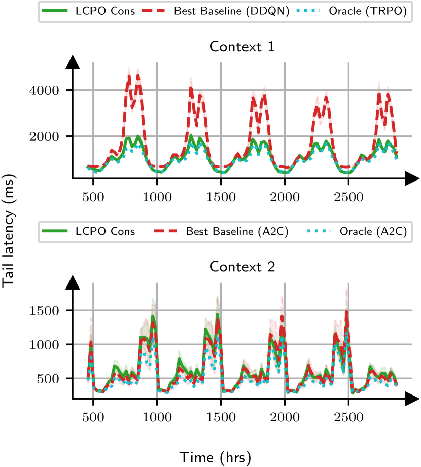
Figure 10: Tail latency with 95th percentile confidence intervals as training progresses (lower is better). We consider an initial learning period of 3.5 million samples. LCPO remains close to the oracle throughout contexts, while baselines suffer from non-stationarity.

B.2 Experiment Setup

We use the straggler mitigation environment from prior work (Hamadanian et al., 2022), with a similar configuration except with 9 actions (timeouts of $600^{ms}$ and $1000^{ms}$ added). Similar to §A.4, our implementations of A2C, TRPO, DDQN and SAC use the Pytorch (Paszke et al., 2019) library. Table 8 is a comprehensive list of all hyperparameters used in training and the environment.

All baselines were tuned on a separate workload. LCPO hyperparameters were copied from the gymnasium experiments, except for base entropy which was tuned with an informal search with a separate workload (not in the evaluation set).

Table 8: Training setup and hyperparameters for straggler mitigation experiments.

Group	Hyperparameter	Value
Neural network	Hidden layers	$\phi$ network: (32, 16)
		$\rho$ network: (32, 32)
	Hidden layer activation function	Relu
	Output layer activation function	Actors: Softmax, Critics and DDQN: Identity mapping
	Optimizer	Adam ($\beta_{1}=0.9$, $\beta_{2}=0.999$) (Kingma & Ba, 2017)
	Learning rate	0.001
	Weight decay	$10^{-4}$
RL training (general)	Random seeds	10
	$\lambda$ (for GAE in A2C and TRPO)	0.95
	$\gamma$	0.9
A2C	Rollout per epoch	4608
TRPO	Rollout per epoch	10240
	Damping coefficient	0.1
	Stepsize	0.01
DDQN	Rollout per epoch	128
	Batch Size	512
	Initial fully random period	1000 epochs
	$\epsilon$-greedy schedule	1 to 0 in 5000 epochs
	Polyak $\alpha$	0.01
	Buffer size $N$	All samples ($N=21M$)
SAC	Rollout per epoch	128
	Batch Size	512
	Initial fully random period	1000 epochs
	Base Entropy	0.01
	Entropy Target	$0.1\ln(9)$
	Log-Entropy Learning Rate	1e-3
	Polyak $\alpha$	0.005
	Buffer size $N$	All samples ($N=21M$)
LCPO	Rollout per epoch	128
	Base Entropy	0.01
	Entropy Target	$0.1\ln(9)$
	Log-Entropy Learning Rate	1e-3
	Buffer Size $n_{b}$	$210K$
	Damping coefficient	0.1
	$c_{anchor}$	0.0001
	$c_{recent}$	0.1
MBCD	h	300000 (default was 100/300)
	max_std	3 (default was 0.5)
	N (ensemble size)	5
	NN hidden layers	(64, 64, 64)
MBPO	M (model rollouts)	512
	N (ensemble size)	5
	k (rollout length)	1
	G (gradient steps)	1
Online EWC	averaging weight $\beta$	0.00007 (equivalent to $\sim 2M$ samples at rollout=128)
	scaling factor $\alpha$	0.1

References

- Alegre et al. (2021) Alegre, L. N., Bazzan, A. L., and da Silva, B. C. Minimum-delay adaptation in non-stationary reinforcement learning via online high-confidence change-point detection. In Proceedings of the 20th International Conference on Autonomous Agents and MultiAgent Systems, pp. 97–105, 2021.
- Atkinson et al. (2021) Atkinson, C., McCane, B., Szymanski, L., and Robins, A. Pseudo-rehearsal: Achieving deep reinforcement learning without catastrophic forgetting. Neurocomputing, 428:291–307, Mar 2021. ISSN 0925-2312. doi: 10.1016/j.neucom.2020.11.050. URL http://dx.doi.org/10.1016/j.neucom.2020.11.050.
- Caccia et al. (2020) Caccia, M., Rodriguez, P., Ostapenko, O., Normandin, F., Lin, M., Page-Caccia, L., Laradji, I. H., Rish, I., Lacoste, A., Vázquez, D., et al. Online fast adaptation and knowledge accumulation (osaka): a new approach to continual learning. Advances in Neural Information Processing Systems, 33:16532–16545, 2020.
- Caruana (1997) Caruana, R. Multitask learning. Machine learning, 28:41–75, 1997.
- Chaudhry et al. (2018) Chaudhry, A., Dokania, P. K., Ajanthan, T., and Torr, P. H. S. Riemannian Walk for Incremental Learning: Understanding Forgetting and Intransigence, pp. 556–572. Springer International Publishing, 2018. ISBN 9783030012526. doi: 10.1007/978-3-030-01252-6_33. URL http://dx.doi.org/10.1007/978-3-030-01252-6_33.
- Chen et al. (2022) Chen, X., Zhu, X., Zheng, Y., Zhang, P., Zhao, L., Cheng, W., Cheng, P., Xiong, Y., Qin, T., Chen, J., et al. An adaptive deep rl method for non-stationary environments with piecewise stable context. Advances in Neural Information Processing Systems, 35:35449–35461, 2022.
- da Silva et al. (2006) da Silva, B. C., Basso, E. W., Bazzan, A. L. C., and Engel, P. M. Dealing with non-stationary environments using context detection. In Proceedings of the 23rd International Conference on Machine Learning, ICML ’06, pp. 217–224, New York, NY, USA, 2006. Association for Computing Machinery. ISBN 1595933832. doi: 10.1145/1143844.1143872. URL https://doi.org/10.1145/1143844.1143872.
- Dietterich et al. (2018) Dietterich, T. G., Trimponias, G., and Chen, Z. Discovering and removing exogenous state variables and rewards for reinforcement learning. In International Conference on Machine Learning, 2018. URL https://api.semanticscholar.org/CorpusID:46938244.
- Doya et al. (2002) Doya, K., Samejima, K., Katagiri, K.-i., and Kawato, M. Multiple model-based reinforcement learning. Neural computation, 14(6):1347–1369, 2002.
- Duan et al. (2016) Duan, Y., Chen, X., Houthooft, R., Schulman, J., and Abbeel, P. Benchmarking deep reinforcement learning for continuous control. In International conference on machine learning, pp. 1329–1338. PMLR, 2016.
- Farajtabar et al. (2019) Farajtabar, M., Azizan, N., Mott, A., and Li, A. Orthogonal gradient descent for continual learning, 2019. URL https://arxiv.org/abs/1910.07104.
- Feng et al. (2022) Feng, F., Huang, B., Zhang, K., and Magliacane, S. Factored adaptation for non-stationary reinforcement learning. Advances in Neural Information Processing Systems, 35:31957–31971, 2022.
- Finn et al. (2019) Finn, C., Rajeswaran, A., Kakade, S., and Levine, S. Online meta-learning, 2019.
- Gu et al. (2016) Gu, S., Lillicrap, T., Ghahramani, Z., Turner, R. E., and Levine, S. Q-prop: Sample-efficient policy gradient with an off-policy critic. arXiv preprint arXiv:1611.02247, 2016.
- Gu et al. (2021) Gu, Z., She, C., Hardjawana, W., Lumb, S., McKechnie, D., Essery, T., and Vucetic, B. Knowledge-assisted deep reinforcement learning in 5g scheduler design: From theoretical framework to implementation. IEEE Journal on Selected Areas in Communications, 39(7):2014–2028, 2021.
- Haarnoja et al. (2018a) Haarnoja, T., Pong, V., Zhou, A., Dalal, M., Abbeel, P., and Levine, S. Composable deep reinforcement learning for robotic manipulation. In 2018 IEEE International Conference on Robotics and Automation (ICRA), pp. 6244–6251, 2018a. doi: 10.1109/ICRA.2018.8460756.
- Haarnoja et al. (2018b) Haarnoja, T., Zhou, A., Abbeel, P., and Levine, S. Soft actor-critic: Off-policy maximum entropy deep reinforcement learning with a stochastic actor. In International conference on machine learning, pp. 1861–1870. PMLR, 2018b.
- Haarnoja et al. (2018c) Haarnoja, T., Zhou, A., Hartikainen, K., Tucker, G., Ha, S., Tan, J., Kumar, V., Zhu, H., Gupta, A., Abbeel, P., and Levine, S. Soft actor-critic algorithms and applications, 2018c. URL https://arxiv.org/abs/1812.05905.
- Hamadanian et al. (2022) Hamadanian, P., Schwarzkopf, M., Sen, S., and Alizadeh, M. Reinforcement learning in time-varying systems: an empirical study, 2022. URL https://arxiv.org/abs/2201.05560.
- Hasselt et al. (2016) Hasselt, H. v., Guez, A., and Silver, D. Deep reinforcement learning with double q-learning. In Proceedings of the Thirtieth AAAI Conference on Artificial Intelligence, AAAI’16, pp. 2094–2100. AAAI Press, 2016.
- Haydari & Yılmaz (2022) Haydari, A. and Yılmaz, Y. Deep reinforcement learning for intelligent transportation systems: A survey. IEEE Transactions on Intelligent Transportation Systems, 23(1):11–32, 2022. doi: 10.1109/TITS.2020.3008612.
- He et al. (2020) He, X., Sygnowski, J., Galashov, A., Rusu, A. A., Teh, Y. W., and Pascanu, R. Task agnostic continual learning via meta learning. In 4th Lifelong Machine Learning Workshop at ICML 2020, 2020. URL https://openreview.net/forum?id=AeIzVxdJgeb.
- Heess et al. (2017) Heess, N., TB, D., Sriram, S., Lemmon, J., Merel, J., Wayne, G., Tassa, Y., Erez, T., Wang, Z., Eslami, S. M. A., Riedmiller, M., and Silver, D. Emergence of locomotion behaviours in rich environments, 2017. URL https://arxiv.org/abs/1707.02286.
- Isele & Cosgun (2018) Isele, D. and Cosgun, A. Selective experience replay for lifelong learning, 2018.
- Janner et al. (2021) Janner, M., Fu, J., Zhang, M., and Levine, S. When to trust your model: Model-based policy optimization, 2021.
- Kaplanis et al. (2018) Kaplanis, C., Shanahan, M., and Clopath, C. Continual reinforcement learning with complex synapses, 2018.
- Khetarpal et al. (2020) Khetarpal, K., Riemer, M., Rish, I., and Precup, D. Towards continual reinforcement learning: A review and perspectives. arXiv preprint arXiv:2012.13490, 2020.
- Kingma & Ba (2017) Kingma, D. P. and Ba, J. Adam: A method for stochastic optimization, 2017.
- Kirkpatrick et al. (2017) Kirkpatrick, J., Pascanu, R., Rabinowitz, N., Veness, J., Desjardins, G., Rusu, A. A., Milan, K., Quan, J., Ramalho, T., Grabska-Barwinska, A., et al. Overcoming catastrophic forgetting in neural networks. Proceedings of the national academy of sciences, 114(13):3521–3526, 2017.
- Lee et al. (2018) Lee, K., Lee, K., Lee, H., and Shin, J. A simple unified framework for detecting out-of-distribution samples and adversarial attacks, 2018. URL https://arxiv.org/abs/1807.03888.
- Mahalanobis (2018) Mahalanobis, P. C. On the generalized distance in statistics. Sankhyā: The Indian Journal of Statistics, Series A (2008-), 80:S1–S7, 2018.
- Mao et al. (2017) Mao, H., Netravali, R., and Alizadeh, M. Neural adaptive video streaming with pensieve. In Proceedings of the Conference of the ACM Special Interest Group on Data Communication, pp. 197–210, 2017.
- Mao et al. (2018a) Mao, H., Schwarzkopf, M., Venkatakrishnan, S. B., Meng, Z., and Alizadeh, M. Learning scheduling algorithms for data processing clusters, 2018a. URL https://arxiv.org/abs/1810.01963.
- Mao et al. (2018b) Mao, H., Venkatakrishnan, S. B., Schwarzkopf, M., and Alizadeh, M. Variance reduction for reinforcement learning in input-driven environments, 2018b. URL https://arxiv.org/abs/1807.02264.
- Mao et al. (2019) Mao, H., Schwarzkopf, M., Venkatakrishnan, S. B., Meng, Z., and Alizadeh, M. Learning scheduling algorithms for data processing clusters. In Proceedings of the ACM Special Interest Group on Data Communication, SIGCOMM ’19, pp. 270–288, New York, NY, USA, 2019. Association for Computing Machinery. ISBN 9781450359566. doi: 10.1145/3341302.3342080. URL https://doi.org/10.1145/3341302.3342080.
- Marcus et al. (2019) Marcus, R., Negi, P., Mao, H., Zhang, C., Alizadeh, M., Kraska, T., Papaemmanouil, O., and Tatbul, N. Neo: A learned query optimizer. arXiv preprint arXiv:1904.03711, 2019.
- McCloskey & Cohen (1989) McCloskey, M. and Cohen, N. J. Catastrophic interference in connectionist networks: The sequential learning problem. Psychology of Learning and Motivation, 24:109–165, 1989. ISSN 0079-7421. doi: https://doi.org/10.1016/S0079-7421(08)60536-8. URL https://www.sciencedirect.com/science/article/pii/S0079742108605368.
- Mnih et al. (2013) Mnih, V., Kavukcuoglu, K., Silver, D., Graves, A., Antonoglou, I., Wierstra, D., and Riedmiller, M. Playing atari with deep reinforcement learning. arXiv preprint arXiv:1312.5602, 2013.
- Mnih et al. (2016) Mnih, V., Badia, A. P., Mirza, M., Graves, A., Lillicrap, T., Harley, T., Silver, D., and Kavukcuoglu, K. Asynchronous methods for deep reinforcement learning. In International conference on machine learning, pp. 1928–1937. PMLR, 2016.
- Nagabandi et al. (2019) Nagabandi, A., Finn, C., and Levine, S. Deep online learning via meta-learning: Continual adaptation for model-based rl, 2019.
- Padakandla et al. (2020) Padakandla, S., J., P. K., and Bhatnagar, S. Reinforcement learning algorithm for non-stationary environments. Applied Intelligence, 50(11):3590–3606, jun 2020. doi: 10.1007/s10489-020-01758-5. URL https://doi.org/10.1007%2Fs10489-020-01758-5.
- Pan et al. (2022) Pan, M., Zhu, X., Wang, Y., and Yang, X. Iso-dream: Isolating noncontrollable visual dynamics in world models. In Oh, A. H., Agarwal, A., Belgrave, D., and Cho, K. (eds.), Advances in Neural Information Processing Systems, 2022. URL https://openreview.net/forum?id=6LBfSduVg0N.
- Parisi et al. (2019) Parisi, G. I., Kemker, R., Part, J. L., Kanan, C., and Wermter, S. Continual lifelong learning with neural networks: A review. Neural Networks, 113:54–71, 2019. ISSN 0893-6080. doi: https://doi.org/10.1016/j.neunet.2019.01.012. URL https://www.sciencedirect.com/science/article/pii/S0893608019300231.
- Paszke et al. (2019) Paszke, A., Gross, S., Massa, F., Lerer, A., Bradbury, J., Chanan, G., Killeen, T., Lin, Z., Gimelshein, N., Antiga, L., Desmaison, A., Kopf, A., Yang, E., DeVito, Z., Raison, M., Tejani, A., Chilamkurthy, S., Steiner, B., Fang, L., Bai, J., and Chintala, S. Pytorch: An imperative style, high-performance deep learning library. In Wallach, H., Larochelle, H., Beygelzimer, A., d'Alché-Buc, F., Fox, E., and Garnett, R. (eds.), Advances in Neural Information Processing Systems 32, pp. 8024–8035. Curran Associates, Inc., 2019. URL http://papers.neurips.cc/paper/9015-pytorch-an-imperative-style-high-performance-deep-learning-library.pdf.
- Pathak et al. (2017) Pathak, D., Agrawal, P., Efros, A. A., and Darrell, T. Curiosity-driven exploration by self-supervised prediction, 2017. URL https://arxiv.org/abs/1705.05363.
- Pinto et al. (2017) Pinto, L., Davidson, J., Sukthankar, R., and Gupta, A. Robust adversarial reinforcement learning, 2017. URL https://arxiv.org/abs/1703.02702.
- Podolskiy et al. (2021) Podolskiy, A., Lipin, D., Bout, A., Artemova, E., and Piontkovskaya, I. Revisiting mahalanobis distance for transformer-based out-of-domain detection, 2021. URL https://arxiv.org/abs/2101.03778.
- Poiani et al. (2021) Poiani, R., Tirinzoni, A., Restelli, M., et al. Meta-reinforcement learning by tracking task non-stationarity. In IJCAI, pp. 2899–2905. International Joint Conferences on Artificial Intelligence, 2021.
- Raffin (2020) Raffin, A. Rl baselines3 zoo. https://github.com/DLR-RM/rl-baselines3-zoo, 2020.
- Raffin et al. (2021) Raffin, A., Hill, A., Gleave, A., Kanervisto, A., Ernestus, M., and Dormann, N. Stable-baselines3: Reliable reinforcement learning implementations. Journal of Machine Learning Research, 22(268):1–8, 2021. URL http://jmlr.org/papers/v22/20-1364.html.
- Ren et al. (2022) Ren, H., Sootla, A., Jafferjee, T., Shen, J., Wang, J., and Bou Ammar, H. Reinforcement learning in presence of discrete markovian context evolution, 02 2022.
- Rolnick et al. (2019) Rolnick, D., Ahuja, A., Schwarz, J., Lillicrap, T. P., and Wayne, G. Experience replay for continual learning, 2019.
- Rusu et al. (2016) Rusu, A. A., Rabinowitz, N. C., Desjardins, G., Soyer, H., Kirkpatrick, J., Kavukcuoglu, K., Pascanu, R., and Hadsell, R. Progressive neural networks. arXiv preprint arXiv:1606.04671, 2016.
- Schulman et al. (2015) Schulman, J., Levine, S., Moritz, P., Jordan, M. I., and Abbeel, P. Trust region policy optimization, 2015. URL https://arxiv.org/abs/1502.05477.
- Schulman et al. (2018) Schulman, J., Moritz, P., Levine, S., Jordan, M., and Abbeel, P. High-dimensional continuous control using generalized advantage estimation, 2018.
- Schwarz et al. (2018) Schwarz, J., Luketina, J., Czarnecki, W. M., Grabska-Barwinska, A., Teh, Y. W., Pascanu, R., and Hadsell, R. Progress & compress: A scalable framework for continual learning, 2018.
- Sinclair et al. (2023) Sinclair, S. R., Frujeri, F., Cheng, C.-A., Marshall, L., Barbalho, H., Li, J., Neville, J., Menache, I., and Swaminathan, A. Hindsight learning for mdps with exogenous inputs. In Proceedings of the 40th International Conference on Machine Learning, ICML’23. JMLR.org, 2023.
- Sutton & Barto (2018) Sutton, R. S. and Barto, A. G. Reinforcement Learning: An Introduction. A Bradford Book, Cambridge, MA, USA, 2018. ISBN 0262039249.
- Tang & Agrawal (2019) Tang, Y. and Agrawal, S. Discretizing continuous action space for on-policy optimization, 2019. URL https://arxiv.org/abs/1901.10500.
- Towers et al. (2023) Towers, M., Terry, J. K., Kwiatkowski, A., Balis, J. U., Cola, G. d., Deleu, T., Goulão, M., Kallinteris, A., KG, A., Krimmel, M., Perez-Vicente, R., Pierré, A., Schulhoff, S., Tai, J. J., Shen, A. T. J., and Younis, O. G. Gymnasium, March 2023. URL https://zenodo.org/record/8127025.
- Uhlenbeck & Ornstein (1930) Uhlenbeck, G. E. and Ornstein, L. S. On the theory of the brownian motion. Phys. Rev., 36:823–841, Sep 1930. doi: 10.1103/PhysRev.36.823. URL https://link.aps.org/doi/10.1103/PhysRev.36.823.
- Vitter (1985) Vitter, J. S. Random sampling with a reservoir. ACM Transactions on Mathematical Software (TOMS), 11(1):37–57, 1985.
- Zeng et al. (2019) Zeng, G., Chen, Y., Cui, B., and Yu, S. Continual learning of context-dependent processing in neural networks. Nature Machine Intelligence, 1(8):364–372, 2019.
- Zhang et al. (2021) Zhang, H., Zhou, A., Hu, Y., Li, C., Wang, G., Zhang, X., Ma, H., Wu, L., Chen, A., and Wu, C. Loki: Improving long tail performance of learning-based real-time video adaptation by fusing rule-based models. In Proceedings of the 27th Annual International Conference on Mobile Computing and Networking, MobiCom ’21, pp. 775–788, New York, NY, USA, 2021. Association for Computing Machinery. ISBN 9781450383424. doi: 10.1145/3447993.3483259. URL https://doi.org/10.1145/3447993.3483259.
- Zhang et al. (2023) Zhang, J., Zheng, Y., Zhang, C., Zhao, L., Song, L., Zhou, Y., and Bian, J. Robust situational reinforcement learning in face of context disturbances. In Proceedings of the 40th International Conference on Machine Learning (ICML), September 2023. URL https://www.microsoft.com/en-us/research/publication/robust-situational-reinforcement-learning-in-face-of-context-disturbances/.
- Zhu et al. (2020) Zhu, H., Yu, J., Gupta, A., Shah, D., Hartikainen, K., Singh, A., Kumar, V., and Levine, S. The ingredients of real-world robotic reinforcement learning, 2020. URL https://arxiv.org/abs/2004.12570.
- Zintgraf et al. (2019) Zintgraf, L., Shiarli, K., Kurin, V., Hofmann, K., and Whiteson, S. Fast context adaptation via meta-learning. In International Conference on Machine Learning, pp. 7693–7702. PMLR, 2019.