Model Stitching and Visualization
How GAN Generators can Invert Networks in Real-Time

Abstract

Critical applications, such as in the medical field, require the rapid provision of additional information to interpret decisions made by deep learning methods. In this work, we propose a fast and accurate method to visualize activations of classification and semantic segmentation networks by stitching them with a GAN generator utilizing convolutions. We test our approach on images of animals from the AFHQ wild dataset and real-world digital pathology scans of stained tissue samples. Our method provides comparable results to established gradient descent methods on these datasets while running about two orders of magnitude faster.

1 Introduction

Interpretability of neural networks and understanding what features they extract from the input are crucial, especially in critical applications like healthcare. Additionally, the availability of this information in near real-time is often required. In this work, we efficiently visualize the extracted features of a ResNet50 (He et al., 2016) classification network trained on ImageNet (Deng et al., 2009) and a ResNet34 (He et al., 2016) backbone semantic segmentation network trained on digital pathology scans of histochemically stained tissue samples, by inverting them using a generative adversarial network (GAN) (Goodfellow et al., 2014). A StyleGAN2 architecture (Karras et al., 2020) is used in this role.

We observe that the features learned by the classification or semantic segmentation network are compatible with the features learned by a GAN generator trained in an unsupervised manner, even though the classification or semantic segmentation network and the GAN were trained completely unaware of each other. In order to bring the two models together, we learn a linear transformation, to be more precise, a 1x1 convolution, to stitch them. The 1x1 convolution is trained to map from a hidden layer of the classification or semantic segmentation network into a hidden layer of the GAN generator. Utilizing this mapping, we can quickly visualize activations of the classification or semantic segmentation network, by transferring them through the convolutional connection into the GAN generator, i.e., we use the GAN generator as a decoder to invert the classification or semantic segmentation network.

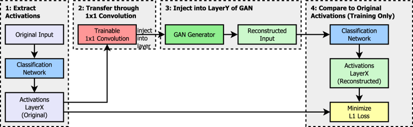
Figure 1: Usage and training process for stitching a GAN generator and a classification network in a hidden layer.

2 Related Work

We use model stitching (Lenc & Vedaldi, 2015) to stitch a classification or semantic segmentation network with a GAN in order to visualize activations of the classification or semantic segmentation network in real-time. A 1x1 convolution is used as the stitching layer, which is methodically closely related to (Bansal et al., 2021). The work of (Bansal et al., 2021) applied a sequence of batch norm, 1x1 convolution, and batch norm to stitch two image classification networks together in a hidden layer. We do the stitching in order to see how similar the learned representations of hidden layers of a classification network or semantic segmentation network are to the learned representations of hidden layers of a GAN generator. In addition, we visualize activations of the classification or semantic segmentation network by sending them through the GAN generator.

Activations can also be visualized through gradient descent (Mahendran & Vedaldi, 2014). The disadvantage is that it is slow since it needs several forward-backward passes through the network. We use gradient descent as in (Olah et al., 2017) and gradient descent without any regularization as baselines, to compare our GAN method against. Another method is to visualize the activations by training a decoder network to invert the classification network from a hidden layer (Dosovitskiy & T.Brox, 2016). But such approach makes it necessary to train a new decoder for every new layer in the classification network that should be visualized. In contrast, with our method, it is only necessary to train a new 1x1 convolution and keep the same GAN generator. Finally, in the work of (Dosovitskiy & T.Brox, 2016), the decoder was trained to minimize a reconstruction error in the input space of the classification network, whereas we train the stitching layer to minimize a reconstruction error at the hidden layer where we transfer from.

3 Methodology

In this section, we show an overview of our method and the gradient descent we use as a baseline and describe the evaluation metrics we use in the experiments.

3.1 Overview

Figure 1 shows an overview of our approach. For combining a classification network with a GAN generator in a hidden layer, i.e., stitching LayerX of the classifier and LayerY of the GAN generator, we train a 1x1 convolution to transfer between the two layers. After the 1x1 convolution is trained, we can invert the classification network at LayerX by forward transferring the activations through LayerY of the GAN generator, as shown in steps 1 - 3 in Figure 1.

First, the activations at LayerX are extracted. Then we transfer them through the 1x1 convolution to get them from the latent space of LayerX into the latent space of LayerY. After that, the activations are scaled to match the spatial size of LayerY. For example, layer b32.conv0 of StyleGAN2 has a spatial size of 32x32. Therefore, before injecting our activations into that layer, we scale them to a spatial size of 32x32 via nearest neighbor scaling. Finally, we inject the activations into LayerY of the GAN generator while generating an output with the generator from a random seed. This means that we still get variations from the used seed after the injection layer. The output of the GAN generator is an inversion referred to as reconstructed input in Figure 1.

For training, we need to compare the reconstructed and original input and train the 1x1 convolution to minimize a loss between the two. To compare them, we again use the classification network, as shown in step 4 in Figure 1, and optimize the 1x1 convolution to minimize the L1 loss in LayerX. We do not minimize a loss in the input layer since we expect that, as the input propagates deeper through the network, it should discard unnecessary low-level information (e.g., the individual position of the dots on leopard fur), which the network would then be unable to reconstruct properly. Since we aim to visualize the activations of LayerX, we also use this layer to compute the loss.

3.2 Evaluation

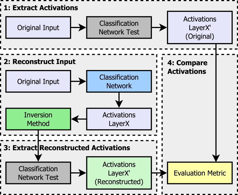
Figure 2: Comparing inversion methods.

To evaluate how good our GAN-based inversion method is, we compare it to gradient descent with regularization (in the following referred to as FFT DEC) and gradient descent without regularization (in the following referred to as PLAIN). Similar to the training, we do not compare the original input and the result of the inversion method in the input layer but in a hidden layer of a second classification network. The motivation here is that we want to know how accurately the features extracted by LayerX have been reconstructed rather than whether it also matches low-level features LayerX has already discarded. In addition, the comparison is made in LayerX’ of a second network, since we want to avoid the effects of adversarial examples.

The whole process is shown in Figure 2. First, we extract the activations $\alpha^{x}$ from the original input from the test network at LayerX’. Second, we reconstruct the activations at LayerX from the network we wish to interpret. Third, we pass the reconstruction in the test network and extract its activation $\alpha^{x}{}^{\prime}$ at LayerX’. Lastly, we compare both activations from the test network.

3.3 Gradient Descent

Algorithm 1 Inverting from LayerX

  Input: data $x$, network till LayerX $F_{X}$, L1 loss $L$

  $y\leftarrow F_{X}(x)$

  $z^{\prime}_{0}\leftarrow noise$

  optimizer watches $z^{\prime}_{0}$

  for $i\leftarrow 0$ to $n$ do

     $\text{loss}\leftarrow\nabla_{z^{\prime}_{i}}[L(F_{X}(g(\sigma(h(z^{\prime}_{i})))),y)]$ (*)

     backpropagate loss

     optimizer does update step on $z^{\prime}_{i}$

  end for

Algorithm 1 describes how we perform gradient descent with the FFT DEC and PLAIN methods. For the PLAIN method, both the functions $g$ and $h$ in (*) are the identity, and $\sigma$ is the sigmoid function (to keep the values of the inversion in the 0 to 1 range). For the FFT DEC method, $h$ is an inverse Fourier transform followed by correlating colors (so that $z^{\prime}$ is in color de-correlated Fourier space), and $g$ is one-pixel jittering to reduce noise in the inversion. With one-pixel jittering, we first pad the input by 2 pixels on each side and then randomly move it up to one pixel horizontally and vertically. We perform $n=512$ forward-backward passes through the classification or semantic segmentation network and use the Adam optimizer (Kingma & Ba, 2015) with a learning rate of 0.05.

3.4 Evaluation Metrics

Let $x\in I$ be the original input image, $F_{X}$ the classification or semantic segmentation network till LayerX (the layer from which we want to reconstruct the activations), $L_{X}$ the latent space of LayerX, $g:L_{X}\rightarrow I$ an inversion method (steps 2 - 3 in Figure 1 or gradient descent), and $F_{X}^{\prime}$ the test network till LayerX’.

We compare activations $\alpha^{x}{}^{\prime}=F_{X}^{\prime}(g(F_{X}(x)))$ and $\alpha^{x}=F_{X}^{\prime}(x)$ by computing a similarity metric $d(\alpha^{x}{}^{\prime},\alpha^{x})$ with $d:L_{X}^{\prime}\times L_{X}^{\prime}\rightarrow\mathbb{R}$. For $d$, we use the following three evaluation metrics:

• Cosine similarity: Let $C$ be a matrix of shape (H, W) with

  $$C_{ij}=\frac{\alpha^{x}{}^{\prime}[:,i,j]\cdot\alpha^{x}{}[:,i,j]}{\text{max}(||\alpha^{x}{}^{\prime}[:,i,j])||_{2}\cdot||\alpha^{x}{}[:,i,j])||_{2},\epsilon}.$$

  Then $d(\alpha^{x}{}^{\prime},\alpha^{x})=\text{mean}(C)$. This means we first compute pixelwise cosine similarity, followed by the computation of the mean of the resulting matrix.

• L1 loss: $d(\alpha_{x}^{\prime},\alpha_{x})=\text{mean}(|\alpha_{x}^{\prime}-\alpha_{x}|$)

• Cosine similarity gram matrices: We first compute the gram matrices for $\alpha_{x}^{\prime}$ and $\alpha_{x}$. Let $G(\alpha)$ be the gram matrix for $\alpha$, then $G(\alpha)_{ij}=\text{dot}(\text{vec}(\alpha[i]),\text{vec}(\alpha[j]))$ with $\alpha[i]$ being the i-th channel of $\alpha$ and the vec function flattening it into a vector ($\alpha[i]$ is a matrix of shape (H, W) and vec flattens it to a vector of shape $(H\cdot W)$. Then:
  

  $$d(\alpha_{x}^{\prime},\alpha_{x})=\text{sum}\left(\frac{G(\alpha_{x}^{\prime})\cdot G(\alpha_{x})}{\text{max}(||G(\alpha_{x}^{\prime})||_{2}\cdot||G(\alpha_{x})||_{2},\epsilon)}\right)$$

Both cosine similarity and L1 loss work pixelwise. They measure whether concepts have been correctly reconstructed and also whether they have been reconstructed at the correct position. The similarity between gram matrices can be used for style transfer (Gatys et al., 2015). Therefore, with cosine similarity between gram matrices, we measure how well the concepts present in the original image have been reconstructed without depending on whether they have been correctly reconstructed spatially.

4 Experiments

Figure 3: Reconstructing the input from activations at the output of Layer3 of ResNet50. Top row shows the original dataset images, middle line shows their reconstructions with the GAN method, bottom line shows their reconstructions with FFT DEC.

Table 1: Results for the AFHQ wild data.

layer	Method	AFHQ
		Cosine Similarity	Cosine Similarity Gram Matrices	L1 Loss	Evaluation Time
Layer1	gan	0.954$\pm$ 0.008	0.996$\pm$ 0.002	0.162 $\pm$ 0.019	7s
	fft dec	0.932$\pm$ 0.010	0.985$\pm$ 0.002	0.199 $\pm$ 0.023	509s
	plain	0.973$\pm$ 0.006	0.989$\pm$ 0.004	0.120 $\pm$ 0.016	497s
Layer2	gan	0.878$\pm$ 0.015	0.987$\pm$ 0.005	0.135 $\pm$ 0.011	7s
	fft dec	0.903$\pm$ 0.009	0.981$\pm$ 0.004	0.121 $\pm$ 0.008	606s
	plain	0.928$\pm$ 0.010	0.976$\pm$ 0.006	0.101 $\pm$ 0.009	598s
Layer3	gan	0.778$\pm$ 0.032	0.928$\pm$ 0.016	0.070 $\pm$ 0.007	7s
	fft dec	0.831$\pm$ 0.024	0.925$\pm$ 0.018	0.060 $\pm$ 0.006	713s
	plain	0.729$\pm$ 0.040	0.823$\pm$ 0.033	0.080 $\pm$ 0.008	701s
Layer4	gan	0.527$\pm$ 0.117	0.518$\pm$ 0.179	0.868 $\pm$ 0.108	7s
	fft dec	0.665$\pm$ 0.053	0.645$\pm$ 0.078	0.808 $\pm$ 0.082	743s
	plain	0.319$\pm$ 0.024	0.170$\pm$ 0.023	0.987 $\pm$ 0.059	746s

4.1 Setup

In this section, we describe the datasets, models, and hardware we use in our experiments.

4.1.1 Datasets

Table 2: Train- and Validationset sizes for the two datasets (Digipath and AFHQ wild) we use in this work.

	Digipath	AFHQ wild
Training Size	$156\,680$	$4738$
Validation Size	$300$	$500$

We conduct our experiments on two different datasets, once on tissue scans in digital pathology data (Digipath) and once on Animal Faces-HQ (AFHQ) containing wild animal faces (Choi et al., 2020). The images in the Digipath data have a spatial size of 600x600, whereas the AFHQ wild images have a size of 512x512 (and we downsample them from 512x512 to 224x224). We use an in-house dataset and models that are not openly available for our experiments on digital pathology data. For the AFHQ data, we use the original Animal Faces dataset available on Kaggle. Table 2 shows the number of training and validation samples for both datasets we used.

4.1.2 Hardware and Software

For all our experiments, we use a Linux server with 4 Nvidia RTX A6000 GPUs. On the software side, we use PyTorch (Paszke et al., 2019) version 1.11.0 and Torchvision version 0.12.0.

4.1.3 Training

All networks in our experiments are in eval mode, and in training, we only train a 1x1 convolution to map between two layers. We use Adam with a learning rate of 0.01 as an optimizer, and train with a batch size of 8.

4.2 AFHQ Dataset Results

Figure 4: Reconstructing activations from Layer1 to Layer4 with our GAN-based method.

In this section, we describe our results from the experiments on the AFHQ wild data. We stitch a ResNet50 from Torchvision models, trained on ImageNet, with a StyleGAN2 trained on AFHQ wild data, and compare the results to gradient descent with and without regularization. As the test network, we use a ResNet34 from Torchvision models trained on ImageNet. The stitching is performed at 4 points of the ResNet50, namely at the output of Layer1 to Layer4, and each time we train for 30 epochs. In Table 1, we report the metrics on the validation data for the epoch which had the highest cosine similarity on the validation data.

Table 1 shows the result of different metrics when inverting a ResNet50 classifier trained on ImageNet data. It compares different inversion methods and measures their run time for the 500 validation images of the AFHQ data. We do the reconstruction at the output of Layer1 to Layer4 of ResNet50 (shown in the ”layer” column), each time with three different methods: forward transferring through StyleGAN2 (GAN), by gradient descent in color de-correlated Fourier space and randomly moving the image one pixel in every update step (FFT DEC), and by gradient descent without any regularization (PLAIN). For the GAN method, we need not only a starting layer in ResNet50 but also a layer we want to stitch into in StyleGAN2. For the layer we stitch into, we choose the first convolution of a layer that is the same number of samplings away from the output as the layer in ResNet50 is away from the input. That means we stitch

• ResNet50 Layer1 $\rightarrow$ StyleGAN2 b128.conv0 (Layer1 is two downsampling steps from the input of ResNet50 away, and b128.conv0 is two upsampling steps from the output of StyleGAN2 away)

• ResNet50 Layer2 $\rightarrow$ StyleGAN2 b64.conv0

• ResNet50 Layer3 $\rightarrow$ StyleGAN2 b32.conv0

• ResNet50 Layer4 $\rightarrow$ StyleGAN2 b16.conv0

Each metric (cosine similarity, cosine similarity gram matrices, L1 loss) is evaluated for each of the $500$ images, and the table shows the mean $\pm$ standard deviation.

The GAN method takes considerably less time than the gradient descent methods (as shown in the ”Evaluation Time” column). For measuring the time for the GAN method, we let it run over the dataset 20 times and take the mean run time. The reported evaluation time also includes the time for computing the three evaluation metrics. For example, for Layer3, the GAN method takes 7 seconds, whereas gradient descent takes more than 700 seconds. In our experiments, we observed an average runtime improvement of 89x with a minimum improvement of 68x and a maximum improvement of 105x compared to PLAIN gradient descent. Similar improvements can also be observed compared to FFT DEC gradient descent. In this case, we observed an average runtime improvement of 90x with a minimum of 70x and a maximum of 104x. Our method runs faster because it only needs one forward pass through the classification network and the GAN generator, instead of 512 forward-backward passes through the classification network with gradient descent.

Table 3: Results for Digipath data.

layer	Method	Digipath
		Cosine Similarity	Cosine Similarity Gram Matrices	L1 Loss	Evaluation Time
Layer1	gan	0.896 $\pm$ 0.018	0.985 $\pm$ 0.009	0.601 $\pm$ 0.100	14s
	fft dec	0.825 $\pm$ 0.043	0.997 $\pm$ 0.001	0.786 $\pm$ 0.189	1112s
	plain	0.721 $\pm$ 0.098	0.946 $\pm$ 0.074	0.948 $\pm$ 0.067	1044s
Layer2	gan	0.857 $\pm$ 0.028	0.982$\pm$ 0.007	0.731 $\pm$ 0.089	10s
	fft dec	0.832 $\pm$ 0.037	0.982 $\pm$ 0.017	0.771 $\pm$ 0.057	1306s
	plain	0.691 $\pm$ 0.045	0.908 $\pm$ 0.030	1.069 $\pm$ 0.053	1237s
Layer3	gan	0.808 $\pm$ 0.035	0.959 $\pm$ 0.015	0.904 $\pm$ 0.084	11s
	fft dec	0.795 $\pm$ 0.023	0.909 $\pm$ 0.033	0.931 $\pm$ 0.069	1496s
	plain	0.489 $\pm$ 0.047	0.550 $\pm$ 0.088	1.482 $\pm$ 0.156	1426s
Layer4	gan	0.743 $\pm$ 0.067	0.859 $\pm$ 0.068	0.788 $\pm$ 0.086	10s
	fft dec	0.711 $\pm$ 0.055	0.793 $\pm$ 0.068	0.842 $\pm$ 0.074	1584s
	plain	0.317 $\pm$ 0.060	0.238 $\pm$ 0.075	1.403 $\pm$ 0.141	1513s

Usually, the GAN method performs best for the cosine similarity between gram matrices of activations metric (except for Layer4). In deeper layers (Layer3 and Layer4), FFT DEC performs best in cosine similarity and L1 loss. In earlier layers, it is worse than gradient descent without any regularization, due to the effect of one-pixel jittering (without it in Layer2 we get an L1 loss for FFT DEC of 0.078 vs. 0.101 for PLAIN and in Layer1 0.096 vs. 0.120 for PLAIN, both times outperforming PLAIN). We use the one-pixel jittering to reduce noise in the reconstruction, but it forces that even if we move the reconstruction one pixel, it should still have similar activations in the hidden layer and combining that with the fact that 1x1 (and to some extent also 3x3) convolutions with stride 2 utilize pixels in a grid pattern, likely reduces the evaluation score for the AFHQ wild data.

Figure 3 shows 8 samples for reconstructing activation from Layer3 with the GAN method and FFT DEC (we show the 8 samples where the GAN method has the highest cosine similarity out of the 500 validation samples). We can see that the GAN method does not introduce noise in the image, whereas FFT DEC does. But the GAN method loses lighting and some color information.

Figure 4 shows reconstructions with our GAN method for Layer1 to Layer4. The top line shows the original images, and the following four lines show reconstructions from Layer1 to Layer4. Each column for the AFHQ wild data uses the same noise seed (same $z$ vector for StyleGAN2), and the same noise seed is also used in Figure 8. The reconstruction works, except for Layer4 for the AFHQ wild data, where it is reduced to a fur pattern (tiger fur pattern for a tiger image and leopard fur pattern for a leopard image). For Layer1 and Layer2, it mainly retains lower level information like the fur pattern of a leopard (the image becomes slightly blurred by reconstructing it from Layer2). In contrast, in Layer3, it hallucinates a new fur pattern, and the image becomes sharper again. It is also interesting that for Layer4, the reconstructions for the AFHQ wild data are broken, whereas, for the Digipath data, they still resemble the general shape of the original input image. That may be because the StyleGAN2 was only trained on AFHQ wild data. In contrast, the ResNet50 we want to interpret was trained on ImageNet (much more variety of concepts), whereas, for the Digipath data, both the GAN and the segmentation network were trained on primarily the same data.

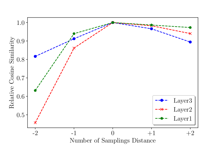
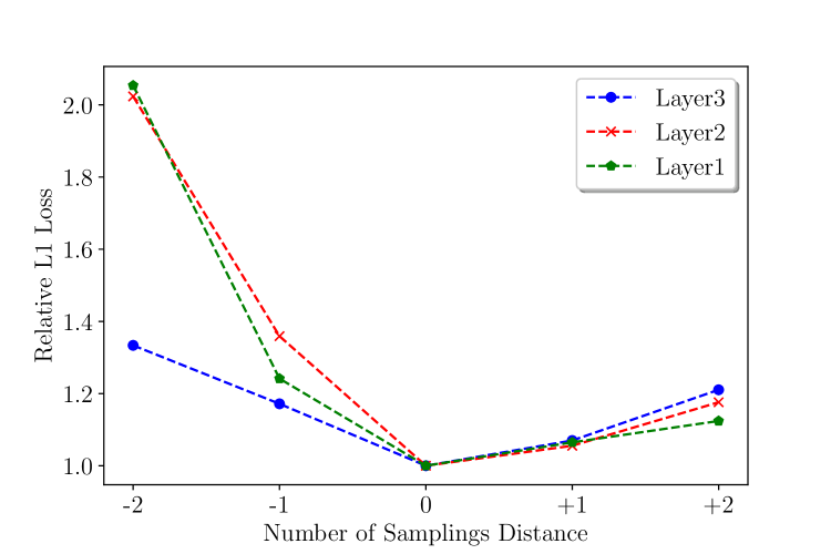
Figure 5: Result for stitching into different target layers. Top line shows results for AFHQ wild data, bottom line for Digipath data.

4.3 Digipath Dataset Results

In this section, we describe our results for the digital pathology data.

4.3.1 Models

We stitch a semantic segmentation network using a ResNet34 backbone trained to segment different diseases in tissue slides in digital pathology, with a GAN generator trained unsupervised to generate tissue slides. For the test network, we use a slightly modified ResNet34 as the backbone and replaced the 3x3 convolutional downsamplings with bilinear downsampling followed by a 3x3 stride 1 convolution. Further, we removed the 1x1 convolutional downsampling skip connections and the max pooling layer. Those adjustments were made to reduce noise in the gradient.

4.3.2 Results

We train the 1x1 convolution for $240\,000$ samples (for the AFHQ data, we trained for $142\,140$ samples). Table 3 shows our results evaluated on 300 images of the Digipath data. The table can be read similarly to Table 1. Again, the GAN method takes considerably less time than the gradient descent methods. We observed an average speedup of 120x with a minimum improvement of 76x and a maximum of 147x compared to PLAIN. Moreover, we observed a similar speedup compared to FFT DEC, with an average improvement of 126x, a minimum of 81x, and a maximum of 154x.

Two results are noticeably different compared to the results for the AFHQ data. First, the GAN method performs best in the cosine similarity and L1 loss metrics over all layers, whereas for the AFHQ data, it does not perform best even for any layer. Second, gradient descent without regularization (PLAIN) performs considerably worse here compared to FFT DEC, even in the earlier layers. A likely reason for those two differences is that the test network we use for the Digipath data does not use convolutional downsampling but bilinear downsampling. Removing the max pooling layer and the 1x1 convolutional downsamplings in the skip connection and replacing the 3x3 convolutional downsamplings with bilinear downsamplings followed by a 3x3 stride 1 convolution dramatically reduces noise in inversions with gradient descent, as shown in Figure 6.

1x1 stride 2 convolutions only utilize one-quarter of the input pixels in a grid pattern. Three-quarters of the input pixels remain unused. Those three-quarters will receive zero gradients, leading to a checkerboard noise pattern in the gradient. 3x3 stride 2 convolutions can also utilize some pixels more than others, based on a grid pattern (Odena et al., 2016). For the AFHQ data, both ResNet50 and ResNet34 use convolutional downsamplings and share the same grid pattern. However, for the Digipath data, the test network does not use convolutional downsamplings, which means it is not assigning a magnitude of importance to pixels based on grid patterns, like the network we invert is doing. For this reason, we think that the noise patterns that gradient descent without any regularization (and to some extent also FFT DEC) is building into the inverted image do not transfer very well over to the test network. As a result, the gradient descent inversions perform worse compared to the GAN method. Consequently, since gradient descent without any regularization (PLAIN) is building in more noise, it is even stronger penalized in the metrics and performs considerably worse compared to the AFHQ data.

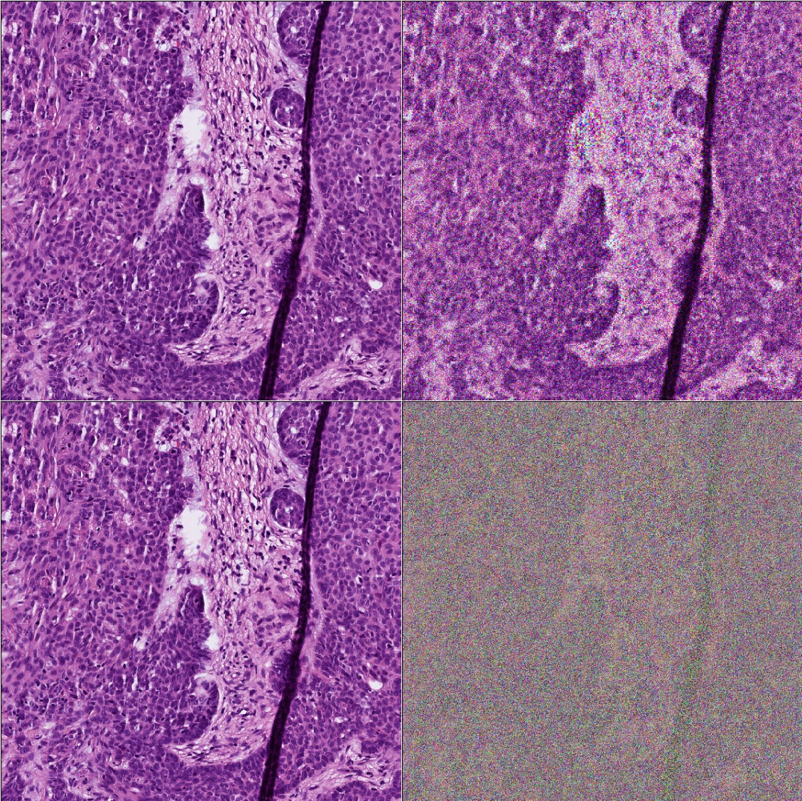
Figure 6: Comparison between inverting ResNet34 and bilinearResNet34 from Layer2. Top line shows the result for bilinearResNet34, bottom line for ResNet34. Left is both times the real input image, on the right is the resulting inversion. Both networks are randomly initialized and they are untrained.

4.4 Different End Layer

So far, we have stitched only into one GAN layer for a given classification or segmentation network layer. Here we evaluate the results of stitching from one layer of the classification or segmentation network into different layers of the GAN. Figure 5 shows the relative cosine similarity and L1 loss of reconstructions when stitching into different layers of StyleGAN2 (top line), and the GAN generator we use for the Digipath data (bottom line). In Table 1 and Table 3, we stitch into a layer of the GAN generator which has the same number of samplings distance from the output, as the layer in the classification or segmentation network we start from has from the input. That combination would correspond to a ”Number of Sampling Distance” of 0 in Figure 5. Here, -1 means we stitch into a layer in the GAN generator, which is one upsampling step further away from the output of the generator, and +1 means we stitch into a layer which is one upsampling step closer to the output of the generator. As an example, Table 4 shows the different target layers in StyleGAN2 when starting from Layer3 of ResNet50.

Table 4: Target layers in StyleGAN2 when starting from Layer3.

Number of Samplings Distance	Target layer
+2	b128.conv0
+1	b64.conv0
0	b32.conv0
-1	b16.conv0
-2	b8.conv0

We plot the values relative to the value at 0 distance and before plotting, we divide the value by the value at 0 distance. For the AFHQ wild data for Layer2 and Layer3, stitching into a layer with +1 distance is slightly better compared to stitching into 0 distance, whereas for Layer1, it is a bit worse. For the Digipath data, it is best to stitch into a layer with 0 distance.

4.5 Limitations

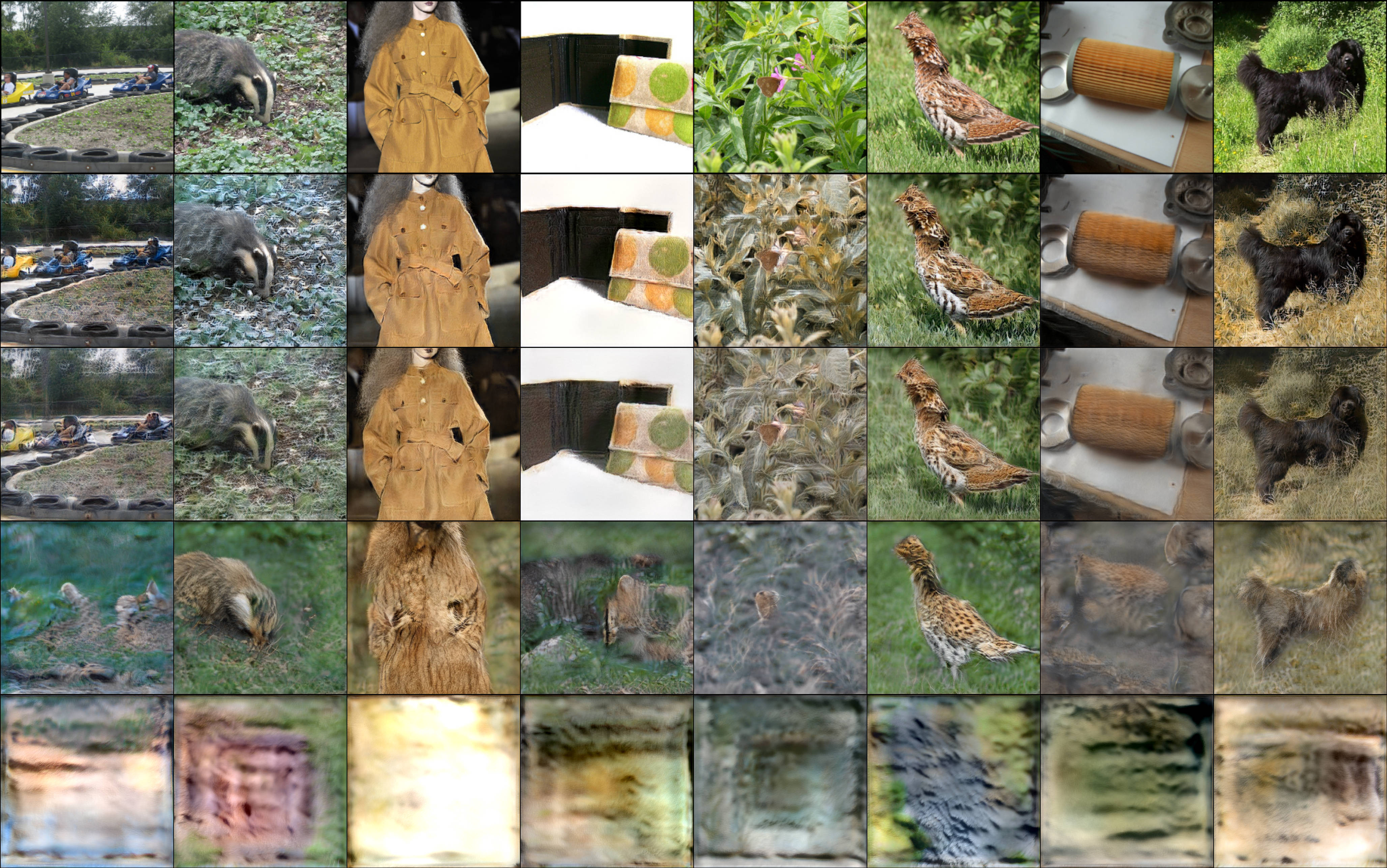
Figure 7: Samples for ImageNet.

Our method is likely to have problems when the GAN generator cannot understand the concepts of the classification or semantic segmentation network. In Figure 7, we use the 1x1 convolutional layers we have trained on the AFHQ wild data to transfer activations from ImageNet data. The top row shows the original images. The next four rows show our method’s reconstructions from Layer1 to Layer4. We can see that, especially in Layer3, the reconstructions have worse quality than samples for the AFHQ wild data, where the StyleGAN2 generator and 1x1 convolution were trained on.

5 Conclusion and Future Work

We proposed a new method to visualize activations of classification and semantic segmentation networks by stitching them with a GAN generator. We extensively evaluated our method and provided evidence that its accuracy is comparable to gradient descent methods while running about two orders of magnitude faster.

We investigated how the accuracy of the reconstructions is affected when stitching into different layers of the GAN generator. Our results show that it is a good start to stitch into a layer that has the same number of samplings distance from the output of the GAN generator, as the layer we start from in the classification or segmentation network has from the input. For 4 out of 6 layers, this choice of target layer to stitch into provided the best results. Only for Layer2 and Layer3 of the ResNet50 network, it was better to stitch into one layer closer to the output of the StyleGAN2 generator.

For future work, it would be interesting to stitch the ResNet50 classifier trained on ImageNet with a GAN that has seen roughly the same variety of concepts. Also, a weakness of the method is that the GAN generator needs to understand the concepts of the classification or segmentation network. Otherwise, the reconstructed image is further away from the original input. This weakness might, however, be utilized for out-of-distribution (OOD) detection or uncertainty estimation.

Appendix A Layer3 to Different End Layer

Figure 8 shows the GAN reconstructions when stitching from Layer3 into -2 to +2 samplings distance. The top row shows the original dataset images, the next 5 rows from top to bottom show the reconstructions for stitching into -2 to +2 samplings distance. For the AFHQ wild data we use the same noise seed (z vector) per column. For mapping into shallower layers (-1, -2 distance), the reconstruction becomes pixelated, likely due to the upsampling of the activations when transferring them into the GAN layer. For mapping into the +2 distance layer, they look fairly realistic, but have more hallucinated content, especially visible in the wolf image second from the left, which looks more like a lion there.

Figure 8: Transfer from Layer3 into -2 to +2 samplings distance.

Appendix B Layer3 Lowest Cosine Similarity Samples

Figure 9 shows the 8 images out of the 500 validation images where our GAN-based method reconstructing the activations from Layer3 had the lowest cosine similarity. It seems to have problems with sharp backgrounds (backgrounds that are in focus), and it also has problems keeping the white color of the tiger in the first and third images from the right.

Figure 9: Shows the 8 images out of the 500 validation images where our GAN-based method reconstructing the activations from Layer3 had lowest cosine similarity. Top line shows the original dataset images, bottom line our reconstructions.

Appendix C Layer3 Variations

Figure 10 and Figure 11 show 31 reconstructions from Layer3 of ResNet50 with different noise seeds (the upper left image is the original dataset image). In Figure 10, it is not always keeping the white color of the original image.

Figure 10: Variations from different noise seeds for reconstructions from Layer3. Upper left image is the original dataset image.

Figure 11: Variations from different noise seeds for reconstructions from Layer3. Upper left image is the original dataset image.

Appendix D Digipath Generator Architecture

In this section, we describe the architecture of the GAN generator we used for the experiments on the Digipath data. We use a UNet-like architecture for the generator as shown in Figure 12. The input is random Gaussian noise of a spatial size of 600x600. The content for the ”Downsample”, ”Upsample”, and ”Head” layers is shown in Figure 13. Each upsample layer has two inputs. First the input from the skip connection, which is referred to as ”Skip Input” in Figure 13. The second input comes from the upsample layer below it, or from the last downsample layer in the case of the first upsample layer. This second input is referred to as ”Input” in Figure 13. It is upsampled via nearest neighbor scaling to the spatial size of ”Skip Input”, and then in the channel dimension concatenated with it.

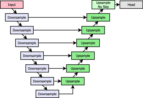
Figure 12: Architecture of the GAN generator we used for the Digipath data.

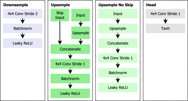
Figure 13: Layers for the GAN generator we used for the Digipath data.

References

- Bansal et al. (2021) Bansal, Y., Nakkiran, P., and Barak, B. Revisiting model stitching to compare neural representations. In Ranzato, M., Beygelzimer, A., Dauphin, Y., Liang, P., and Vaughan, J. W. (eds.), Advances in Neural Information Processing Systems, volume 34, pp. 225–236. Curran Associates, Inc., 2021. URL https://proceedings.neurips.cc/paper/2021/file/01ded4259d101feb739b06c399e9cd9c-Paper.pdf.
- Choi et al. (2020) Choi, Y., Uh, Y., Yoo, J., and Ha, J.-W. Stargan v2: Diverse image synthesis for multiple domains. In Proceedings of the IEEE Conference on Computer Vision and Pattern Recognition, 2020.
- Deng et al. (2009) Deng, J., Dong, W., Socher, R., Li, L., Kai Li, and Li Fei-Fei. ImageNet: A large-scale hierarchical image database. In 2009 IEEE Conference on Computer Vision and Pattern Recognition, pp. 248–255, 2009. doi: 10.1109/CVPR.2009.5206848.
- Dosovitskiy & T.Brox (2016) Dosovitskiy, A. and T.Brox. Inverting visual representations with convolutional networks. In IEEE Conference on Computer Vision and Pattern Recognition (CVPR), 2016. URL http://lmb.informatik.uni-freiburg.de/Publications/2016/DB16. arXiv:1506.02753.
- Gatys et al. (2015) Gatys, L. A., Ecker, A. S., and Bethge, M. A neural algorithm of artistic style, 2015. URL https://arxiv.org/abs/1508.06576.
- Goodfellow et al. (2014) Goodfellow, I., Pouget-Abadie, J., Mirza, M., Xu, B., Warde-Farley, D., Ozair, S., Courville, A., and Bengio, Y. Generative adversarial nets. In Ghahramani, Z., Welling, M., Cortes, C., Lawrence, N., and Weinberger, K. (eds.), Advances in Neural Information Processing Systems, volume 27. Curran Associates, Inc., 2014. URL https://proceedings.neurips.cc/paper/2014/file/5ca3e9b122f61f8f06494c97b1afccf3-Paper.pdf.
- He et al. (2016) He, K., Zhang, X., Ren, S., and Sun, J. Deep residual learning for image recognition. In 2016 IEEE Conference on Computer Vision and Pattern Recognition (CVPR), pp. 770–778, 2016. doi: 10.1109/CVPR.2016.90.
- Karras et al. (2020) Karras, T., Laine, S., Aittala, M., Hellsten, J., Lehtinen, J., and Aila, T. Analyzing and improving the image quality of stylegan. In 2020 IEEE/CVF Conference on Computer Vision and Pattern Recognition, CVPR 2020, Seattle, WA, USA, June 13-19, 2020, pp. 8107–8116. Computer Vision Foundation / IEEE, 2020. doi: 10.1109/CVPR42600.2020.00813. URL https://openaccess.thecvf.com/content_CVPR_2020/html/Karras_Analyzing_and_Improving_the_Image_Quality_of_StyleGAN_CVPR_2020_paper.html.
- Kingma & Ba (2015) Kingma, D. P. and Ba, J. Adam: A Method for Stochastic Optimization. In 3rd International Conference on Learning Representations, ICLR 2015, San Diego, CA, USA, May 7-9, 2015, Conference Track Proceedings, 2015.
- Lenc & Vedaldi (2015) Lenc, K. and Vedaldi, A. Understanding image representations by measuring their equivariance and equivalence. In 2015 IEEE Conference on Computer Vision and Pattern Recognition (CVPR), pp. 991–999, 2015. doi: 10.1109/CVPR.2015.7298701.
- Mahendran & Vedaldi (2014) Mahendran, A. and Vedaldi, A. Understanding deep image representations by inverting them. 2015 IEEE Conference on Computer Vision and Pattern Recognition (CVPR), pp. 5188–5196, 2014.
- Odena et al. (2016) Odena, A., Dumoulin, V., and Olah, C. Deconvolution and checkerboard artifacts. Distill, 2016. doi: 10.23915/distill.00003. URL http://distill.pub/2016/deconv-checkerboard.
- Olah et al. (2017) Olah, C., Mordvintsev, A., and Schubert, L. Feature visualization. Distill, 2017. doi: 10.23915/distill.00007. https://distill.pub/2017/feature-visualization.
- Paszke et al. (2019) Paszke, A., Gross, S., Massa, F., Lerer, A., Bradbury, J., Chanan, G., Killeen, T., Lin, Z., Gimelshein, N., Antiga, L., Desmaison, A., Köpf, A., Yang, E. Z., DeVito, Z., Raison, M., Tejani, A., Chilamkurthy, S., Steiner, B., Fang, L., Bai, J., and Chintala, S. Pytorch: An imperative style, high-performance deep learning library. In Wallach, H. M., Larochelle, H., Beygelzimer, A., d’Alché-Buc, F., Fox, E. B., and Garnett, R. (eds.), Advances in Neural Information Processing Systems 32: Annual Conference on Neural Information Processing Systems 2019, NeurIPS 2019, December 8-14, 2019, Vancouver, BC, Canada, pp. 8024–8035, 2019. URL https://proceedings.neurips.cc/paper/2019/hash/bdbca288fee7f92f2bfa9f7012727740-Abstract.html.