Challenges of cellwise outliers

Abstract

It is well-known that real data often contain outliers. The term outlier typically refers to a case, that is, a row of the $n\times d$ data matrix. In recent times a different type has come into focus, the cellwise outliers. These are suspicious cells (entries) that can occur anywhere in the data matrix. Even a relatively small proportion of outlying cells can contaminate over half the rows, which is a problem for rowwise robust methods. This article discusses the challenges posed by cellwise outliers, and some methods developed so far to deal with them. New results are obtained on cellwise breakdown values for location, covariance and regression. A cellwise robust method is proposed for correspondence analysis, with real data illustrations. The paper concludes by formulating some points for debate.

Keywords: Anomaly detection, Breakdown value, Correspondence Analysis, Multivariate statistics, Robustness.

1 Introduction

Real-world data often contains elements that do not follow the pattern suggested by the majority of the data. Such outliers may be gross errors with the potential to severely distort a statistical analysis, but they may also be valuable pieces of information that warrant further inspection. Therefore we want the ability to detect outliers, no matter what caused them.

The approach of robust statistics, as formalized by e.g. Huber (1964) and Hampel et al. (1986) has been to first obtain a robust fit, i.e. a model that fits the majority of the data well, and then to look for cases that deviate from that fit. An important assumption underlying this approach is that of casewise contamination, in which a case is either an outlier or free of any contamination. This is also called rowwise contamination, because cases are typically encoded as rows of the data matrix. Different formalizations of casewise contamination exist, but the most common one is to assume that the observed data was generated from a clean distribution $F$ with probability $1-\varepsilon>0.5$ and from an arbitrary distribution $H$ with probability $\varepsilon<0.5$. In other words, we observe $\bm{X}$ defined as

$$\bm{X}=(1-B)\bm{Y}+B\bm{Z}$$ (1)

where $B\sim\mbox{Bernoulli}(\varepsilon)$ takes on the values 0 or 1, $\bm{Y}\sim F$, $\bm{Z}\sim H$, and $B$ is independent of $\bm{Y}$ and $\bm{Z}$. This is known as the Tukey-Huber contamination model (THCM). A commonly used equivalent formulation is $\bm{X}\sim F_{\varepsilon}\coloneqq(1-\varepsilon)F+\varepsilon H$. The general goal is to estimate the characteristics of $F$ given that we only observe $F_{\varepsilon}$ and, importantly, we don’t assume anything about $H$.

With this model in mind, a wide variety of robust statistical methods has been developed for settings including the estimation of location and covariance, fitting regression models, carrying out principal component analysis and discriminant analysis, analyzing time series and so on, see for instance the books by Hampel et al. (1986), Rousseeuw and Leroy (1987), and Maronna et al. (2019).

Under the THCM model it is assumed that a case is either coming from an arbitrary distribution $H$ that may have no relation to $F$, or is a perfect draw from $F$. Therefore, methods developed under this model tend to either trust all coordinates of a case, or downweight all of them simultaneously. But there are also situations where one or more coordinates (entries, cells) of a case are suspect whereas the others are fine. By downweighting such a case entirely we may lose valuable information residing in its uncontaminated cells.

This explains why nowadays also another contamination model is being considered, that of cellwise outliers. It was first published by Alqallaf et al. (2009). They assumed that we observe a random variable $\bm{X}$ given by

$$\bm{X}=(\bm{I}-\bm{B})\bm{Y}+\bm{B}\bm{Z}$$

where $\bm{B}$ is a diagonal matrix, whose diagonal entries can only take the values zero or one. This allows some components of the observed random vector $\bm{X}$ to be contaminated, whereas others are clean. The model thus assumes that the data were initially generated by the intended distribution $F$, but afterward contaminated by replacing some cells by other values. In a given row it may happen that no cells are replaced, or a few, or even all of them. Figure 1 illustrates the difference between the casewise (rowwise) model in the left panel and the cellwise model in the right panel.

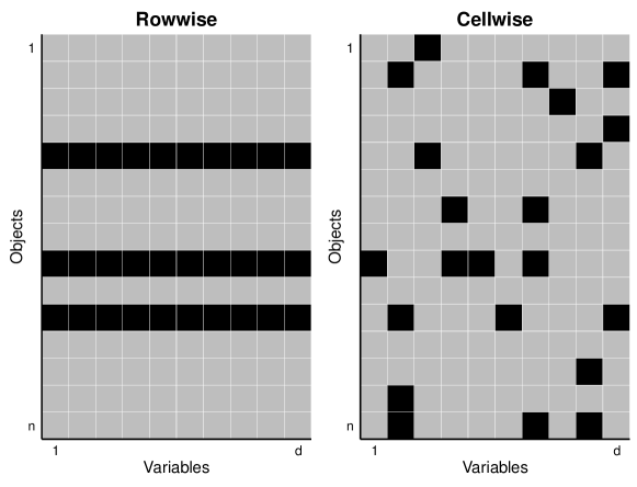
Figure 1: Rowwise outlier model (left) versus cellwise outlier model (right). Black means outlying. A small fraction of cellwise outliers can contaminate many rows.

Cellwise outliers embody a paradigm shift from rowwise outliers. Arguably the most drastic change is the fact that a small percentage of contaminated cells can contaminate a large fraction of the rows. For instance, assume that cells are contaminated with probability $\varepsilon$ and that this happens for all cells independently. In that situation the probability that a case (row) is contaminated in at least one of its cells equals

$$P[\mbox{row is contaminated}]=1-(1-\varepsilon)^{d}$$ (2)

which grows very quickly with the dimension $d$. For example, in $d=15$ dimensions a fraction $\varepsilon=0.05$ of contaminated cells suffices to have on average over $50\%$ of contaminated rows, and then the methods developed for the THCM model are no longer reliable.

Long before the notion of cellwise outliers appeared in print in Alqallaf et al. (2009), it was discussed informally by some. One of us remembers clearly that the topic was brought up in the early eighties in seminar talks by Alfio Marazzi and Werner Stahel at ETH Zürich. It was presented as an open problem, including formula (2). The general feeling then was that the tools available at that time were insufficient to address this challenge.

The remainder of our paper is organized as follows. In section 2 we give an overview of the methodology that has been developed for dealing with cellwise outliers, in various settings. In section 3 we prove some new results on cellwise breakdown values. Next, section 4 proposes the first cellwise robust method for correspondence analysis with two real data illustrations. Section 5 then evaluates the current state of research on cellwise robustness and raises some points for discussion. Section 6 concludes.

2 Methods for dealing with cellwise outliers

In this section we give an overview of methodology developed for dealing with cellwise outliers. We first treat “point clouds”, i.e. single-class multivariate numerical data. Then we discuss other models including regression, classification, principal component analysis, and clustering.

2.1 Detecting cellwise outliers

Detecting cellwise outliers turns out to be a difficult task. The most straightforward way of trying to detect cellwise outliers is to look for outliers in each variable separately. A simple approach is to robustly standardize each variable yielding a robust z-score, and then to compare these z-scores to quantiles of a reference distribution (e.g. the standard Gaussian) to decide whether or not to flag a cell. A more involved version of detecting marginal outliers is to use a univariate filter such as the one proposed by Gervini and Yohai (2002). Either way, to allow for a wider range of potentially asymmetric distributions one could first robustly transform the variables to central normality as in Raymaekers and Rousseeuw (2021c).

While flagging marginal outliers is fast, only rather extreme cellwise outliers will be identified reliably, since relations between the variables are not taken into account. For instance, consider the bivariate setting in Figure 2. Case 2 has a marginally outlying value $x_{2,2}$ , whereas case 3 has a marginally outlying $x_{3,1}$ . But for case 4 things are not so clear. The marginal approach does not see anything wrong with its $x_{4,1}$ or $x_{4,2}$ even though it is clearly an outlier relative to the pattern of the large majority of the datapoints, for which $X_{1}$ and $X_{2}$ are negatively related. This illustrates that flagging marginal outliers is insufficient in general.

Figure 2: Cellwise outliers need not be marginally outlying.

Moreover, based on Figure 2 alone it is undecidable whether case 4 has a cellwise outlier in $X_{1}$ or $X_{2}$ or maybe both. But note that it might be possible to decide whether $x_{4,1}$ or $x_{4,2}$ is a cellwise outlier if we had more variables in the data that were correlated with $X_{1}$ and $X_{2}$ . This suggests that in this particular situation the curse of dimensionality may be something of a blessing.

This idea motivates approaches for detecting cellwise outliers that consider more than just the marginal distributions. One direction is to extend the univariate GY filter of Gervini and Yohai (2002). Leung et al. (2017) extended it to a bivariate filter in the context of estimating location and covariance. More recently, Saraceno and Agostinelli (2021) went to more than two dimensions.

Another approach is the Detect Deviating Cells (DDC) algorithm of Rousseeuw and Van den Bossche (2018). This procedure uses robust simple linear regressions of each variable on other variables in the data. Combining this information yields predicted values for each cell. The difference between the original dataset and its prediction provides a residual for each cell. One can then flag cellwise outliers by large standardized cellwise residuals. This approach has received some attention, and in fact the most successful versions of the filter approach incorporate DDC in their filter. Walach et al. (2020) used a similar approach for metabolomics data by aggregating outlyingness over pairwise log-ratios.

More recently, some approaches were developed that try to go beyond combining bivariate relations by incorporating all relations in the data. Raymaekers and Rousseeuw (2021a) consider each case in turn and look for a vector parameter that captures the shift needed to bring the case into the fold. Through $L^{1}$ regularization they enforce sparsity on this shift, so that only a minority of the cells of the case are actually shifted. This algorithm is called cellHandler, and was shown to be effective in identifying complex adversarial cellwise outliers. The inputs of cellHandler are the data matrix as well as one of the robust estimates of its covariance matrix described in the next subsection.

d	Univariate GY	Bivariate GY	DDC	cellHandler
5	0.0007	0.0027	0.0005	0.0076
10	0.0012	0.0087	0.0012	0.0186
20	0.0037	0.0304	0.0033	0.0674
50	0.0059	0.1672	0.0150	0.5594

Table 1: Flagging cellwise outliers: computation times in seconds for a dataset with $n=1000$ and varying dimension $d$.

Table 1 compares the computation times of several methods for detecting cellwise outliers. The sample size was always $n=1000$ and the dimension $d$ ranged from 5 to 50. The data were generated from a Gaussian distribution with mean zero and covariance matrix $\Sigma_{jk}=(-0.9)^{|j-k|}$ in which 10% of the cells were replaced by the value 5. All computations were carried out in R, and the reported times are averages over 10 replications. As expected the univariate filter is the fastest. The bivariate GY filter takes more time, also compared to DDC. The cellHandler method is the slowest in relative terms but still fast.

As there are several approaches for detecting cellwise outliers, some guidance is useful to select one of them in a given situation. When there are reasons to assume that all cellwise outliers are marginally outlying, a univariate filter is sufficient. When they are expected to stand out in bivariate plots one can e.g. use the bivariate GY filter (Leung et al., 2017). However, for less computational effort one might as well run DDC, which combines information from many variables and provides predicted values for the flagged cells. Also cellHandler does that. In order to choose between the latter pair, it is good to know that cellHandler requires a robust covariance estimate which assumes $n>p$, and also assumes a roughly elliptical data shape. DDC does not make these assumptions and is faster, but when it is applicable cellHandler is more accurate for detecting complex outliers.

A somewhat related approach is the SPADIMO algorithm by Debruyne et al. (2019). It is not purely cellwise because it starts by identifying outlying cases by large robust distances from a casewise robust location and covariance matrix. Next, it tries to identify the cells responsible for the outlyingness of those cases. For this it uses regularized regression to identify sparse directions of maximal outlyingness.

2.2 Estimating location and covariance

If there is any reassuring news in the study of cellwise outliers, it is probably that multivariate location can still be estimated reliably from a robustness viewpoint by combining robust location estimates on the marginals. The typical example is the coordinatewise median, given by

$$\bm{\hat{\mu}}(\bm{X})=(\operatorname*{\mbox{median}}_{i=1}^{n}x_{i1},\ldots,\operatorname*{\mbox{median}}_{i=1}^{n}x_{id})$$ (3)

for a dataset $\bm{X}$ with $n$ rows and $d$ columns. While such a componentwise estimate of location may not always have the most desirable properties, it is at least consistent under general conditions and very robust. The same is true for the estimation of the scales of the variables, in other words, the diagonal of a covariance matrix.

However, when we leave the comfort zone of estimating multivariate location and componentwise scale, things become much more challenging. For cellwise robust estimation of a covariance matrix, Van Aelst et al. (2011) proposed the cellwise Stahel-Donoho estimator. This is an extension of the casewise Stahel-Donoho covariance estimator (Stahel, 1981; Donoho, 1982). It was seen to perform reasonably well under casewise contamination, but in the setting of cellwise contamination it is now outperformed by more recent methods, as illustrated in Figure 1 of Agostinelli et al. (2015) and Figure 9 of Rousseeuw and Van den Bossche (2018).

Danilov (2010) thoroughly studied the approach of filtering the data before estimating a covariance matrix. He considered the three-step procedure of (i) detecting the contaminated cells, (ii) processing them in some way to reduce their influence, and (iii) estimating the location and the covariance matrix. For the detection, he looked at marginal approaches based on robust z-scores, as well as multivariate approaches based on partial Mahalanobis distances. He ended up proposing the latter with the caveat that the computation time scales exponentially with the dimension $d$ if one wants to identify cellwise outliers in all possible subspaces. For processing the outlying cells he compared winsorizing, censoring, and setting them to missing. The final proposal used a multivariate cell detection method and then set the outlying cells to missing, followed by the MLE for the resulting incomplete dataset. Continuing in this direction, the two-step generalized S-estimator (2SGS) was proposed by Agostinelli et al. (2015) and extended by Leung et al. (2017). This was the best performer for a number of years. The 2SGS method combines a bivariate filter with the generalized S-estimator for missing data (Danilov et al., 2012), and is implemented in the R-package GSE (Leung et al., 2019).

Recently there have been new attempts at estimating the covariance matrix under adversarial cellwise outliers. Raymaekers and Rousseeuw (2021a) proposed an iterative approach of (i) running cellHandler to flag outlying cells, (ii) setting these cells to missing, and (iii) applying the EM algorithm to re-estimate the covariance matrix. While this approach performs quite well, it is purely algorithmic in nature without a tractable objective function, and therefore its properties are difficult to analyze. However, building on these ideas Raymaekers and Rousseeuw (2022b) proposed a cellwise robust version of the well-known casewise robust minimum covariance determinant (MCD) estimator of Rousseeuw (1984). The new cellMCD method does optimize an objective function and was proven to possess a high breakdown value under cellwise contamination. Its algorithm iterates a kind of C-steps, which (like those for the casewise MCD) always lower the objective function. Therefore the algorithm is guaranteed to converge to a solution, which may be a local minimum. The initial estimator uses a combination of the robust correlation estimator of Raymaekers and Rousseeuw (2021b) and DDC, but several initial estimates could be used. The methods described in this paragraph are implemented in the R package cellWise (Raymaekers and Rousseeuw, 2022a).

d	Classical	MCD	S	2SGS	cellMCD
5	0.0000	0.0423	0.1448	0.5730	0.2403
10	0.0002	0.0950	0.3145	1.6476	0.3733
20	0.0002	0.3065	1.0548	15.206	1.3153
50	0.0015	2.0049	8.0532	213.02	24.770

Table 2: Estimation of location and covariance: computation times in seconds for a dataset with $n=1000$ and varying dimension $d$.

Table 2 lists the computation times of the classical mean and covariance matrix, as well as those of the casewise robust MCD and S-estimators. These are compared to the cellwise robust methods 2SGS and cellMCD. The setup was the same as for Table 1, with all methods run in R in their default version. We note that the cellwise robust methods take the most time, but are still feasible. The 2SGS method was the slowest, partly due to its default initial estimator that could be replaced by a different one.

Rousseeuw (2023) recently proposed a method to statistically analyze data with cellwise weights, and implemented it for the estimation of location and covariance. One possible application is to first assign weights to cells depending on how outlying they are (e.g. based on a standardized residual), and then to compute a reweighted location and covariance matrix by cellwise weighted maximum likelihood.

2.3 Estimating a precision matrix

In many applications it is the inverse of the covariance matrix, also known as the precision matrix, that is of main interest. In low dimensions, it is of course possible to estimate a covariance matrix and then to invert the estimate, but this is no longer the case in high dimensions because the estimated covariance matrix is often singular. Rather than regularizing the covariance matrix, one can then estimate the precision matrix and regularize it at the same time. This induces zeroes in the precision matrix, which correspond to partial correlations of zero which in turn correspond to conditional independence in the Gaussian graphical model. One of the most popular estimators of a high-dimensional precision matrix is the graphical lasso of Friedman et al. (2008). It requires the input of an estimate of the covariance matrix $\bm{\widehat{\Sigma}}$, usually the classical empirical covariance. The precision matrix $\bm{\Theta}$ is then estimated as

$$\bm{\hat{\Theta}}=\operatorname*{\mbox{argmin}}_{\bm{\Theta}\succcurlyeq 0}\left(\operatorname{\mbox{trace}}\left(\bm{\widehat{\Sigma}}\bm{\Theta}\right)-\log(\det(\bm{\Theta}))+\lambda\sum_{j\neq\ell}|\bm{\Theta}_{j\ell}|\right)\;.$$ (4)

A natural question is whether a robust version of $\bm{\widehat{\Sigma}}$ would result in a robust precision matrix estimator, and this is indeed the case. This idea has been studied empirically and theoretically by Öllerer and Croux (2015), Croux and Öllerer (2016), Tarr et al. (2016), Loh and Tan (2018), and Katayama et al. (2018), using different $\bm{\widehat{\Sigma}}$ based on robust pairwise correlations. The $\bm{\widehat{\Sigma}}$ in these studies are typically of the form

$$\bm{\widehat{\Sigma}}_{j\ell}=\mbox{s}\!\left(\bm{X}_{.j}\right)\mbox{s}\!\left(\bm{X}_{.\ell}\right)\mbox{r}\!\left(\bm{X}_{.j},\bm{X}_{.\ell}\right)$$ (5)

where $\mbox{s}(\cdot)$ denotes a robust scale estimator, often the $Q_{n}$ estimator of Rousseeuw and Croux (1993), and $\mbox{r}(\cdot)$ denotes a robust correlation estimator such as Spearman’s rank correlation. Note that $\bm{\widehat{\Sigma}}$ needs to be positive semidefinite for (4) to work. When $\bm{\widehat{\Sigma}}$ is not positive semidefinite it is first modified, e.g. by adding a small multiple of the identity matrix. The resulting precision matrix estimators perform well under non-adversarial cellwise contamination, are fast to compute, and can be analyzed theoretically due to the well-defined objective function (4). But since they focus on pairwise correlations, their performance is likely to suffer under more adversarial cellwise outliers.

2.4 Regression

Regression in the presence of cellwise outliers has mainly been studied in the linear model with numerical predictors and response. More precisely, we model the observed pairs $(\bm{x}_{1},y_{1}),\ldots,(\bm{x}_{n},y_{n})$ where $\bm{x}_{i}$ is a $p\times 1$ vector for $i=1,\ldots,n$ as

$$y_{i}=\alpha+\bm{\beta}\bm{x}_{i}+\mbox{noise}_{i}$$ (6)

where the regression coefficients $\alpha$ and $\bm{\beta}=(\beta_{1},\ldots,\beta_{p})$ need to be estimated.

In casewise robust linear regression, an observed pair $(\bm{x}_{i},y_{i})$ is considered to be either outlying or entirely clean. For cellwise robust regression the setup is different. It remains true that the response $y_{i}$ is either outlying or clean because it is univariate, so it has only one cell. The main difference lies in the contamination of the predictor variables. Instead of working with either outlying or entirely clean $\bm{x}_{i}=(x_{i1},\ldots,x_{ip})$, we now allow for some of the cells $x_{ij}$ to be contaminated while the others are clean. We would like to use the clean cells of $\bm{x}_{i}$ in the estimation of $\alpha$ and $\bm{\beta}$, but at the same time limit the harmful influence of the bad cells of $\bm{x}_{i}$ .

One of the earliest proposals for cellwise robust regression is the shooting S-estimator of Öllerer et al. (2016). It uses the coordinate descent algorithm (Bezdek et al., 1987), also called “shooting algorithm”. If we fit only the $j$-th slope coefficient $\beta_{j}$ while keeping the other slopes fixed at their previous values, we can do

$$y_{i}^{(j)}\sim\;\hat{\alpha}_{j}^{\mbox{\tiny{new}}}+\hat{\beta}_{j}^{\mbox{\tiny{new}}}x_{ij}\;\;\;\;\;\mbox{ where }\;\;\;\;\;y_{i}^{(j)}\coloneqq y_{i}-\bm{\hat{\beta}}_{-j}^{\mbox{\tiny{old}}}\bm{x}_{i,-j}\;\;.$$ (7)

This can be seen as a simple regression of a new response $\bm{y}^{(j)}$ on the $j$-th predictor. The shooting S-estimator makes two changes to the coordinate descent algorithm. The first is that in the simple regression (7) the OLS regression is replaced by a casewise robust S-estimator. The second is that the response $\bm{y}^{(j)}$ is ‘robustified’ in each iteration, to make sure the cellwise outliers don’t propagate to the new responses in the iteration steps. Bottmer et al. (2022) recently proposed a version of shooting S regression for high dimensions which uses hard thresholding, yielding sparse estimates of the regression coefficients.

An alternative proposal was made by Leung et al. (2016). Their model assumes joint multivariate normality of the pairs $(\bm{x}_{i},y_{i})$ before the cells are contaminated. They start by estimating the location $\bm{\hat{\mu}}$ and covariance matrix $\bm{\widehat{\Sigma}}$ of the joint distribution of the pairs $(\bm{x}_{i},y_{i})$ by the 2SGS estimator of Agostinelli et al. (2015), with a modified filter in the first step. Then the slope coefficients and the intercept are estimated from $\bm{\hat{\mu}}$ and $\bm{\widehat{\Sigma}}$ by the usual formulas

$$\bm{\hat{\beta}}:=\bm{\widehat{\Sigma}}_{xx}^{-1}\bm{\widehat{\Sigma}}_{xy}\;\;\;\mbox{ followed by }\;\;\;\hat{\alpha}=\hat{\mu}_{y}-\bm{\hat{\mu}}_{x}^{{\bm{\top}}}\bm{\hat{\beta}}\;.$$ (8)

The robustness of this estimator stems from the 2SGS method, which is known to perform quite well in many situations. On the other hand, this approach requires the covariance matrix to be invertible so it is not applicable to higher-dimensional settings that the shooting S version of Bottmer et al. (2022) can handle.

p	Classical	LTS	S	Shooting S
5	0.0008	0.0442	0.0440	0.5525
10	0.0011	0.0720	0.0947	1.1577
20	0.0018	0.1558	0.3650	3.2820
50	0.0034	0.8009	1.7363	12.417

Table 3: Linear regression: computation times in seconds for a dataset with $n=1000$ and $p$ regressors.

Table 3 shows the computation times of several regression methods, using the same setup as in Tables 1 and 2. The classical least squares regression is compared to the casewise robust Least Trimmed Squares regression (Rousseeuw, 1984) and S regression (Rousseeuw and Yohai, 1984), and to the cellwise robust shooting S method of Öllerer et al. (2016). The latter is the slowest but still quite feasible, even though its computation is in pure R. The proposal of Leung et al. (2016) is not shown because its computation time is that of the 2SGS method in Table 2, the additional computation being very quick.

An interesting approach was introduced by Agostinelli and Yohai (2016) for the more general problem of robust estimators for linear mixed models. They propose a composite estimator which minimizes the scales of Mahalanobis distances on pairs of variables. The use of pairwise Mahalanobis distances makes this approach more robust against cellwise outliers than casewise S-estimators. It would be interesting to evaluate the robustness of this approach against adversarial cellwise outliers.

The proposal of Filzmoser et al. (2020) starts from a casewise robust method such as MM-regression. Then SPADIMO (Debruyne et al., 2019) is applied to the flagged cases in the hope of identifying the cells responsible for their outlyingness. Next, these flagged cells are imputed by nearest neighbors applied to the unflagged cells, and the imputed data is used to update the residuals of the regression. Finally, casewise weights are obtained from the standardized residuals, and used in a weighted least squares regression to obtain updated regression coefficients. This three-step procedure is iterated. As the algorithm relies on a casewise robust initial estimator, it cannot be cellwise robust in a general sense. However, it is possible that cellwise robustness could be obtained by replacing the initial estimator.

Finally, we mention some recent related proposals. Su et al. (2021) first compute a robust covariance matrix of the joint distribution of the pairs $(\bm{x}_{i},y_{i})$. For this they use a method based on pairwise correlations as mentioned above, using the approach of Gnanadesikan and Kettenring (1972) or the Gaussian rank correlation studied by Boudt et al. (2012). They then plug the square root of this covariance matrix into the adaptive lasso objective to obtain variable selection. Toka et al. (2021) propose a three-step procedure consisting of (i) identifying marginal cellwise outliers using robust z-scores and setting them to missing, (ii) running the casewise robust MCD estimates of location and covariance on the complete cases, and then imputing the NA’s as in the E-step of the EM algorithm, and (iii) applying a robust lasso regression to the imputed data. Saraceno et al. (2021) carry out robust seemingly unrelated regressions using several univariate MM-regressions, and apply the 2SGS method of Agostinelli et al. (2015) to the residual matrix. For regression with compositional covariates, Štefelová et al. (2021) propose a four-step procedure: (i) detecting outlying cells by DDC, (ii) imputing the outlying cells that are not in outlying rows, (iii) running rowwise robust regression on the imputed data, and (iv) performing inference based on multiple imputation.

We end the section with a brief discussion. While there have been several approaches to cellwise robust regression, there is still much room for further research. First, not much attention has been devoted to outlier detection so far. For casewise robustness, there is a taxonomy of outlier types based on whether $\bm{x}_{i}$ or the residual of $y_{i}$ is outlying, or both, see Rousseeuw and van Zomeren (1990). The detection of such casewise outliers depends crucially on having a reliable robust fit $(\hat{\alpha},\bm{\hat{\beta}})$. But in many of the existing proposals, cellwise outliers are detected in a kind of pre-processing step, and the robust fit is not yet used to detect them. Second, with few exceptions, most of the proposals do not yet have provable robustness guarantees, such as a high breakdown value under cellwise contamination. This may be due to the lack of a natural framework such as those for casewise robust regression, or it may be due to the general complexity of dealing with cellwise outliers.

2.5 Principal component analysis

Principal component analysis (PCA) is an essential tool of multivariate statistics. Several formulations of classical PCA exist, e.g. based on the spectral decomposition of the covariance matrix or the singular value decomposition of the centered data matrix. One way of looking at it is that PCA approximates the dataset $\bm{X}$ with $d$ columns by a new dataset $\bm{\widehat{X}}$ that lies in a $q$-dimensional affine subspace of dimension $q<d$ such that the Frobenius norm $||\bm{X}-\bm{\widehat{X}}||_{F}$ is minimized. Several proposals exist for casewise robust PCA, including spherical PCA (Locantore et al., 1999), PCA based on least trimmed squares orthogonal regression (Maronna, 2005), the PCAgrid projection pursuit method (Croux et al., 2007), and the hybrid ROBPCA method (Hubert et al., 2005). There are also approaches for casewise robust sparse PCA, see Croux et al. (2013), Hubert et al. (2016), and Wang and Van Aelst (2020).

For cellwise outliers, things are more difficult. One complication stems from the fact that classical PCA projects the data orthogonally on a lower dimensional subspace. Projecting a case (row) with cellwise outliers is problematic, as the outlying cells can propagate over all cells. Therefore, whenever the algorithm makes a projection, the outlying cells should be addressed.

An early proposal for the related problem of cellwise robust factor analysis was made by Croux et al. (2003). The first cellwise robust PCA method was proposed by Maronna and Yohai (2008). Instead of minimizing the Frobenius norm of $||\bm{X}-\bm{\widehat{X}}||_{F}$ they minimize a robust approximation error by applying a bounded function $\rho$ to each cell of $\bm{X}-\bm{\widehat{X}}$ and summing the resulting errors. The minimization is carried out by iteratively solving weighted least squares problems. The bounded $\rho$ function guarantees that a single cell cannot dominate the approximation error. A different proposal for cellwise robust PCA was made by She et al. (2016). The MacroPCA method proposed by Hubert et al. (2019) aims to be an all-in-one method capable of handling missing values as well as being robust to cellwise and rowwise outliers. It starts from DDC and incorporates elements of ROBPCA. It imputes cells that caused data points to lie far from the fitted subspace, and produces cellwise residuals that can be plotted.

d	Classical	ROBPCA	PCAgrid	MacroPCA
10	0.0043	0.1091	0.2216	0.1551
50	0.0161	0.2414	1.8707	0.4163
100	0.0413	0.3641	4.0087	0.9460
500	1.0227	2.9865	22.727	12.142
1000	3.3084	8.6023	56.335	13.778

Table 4: PCA: computation times in seconds for a dataset with $n=1000$ and dimension $d$.

The computation times of several of these PCA methods are shown in Table 4. The setup was the same as in Tables 1 to 3, but going up to higher dimensions $d$. The task was to compute the first 10 components. The casewise robust ROBPCA and PCAgrid methods take more time than classical PCA but are still fast enough. The MacroPCA method is slower than ROBPCA but faster than PCAgrid, illustrating that cellwise robust PCA is computationally affordable.

2.6 Clustering

Several methods for clustering data with cellwise outliers have been proposed. The earliest was Farcomeni (2014), who used a mixture model with an additional $n\times d$ parameter matrix of zeroes and ones, indicating which cells should be flagged and set to missing. The goal was to maximize the observed likelihood of the unflagged cells. The method was implemented in the R package snipEM (Farcomeni and Leung, 2019) which is no longer maintained. García-Escudero et al. (2021) consider a model in which clusters are linear, i.e. they lie near lower-dimensional subspaces. Each cluster is then fitted by a cellwise robust PCA in the style of Maronna and Yohai (2008) discussed above. They minimize the robust scales of the coordinatewise residuals as in least trimmed squares regression. The algorithm iterates the following three steps: (i) updating the subspace parameters by robust PCA, (ii) updating the weights indicating which cells are deemed outlying, and (iii) updating the group memberships, similar to the usual k-means clustering algorithm.

2.7 Time series

We are not aware of existing work on applying cellwise robust methods to time series, but we will describe a setting in which they prove useful, the fitting of autoregressive models. Suppose we have a univariate time series $y_{t}$ for $t=1,\ldots,n$. The autoregressive model AR($p$) of order $p$ then assumes that

$$y_{t}=\beta_{1}y_{t-1}+\ldots+\beta_{p}y_{t-p}+\varepsilon_{t}$$

for $t=p+1,\ldots,n$ where the $\varepsilon_{t}$ are i.i.d. according to a Gaussian distribution with mean zero and standard deviation $\sigma$. For simplicity we assume that the model has no intercept term. Note that there are $n-p$ complete sets $(y_{t},y_{t-1},\ldots,y_{t-p})$ which can be combined as successive rows in an $(n-p)\times(p+1)$ matrix $\bm{Z}$. The AR($p$) model can thus be seen as a linear model with the first column of $\bm{Z}$ as response and the other columns as regressors, and various classical methods exist to estimate the parameter vector $\bm{\beta}=(\beta_{1},\ldots,\beta_{p})$ from $\bm{Z}$. The simplest of these is just the LS regression estimator, sometimes called ‘naive OLS’ in this context.

Now consider an outlying value $y_{t}$ . In the AR($p$) model it will occur $p+1$ times: once as response, and once in each of the $p$ lags. In other words, one outlying $y_{t}$ affects $p+1$ rows of $\bm{Z}$, each time in a single cell. Since the breakdown value of any affine equivariant regression method is at most $0.5$, using such a method in this setting has a breakdown value of at most $1/(2p+2)$ which can be unpleasantly low. (And if the original series is first differenced, e.g. to remove a seasonal effect, this upper bound is cut in half again.) The odds against robust estimation of $\bm{\beta}$ are thus stacked. For a discussion of this issue and a review of the literature on types of outliers in AR($p$) models see Section 7.2 of Rousseeuw and Leroy (1987).

This is a setting where cellwise robust methods can shine. As an illustration, we generated an AR(3) time series with parameters $\bm{\beta}=(0.5,\,0.2,\,0.2)$, $\sigma=1$ and length $n=1000$. We then created a kind of ‘day of the week effect’ by replacing every 7th entry $y_{t}$ by the outlying value 10. (The R script generating the data and the subsequent analysis is available from the webpage https://wis.kuleuven.be/statdatascience/robust/papers-2020-2029). The original time series thus has 14% of outliers, but they contaminate 569 rows of $\bm{Z}$ out of 997, so 57% of them. The classical estimate of $\bm{\beta}$ becomes $(0.11,0.11,0.08)$ which is far from $(0.5,\,0.2,\,0.2)$, and the estimate of the error standard deviation $\sigma=1$ is 3.79 . Casewise robust regression does not work here either, with LTS yielding $\bm{\hat{\beta}}=(0.73,0.02,0.01)$ and $\hat{\sigma}=1.85$, and the default MM regression in R giving $\bm{\hat{\beta}}=(0.14,0.14,0.12)$ and $\hat{\sigma}=1.72$ . Fortunately, cellwise robust methods do give good results. The regression method of Leung et al. (2016) first computes a robust covariance matrix $\bm{\widehat{\Sigma}}$ of $\bm{Z}$ by 2SGS and then applies (8), yielding $\bm{\hat{\beta}}=(0.52,0.21,0.17)$. Moreover, from $\hat{\sigma}^{2}=\bm{\widehat{\Sigma}}_{yy}-\bm{\hat{\beta}}^{\bm{\top}}\bm{\widehat{\Sigma}}_{xx}\bm{\hat{\beta}}$ one obtains $\hat{\sigma}=0.96$. Applying the same formulas to the cellMCD covariance matrix gives similar results, with $\bm{\hat{\beta}}=(0.53,0.18,0.19)$ and $\hat{\sigma}=0.92$ .

To conclude, the autoregressive model can by its nature create many outlying cells, which handicap casewise robust methods whereas cellwise robust methods can deal with them.

2.8 Various other settings

Aerts and Wilms (2017) construct a cellwise robust version of linear and quadratic discriminant analysis. To this end they estimate a cellwise robust precision matrix for each class as in Croux and Öllerer (2016), and plug these into the assignment rule. Further work could deal with the situation that new data points to be classified may also contain outlying cells.

In functional data analysis, a case is not a row of a matrix but a function such as a curve. In that setting, cellwise outliers correspond to local deviations (like spikes) in a curve, rather than global outlyingness of the entire curve. In the taxonomy of Hubert et al. (2015) of functional outliers these are called isolated outliers, and methods have been constructed to detect them. García-Escudero et al. (2021) apply cellwise robust methods to functional data.

3 Breakdown values

The breakdown value plays an important role in the study of casewise robust methods, because a positive breakdown value is a necessary condition for robustness. In several models, natural equivariance properties imply an upper bound of 50% on the breakdown value, and methods have been developed that get close to this upper bound.

In the setting of cellwise robustness, Alqallaf et al. (2009) define the asymptotic cellwise breakdown value of a location estimator. Here we will focus on finite-sample breakdown values in the sense of Donoho and Huber (1983) and Lopuhaä and Rousseeuw (1991). Below we will study two statistical models of practical importance, and show that under some conditions that appear natural at first sight it is impossible to obtain a high cellwise breakdown value.

3.1 Breakdown of location and covariance estimators

Consider a finite sample consisting of $n$ data points in $d$ dimensions, denoted by its $n\times d$ data matrix $\bm{X}$. We want to estimate its unknown location vector by the estimator $\bm{\hat{\mu}}$. Then we define the finite-sample cellwise breakdown value of $\bm{\hat{\mu}}$ at $\bm{X}$ as the smallest fraction of cells per column that need to be replaced to carry the estimate outside all bounds. Formally, denote by $\bm{X}^{m}$ any corrupted sample obtained by replacing at most $m$ cells in each column of $\bm{X}$ by arbitrary values. Then the finite-sample cellwise breakdown value of the location estimator $\bm{\hat{\mu}}$ at $\bm{X}$ is given by

$$\varepsilon^{*}_{n}(\bm{\hat{\mu}},\bm{X})=\min\left\{\frac{m}{n}:\;\sup_{\bm{X}^{m}}{\left|\left|\bm{\hat{\mu}}(\bm{X}^{m})-\bm{\hat{\mu}}(\bm{X})\right|\right|}=\infty\right\}.$$ (9)

This is a natural finite-sample version of the asymptotic cellwise breakdown value defined by Alqallaf et al. (2009).

Let us start with a trivial remark. If an estimator has an upper bound on its casewise breakdown value, then that upper bound also holds for its cellwise breakdown value. Indeed, a contaminated dataset obtained by replacing $m$ cases by other cases can also be created by replacing the cells of the replaced cases by those of the replacing cases, which affects $m$ cells in each column. Therefore (9) is at most $\lfloor(n+1)/2\rfloor/n$ for any translation equivariant location estimator due to Theorem 2.1 of Lopuhaä and Rousseeuw (1991).

We will see that some conditions that appear natural imply a rather low cellwise breakdown value. One such condition is

$$\mbox{if all points of }\bm{X}\mbox{ lie in a lower-dimensional}$$ (10)

$$\mbox{ affine subspace, then }\bm{\hat{\mu}}(\bm{X})\mbox{ lies in that subspace as well.}$$

This is a very weak exact fit property, which nevertheless restricts the breakdown value as shown by the following result.

Proposition 1.

The cellwise breakdown value of any location estimator $\bm{\hat{\mu}}$ satisfying (10) is bounded by

$$\varepsilon^{*}_{n}(\bm{\hat{\mu}},\bm{X})=\left\lceil\frac{n}{d}\right\rceil/n\,\approx\frac{1}{d}$$ (11)

at any dataset $\bm{X}$.

The proof uses the fact that the data can be moved to a hyperplane by replacing no more than $\lceil n/d\rceil$ cells in each variable. All proofs of this section can be found in the Appendix.

Alqallaf et al. (2009) prove an upper bound on the asymptotic cellwise breakdown value of a location estimator that also goes to zero like $1/d$. For this they require two conditions. One of these is the so-called $\delta$-consistency of the estimator. The other is affine equivariance of $\bm{\hat{\mu}}$, which says that for all $d\times 1$ vectors $\bm{v}$ and all $d\times d$ nonsingular matrices $\bm{A}$ it holds that

$$\bm{\hat{\mu}}(\bm{v}\bm{1}_{d}^{\bm{\top}}+\bm{X}\bm{A})=\bm{v}+\bm{A}^{\bm{\top}}\bm{\hat{\mu}}(\bm{X})$$ (12)

where $\bm{1}_{d}$ is the $d\times 1$ vector of ones. In words, the estimator is equivariant for translations and linear transformations. The transposed $\bm{A}^{\bm{\top}}$ in (12) is due to the fact that $\bm{X}$ contains the data points as rows, not columns.

Our result is more general, in that we do not need $\delta$-consistency, and instead of affine equivariance we can use orthogonal equivariance. This is a weaker form of equivariance which only requires (12) for orthogonal matrices $\bm{A}$.

Corollary 1.

Any orthogonally equivariant location estimator satisfies property (10), and hence the upper bound of Proposition 1 applies.

All this illustrates that orthogonal equivariance, and even the weaker condition (10), are unpromising properties for location estimators that want to be cellwise robust. But for location, one can easily avoid this problem by combining coordinatewise robust location estimates.

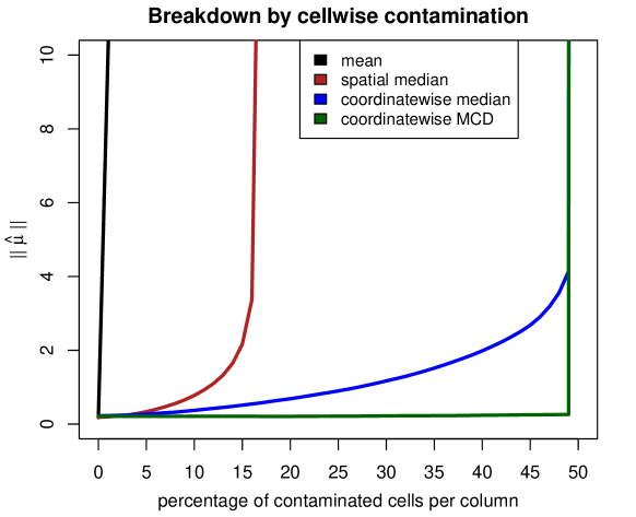
Figure 3: Empirical illustration of breakdown due to cellwise contamination, for $n=100$ cases in $d=4$ dimensions.

We provide a simple empirical illustration. The experiment went as follows. First $n=100$ points were generated from the standard Gaussian distribution in $d=4$ dimensions. These have $k=0$ outlying cells per column. Next, the number of outlying cells per column was incremented in steps of 1 such that the cases with outlying cells overlap as little as possible, so when $k=25$ all cases have one outlying cell. The outlying cells were all given the value 500. On each contaminated dataset the following location estimators were run: the arithmetic mean, the spatial median which minimizes $\sum_{i=1}^{n}||\bm{x}_{i}-\bm{\hat{\mu}}||$, the coordinatewise median (3), and the coordinatewise univariate MCD estimator. Figure 3 plots the euclidean norm $||\bm{\hat{\mu}}||$ of each estimator as a function of the percentage of contaminated cells per column. It shows the averaged norms over 200 replications. The horizontal axis ends at 50%, corresponding to the upper bound on the breakdown value of translation equivariant estimators.

In Figure 3 we see that the mean is the first to move far away. In fact, if we would let $n$ go up and the value of every outlying cell go from 500 to infinity, the line of the mean would become vertical, since 1 cellwise outlier per column is enough for breakdown. In contrast, the norm of the spatial median stays low for a long time before going up. (In fact, for exactly the fraction $1/d=25\%$ of outlying cells per column the spatial median attains norm 250, because then all datapoints lie near the hyperplane $x_{1}+x_{2}+x_{3}+x_{4}=500$.) Note that the spatial median is not affine equivariant but it is orthogonally equivariant, so Corollary 1 applies.

The coordinatewise median escapes the upper bound $1/d$ because it does not satisfy the condition (10). Indeed, Rousseeuw and Leroy (1987) already gave a simple counterexample (on page 250) where the coordinatewise median lies outside the hyperplane whenever $d>2$. (For $d\leqslant 2$ the bound is trivially satisfied.) Since the median of each variable only breaks down when the variable has 50% or more outlying values, the same holds when these separate medians are combined in (3). The reasoning is the same for combining the univariate MCD estimates of each coordinate.

Cellwise robust covariance estimation is harder than location. Estimators $\bm{\widehat{\Sigma}}$ of a covariance (scatter) matrix can break down in two ways. Analogously to the casewise setting, we can define the cellwise explosion breakdown value of the covariance estimator $\bm{\widehat{\Sigma}}$ as

$$\varepsilon^{+}_{n}(\bm{\widehat{\Sigma}},\bm{X})=\min\left\{\frac{m}{n}:\;\sup_{\bm{X}^{m}}\lambda_{1}(\bm{\widehat{\Sigma}})=\infty\right\}$$ (13)

where $\lambda_{1}$ denotes the largest eigenvalue. Moreover, we define the cellwise implosion breakdown value of $\bm{\widehat{\Sigma}}$ as

$$\varepsilon^{-}_{n}(\bm{\widehat{\Sigma}},\bm{X})=\min\left\{\frac{m}{n}:\;\inf_{\bm{X}^{m}}\lambda_{d}(\bm{\widehat{\Sigma}})=0\right\}$$ (14)

where $\lambda_{d}$ is the smallest eigenvalue. Implosion is just as bad as explosion, since a singular covariance matrix is not invertible so one cannot compute Mahalanobis distances, carry out discriminant analysis, and so on.

Also in this setting, a good cellwise breakdown value is harder to obtain than its casewise counterpart. For instance, the casewise implosion breakdown value of the classical covariance matrix at a typical dataset is very high, in fact it is $(n-d)/n\approx 1$. This is because whenever $d+1$ of the original data points are kept, the classical covariance remains nonsingular. In stark contrast, its cellwise implosion breakdown value is quite low. This even holds for all covariance estimators that satisfy the following intuitive condition analogous to (10):

$$\mbox{if all points of }\bm{X}\mbox{ lie in a lower-dimensional}$$ (15)

$$\mbox{affine subspace, then }\bm{\widehat{\Sigma}}(\bm{X})\mbox{ is singular.}$$

Proposition 2.

The cellwise implosion breakdown value of any covariance estimator $\bm{\widehat{\Sigma}}$ satisfying (15) is bounded by

$$\varepsilon^{-}_{n}(\bm{\widehat{\Sigma}},\bm{X})=\left\lceil\frac{n-1}{d}\right\rceil/n\,\approx\frac{1}{d}$$ (16)

for any dataset $\bm{X}$.

This result appears to be new, and it is also implied by equivariance. Recall that a covariance estimator $\bm{\widehat{\Sigma}}$ is affine equivariant if for all $d\times 1$ vectors $\bm{v}$ and all $d\times d$ nonsingular matrices $\bm{A}$ it holds that

$$\bm{\widehat{\Sigma}}(\bm{v}\bm{1}_{d}^{\bm{\top}}+\bm{X}\bm{A})=\bm{A}^{\bm{\top}}\bm{\widehat{\Sigma}}(\bm{X})\bm{A}\;.$$ (17)

Corollary 2.

Any affine equivariant covariance estimator $\bm{\widehat{\Sigma}}$ satisfies property (15), and hence the upper bound of Proposition 2 applies.

The upper bound $\lceil(n-1)/d\rceil/n\approx 1/d$ in Corollary 2 is a lot lower than that inherited from the casewise breakdown value of affine equivariant covariance estimators, which is $\lfloor(n-d+1)/2\rfloor/n\approx 0.5$ . The fact that implosion breakdown can happen easily in the cellwise setting was not mentioned in the literature before. For the cellwise robust covariance estimators of Öllerer and Croux (2015), only their explosion breakdown value was stated. The above results make it useful to rule out implosion by a prior constraint like $\lambda_{d}(\bm{\widehat{\Sigma}})\geqslant a$, or from a formulation in which $\bm{\widehat{\Sigma}}$ is a convex combination of two matrices, one of which is the identity matrix with a small coefficient. Both approaches would be at odds with affine equivariance, but here we are in the cellwise setting. This mechanism has also been employed in casewise settings without affine equivariance, see e.g. Ollila and Tyler (2014).

Note that in spite of the above negative results it is possible to construct estimators of covariance that achieve a higher cellwise breakdown value, as in Raymaekers and Rousseeuw (2022b). Their proposal for a cellwise robust MCD estimator attains a breakdown value of $(n-h+1)/n$ where $h$ can be as low as $\lfloor n/2\rfloor+1$ but is recommended to be chosen as $h=0.75n$. It can thus reach an asymptotic breakdown value of $0.5$, which is the highest possible.

3.2 Breakdown in regression

For linear regression we use the model (6) but write it a little differently as

$$\bm{y}=\bm{X}\bm{\gamma}+\mbox{noise}$$ (18)

where $\bm{y}=(y_{1},\ldots,y_{n})$ is the $n\times 1$ column vector of responses, and the rows of $\bm{X}$ are of the form $(1,\bm{x}_{i}^{\bm{\top}})$. The $(p+1)\times 1$ vector $\bm{\gamma}=(\alpha,\beta_{1},\ldots,\beta_{p})^{\bm{\top}}$ combines the intercept and the slopes. We also combine the actual data (that is, everything but the first column of $\bm{X}$ which is constant) in the $n\times(p+1)$ matrix $\bm{Z}$ whose $i$-th row is $(x_{i1},\ldots,x_{ip},y_{i})$.

We now contaminate the dataset $\bm{Z}$. By $\bm{Z}^{m}$ we mean any corrupted set of covariates obtained by replacing at most $m$ cells in each column of $\bm{Z}$ by arbitrary values. We define the finite-sample cellwise breakdown value of the regression estimator $\bm{\widehat{\gamma}}$ at the dataset $\bm{Z}$ as

$$\varepsilon^{*}_{n}(\bm{\widehat{\gamma}},\bm{Z})=\min\left\{\frac{m}{n}:\;\sup_{\bm{X}^{m}}{\left|\left|\bm{\widehat{\gamma}}(\bm{Z}^{m})-\bm{\widehat{\gamma}}(\bm{Z})\right|\right|}=\infty\right\}.$$ (19)

Many existing regression methods $\bm{\widehat{\gamma}}$ satisfy the following intuitive property:

$$\mbox{if }y_{i}=\bm{x}_{i}^{\bm{\top}}\bm{\gamma}_{0}\mbox{ for all $i=1,\ldots,n$ and }\bm{X}\mbox{ is not}$$ (20)

$$\mbox{in a lower-dimensional}\mbox{ subspace, then }\bm{\widehat{\gamma}}=\bm{\gamma}_{0}\;.$$

The condition that $\bm{X}$ does not lie in a lower-dimensional vector subspace serves to avoid multicollinearity, which causes problems for many regression methods.

Proposition 3.

The cellwise breakdown value of any regression estimator $\bm{\widehat{\gamma}}$ satisfying (20) is bounded by

$$\varepsilon^{*}_{n}(\bm{\widehat{\gamma}},\bm{X},\bm{y})\leqslant\left\lceil\frac{n-1}{p+1}\right\rceil/n\,\approx\frac{1}{p+1}$$ (21)

at any dataset $\bm{Z}$.

Also the weak condition (20) is satisfied under natural equivariance properties. The first of these is regression equivariance, which requires that for all $(p+1)\times 1$ vectors $\bm{v}$ it holds that

$$\bm{\widehat{\gamma}}(\bm{X},\bm{y}+\bm{X}\bm{v})=\bm{\widehat{\gamma}}(\bm{X},\bm{y})+\bm{v}$$ (22)

for all datasets $(\bm{X},\bm{y})$. This intuitive condition is similar to translation equivariance for location estimators. The second property is scale equivariance, meaning that for any constant $c$ we have

$$\bm{\widehat{\gamma}}(\bm{X},c\,\bm{y})=c\,\bm{\widehat{\gamma}}(\bm{X},\bm{y})\;.$$ (23)

We do not even need affine equivariance, which says that $\bm{\widehat{\gamma}}(\bm{X}\bm{A},\bm{y})=\bm{A}^{-1}\bm{\widehat{\gamma}}(\bm{X},\bm{y})$ for all nonsingular matrices $\bm{A}$.

Corollary 3.

Any estimator $\bm{\widehat{\gamma}}$ that is regression equivariant (22) and scale equivariant (23) satisfies property (20), and hence the upper bound of Proposition 3 applies.

We could easily write down analogous results for implosion of the scale estimator of the noise term.

In conclusion, if we want a regression estimator with a better cellwise breakdown value we have to let go of the natural combination of equivariance properties (22) and (23), and even of the intuitive condition (20). When working with high-dimensional data we are used to penalizations that cause the regression to deselect some of the covariates, but even for lower-dimensional data one may have to resort to such techniques, or novel ones.

4 Cellwise robust correspondence analysis

In this section we present the first cellwise robust method for correspondence analysis.

4.1 Classical correspondence analysis

Correspondence analysis (CA) was proposed by Hirschfeld (1935) and further developed by Benzécri et al. (1973) as a method for analyzing categorical data that can be represented by a contingency table. The main aim is to construct a so-called biplot, a bivariate plot summarizing part of the structure in the contingency table. This biplot can be thought of as analogous to plotting the first two principal components of continuous numerical data.

Let $\bm{X}$ be an $n\times d$ contingency table of counts $x_{ij}$ with $i=1,\ldots,n$ and $j=1,\ldots,d$. Denote by $N=\sum_{i=1}^{n}\sum_{j=1}^{d}\bm{X}_{ij}$ the sum of all counts in $\bm{X}$, and let $\bm{P}=\bm{X}/N$ be the matrix of relative frequencies. Denote by $\bm{r}$ the $n\times 1$ column vector containing the sums of the rows of $\bm{P}$ , and by $\bm{c}$ the $d\times 1$ vector containing the sums of its columns. Also write $\bm{D}_{\bm{r}}=\operatorname{\mbox{diag}}(\bm{r})$ and $\bm{D}_{\bm{c}}=\operatorname{\mbox{diag}}(\bm{c})$. Finally, let $\bm{R}=\bm{D}_{\bm{r}}^{-1}\bm{P}$ be the matrix of standardized row profiles, for which each row sums to 1. Correspondence analysis is based on the matrix of weighted centered row profiles

$$\bm{S}:=\bm{D}_{\bm{r}}^{1/2}\left(\bm{R}-\bm{1}_{d}\bm{c}^{\bm{\top}}\right)\bm{D}_{\bm{c}}^{-1/2}$$ (24)

where $\bm{1}_{d}$ is the $d\times 1$ column vector of ones. Note that each row of $\bm{1}_{d}\bm{c}^{\bm{\top}}$ also sums to one, so the row totals of $\bm{R}-\bm{1}_{d}\bm{c}^{\bm{\top}}$ are all zero. This implies that the columns of $\bm{R}-\bm{1}_{d}\bm{c}^{\bm{\top}}$ are linearly dependent, and therefore $\bm{S}$ is not of full rank either.

From here on, $\bm{S}$ is treated as if it were a dataset with continuous variables (columns). Since $\bm{S}$ is singular by construction, it is useful to carry out its singular value decomposition, yielding

$$\bm{S}=\bm{U}\bm{\Gamma}\bm{V}^{\bm{\top}}\,.$$ (25)

Here $\bm{U}$ contains the left singular vectors in its orthogonal columns, $\bm{\Gamma}$ is a diagonal matrix with the singular values on the diagonal, and $\bm{V}$ contains the right singular vectors in its orthogonal columns. If we denote the rank of $\bm{S}$ by $k$, the matrix $\bm{U}$ is $n\times k$, $\bm{\Gamma}$ is $k\times k$, and the loadings matrix $\bm{V}$ is $d\times k$ . Using this singular value decomposition we can now represent the rows as well as the columns of the data set $\bm{S}$ . The principal coordinates of the rows are given by $\bm{D}_{\bm{r}}^{-1/2}\bm{U}\bm{\Gamma}$, and those of the columns are given by $\bm{D}_{\bm{c}}^{-1/2}\bm{V}\bm{\Gamma}$. In a biplot we only show the first two coordinates of both.

4.2 Cellwise robust CA

In order to construct a cellwise robust correspondence analysis method, we need a robust version of the singular value decomposition (25) of $\bm{S}$. For this purpose we construct a modification of the cellwise robust MacroPCA method of Hubert et al. (2019). Its original version fits the PCA model

$$\bm{S}=\bm{1}_{n}\bm{\mu}^{\bm{\top}}+\bm{T}\bm{V}^{\bm{\top}}+\mbox{noise}$$ (26)

where $\bm{\mu}$ is the center, the matrix of scores $\bm{T}$ is $n\times k$, and the loadings matrix $\bm{V}$ is $d\times k$. The noise has the same dimensions as $\bm{S}$. In this context the choice of $k$, the number of principal components, is important. This is because a point is considered outlying when its orthogonal distance to the fitted subspace is high, so if the maximal $k$ were chosen all points would be in the subspace and none would be considered outlying. This also implies that the loadings are not nested, that is, the loading columns for $k=2$ are not a subset of those for $k=3$. MacroPCA selects $k$ as the smallest number of components that explains at least 80% of the variability.

Since our goal is to fit the model (25), we have added an option to MacroPCA which fixes the center $\bm{\mu}$ beforehand rather than estimating it from the data. For our current purpose we fix $\bm{\mu}$ at zero, so the first term of (26) disappears. Let us denote the estimated loadings and scores by $\bm{\widehat{V}}$ and $\bm{\widehat{T}}$. For the singular values in the diagonal matrix $\bm{\widehat{\Gamma}}$ we take the square root of $n$ times the eigenvalues estimated by MacroPCA. Finally, we compute $\bm{\widehat{U}}=\bm{\widehat{T}}\bm{\widehat{\Gamma}}^{-1}$. The combination of the resulting matrices $\bm{\widehat{U}}$, $\bm{\widehat{\Gamma}}$ and $\bm{\widehat{V}}$ provides a robust version of the decomposition (25). Using these matrices, the biplot can be drawn as before.

To illustrate this approach to cellwise robust correspondence analysis we consider two examples studied previously by Riani et al. (2022) in the context of casewise robust correspondence analysis.

4.3 Correspondence analysis of the clothes data

The first example is a contingency table containing trade flows of clothes from outside the European Union into each of its 28 member states (the data is from before 2020, so the United Kingdom was still included). The columns in the contingency table in Riani et al. (2022) are five different price brackets, from lowest to highest. The contingency table $\bm{X}$ is thus of size $28\times 5$, as are the matrices $\bm{P}$ and $\bm{S}$.

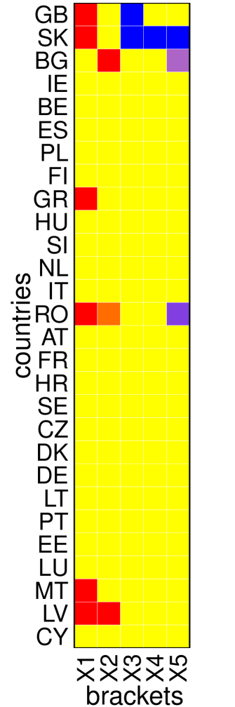
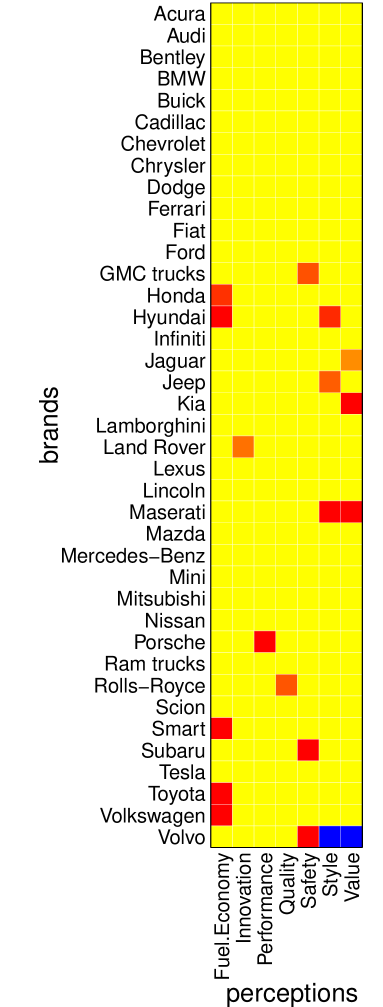
Figure 4: Cellmap showing the result of DetectDeviatingCells (DDC) on the clothes data (left) and on the brands data (right).

As an initial exploration of the data, we start by applying DDC to $\bm{S}$. (Note that we should not apply DDC to the original contingency table $\bm{X}$ because the scales of its rows are not comparable, as they are correlated with the population size of their countries.) The DDC algorithm yields a predicted data matrix $\bm{\widehat{S}}$, and thus also cellwise residuals $\bm{S}-\bm{\widehat{S}}$. The left panel of Figure 4 shows the DDC cellmap of the clothes data, which graphically represents the standardized cellwise residuals. Red cells indicate standardized residuals above $\sqrt{\chi^{2}_{1,0.99}}\approx 2.57$, with the intensity of the color increasing with the actual residual. Such cells have a higher value than predicted. Blue cells indicate standardized residuals below $-\sqrt{\chi^{2}_{1,0.99}}$ , so their value was lower than predicted. The majority of the cells, shown in yellow, are roughly in line with their predicted values.

The cellmap draws our attention to a few unusual trade flows. In particular, the United Kingdom (with country code GB), Slovakia (SK), Greece (GR), Romania (RO), Malta (MT) and Latvia (LV) import many clothes of the lowest price segment, compared to what would be expected based on their other trade flows. These results can be interpreted. For instance, it is known that the United Kingdom imports large quantities of very cheap clothing from Bangladesh, India and China. Also Slovakia imports a lot from these countries, and judging from its blue cells it imports relatively few clothes from the upper three segments.

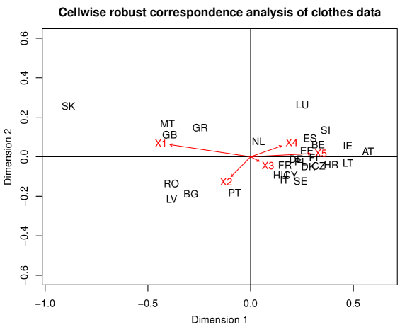
Figure 5: Biplot of the clothes data based on the proposed cellwise robust fit.

Next, we apply the zero-center version of MacroPCA to $\bm{S}$, yielding a robust loadings matrix $\bm{\widehat{V}}$, scores $\bm{\widehat{T}}$, and estimated eigenvalues. From these we derive $\bm{\widehat{\Gamma}}$ and $\bm{\widehat{U}}=\bm{\widehat{T}}\bm{\widehat{\Gamma}}^{-1}$. Using $\bm{\widehat{U}}$, $\bm{\widehat{\Gamma}}$ and $\bm{\widehat{V}}$ yields the biplot in Figure 5. We see that SK is outlying on the left and loads very strongly onto the category of the lowest price bracket $X_{1}$ , whereas it lies in the opposite direction of the variables $X_{3}$, $X_{4}$ and $X_{5}$ corresponding with the three highest price brackets. We also note the small group of countries MT, GB, GR that lie in the direction of the lowest bracket $X_{1}$ , and the countries RO, LV, BG in the direction of the two lowest brackets $X_{1}$ and $X_{2}$ . The countries on the right spend more on the higher brackets. Overall, this biplot looks quite similar to the casewise robust biplots in Figure 4 of Riani et al. (2022).

4.4 Correspondence analysis of the brands data

The second example is a contingency table summarizing the 2014 Auto Brand Perception survey by Consumer Reports (USA), which is publicly available on https://boraberan.wordpress.com/2016/09/22/. The survey questioned 1578 participants on what they considered attributes of 39 different car brands. The list of possible attributes consisted of Fuel Economy, Innovation, Performance, Quality, Safety, Style, and Value. Respondents had to select all the characteristics from the list which they felt applied to a brand. The resulting contingency table $\bm{X}$ is thus of size $39\times 7$, so the matrix $\bm{S}$ has the same dimensions.

We again start by applying DDC to $\bm{S}$ in order to flag outlying cells. The resulting cellmap is in the right panel of Figure 4, and reveals some interesting insights. We see that Volvo is quite exceptional in that as many as three of its cells are flagged. Its Safety perception is higher than predicted, whereas Style and Value are lower than would be expected from its other characteristics. Hyundai and Maserati have two flagged cells. Hyundai has rather high Fuel Economy and Style given its other characteristics, and Maserati seems to have exceptionally high Style and Value. (One wonders whether sometimes ‘Value’ was interpreted as ‘expensive’ rather than ‘value for money’.) Then there are another 12 cases with a single cellwise outlier. Examples are GMC trucks with high perceived Safety, Porsche with high Performance, and Toyota and Volkswagen with high Fuel Economy. In total, 15 out of the 39 brands have at least one cell flagged by DDC. The total number of flagged cells is 19, so only 7% of all cells, but they affect close to 40% of the cases. Still, a casewise robust analysis with a high-breakdown method can work here since over 50% of the cases have no outlying cells.

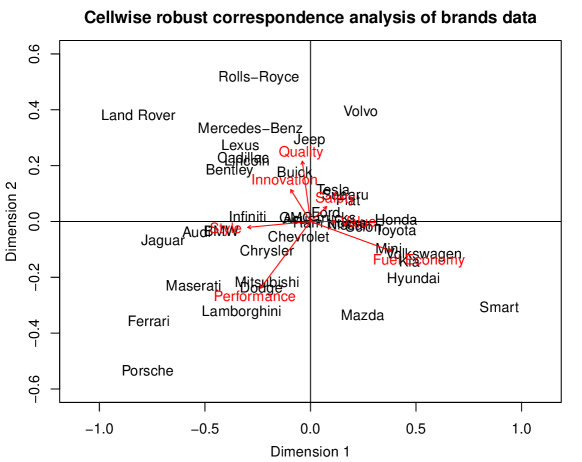
Figure 6: Biplot of the brands data based on the proposed cellwise robust fit.

Figure 6 shows the biplot based on the cellwise robust MacroPCA method. It is rather similar to that obtained by Riani et al. (2022), and both robust fits are quite different from the classical correspondence analysis shown in their Figure 6. We see some intuitively explainable structure in Figure 6. Volvo is often considered one of the safest car brands, and indeed lies in the direction of the Safety attribute. There is a collection of sports cars (Ferrari, Maserati, Lamborghini, Porsche) lying far in the direction of the Performance arrow. Rolls-Royce and Mercedes-Benz lie in the directions of Innovation and Quality, and Smart, Hyundai, and Volkswagen load heavily on Fuel Economy.

5 Discussion and challenges

In this section we put forward some points for debate, and discuss open challenges for the development of theory and methods to deal with cellwise outliers.

5.1 Interpretation of outliers as cellwise or casewise

The notions of casewise and cellwise outliers raise some questions of interpretation. On the one hand, the terms casewise contamination and cellwise contamination have a clear meaning as generative models, i.e. as recipes for different ways to create outliers. Many researchers have used these models to set up simulation studies.

On the other hand, when faced with incoming data, inferring whether an unusual row is a casewise outlier (i.e. generated by a different mechanism from the majority of the cases) or a mostly clean row with some outlying cells, is often an unidentifiable problem. As an illustration, consider a toy example from Raymaekers and Rousseeuw (2021a). Assume the clean data is i.i.d. from the 4-dimensional standard Gaussian distribution $F=N(\bm{0},\bm{I})$ and consider the row $(10,0,0,0)$. From the casewise point of view, this case is “equivalent” to the row $(\sqrt{50},\sqrt{50},0,0)$, and to the row $(5,5,5,5)$, as both can be obtained by an orthogonal transformation of the data, under which the distribution $N(\bm{0},\bm{I})$ remains the same. But from the cellwise point of view, one would conclude that the first row has one cellwise outlier, the second has 2 and the last has 4. Therefore, the conclusions depend on whether we adopt the casewise or the cellwise paradigm.

While a data-based determination of casewise versus cellwise outliers may not be feasible, it may be not necessary to make such a distinction from the viewpoint of estimation. In his Section 4.1, Danilov (2010) states that “Detection methods for cellwise contamination can be used to disarm casewise outliers if the covariance structure is known well enough to identify them. If we remove several cells from a casewise outlier so that the remaining sub-vector is not outlying any more, its influence on the covariance estimate is significantly reduced and can be tolerated.” This viewpoint seems sensible to us. But in order to efficiently disarm adversarial casewise outliers, one would need a rather accurate fit (covariance estimate) when looking for the most harmful cells. Pairwise correlation methods are likely to suffer substantially under adversarial casewise outliers, and thus may have to be combined by some method targeting casewise outliers as well, like 2SGS. It does seem like the “disarming” approach can work. When applying the cellwise MCD estimator to all the benchmark datasets in the robustbase R package (Maechler et al., 2022) that were previously analyzed by casewise robust methods, the fits turned out to be quite similar (Raymaekers and Rousseeuw, 2022b).

An alternative view is that, in the cellwise world, we can consider something a casewise outlier when too many cells are flagged or need to be changed in order to bring the case into the fold. This idea has been used as an algorithmic tool in the 2SGS method, where cases get downweighted as a whole in the GSE step, and in the MacroPCA method. As a way to interpret the results it has also been implemented in DDC, which has a rule to flag rows that contain much cellwise outlyingness. There it is a kind of post-processing step. Nevertheless one should remain conscious of the fact that this viewpoint does not quite match the generative models of rowwise and cellwise outliers, unless one assumes a model that generates both. Several authors have indeed generated data with both types of outliers combined.

5.2 Insights from sparsity

Robustness considerations have recently received increasing attention in the computer science and electrical engineering communities. One particularly popular approach to casewise robustness is to take an existing objective function and then to add a penalty term about a parameter vector which encodes outliers. The estimated parameter vector thereby becomes sparse, corresponding to a low number of flagged outliers. To the best of our knowledge, the first reference to this idea is Sardy et al. (2001) who drew a parallel between using a Huber loss function in regression and penalizing a shift parameter $\bm{\delta}=(\delta_{1},\ldots,\delta_{n})$ with an $L^{1}$ penalty. In particular, they showed that minimizing

$$\sum_{i=1}^{n}\left(y_{i}-\bm{\beta}\bm{x}_{i}-\delta_{i}\right)^{2}+\lambda\sum_{i=1}^{n}{|\delta_{i}|}$$ (27)

over $\bm{\beta}$ and $\bm{\delta}$ gives the same $\bm{\hat{\beta}}$ as minimizing

$$\sum_{i=1}^{n}\rho_{\mbox{\tiny Huber},\lambda}\left(y_{i}-\bm{\beta}\bm{x}_{i}\right)\;.$$ (28)

This approach was also followed by McCann and Welsch (2007), Laska et al. (2009) and Li (2013), and was further developed by She and Owen (2011) who formulated general connections with M-estimation in robust statistics. They showed that non-convex penalties on $\bm{\delta}$ lead to more robust estimators, in the same way that M-estimators with non-convex loss functions can be more robust than M-estimators with convex loss functions. In spite of this fact, still more research gets published for convex than for non-convex penalties and loss functions, because convex functions are easier for proving theorems and writing algorithms.

A similar approach can be applied to cellwise outliers. Instead of an $n$-variate vector of shifts $\bm{\delta}$, one can use an $n\times d$ matrix $\bm{\Delta}$ of shifts to describe cellwise outliers, and penalize $\bm{\Delta}$ to make it sparse. In the context of low-rank matrix completion, this was done by Zhou et al. (2010) and Candès et al. (2011). The context is not the same as ours because of two main reasons. First, their approach is presented for PCA but it is equivariant to transposing the data matrix, whereas in the robust statistical literature on PCA there can be rowwise outliers, e.g. fully contaminated rows, but fully contaminated columns are not allowed because they would make the loadings unidentifiable. A more fundamental difference is that their approach does not aim for robustness against adversarial contamination but instead assumes that the contaminated cells occur at random positions according to the uniform distribution, and independently of each other and the clean data. This assumption is why they have no need for a non-convex penalty, in fact they use the $L^{1}$ penalty. Their method has received a lot of attention and performs well under their assumptions if the outliers do not have large orthogonal distances to the true low-rank subspace (She et al., 2016).

For regression, one could use an analogous approach by the minimization

$$\operatorname*{\mbox{argmin}}_{\bm{\beta},\bm{\Delta}}\left(\sum_{i=1}^{n}\left(y_{i}-\bm{\beta}(\bm{x}_{i}-\bm{\Delta}_{i,\cdot})\right)^{2}+\lambda\mathcal{P}(\bm{\Delta})\right)$$ (29)

where $\mathcal{P}(\cdot)$ denotes a penalty on the cells in $\bm{\Delta}$. Zhu et al. (2011) have proposed a similar idea with the convex Frobenius norm as penalty, i.e. $\mathcal{P}(\cdot)=||\cdot||_{F}$. This is designed to work when the matrix of shifts is dense but bounded, but less suitable for a sparse set of potentially gross cellwise outliers. Chen et al. (2013) go further in this direction. Like She and Owen (2011) they conclude that approaches based on convex optimization cannot be robust to casewise or cellwise outliers in the covariates. Instead they work with trimmed inner products.

For the estimation of a covariance matrix one also could try an approach similar to (29). It would be natural to minimize the negative Gaussian loglikelihood of the shifted data as in

$$\operatorname*{\mbox{argmin}}_{\bm{\mu},\bm{\Sigma},\bm{\Delta}}\left(\sum_{i=1}^{n}{\left(\log|\bm{\Sigma}|+(\bm{x}_{i}-\bm{\Delta}_{i,\cdot}-\bm{\mu})^{\bm{\top}}\bm{\Sigma}^{-1}(\bm{x}_{i}-\bm{\Delta}_{i,\cdot}-\bm{\mu})\right)}+\lambda\mathcal{P}(\bm{\Delta})\right)$$ (30)

where $\mathcal{P}(\cdot)$ again denotes a penalty on the elements of $\bm{\Delta}$. While this optimization can be carried out quite efficiently, we have found that it leads to a bias which shrinks the estimated covariance matrix. The cellwise MCD of Raymaekers and Rousseeuw (2022b) is a further development of this approach. Rather than penalizing a matrix $\bm{\Delta}$ of shifts, it penalizes an $n\times d$ matrix $\bm{W}$ with zeroes and ones that indicate which cells to include in the estimation. The objective function then becomes the observed likelihood of the incomplete dataset formed by the included cells. This avoids the bias in the estimated covariance matrix.

5.3 Models for cellwise outliers

Alqallaf et al. (2009) provided a formalization of the idea of cellwise outliers, aimed at replacing the casewise Tukey-Huber contamination model (THCM) of (1). More precisely, they assumed that we observe a random variable generated by

$$\bm{X}=(\bm{I}-\bm{B})\bm{Y}+\bm{B}\bm{Z}$$ (31)

where $\bm{B}$ is a diagonal matrix whose diagonal elements can only take on the values zero or one. To be precise, they assume $\bm{B}=\operatorname{\mbox{diag}}(B_{1},\ldots,B_{d})$ with Bernoulli distributed $B_{j}\sim\mbox{Bernoulli}(\varepsilon)$. Alqallaf et al. (2009) refer to this as the independent contamination model (ICM) but one has to be a little careful with this name, because the word independent does not refer to statistical independence, it merely means that the diagonal elements of $\bm{B}$ are allowed to differ from each other. As Alqallaf et al. (2009) point out, the THCM can be recovered from (31) by imposing the equality $B_{1}=\cdots=B_{d}$, and then the $B_{1},\ldots,B_{d}$ are not statistically independent. At the other extreme is the situation where $B_{1},\ldots,B_{d}$ are, in fact, statistically independent. If on top of that we also assume that $\bm{B}$ is independent of $\bm{Y}$ and $\bm{Z}$, we arrive at what they call the fully independent contamination model (FICM). Under the FICM each cell has a probability of $\varepsilon$ to be contaminated, and whether a cell gets contaminated does not depend on the value of the clean $\bm{Y}$ or the contamination $\bm{Z}$.

Despite the fact that developing methods that work under the FICM model is already hard, we would like to point out that FICM is a restrictive model that could be extended substantially, as already mentioned by Alqallaf et al. (2009). Recall that a random vector $\bm{X}$ following the FICM can be written as in (31) where $\bm{Y}$ follows some clean distribution $F$ and $\bm{Z}$ follows an unspecified distribution $H$. Importantly, $B_{1},\ldots,B_{d},\bm{Y},\bm{Z}$ are assumed independent. One could argue that this independence assumption is rather strong. Furthermore, in most empirical studies so far, the outlying cells have been generated with the additional assumption that also the components of $\bm{Z}$ are independent of each other, and often even constant. This leads to cells that are marginally outlying, and can thus in principle be detected by looking at the marginal distributions of the variables.

Under the casewise THCM model of (1) it is typically assumed that $B$ is independent of $\bm{Y}$, i.e. whether a case is sampled from the contaminated distribution does not depend on the value of the clean data. In general no assumptions on $H$ are made, but in simulations $H$ sometimes depends on the distribution $F$ of the clean data. For instance, for covariance estimation, one often generates outlying cases in the direction of the last eigenvector of the true covariance matrix of $F$, which is typically the most adversarial choice.

The FICM model could be extended in an analogous way. As in THCM, we do not want $\bm{B}$ to depend on $\bm{Y}$. But the values of $\bm{Z}$ could depend on $\bm{B}$ and on the distribution $F$ of the variable $\bm{Y}$. This is what happens in the structural (adversarial) cellwise outlier generation in Raymaekers and Rousseeuw (2021a, 2022b). There the diagonal entries of $\bm{B}$ are independently drawn from $\mbox{Bernoulli}(\varepsilon)$. Next, the contaminated cells are computed from the last eigenvector of the covariance matrix of the distribution of $\bm{Y}$ restricted to the variables with $B_{j}=1$. This uses the distribution of $\bm{Y}$, but not the value of $\bm{Y}$ itself.

These dependencies can be characterized by the directed acyclic graph

where $\mathcal{B}$ is the multivariate distribution of $\bm{B}$. The final observed $\bm{X}$ is at the bottom. Note that there is an arrow from the distribution $F$ to $\bm{Z}$, but not from the value $\bm{Y}$ to $\bm{Z}$. We feel that this model comes closest to the philosophy that has been dominant in the THCM setting. This model allows for much more challenging cellwise outliers than have been predominantly considered so far. On the other hand, it is a valid question whether such outliers are actually common in practice. In order to answer this question we need appropriate methods to detect them.

5.4 Cellwise outliers and heavy tails

We feel it is important to stress the difference between the contamination model (31) and the concept of heavy tails. Heavy-tailed distributions are typically defined as probability distributions whose tails are not exponentially bounded, such as the Cauchy distribution. Methods for heavy-tailed data have received a lot of attention recently, e.g. by Fan et al. (2021) who avoid the ubiquitous sub-Gaussian restriction. But note that in this context there is no notion of adversarial contamination or structured outliers.

While heavy-tailed distributions may often generate samples that appear as though they could have been generated from (31), there is a crucial difference. If the marginal distributions of an observed random vector follow a heavy-tailed distribution, the cells that seem outlying still carry information about the underlying distribution. In contrast, under the model (31) we don’t want to assume anything about the distribution of $\bm{Z}$, so we cannot use $\bm{Z}$ to obtain information on the characteristics of the distribution of $\bm{Y}$, which is the one of interest. Therefore cells generated by $\bm{Z}$ do not carry information on $\bm{Y}$. In the cellwise contamination model we should thus strive to eliminate the effect of $\bm{Z}$. If we were told which cells were generated from $\bm{Z}$, then our best bet would be to discard them and to continue with the remaining cells.

As a simple example, consider a univariate dataset with a single far out value. If we knew for a fact that the data came from a Cauchy distribution, then we should keep this unusual value and calculate the MLE for the Cauchy distribution. If, instead, we knew that the data came from a Gaussian distribution except for the suspicious value that came from some other distribution, we should discard it and perform the Gaussian MLE on the remaining values.

In spite of the two different models and objectives, there may still be merit in combining ideas from both worlds. In general, we expect that estimators for heavy-tailed data can still perform reasonably well under cellwise contamination. This may at least give them a role as initial estimators for iterative algorithms intended for data that may contain cellwise outliers.

6 Conclusion

Cellwise outliers provide a fascinating but tough challenge for statistical data analysis. Here we have reviewed some methodology that has been developed for detecting cellwise outliers and estimating location and covariance, and for carrying out a number of other tasks such as regression and PCA. From Tables 1 to 4 we conclude that computation time is not an obstacle to the use of cellwise robust methods. We showed that the cellwise breakdown values of estimators of location, covariance and regression are rather low when holding on to some intuitive notions, meaning that one has to search in new directions. We next proposed a cellwise robust approach for correspondence analysis. Finally, we discussed various issues that serve as food for thought and may inspire debate and further research.

Software availability. The code for the cellwise robust correspondence analysis method described in section 4 is available in the R package cellWise (Raymaekers and Rousseeuw, 2022a), with a vignette Correspondence_analysis_examples reproducing Figures 4 to 6.

Acknowledgment. Thanks go to Mia Hubert for interesting discussions.

Appendix

Here we give the proofs of the breakdown results in section 3.

Proof of Proposition 1.

Consider a hyperplane $H$ given by the equation $\bm{x}^{\bm{\top}}\bm{1}_{d}=c$ where $\bm{1}_{d}$ is the $d\times 1$ vector of ones, and $c$ is chosen large enough so that all data points $\bm{x}_{i}$ satisfy $\bm{x}_{i}^{\bm{\top}}\bm{1}_{d}<c$. So $\bm{X}$ lies on one side of $H$, and $H$ is not parallel to any coordinate axis. In each row of $\bm{X}$ we can then replace a single cell such that all of the resulting points lie on $H$, yielding the contaminated dataset $\bm{X}^{m}$ . We can do this by replacing no more than $\lceil n/d\rceil$ cells in each variable, which is a fraction $\lceil n/d\rceil/n$ of its $n$ cells. From property (10) it then follows that $\bm{\hat{\mu}}(\bm{X}^{m})$ lies on $H$ too. Since we can choose the value $c$ arbitrarily large, $\bm{\hat{\mu}}(\bm{X}^{m})$ breaks down. ∎

Proof of Corollary 1.

Consider a dataset $\{\bm{x}_{i};\;i=1,\ldots,n\}$ that lies on a hyperplane $H$. Then the $\bm{x}^{\prime}_{i}=\bm{x}_{i}-\bm{x}_{1}$ lie on the shifted hyperplane $H_{0}$ which passes through the origin. Now take an orthogonal matrix $\bm{U}$ which maps $H_{0}$ to the hyperplane spanned by the first $d$ orthonormal basis vectors. This maps the data points to $\bm{\widetilde{x}}_{i}=\bm{U}\bm{x}^{\prime}_{i}$. Now take the orthogonal matrix $\bm{V}=\mbox{diag}(1,\ldots,1,-1)$. By orthogonal equivariance we then obtain $\bm{\hat{\mu}}(\{\bm{V}\bm{\widetilde{x}}_{i}\})=\bm{V}(\bm{\hat{\mu}}(\{\bm{\widetilde{x}}_{i}\})).$ But $\{\bm{V}\bm{\widetilde{x}}_{i}\}=\{\bm{\widetilde{x}}_{i}\}$ hence $\bm{\hat{\mu}}(\{\bm{\widetilde{x}}_{i}\})=\bm{V}(\bm{\hat{\mu}}(\{\bm{\widetilde{x}}_{i}\}))$ so its last coordinate must be zero. Therefore $\bm{\hat{\mu}}(\{\bm{x}_{i}\})=\bm{U}^{\bm{\top}}\bm{\hat{\mu}}(\{\bm{\widetilde{x}}_{i}\})+\bm{x}_{1}$ lies on $H$, which proves (10). ∎

Proof of Proposition 2.

When $n\leqslant d$ all points of $\bm{X}$ lie on a lower-dimensional affine subspace, so (15) implies that $\lambda_{d}(\bm{\widehat{\Sigma}}(\bm{X}))=0$ so $m=0$ already suffices for breakdown. From here on we can assume $n>d$. Pick one row of the dataset, and consider an affine hyperplane that is not parallel to any coordinate axis. In the remaining $n-1$ rows we can then replace a single cell such that all of the resulting points lie on the same hyperplane, yielding the contaminated dataset $\bm{X}^{m}$ . We can do this by replacing no more than $\lceil(n-1)/d\rceil$ cells in each variable, which is a fraction $\lceil(n-1)/d\rceil/n$ of its $n$ cells. From the exact fit property (15) it then follows that $\lambda_{d}(\bm{\widehat{\Sigma}}(\bm{X}^{m}))=0$, so we obtain implosion. ∎

Proof of Corollary 2.

Consider a dataset $\bm{\widetilde{X}}$ in a lower-dimensional subspace. Let us shift and rotate $\bm{\widetilde{X}}$ so that its image $\bm{Y}$ lies in the hyperplane through the origin $\bm{0}$ spanned by the first $d-1$ orthonormal basis vectors. By affine equivariance of $\bm{\widehat{\Sigma}}$ it follows that $\bm{C}:=\bm{\widehat{\Sigma}}(\bm{Y})$ has the same eigenvalues as $\bm{\widehat{\Sigma}}(\bm{\widetilde{X}})$. We now split up $C$ in blocks of sizes $d-1$ and 1, and consider the following matrix $\bm{A}$:

$$\begin{array}[]{ll}\bm{C}=\begin{bmatrix}\bm{C}_{11}&\bm{C}_{21}^{\bm{\top}}\\ \bm{C}_{21}&\bm{C}_{22}\end{bmatrix}\;\;\mbox{ and }&\bm{A}=\begin{bmatrix}\bm{I}_{d-1}&\bm{0}\\ \bm{0}&2\end{bmatrix}\;.\end{array}$$

Now linearly transform $\bm{Y}$ to $\bm{\widetilde{Y}}=\bm{Y}\bm{A}$. By the affine equivariance of $\bm{\widehat{\Sigma}}$ we obtain

$$\bm{\widehat{\Sigma}}(\widetilde{\bm{Y}})=\bm{A}^{\bm{\top}}\bm{C}\bm{A}=\begin{bmatrix}\bm{C}_{11}&2\bm{C}_{21}^{\bm{\top}}\\ 2\bm{C}_{21}&4\bm{C}_{22}\end{bmatrix}\;.$$

But the latter matrix must equal $\bm{C}$ since by construction $\bm{\widetilde{Y}}=\bm{Y}$. Therefore $2\bm{C}_{21}=\bm{C}_{21}$ and $4\bm{C}_{22}=\bm{C}_{22}$ which is only possible when $\bm{C}_{21}=\bm{0}$ and $\bm{C}_{22}=0$, so $\bm{C}$ is singular. ∎

Proof of Proposition 3.

Take the first case $\bm{z}_{1}$ of the dataset, and consider any nonzero number $\beta_{0}$ . Then compute $\alpha_{0}=y_{1}-\beta_{0}x_{11}-\ldots-\beta_{0}x_{1p}$ . Combine them in the vector $\bm{\gamma}_{0}=(\alpha_{0},\beta_{0},\ldots,\beta_{0})^{\bm{\top}}$. Case $1$ then lies on the hyperplane $H$ with equation $y=\bm{x}^{\bm{\top}}\bm{\gamma}_{0}$ . Note that $H$ is not parallel to any of the coordinate axes. In the remaining $n-1$ cases we can then replace a single cell of $\bm{Z}$ such that all of the resulting points lie on $H$, yielding the contaminated dataset $\bm{Z}^{m}$ . We can do this by replacing no more than $\lceil(n-1)/(p+1)\rceil$ cells in each variable (including the response), which is a fraction $\lceil(n-1)/(p+1)\rceil/n$ of its $n$ cells. From (20) it then follows that $\bm{\widehat{\gamma}}(\bm{Z}^{m})=\bm{\gamma}_{0}$. Since $\beta_{0}$ can be chosen arbitrarily large, $\bm{\widehat{\gamma}}(\bm{Z}^{m})$ breaks down. ∎

Proof of Corollary 3.

Consider a dataset $(\bm{X},\bm{y})$ for which $y_{i}=\bm{x}_{i}^{\bm{\top}}\bm{\gamma}_{0}$ for some $\bm{\gamma}_{0}$ , for all $i=1,\ldots,n$. Construct $\bm{\widetilde{y}}=\bm{y}-\bm{X}\bm{\gamma}_{0}=\bm{0}$. By regression equivariance, $\bm{\widehat{\gamma}}(\bm{X},\bm{\widetilde{y}})=\bm{\widehat{\gamma}}(\bm{X},\bm{y})-\bm{\gamma}_{0}$ . Using the fact that $\bm{\widetilde{y}}=0\bm{\widetilde{y}}$ and scale equivariance with $c=0$ we get $\bm{\widehat{\gamma}}(\bm{X},\bm{\widetilde{y}})=\bm{\widehat{\gamma}}(\bm{X},0\bm{\widetilde{y}})=0\bm{\widehat{\gamma}}(\bm{X},\bm{\widetilde{y}})=\bm{0}$. Therefore $\bm{\widehat{\gamma}}(\bm{X},\bm{y})=\bm{\widehat{\gamma}}(\bm{X},\bm{\widetilde{y}})+\bm{\gamma}_{0}=\bm{\gamma}_{0}$ which proves (20). ∎

References

- Aerts and Wilms (2017) Aerts, S., Wilms, I., 2017. Cellwise robust regularized discriminant analysis. Statistical Analysis and Data Mining: The ASA Data Science Journal 10 (6), 436–447.
- Agostinelli et al. (2015) Agostinelli, C., Leung, A., Yohai, V. J., Zamar, R. H., 2015. Robust estimation of multivariate location and scatter in the presence of cellwise and casewise contamination. TEST 24, 441–461.
- Agostinelli and Yohai (2016) Agostinelli, C., Yohai, V. J., 2016. Composite robust estimators for linear mixed models. Journal of the American Statistical Association 111 (516), 1764–1774.
- Alqallaf et al. (2009) Alqallaf, F., Van Aelst, S., Yohai, V. J., Zamar, R. H., 2009. Propagation of outliers in multivariate data. The Annals of Statistics 37, 311–331.
- Benzécri et al. (1973) Benzécri, J.-P., et al., 1973. L’analyse des données. Vol. 2. Dunod Paris.
- Bezdek et al. (1987) Bezdek, J., Hathaway, R., Howard, R., Wilson, C., Windham, M., 1987. Local convergence analysis of a grouped variable version of coordinate descent. Journal of Optimization Theory and Applications 54, 471–477.
- Bottmer et al. (2022) Bottmer, L., Croux, C., Wilms, I., 2022. Sparse regression for large data sets with outliers. European Journal of Operational Research 297 (2), 782–794.
- Boudt et al. (2012) Boudt, K., Cornelissen, J., Croux, C., 2012. The gaussian rank correlation estimator: robustness properties. Statistics and Computing 22 (2), 471–483.
- Candès et al. (2011) Candès, E. J., Li, X., Ma, Y., Wright, J., 2011. Robust principal component analysis? Journal of the ACM 58 (3), 1–37.
- Chen et al. (2013) Chen, Y., Caramanis, C., Mannor, S., 2013. Robust sparse regression under adversarial corruption. In: International Conference on Machine Learning. PMLR, pp. 774–782.
- Croux et al. (2013) Croux, C., Filzmoser, P., Fritz, H., 2013. Robust Sparse Principal Component Analysis. Technometrics 55, 202–214.
- Croux et al. (2007) Croux, C., Filzmoser, P., Oliveira, M., 2007. Algorithms for Projection-Pursuit Robust Principal Component Analysis. Chemometrics and Intelligent Laboratory Systems 87, 218–225.
- Croux et al. (2003) Croux, C., Filzmoser, P., Pison, G., Rousseeuw, P. J., 2003. Fitting multiplicative models by robust alternating regressions. Statistics and Computing 13, 23–36.
- Croux and Öllerer (2016) Croux, C., Öllerer, V., 2016. Robust and sparse estimation of the inverse covariance matrix using rank correlation measures. In: Recent Advances in Robust Statistics: Theory and Applications. Springer, pp. 35–55.
- Danilov (2010) Danilov, M., 2010. Robust estimation of multivariate scatter in non-affine equivariant scenarios. Ph.D. thesis, University of British Columbia.
- Danilov et al. (2012) Danilov, M., Yohai, V. J., Zamar, R. H., 2012. Robust estimation of multivariate location and scatter in the presence of missing data. Journal of the American Statistical Association 107, 1178–1186.
- Debruyne et al. (2019) Debruyne, M., Höppner, S., Serneels, S., Verdonck, T., 2019. Outlyingness: Which variables contribute most? Statistics and Computing 29, 707–723.
- Donoho and Huber (1983) Donoho, D., Huber, P., 1983. The notion of breakdown point. In: Bickel, P., Doksum, K., Hodges, J. (Eds.), A Festschrift for Erich Lehmann. Wadsworth, Belmont, pp. 157–184.
- Donoho (1982) Donoho, D. L., 1982. Breakdown properties of multivariate location estimators. PhD qualifying paper, Harvard University.
- Fan et al. (2021) Fan, J., Wang, W., Zhu, Z., 2021. A shrinkage principle for heavy-tailed data: High-dimensional robust low-rank matrix recovery. Annals of Statistics 49 (3), 1239.
- Farcomeni (2014) Farcomeni, A., 2014. Robust constrained clustering in presence of entry-wise outliers. Technometrics 56 (1), 102–111.
- Farcomeni and Leung (2019) Farcomeni, A., Leung, A., 2019. Package snipEM: Snipping Methods for Robust Estimation and Clustering. CRAN, R package version 1.0.1.
- Filzmoser et al. (2020) Filzmoser, P., Höppner, S., Ortner, I., Serneels, S., Verdonck, T., 2020. Cellwise robust M regression. Computational Statistics & Data Analysis 147, 106944.
- Friedman et al. (2008) Friedman, J., Hastie, T., Tibshirani, R., 2008. Sparse inverse covariance estimation with the graphical lasso. Biostatistics 9 (3), 432–441.
- García-Escudero et al. (2021) García-Escudero, L.-A., Rivera-García, D., Mayo-Iscar, A., Ortega, J., 2021. Cluster analysis with cellwise trimming and applications for the robust clustering of curves. Information Sciences 573, 100–124.
- Gervini and Yohai (2002) Gervini, D., Yohai, V. J., 2002. A class of robust and fully efficient regression estimators. The Annals of Statistics 30 (2), 583–616.
- Gnanadesikan and Kettenring (1972) Gnanadesikan, R., Kettenring, J. R., 1972. Robust estimates, residuals, and outlier detection with multiresponse data. Biometrics, 81–124.
- Hampel et al. (1986) Hampel, F. R., Ronchetti, E. M., Rousseeuw, P., Stahel, W. A., 1986. Robust Statistics: the Approach based on Influence Functions. Wiley-Interscience, New York.
- Hirschfeld (1935) Hirschfeld, H. O., 1935. A connection between correlation and contingency. In: Mathematical Proceedings of the Cambridge Philosophical Society. Vol. 31. Cambridge University Press, pp. 520–524.
- Huber (1964) Huber, P. J., 1964. Robust Estimation of a Location Parameter. The Annals of Mathematical Statistics 35 (1), 73 – 101.
- Hubert et al. (2016) Hubert, M., Reynkens, T., Schmitt, E., Verdonck, T., 2016. Sparse PCA for High-Dimensional Data With Outliers. Technometrics 58, 424–434.
- Hubert et al. (2015) Hubert, M., Rousseeuw, P. J., Segaert, P., 2015. Multivariate functional outlier detection (with discussion). Statistical Methods and Applications 24, 177–202.
- Hubert et al. (2019) Hubert, M., Rousseeuw, P. J., Van den Bossche, W., 2019. MacroPCA: An all-in-one PCA method allowing for missing values as well as cellwise and rowwise outliers. Technometrics 61 (4), 459–473. URL https://doi.org/10.1080/00401706.2018.1562989
- Hubert et al. (2005) Hubert, M., Rousseeuw, P. J., Vanden Branden, K., 2005. ROBPCA: A new approach to robust principal component analysis. Technometrics 47, 64–79.
- Katayama et al. (2018) Katayama, S., Fujisawa, H., Drton, M., 2018. Robust and sparse Gaussian graphical modelling under cell-wise contamination. Stat 7 (1), e181.
- Laska et al. (2009) Laska, J. N., Davenport, M. A., Baraniuk, R. G., 2009. Exact signal recovery from sparsely corrupted measurements through the pursuit of justice. In: 2009 Conference Record of the Forty-Third Asilomar Conference on Signals, Systems and Computers. IEEE, pp. 1556–1560.
- Leung et al. (2019) Leung, A., Danilov, M., Yohai, V., Zamar, R., 2019. Package GSE: Robust Estimation in the Presence of Cellwise and Casewise Contamination and Missing Data. CRAN, R package version 4.2. URL https://CRAN.R-project.org/package=GSE
- Leung et al. (2017) Leung, A., Yohai, V., Zamar, R., 2017. Multivariate location and scatter matrix estimation under cellwise and casewise contamination. Computational Statistics & Data Analysis 111, 59–76.
- Leung et al. (2016) Leung, A., Zhang, H., Zamar, R., 2016. Robust regression estimation and inference in the presence of cellwise and casewise contamination. Computational Statistics & Data Analysis 99, 1–11.
- Li (2013) Li, X., 2013. Compressed sensing and matrix completion with constant proportion of corruptions. Constructive Approximation 37 (1), 73–99.
- Locantore et al. (1999) Locantore, N., Marron, J., Simpson, D., Tripoli, N., Zhang, J., Cohen, K., 1999. Robust principal component analysis for functional data. Test 8, 1–73.
- Loh and Tan (2018) Loh, P.-L., Tan, X. L., 2018. High-dimensional robust precision matrix estimation: Cellwise corruption under -contamination. Electronic Journal of Statistics 12, 1429–1467.
- Lopuhaä and Rousseeuw (1991) Lopuhaä, H. P., Rousseeuw, P. J., 1991. Breakdown points of affine equivariant estimators of multivariate location and covariance matrices. The Annals of Statistics, 229–248.
- Maechler et al. (2022) Maechler, M., Rousseeuw, P., Croux, C., Todorov, V., Rückstuhl, A., Salibian-Barrera, M., Verbeke, T., Koller, M., Conceicao, E., di Palma, M., 2022. robustbase: Basic robust statistics. R package, CRAN. URL https://CRAN.R-project.org/package=robustbase
- Maronna (2005) Maronna, R., 2005. Principal components and orthogonal regression based on robust scales. Technometrics 47, 264–273.
- Maronna et al. (2019) Maronna, R. A., Martin, R. D., Yohai, V. J., Salibián-Barrera, M., 2019. Robust Statistics: Theory and Methods (with R). John Wiley & Sons.
- Maronna and Yohai (2008) Maronna, R. A., Yohai, V. J., 2008. Robust low-rank approximation of data matrices with elementwise contamination. Technometrics 50 (3), 295–304.
- McCann and Welsch (2007) McCann, L., Welsch, R. E., 2007. Robust variable selection using least angle regression and elemental set sampling. Computational Statistics & Data Analysis 52, 249–257.
- Öllerer et al. (2016) Öllerer, V., Alfons, A., Croux, C., 2016. The shooting S-estimator for robust regression. Computational Statistics 31, 829–844.
- Öllerer and Croux (2015) Öllerer, V., Croux, C., 2015. Robust high-dimensional precision matrix estimation. In: Modern Nonparametric, Robust and Multivariate methods. Springer, pp. 325–350.
- Ollila and Tyler (2014) Ollila, E., Tyler, D., 2014. Regularized M-estimators of a scatter matrix. IEEE Transactions on Signal Processing 62, 6059–6070.
- Raymaekers and Rousseeuw (2021a) Raymaekers, J., Rousseeuw, P., 2021a. Handling cellwise outliers by sparse regression and robust covariance. Journal of Data Science, Statistics, and Visualisation 1 (3). URL https://doi.org/10.52933/jdssv.v1i3.18
- Raymaekers and Rousseeuw (2022a) Raymaekers, J., Rousseeuw, P., 2022a. cellWise: Analyzing data with cellwise outliers. R package. URL https://CRAN.R-project.org/package=cellWise
- Raymaekers and Rousseeuw (2021b) Raymaekers, J., Rousseeuw, P. J., 2021b. Fast robust correlation for high-dimensional data. Technometrics 63, 184–198. URL https://doi.org/10.1080/00401706.2019.1677270
- Raymaekers and Rousseeuw (2021c) Raymaekers, J., Rousseeuw, P. J., 2021c. Transforming variables to central normality. Machine Learning, 1–23. URL https://link.springer.com/article/10.1007/s10994-021-05960-5
- Raymaekers and Rousseeuw (2022b) Raymaekers, J., Rousseeuw, P. J., 2022b. The cellwise minimum covariance determinant estimator. arXiv preprint. URL https://arxiv.org/abs/2207.13493
- Riani et al. (2022) Riani, M., Atkinson, A. C., Torti, F., Corbellini, A., 2022. Robust correspondence analysis. Journal of the Royal Statistical Society Series C: Applied Statistics 71, 1381–1401.
- Rousseeuw (1984) Rousseeuw, P. J., 1984. Least median of squares regression. Journal of the American Statistical Association 79, 871–880.
- Rousseeuw (2023) Rousseeuw, P. J., 2023. Analyzing cellwise weighted data. arXiv preprint. URL https://arxiv.org/abs/2209.12697 . Econometrics and Statistics, to appear.
- Rousseeuw and Croux (1993) Rousseeuw, P. J., Croux, C., 1993. Alternatives to the median absolute deviation. Journal of the American Statistical Association 88, 1273–1283.
- Rousseeuw and Leroy (1987) Rousseeuw, P. J., Leroy, A. M., 1987. Robust Regression and Outlier Detection. John Wiley & Sons.
- Rousseeuw and Van den Bossche (2018) Rousseeuw, P. J., Van den Bossche, W., 2018. Detecting deviating data cells. Technometrics 60, 135–145. URL https://doi.org/10.1080/00401706.2017.1340909
- Rousseeuw and van Zomeren (1990) Rousseeuw, P. J., van Zomeren, B. C., 1990. Unmasking multivariate outliers and leverage points. Journal of the American Statistical Association 85, 633–639.
- Rousseeuw and Yohai (1984) Rousseeuw, P. J., Yohai, V., 1984. Robust regression by means of S-estimators. In: Robust and Nonlinear Time Series Analysis, edited by J. Franke, W. Härdle, R.D. Martin, Lecture Notes in Statistics No. 26, Springer, New York, pp. 256–272.
- Saraceno and Agostinelli (2021) Saraceno, G., Agostinelli, C., 2021. Robust multivariate estimation based on statistical depth filters. TEST, 1–25.
- Saraceno et al. (2021) Saraceno, G., Alqallaf, F., Agostinelli, C., 2021. A Robust Seemingly Unrelated Regressions For Row-Wise And Cell-Wise Contamination. arXiv preprint arXiv:2107.00975.
- Sardy et al. (2001) Sardy, S., Tseng, P., Bruce, A., 2001. Robust wavelet denoising. IEEE Transactions on Signal Processing 49 (6), 1146–1152.
- She et al. (2016) She, Y., Li, S., Wu, D., 2016. Robust orthogonal complement principal component analysis. Journal of the American Statistical Association 111 (514), 763–771.
- She and Owen (2011) She, Y., Owen, A. B., 2011. Outlier detection using nonconvex penalized regression. Journal of the American Statistical Association 106 (494), 626–639.
- Stahel (1981) Stahel, W. A., 1981. Robuste Schätzungen: infinitesimale Optimalität und Schätzungen von Kovarianzmatrizen. Ph.D. thesis, ETH Zürich.
- Štefelová et al. (2021) Štefelová, N., Alfons, A., Palarea-Albaladejo, J., Filzmoser, P., Hron, K., 2021. Robust regression with compositional covariates including cellwise outliers. Advances in Data Analysis and Classification, 1–41.
- Su et al. (2021) Su, P., Tarr, G., Muller, S., 2021. Robust variable selection under cellwise contamination. arXiv preprint arXiv:2110.12406.
- Tarr et al. (2016) Tarr, G., Müller, S., Weber, N., 2016. Robust estimation of precision matrices under cellwise contamination. Computational Statistics & Data Analysis 93, 404–420.
- Toka et al. (2021) Toka, O., Çetin, M., Arslan, O., 2021. Robust regression estimation and variable selection when cellwise and casewise outliers are present. Hacettepe Journal of Mathematics and Statistics 50, 289–303.
- Van Aelst et al. (2011) Van Aelst, S., Vandervieren, E., Willems, G., 2011. Stahel-Donoho estimators with cellwise weights. Journal of Statistical Computation and Simulation 81, 1–27.
- Walach et al. (2020) Walach, J., Filzmoser, P., Kouřil, Š., Friedeckỳ, D., Adam, T., 2020. Cellwise outlier detection and biomarker identification in metabolomics based on pairwise log ratios. Journal of Chemometrics 34 (1), e3182.
- Wang and Van Aelst (2020) Wang, Y., Van Aelst, S., 2020. Sparse principal component analysis based on least trimmed squares. Technometrics 62 (4), 473–485.
- Zhou et al. (2010) Zhou, Z., Li, X., Wright, J., Candès, E., Ma, Y., 2010. Stable principal component pursuit. In: 2010 IEEE international symposium on information theory. IEEE, pp. 1518–1522.
- Zhu et al. (2011) Zhu, H., Leus, G., Giannakis, G. B., 2011. Sparsity-cognizant total least-squares for perturbed compressive sampling. IEEE Transactions on Signal Processing 59, 2002–2016.