Guaranteed Tensor Recovery Fused Low-rankness and Smoothness

Abstract

Vast visual data like multi-spectral images and multi-frame videos are essentially with the tensor format. However, due to the defects of signal acquisition equipments, the practically collected tensor data are always with evident degradations like corruptions or missing values. The tensor data recovery task has thus attracted much research attention in recent years. Solving such an ill-posed problem generally requires to explore intrinsic prior structures underlying tensor data, and formulate them as certain forms of regularization terms for guiding a sound estimate of the restored tensor. Recent research have made significant progress by adopting two insightful tensor priors, i.e., global low-rankness (L) and local smoothness (S) across different tensor modes, which are always encoded as a sum of two separate regularization terms into the recovery models. However, unlike the primary theoretical developments on low-rank tensor recovery, these joint “L+S” models have no theoretical exact-recovery guarantees yet, making the methods lack reliability in real practice. To this crucial issue, in this work, we build a unique regularization term, which essentially encodes both L and S priors of a tensor simultaneously. Especially, by equipping this single regularizer into the recovery models, we can rigorously prove the exact recovery guarantees for two typical tensor recovery tasks, i.e., tensor completion (TC) and tensor robust principal component analysis (TRPCA). To the best of our knowledge, this should be the first exact-recovery results among all related “L+S” methods for tensor recovery. We further propose ADMM algorithms for solving the proposed models, and prove their fine convergence properties. Significant recovery accuracy improvements over many other SOTA methods in several TC and TRPCA tasks with various kinds of visual tensor data are observed in extensive experiments. Typically, our method achieves a workable performance when the missing rate is extremely large, e.g., $99.5\%$, for the color image inpainting task, while all its peers totally fail in such challenging case. Source code is released at https://github.com/wanghailin97.

1 Introduction

Tensors, or multidimensional arrays, are the natural representation format of a wide range of real-world data, e.g., multi-frame/spectral/view data, network flow data, etc. Compared with representation in vector/matrix structure, tensor tends to more faithfully and accurately deliver intrinsic multidimensional structural information underlying data, and thus show more potential usefulness in the recent years across various multifarious fields, such as statistics [1], signal processing [2], data mining [3], machine learning [4] and computer vision [5].

However, due to the defects of signal acquisition equipments, such as sensor sensitivity, photon effects and calibration error, tensor data collected in real world are always with evident degradations like corruptions or missing values. Tensor recovery has thus become one of the fundamental problems in tensor research. Mathematically speaking, this is a typical inverse problem that aims to recover an unknown tensor $\mathcal{T}\in\mathbb{R}^{n_{1}\times n_{2}\times\cdots\times n_{d}}$ with certain structural priori assumptions from the observation $\mathcal{Y}=\Phi(\mathcal{T})$, where $\Phi(\cdot)$ is the operator modeling certain degradation process. Two typical degradations are information loss and noise disturbance, corresponding to two common tensor recovery tasks, tensor completion (TC) [6] and tensor robust component principal analysis (TRPCA) [7], respectively.

Solving such an ill-posed problem generally depends on characterizing intrinsic prior structures underlying tensor data, and encoding them as certain regularization terms for guiding a sound estimate of the restored tensor. One of the most employed priors is the low-rankness (denoted as “L”). This structural prior considers that a tensor resides in a proper low-dimensional subspace over the entire range of its certain tensor mode, revealing its information correlation at a global scale along this tensor mode. This prior then leads to the following low-rank tensor recovery model,

$$\min_{\mathcal{T}}\mathfrak{R}(\mathcal{T})\ \ \text{s.t.}\ \ \mathcal{Y}=\Phi(\mathcal{T}),$$ (1)

where $\mathfrak{R}(\cdot)$ denotes the regularizer measuring tensor low-rankness. Different from that defined on matrices, there are various notions of tensor rank defined on the basis of different tensor decompositions. The most classic ones contain CP [8], Tucker [9], and HOSVD [10]. In the last few years, several new low-rank tensor approximation frameworks were proposed, such as tensor train [11], tensor ring [12], and tensor singular value decomposition (t-SVD) [13]. Among them, t-SVD presents the first closed multiplicative operation, named t-product, on tensor rank, and establishes a complete tensor decomposition algebraic framework. Especially, the recent work [14] revolutionarily proved the optimal representation and compression theories of t-SVD, making it more notable in characterizing the intrinsic low-rank structure underlying tensors. Therefore, the model (1) under t-SVD has captured lots of interest recently [15, 16, 17, 18, 19]. Especially, in recent works [7, 15, 16, 17], accurate recovery theory has been proved to guarantee such L-prior model able to achieve an exact recovery of an original true tensor, further validating its reliability for tensors purely possessing such structural prior.

Besides the low-rankness prior, the smoothness (denoted as “S”) prior is also widely adopted in tensor recovery tasks. This prior reflects a general structural property of a practical visual tensor. The adjacent pixels along a tensor mode tend to be changed continuously, representing a type of information similarity at a relatively local scale. To guarantee a good performance, most related works incorporate such S prior into the L-prior model, and then use the following model with two regularization items for tensor recovery:

$$\min_{\mathcal{T}}\mathfrak{R}(\mathcal{T})+\alpha\mathfrak{S}(\mathcal{T})\ \ \text{s.t.}\ \ \mathcal{Y}=\Phi(\mathcal{T}),$$ (2)

where $\mathfrak{S}(\cdot)$ denotes the regularizer for measuring the S prior, and $\alpha>0$ is a balancing parameter. In the recent years, a series of works [20, 21, 22, 23, 24, 25, 26, 27, 28] have emerged with the form of (2) applied in visual tensor data restoration tasks, and achieve excellent performance beyond purely L-prior methods. This reflects the universality of such mixture priors possessed by visual tensor data.

Although the recovery performance have a pleasing lifting by adopting the L+S-prior model (2), it has not succeeded in a fundamental aspect of tensor recovery from the L-prior model. That is, the theoretical exact recovery guarantee has still not been proved for the related methods. Comparatively, as aforementioned, the pure L-prior model (1) is provable with exact recovery [15, 16, 17]. This issue of theory vacancy inclines to make the related methods lack reliability in applications. Besides, the performance of (2) are highly affected by the trade-off parameter imposed between L and S regularizers. For a practically collected visual tensor, the L and S priors are usually coupled with each other, each representing a type of information redundancy property. This always makes it fairly difficult to build a general rule for finely tuning this balancing parameter in real scenarios.

Against these issues, in this study we propose a theoretically exact-recovery guaranteed method without balancing parameter for joint low-rank and smooth tensor recovery. The main contributions can be summarized as follows.

1. Under the high-order t-SVD framework [29], a new regularizer named tensor correlated total variation (or t-CTV briefly) is introduced to characterize both L+S priors of a tensor with a unique term. The underlying mathematical principles indicate that this single regularizer can promote the two priors simultaneously.

2. The t-CTV is applied to two typical tensor recovery tasks, i.e., TC and TRPCA. With some mild assumptions of tensor incoherence conditions, the exact recovery theories can be proved for the conducted t-CTV-TC and t-CTV-TRPCA models. To the best of our knowledge, these should be the first theoretical exact-recovery guarantees among all related joint L+S tensor recovery studies. Furthermore, we obtain a lower bound of sampling complexity in an interpretable manner that manifests our t-CTV based model possessing more powerful recovery ability than classic models purely considering L and S, as well as L+S priors.

3. Efficient algorithms based on ADMM are designed for solving the corresponding proposed models, with closed-form updating equation for each involved variable. Besides, the computational complexity and convergence of the proposed algorithms are well analyzed.

4. The proposed t-CTV based algorithms are verified to be with an evidently stronger capacity in tensor recovery than the baseline L-prior model (1) and L+S-prior model (2) by comprehensive simulated experiments. Extensive applications in various visual tensor recovery tasks demonstrate that our algorithms markedly enhances the recovery accuracy compared with many SOTA methods, including those considering L, S and L+S-priors. Typically, our method achieves a significant improvement in color image inpainting task when missing-pixel rates are up to $90\%,95\%$ and even $99.5\%$, as clearly depicted in Fig. 1.

The remainder of this work is organized as follows. Section 2 reviews a series of related works. Section 3 introduces the fundamental high-order t-SVD framework, based on which the t-CTV regularizer is defined and analyzed in Section 4. The main models and theories are given in Section 5. Sections 6 and 7 present the algorithms and experiments, respectively. Finally, we conclude our work in Section 8. All proof details are given in supplementary materials.

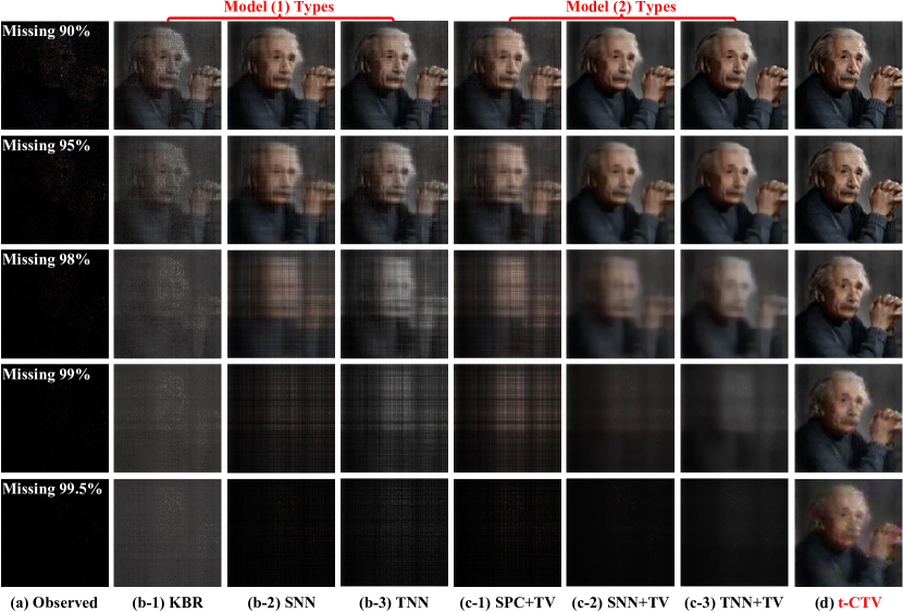
Figure 1: Illustration of recovery performance of all competing methods in color image inpainting. (a) Observed “Einstein” image with $90\%,95\%,98\%,99\%$ and $99.5\%$ missing pixels (from up to bottom); (b) Recovery obtained by several SOTA methods built under model (1): (b-1) KBR[30], (b-2) SNN[6], (b-3) TNN[29]; (c) Recovery obtained by several SOTA methods built under model (2): (c-1) SPC+TV[23], (c-2) SNN+TV[21], (c-3) TNN+TV[28]; (d) Recovery by our method. It can be seen that our method can still work while all its peers largely failed in the last extreme missing case.

2 Related Works

2.1 Low-rank tensor recovery

We take TC and TRPCA, two of the most commonly studied tensor recovery tasks, as examples to introduce the related L-prior works. Specifically, TC refers to the problem of recovering a low-rank tensor $\mathcal{T}_{0}$ from its partial entries, i.e.,

$$\min_{\mathcal{T}}\mathfrak{R}(\mathcal{T})\ \ \text{s.t.}\ \ \mathscr{P}_{\Omega}(\mathcal{T})=\mathscr{P}_{\Omega}(\mathcal{T}_{0}),$$ (3)

where $\Omega$ is the known elements’ index and $\mathscr{P}(\cdot)$ is the projection operator. TRPCA aims to achieve recovery from grossly corrupted observations, modeled as:

$$\min_{\mathcal{T,E}}\mathfrak{R}(\mathcal{T})+\lambda\|\mathcal{E}\|_{1}\ \ \text{s.t.}\ \ \mathcal{M}=\mathcal{T}+\mathcal{E},$$ (4)

where $\mathcal{E}$ represents the noise component characterized by the $L_{1}$-norm $\|\cdot\|_{1}$ and $\lambda>0$ denotes the trade-off parameter.

Low-rank tensor recovery is originally developed from low-rank matrix recovery [31, 32], but fraught with more challenges since the low-rank representation of a tensor is not unique. The early works are mainly established upon Tucker decomposition. Liu et al. [6] first proposed the sum of nuclear norm (SNN) and implemented it in TC tasks as an extension of matrix’s nuclear norm method to tensors, which greatly promotes the development of tensor recovery in visual data processing. Later on, Goldfarb and Qin [33] extended TRPCA problem in aspect of algorithm and Huang et al. [7] filled the gap in theory. Unfortunately, it’s proved that SNN is not the tightest convex relaxation [34], thus leading to suboptimality of the solution [35]. Several literatures attempted to ameliorate this issue. E.g., Mu et al. [35] proposed a better convexification based on a balanced matricization strategy and proved a lower bound in sampling complexity. Xie et al. [30] further transformed the Tucker decomposition as a representation form of Kronecker basis and proposed the KBR tensor sparsity, resulting significant improvements both in TC and TRPCA tasks. Some other works are proposed with nonconvex relaxation and matrix factorization (MF) on Tucker mode-wise matrices [36, 37]. Except for the Tucker decomposition based research, in [38], Zhao et al. proposed a fully Bayesian probabilistic CP factorization for TC problem, and several works further studied robust tensor CP decomposition problem [39, 40]. Besides, there also exist a series of works using certain type of tensor network decompositions [11, 12], see [41, 42, 43, 44].

Another class of works are based on t-SVD [13]. It provides a more appropriate extension of matrix SVD. Compared with Tucker decomposition, t-SVD does not need matricization, and more importantly, equips the optimality property in low-rank representation as well as the matrix SVD [14]. Formally, it decomposes a tensor into a tensor-tensor product of two orthogonal tensors and a f-diagonal tensor (also called as singular value tensor), and thus induces the t-SVD rank, also called tubal rank [45] for third-order tensors, defined as the number of nonzero tubes of the singular value tensor. Based on that, a heuristic tensor nuclear norm (TNN) as the convex surrogate of tubal rank is defined in [46], and then Zhang and Aeron [15] used it in TC tasks with theoretical guarantee. Then, a new form of TNN was proposed with the tightest convex envelope property and investigated in several tensor recovery problems [16, 47]. Recently, substantial investigations on t-SVD based tensor-related problems have been constructed, such as [48, 49, 50, 17, 51, 18]. Although these methods have attracted much attention, they cannot be applied to tensors of arbitrary order directly. Very recently, as an extension of the series of works by Kilmer et al. [13, 52, 53, 14], in [29], Qin et al. made a successful advancement with transform induced high-order t-SVD, exhibiting fine potentials in tensor recovery.

2.2 Joint low-rank and smooth tensor recovery

We then review related methods for jointly considering L and S priors for tensor recovery.

The S-prior structure is well possessed by a variety of visual tensor data, and generally modeled by total variation (TV). It can be simply divided into anisotropic TV (TV-1) and isotropic TV (TV-2) cases, defined by the absolute distance and square distance on the difference of the neighbor elements, respectively [54]. In practice, researchers always design certain variations of TV form corresponding to the type of data. For a simple image, one often use spatial TV (STV) to characterize the piecewise smooth structure along its spatial dimensions [55, 56, 57]. For hyperspectral images (HSIs), there also exists smoothness along its spectral direction, thus leading to the spectral-spatial TV (SSTV) [58, 59]. Similarly, the temporal-spatial TV is also formulated for videos [60]. For other TV variations, see [61, 62, 63].

Recently, the TV approaches have been widely adopted in the visual tensor data recovery tasks, most of which are used via a joint model with low-rank and TV regularizers. Typically, Ji et al. [20] investigated the TC problem by embedding the STV into the low-rank matrix factorization to all-mode matricization framework, While Li et al. [21] used the SNN to characterize the L prior, and the simple TV-1 on all-mode unfolding matrices for S prior. Other typical works along this line include [23, 22, 24, 25, 26, 27], partially summarized in Table I. These methods all employ a sum of L and S regularization terms, and have not proved exact-recovery results from a theoretical perspective. As a contrast, the basic tensor recovery models by purely using L regularizer can often establish the related theory guarantees, e.g., [7, 15, 16, 17, 19, 18, 51]. By the way, it should be noted that there are several theoretical works related to smooth data recovery, e.g., [64, 65, 66, 67], but the corresponding modeling and analyzing are only considered in vector or matrix space which cannot be directly used for joint low-rank and smooth tensor recovery.

TABLE I: Summary of some related works on tensor recovery with joint L+S priors

Literature	Problem	Model	Theory
Ji et al. [20]	TC	MF + STV	✘
Li et al. [21]	TC	SNN + TV-1	✘
Ko et al. [27]	TC	TT + TV-2	✘
Yokota et al. [23]	TC	CP + TV-1/TV-2	✘
He et al. [22]	TRPCA	MF + STV	✘
Wang et al. [24]	TRPCA	SNN + SSTV	✘
Chen et al. [25]	TRPCA	TNN + HTV	✘
Zhang et al. [26]	TRPCA	NLTRD + SSTV	✘
This work	TC$\&$TRPCA	t-CTV	✔

Against the aforementioned issues, this work proposes a unique tensor recovery regularizer encoding both L and S priors simultaneously. It adopts a type of fused prior modeling manner under the advanced high-order t-SVD algebraic framework, wherein the considered TC and TRPCA models both have exact recoverability guarantees in theory beyond current L+S tensor recovery models. The concise form of this specifically designed regularizer also naturally helps get rid of the difficulty of tuning the trade-off parameter imposed between two regularizers as conventional.

3 High-order t-SVD Framework

We first introduce high-order t-SVD framework briefly and provide its optimal representation theory in this section. Please refer to [13, 14, 52, 53, 29] for more details.

For an order-$d$ tensor $\mathcal{T}$ sized $n_{1}\times n_{2}\times\cdots\times n_{d}$, $\mathcal{T}(i_{1},i_{2},\cdots,i_{d})$ denotes its $(i_{1},i_{2},\cdots,i_{d})$-th element, and $\mathcal{T}(:,:,i_{3},\cdots,i_{d})$ is called as its $(i_{3},\cdots,i_{d})$-th face slice containing the first two modes which is also written as $\mathrm{T}^{(i_{3},\cdots,i_{d})}$. Then $\operatorname{bdiag}(\mathcal{T})$ sized $n_{1}\prod_{j=3}^{d}n_{j}\times n_{2}\prod_{j=3}^{d}n_{j}$ is the block diagonal matrix constructed by all face slices, which is also written as $\overline{\mathcal{T}}$.

For the t-SVD framework with invertible transform $\mathfrak{L}$ [29], a high-order tensor $\mathcal{T}$’s transform form is given by $\mathcal{T}_{\mathfrak{L}}:=\mathfrak{L}(\mathcal{T})=\mathcal{T}\times_{3}\mathrm{U}_{n_{3}}\times_{4}\cdots\times_{d}\mathrm{U}_{n_{d}}$, where $\times_{j}$ denotes mode-$j$ product ($\mathcal{Y}=\mathcal{X}\times_{j}\mathrm{M}$ means each $\mathcal{Y}(\cdots,i_{j-1},:,i_{j+1},\cdots)$ equals $\mathrm{M}\cdot\mathcal{X}(\cdots,i_{j-1},:,i_{j+1},\cdots)$ )and $\mathrm{U}_{n_{j}}$ is transform matrix sized $n_{j}\times n_{j}$, $j=3,\cdots,d$, such as the discrete fourier transform (DFT) and discrete cosine transform (DCT) matrices. Its inverse operation is $\mathfrak{L}^{-1}(\mathcal{T}):=\mathcal{T}\times_{3}\mathrm{U}_{n_{3}}^{-1}\times_{4}\cdots\times_{d}\mathrm{U}_{n_{d}}^{-1}$ and satisfies $\mathfrak{L}^{-1}(\mathfrak{L}(\mathcal{T}))=\mathcal{T}$. The transform matrices $\{\mathrm{U}_{n_{j}}\}_{j=3}^{d}$ of $\mathfrak{L}$ are assumed to satisfy

$$(\mathrm{U}_{n_{d}}^{*}\otimes\cdots\otimes\mathrm{U}_{n_{3}}^{*})\cdot(\mathrm{U}_{n_{d}}\otimes\cdots\otimes\mathrm{U}_{n_{3}})=\ell\cdot I_{n_{3}\cdots n_{d}},$$ (5)

where $(\cdot)^{*}$ is conjugate transpose, $\otimes$ denotes the Kronecker product, $I$ denotes unitary matrix and $\ell>0$ is a specific scale factor corresponding to the transform, e.g., $\ell=\prod_{j=3}^{d}n_{j}$ for DFT matrix $\mathrm{F}_{n_{j}}$ since $\mathrm{F}_{n_{j}}^{*}\mathrm{F}_{n_{j}}=n_{j}I_{n_{j}}$, and $\ell=1$ for DCT matrix $\mathrm{C}_{n_{j}}$ since $\mathrm{C}_{n_{j}}^{*}\mathrm{C}_{n_{j}}=I_{n_{j}}$, $j=3,\cdots,d$.

Definition 1 (tensor-tensor product[29]).

For order-$d$ tensors $\mathcal{A}\in\mathbb{R}^{n_{1}\times l\times n_{3}\times\cdots\times n_{d}}$ and $\mathcal{B}\in\mathbb{R}^{l\times n_{2}\times n_{3}\times\cdots\times n_{d}}$, its transform $\mathfrak{L}$ based product is defined as

$$\mathcal{A}*_{\mathfrak{L}}\mathcal{B}=\mathfrak{L}^{-1}(\mathfrak{L}(\mathcal{A})\Delta\mathfrak{L}(\mathcal{B})),$$ (6)

where $\Delta$ denotes the face-wise product ($\mathcal{Z}=\mathcal{X}\Delta\mathcal{Y}\Leftrightarrow\mathrm{Z}^{(i_{3},\cdots,i_{d})}=\mathrm{X}^{(i_{3},\cdots,i_{d})}\mathrm{Y}^{(i_{3},\cdots,i_{d})}$ for all face slices).

The tensor-tensor product leads that $\mathcal{C}=\mathcal{A}*_{\mathfrak{L}}\mathcal{B}$ is equivalent to $\overline{\mathcal{C}_{\mathfrak{L}}}=\overline{\mathcal{A}_{\mathfrak{L}}}\cdot\overline{\mathcal{B}_{\mathfrak{L}}}$. This conducts a simple implement of (6) by $\prod_{j=3}^{d}{n_{j}}$ times pairwise matrix product in the transform domain and then run inverse transformation.

Definition 2 (transpose [29]).

For $\mathcal{T}\in\mathbb{R}^{n_{1}\times n_{2}\times n_{3}\times\cdots\times n_{d}}$, its transpose $\mathcal{T}^{\mathrm{T}}\in\mathbb{R}^{n_{2}\times n_{1}\times n_{3}\times\cdots\times n_{d}}$ satisfies that $\mathcal{T}^{\mathrm{T}}_{\mathfrak{L}}(:,:,i_{3},\cdots,i_{d})=\mathcal{T}_{\mathfrak{L}}(:,:,i_{3},\cdots,i_{d})^{\mathrm{T}}$ for all face slices.

Definition 3 (identity tensor[29]).

An order-$d$ tensor $\mathcal{I}_{n}\in\mathbb{R}^{n\times n\times n_{3}\times\cdots\times n_{d}}$ is called as identity tensor if it satisfies $\mathcal{I}_{\mathfrak{L}}(:,:,i_{3},\cdots,i_{d})=I_{n}$ for all face slices.

Definition 4 (orthogonal tensor[29]).

An order-$d$ tensor $\mathcal{U}\in\mathbb{R}^{n\times n\times n_{3}\times\cdots\times n_{d}}$ is orthogonal if $\mathcal{U}^{\mathrm{T}}*_{\mathfrak{L}}\mathcal{U}=\mathcal{U}*_{\mathfrak{L}}\mathcal{U}^{\mathrm{T}}=\mathcal{I}_{n}$.

Definition 5 (f-diagonal tensor[29]).

An order-$d$ tensor $\mathcal{T}\in\mathbb{R}^{n\times n\times n_{3}\times\cdots\times n_{d}}$ is f-diagonal if all its face slices is diagonal.

Theorem 1 (t-SVD[29]).

For any order-$d$ tensor $\mathcal{T}\in\mathbb{R}^{n_{1}\times n_{2}\times\cdots\times n_{d}}$, it can be decomposed as

$$\mathcal{T}=\mathcal{U}*_{\mathfrak{L}}\mathcal{S}*_{\mathfrak{L}}\mathcal{V}^{\mathrm{T}},$$ (7)

where $\mathcal{U}\in\mathbb{R}^{n_{1}\times n_{1}\times\cdots\times n_{d}}$ and $\mathcal{V}\in\mathbb{R}^{n_{2}\times n_{2}\times\cdots\times n_{d}}$ are orthogonal, and $\mathcal{S}\in\mathbb{R}^{n_{1}\times n_{2}\times\cdots\times n_{d}}$ is a f-diagonal tensor.

Similar to the normal t-SVD with DFT transform [13, 52], the above general invertible linear transforms induced t-SVD can be realized by performing SVD on each slice of $\mathcal{T}_{\mathfrak{L}}$ in the transform domain and then inverting the corresponding components back to the original domain. Besides, the t-SVD has a skinny form [29] with the following t-SVD rank, and some concepts can be further established.

Definition 6 (t-SVD rank [29]).

For $\mathcal{T}\in\mathbb{R}^{n_{1}\times n_{2}\times\cdots\times n_{d}}$ with t-SVD $\mathcal{T}=\mathcal{U}*_{\mathfrak{L}}\mathcal{S}*_{\mathfrak{L}}\mathcal{V}^{\mathrm{T}}$, its t-SVD rank is defined as

$$\operatorname{rank}_{\operatorname{t-SVD}}(\mathcal{T}):=\sharp\{i:\mathcal{S}(i,i,:,\cdots,:)\neq\textbf{0}\},$$ (8)

where $\sharp$ denotes the cardinality of a set.

Definition 7 (tensor nuclear norm[29]).

For order-$d$ tensor $\mathcal{T}\in\mathbb{R}^{n_{1}\times n_{2}\times\cdots\times n_{d}}$ under the t-SVD framework with transform $\mathfrak{L}$, its tensor nuclear norm (TNN) is defined as

$$\|\mathcal{T}\|_{\circledast,\mathfrak{L}}:=\frac{1}{\ell}\sum_{i_{3}=1}^{n_{3}}\cdots\sum_{i_{d}=1}^{n_{d}}\|\mathcal{T}_{\mathfrak{L}}(:,:,i_{3},\cdots,i_{d})\|_{*},$$ (9)

where $\|\cdot\|_{*}$ denotes the nuclear norm of a matrix.

Theorem 2 (order-$d$ t-SVT[29]).

Given $\mathcal{T}\in\mathbb{R}^{n_{1}\times n_{2}\times\cdots\times n_{d}}$ with t-SVD $\mathcal{T}=\mathcal{U}*_{\mathfrak{L}}\mathcal{S}*_{\mathfrak{L}}\mathcal{V}^{\mathrm{T}}$, its tensor singular value thresholding (t-SVT) is defined by $\operatorname{t-SVT}_{\tau}(\mathcal{T}):=\mathcal{U}*_{\mathfrak{L}}\mathcal{S}_{\tau}*_{\mathfrak{L}}\mathcal{V}^{\mathrm{T}}$, where $\mathcal{S}_{\tau}=\mathfrak{L}^{-1}((\mathcal{S}_{\mathfrak{L}}-\tau)_{+})$, $t_{+}=\max(0,t)$, which obeys

$$\operatorname{t-SVT}_{\tau}(\mathcal{T})=\arg\min_{\mathcal{X}}\tau\|\mathcal{X}\|_{\circledast,\mathfrak{L}}+\frac{1}{2}\|\mathcal{X}-\mathcal{T}\|_{\mathrm{F}}^{2}.$$ (10)

Very recently, Kilmer et al. [14] proved that tensor format equips the optimality over its flattening matrix in low-rank approximation via the normal order-3 t-SVD. Here, we present a generic result, which reveals the necessity and natural advantage of the direct study on high-order tensors.

Theorem 3 (optimality principle).

Given the t-SVD of $\mathcal{T}\in\mathbb{R}^{n_{1}\times n_{2}\times\cdots\times n_{d}}$ by $\mathcal{T}=\mathcal{U}*_{\mathfrak{L}}\mathcal{S}*_{\mathfrak{L}}\mathcal{V}^{\mathrm{T}}$, then, $\mathcal{T}_{k}:=\sum_{i=1}^{k}\mathcal{U}(:,i,:,\cdots,:)*_{\mathfrak{L}}\mathcal{S}(i,i,:,\cdots,:)*_{\mathfrak{L}}\mathcal{V}(:,i,:,\cdots,:)^{\mathrm{T}}$ is the best Frobenius norm approximation over all t-SVD rank-$k$ tensor. Moreover, suppose $\mathrm{M}$ is any unfolding matrix of $\mathcal{T}$, we have,

$$\operatorname{rank}_{\operatorname{t-SVD}}(\mathcal{T})\leq\operatorname{rank}(\mathrm{M}),$$ (11)

and

$$\|\mathcal{T}-\mathcal{T}_{k}\|_{\mathrm{F}}\leq\|\mathrm{M}-\mathrm{M}_{k}\|_{\mathrm{F}},$$ (12)

where $\mathrm{M}_{k}$ is the rank-$k$ approximation of the matrix $\mathrm{M}$.

4 Tensor Correlated Total Variation

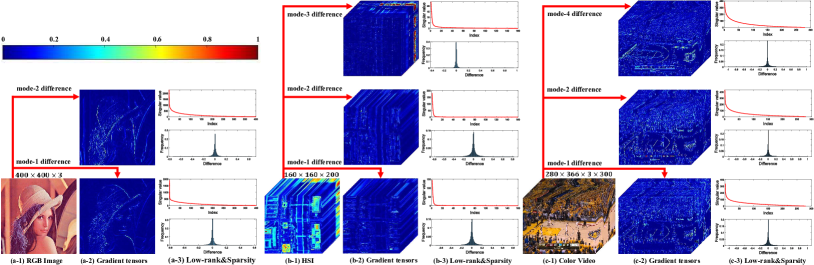
Figure 2: Illustrations of simultaneous L and S prior structures in correlated gradient tensors. (a-1), (b-1), (c-1): three typical types of visual tensor data: RGB image, HSI and color video; (a-2), (b-2), (c-2): their correlated gradient tensors; (a-3), (b-3), (c-3): the corresponding curves of tensor singular values (upper) and frequency histograms of all their elements (below).

Considering a tensor $\mathcal{T}\in\mathbb{R}^{n_{1}\times\cdots\times n_{d}}$ with joint L and S priors, its low-rank property can be well characterized via the rank surrogates under the aforementioned high-order t-SVD decomposition, like the TNN. Its smoothness, on the other hand, is often captured by the low energy of $\mathcal{T}$’s gradient tensors using certain TV (semi)-norm. We first formally define such gradient tensor as follows:

Definition 8 (gradient tensor).

For $\mathcal{T}\in\mathbb{R}^{n_{1}\times\cdots\times n_{d}}$, its gradient tensor along the $k$-th mode is defined by

$$\mathcal{G}_{k}:=\nabla_{k}(\mathcal{T})=\mathcal{T}\times_{k}\mathrm{D}_{n_{k}},\ k=1,2,\cdots,d,$$ (13)

where $\mathrm{D}_{n_{k}}$ is a row circulant matrix of $(-1,1,0,\cdots,0)$.

The anisotropic TV (TV-1) and the isotropic TV (TV-2) are defined as $\|\mathcal{T}\|_{\operatorname{TV-1}}:=\sum_{k\in\Gamma}\|\mathcal{G}_{k}\|_{1}$ and $\|\mathcal{T}\|_{\operatorname{TV-2}}:=\sum_{k\in\Gamma}\|\mathcal{G}_{k}\|_{\mathrm{F}},$ respectively, where $\Gamma$ is a priori set consisting of certain directions that $\mathcal{T}$ equips smooth continuity along these modes. For instances, images are often assumed with local smoothness along the spatial directions, i.e., $\Gamma=\{1,2\}$. HSIs and color videos have further spectral and temporal smoothness respectively, except spatial smoothness, thus $\Gamma$ can be set as $\{1,2,3\}$ and $\{1,2,4\}$ respectively. For easy notation, the two forms of TV norm are all denoted as $\|\mathcal{T}\|_{\operatorname{TV}}$ throughout the paper.

Considering a structured tensor with simultaneous L and S priors, it is natural for existing research to generally use a sum of two separate regularizers for encoding such two priors, easily following the L+S models. Different from the previous methods, our aim is to represent both L+S priors on the gradient tensors, and especially specify a unique regularization term for concisely delivering both prior information simultaneously. This also finely complies with the fact that the two priors are always coexist with each other in natural visual tensor data, but not independently occur as the conventional models with separate L and S regularizers implicitly imply. This can be evidently observed from Fig. 2, which illustrates such phenomenon visually on several typical types of visual tensor data. We name this proposed regularizer as tensor correlated total variation (t-CTV), defined in the following:

Definition 9 (t-CTV).

For $\mathcal{T}\in\mathbb{R}^{n_{1}\times\cdots\times n_{d}}$, denote $\Gamma$ as a priori set consisting of directions along which $\mathcal{T}$ equips L+ S priors, and $\mathcal{G}_{k},k\in\Gamma$ as its correlated gradient tensors. We define a tensor correlated total variation (t-CTV) norm as

$$\|\mathcal{T}\|_{\operatorname{t-CTV}}:=\frac{1}{\gamma}\sum_{k\in\Gamma}\|\mathcal{G}_{k}\|_{\circledast,\mathfrak{L}},$$ (14)

where $\gamma:=\sharp\{\Gamma\}$ equals the cardinality of $\Gamma$.

(a) TNN	(b) TV-1	(c) TV-2	(d) t-CTV

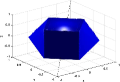
(a)

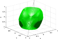
(b)

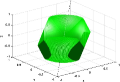
(c)

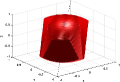
(d)

Figure 3: Manifolds of the TNN, TV and t-CTV norm.

From the perspective of L-prior encoding, the t-CTV constrains the TNN metric of correlated gradient tensors $\mathcal{G}_{k}$ intuitively, which naturally promotes $\mathcal{G}_{k}$’s low-rankness property, and then enhances the similar prior structure of the original tensor, as validated in the following remark:

Remark 1.

For $\mathcal{T}\in\mathbb{R}^{n_{1}\times\cdots\times n_{d}}$ with t-SVD rank $R$, it can be verified that $R-1\leq\operatorname{rank}_{\operatorname{t-SVD}}(\mathcal{G}_{k})\leq R,$ where $\mathcal{G}_{k}$ is the gradient tensor along $k$-th mode. This means that the low-rankness between the original and gradient tensors are consistent, indicating that the t-CTV can indirectly induce the expected L-prior structure of the original tensor like a low-rank regularizer.

Besides, from the perspective of S-prior encoding, since the t-CTV is a norm defined in the gradient domain, it measures as an energy control term that tends the discrete first-order derivatives of the tensor data along certain smoothness prior modes being small numerical values. This is similar to the TV norm.

Remark 2.

For $\mathcal{T}\in\mathbb{R}^{n_{1}\times\cdots\times n_{d}}$ with t-SVD rank $R$, it can be verified that $\|\mathcal{T}\|_{\operatorname{TV}}\lesssim\|\mathcal{T}\|_{\operatorname{t-CTV}}\lesssim\sqrt{R}\|\mathcal{T}\|_{\operatorname{TV}}$, meaning that the t-CTV and TV are compatible in sense of norm. From the viewpoint of energy minimization, both t-CTV and TV norm tend to be smaller when $\mathcal{T}$ becomes smoother, and take the minimum value of zero only if $\mathcal{T}$ is absolutely flat, indicating that the t-CTV can also indirectly induce the expected S-prior structure of the targeted tensor like a TV regularizer.

Combining the above two points, it is expected that the t-CTV can finely encode both the L and S priors. To more intuitively observe its capability on constraining the two priors, we plot the manifolds of TNN, TV and t-CTV norm in Fig. 3. One can see that the manifold of t-CTV has evident similarity to that of TV norm in the whole shape, and also exists some close characteristics with TNN like the two tangent planes seen from the front, showing the close connections in constraining the solution space in terms of low-rankness and smoothness, respectively.

Besides, it should be noted that although the t-CTV is not the unique encoding term for L nor S prior, it still achieves much better performance for joint low-rank and smooth tensor recovery than existing pure L, S and L+S models, which will be demonstrated in the following experiments.

5 Tensor Recovery via t-CTV Minimization

5.1 Models

Suppose $\mathcal{T}_{0}\in\mathbb{R}^{n_{1}\times\cdots\times n_{d}}$ is the underlying unknown tensor with joint L and S structural assumption. For the TC problem, we adopt the commonly used random Bernoulli sampling scheme, $\Omega\sim\operatorname{Ber}(p)$. Using t-CTV to characterize the L and S priors, the conducted t-CTV based TC model is

$$\min_{\mathcal{T}}\|\mathcal{T}\|_{\operatorname{t-CTV}}\ \ \text{s.t.}\ \ \mathscr{P}_{\Omega}(\mathcal{T})=\mathscr{P}_{\Omega}(\mathcal{T}_{0}).$$ (15)

For the TRPCA problem, the observation of $\mathcal{T}_{0}$ is a corruption with outlier or noise $\mathcal{E}_{0}$, denoted as $\mathcal{M}=\mathcal{T}_{0}+\mathcal{E}_{0}.$ Then the t-CTV based TRPCA problem is modeled as

$$\min_{\mathcal{T},\mathcal{E}}\|\mathcal{T}\|_{\operatorname{t-CTV}}+\lambda\|\mathcal{E}\|_{1}\ \ \text{s.t.}\ \ \mathcal{M}=\mathcal{T}+\mathcal{E}.$$ (16)

The following recovery guarantees aim to ensure that $\mathcal{T}_{0}$, $(\mathcal{T}_{0},\mathcal{E}_{0})$ are the exact solutions of (15) and (16), respectively, with some mild conditions.

5.2 Incoherence Conditions

Note that t-CTV is actually constructed by the tensor nuclear norm imposed on related gradient tensors under the high order t-SVD framework. Thus the theoretical analytical framework of classic low-rank tensor recovery can be readily borrowed. The incoherence condition is one of the most vital theoretical tools in low-rank recovery [15][29][31][69]. Below, we define the gradient tensor incoherence conditions, whose purpose is the same with that in the classic low-rank analysis. That is to impose or constraint the low-rankness structure of the underlying tensor, avoiding the pathological issue or hopeless case, i.e., most elements of $T_{0}$ are zero but it is low-rank. More descriptions are in [15][29][31][69].

Definition 10.

For $\mathcal{T}\in\mathbb{R}^{n_{1}\times\cdots\times n_{d}}$ with t-SVD rank $R$, and any $k\in\Gamma$, assume that the gradient tensors $\mathcal{G}_{i}$s have the skinny t-SVD $\mathcal{G}_{k}=\mathcal{U}_{k}*_{\mathfrak{L}}\mathcal{S}_{k}*_{\mathfrak{L}}\mathcal{V}_{k}^{\mathrm{T}}$, and then $\mathcal{T}$ is said to satisfy the gradient tensor incoherence conditions with parameter $\mu>0$ if

$$\max_{i_{1}=1,\cdots,n_{1}}\|\mathcal{U}_{k}^{\mathrm{T}}*_{\mathfrak{L}}\mathring{\mathfrak{e}}_{1}^{(i_{1})}\|_{\mathrm{F}}^{2}\leq{\mu R}/{n_{1}\ell},$$ (17)

$$\max_{i_{2}=1,\cdots,n_{2}}\|\mathcal{V}_{k}^{\mathrm{T}}*_{\mathfrak{L}}\mathring{\mathfrak{e}}_{2}^{(i_{2})}\|_{\mathrm{F}}^{2}\leq{\mu R}/{n_{2}\ell},$$ (18)

and

$$\|\mathcal{U}_{k}*_{\mathfrak{L}}\mathcal{V}_{k}^{\mathrm{T}}\|_{\infty}^{2}\leq{\mu R}/{n_{1}n_{2}\ell^{2}},$$ (19)

where $\mathring{\mathfrak{e}}_{1}^{(i_{1})}$ is the order-$d$ tensor mode-1 basis sized $n_{1}\times 1\times n_{3}\times\cdots\times n_{d}$, whose $(i_{1},1,1,\cdots,1)$-th entry equals 1 and the rest equal 0, and $\mathring{\mathfrak{e}}_{2}^{(i_{2})}:=(\mathring{\mathfrak{e}}_{1}^{(i_{2})})^{\mathrm{T}}$ is the mode-2 basis.

The difference between the above incoherence conditions and previous ones is that it is imposed on the gradient tensors instead of the original tensor. Note that [69] has proved that almost all uniformly bounded low-rank matrices equip incoherence property well. Since difference operation on a tensor changes neither its boundness nor low-rankness, the incoherence conditions naturally hold on its gradient maps. The first two conditions (17), (18) and the third one (19) are normally called the standard and joint incoherence conditions, associated with TC and TRPCA problem, respectively.

5.3 Main Results

We firstly show the exact recovery guarantee of the proposed t-CTV-TC model (15).

Theorem 4.

Consider t-CTV based TC model (15). Suppose that $\mathcal{T}_{0}$ obeys the standard gradient tensor incoherence conditions (17)-(18) and $\Omega\sim\operatorname{Ber}(p)$. Then, there exist universal constants $c_{0},c_{1},c_{2}>0$ such that $\mathcal{T}_{0}$ is the unique solution to model (15) with probability at least $1-c_{1}\gamma(n_{(1)}n_{3}\cdots n_{d})^{-c_{2}}$, provided that

$$p\geq c_{0}\mu R(\log(n_{(1)}\ell))^{2}/n_{(2)}\ell,$$ (20)

where $\ell$ is the specific scale factor given in (5), $n_{(1)}:=\max\{n_{1},n_{2}\}$ and $n_{(2)}:=\min\{n_{1},n_{2}\}$.

The above result shows that minimizing t-CTV norm can achieve exact tensor completion with considerable probability. The corresponding sampling complexity needs to be around $p\cdot\prod_{i=1}^{d}n_{i}\approx O(\mu Rn_{(1)}n_{3}\cdots n_{d}\log^{2}(n_{(1)}\ell)/\ell)$. Such a bound can be acceptable if considering only the low-rankness since it differs from the degrees of freedom of an arbitrary order-$d$ tensor with t-SVD rank $R$, i.e., $O(Rn_{(1)}n_{3}\cdots n_{d})$, by a logarithmic factor. But, for a joint L and S prior structured tensor, its degree of freedom should be lower than that of a pure low-rank tensor with the same rank, which indicates that its sampling complexity for recovery could be further improved. Below, we introduce an important proposition on the lower bound for general regularization norm based TC model inspired from [70].

Proposition 1.

Let $\mathcal{T}_{0}\in\mathbb{R}^{n_{1}\times\cdots\times n_{d}}$ with multi-structural prior simultaneously. Consider the following general TC model

$$\min_{\mathcal{T}}f(\mathcal{T}):=\sum w_{i}\|\mathcal{T}\|_{(i)}\ \ \text{s.t.}\ \ \mathscr{P}_{\Omega}(\mathcal{T})=\mathscr{P}_{\Omega}(\mathcal{T}_{0}),$$ (21)

where $\|\cdot\|_{(i)}$ denotes a regularization norm (such as TNN, TV, and t-CTV norm) modeling certain prior with Lipschitz constant $L_{i}$, $w_{i}>0$ is the wight parameter. Suppose $\Omega\sim\operatorname{Ber}(p)$ and $m$ is the number of sampling entries. Then, there exist constant $c_{0},c_{1}>0$ such that $\mathcal{T}_{0}$ is not the unique solution of (21) with probability at least $1-\exp(-\frac{c_{1}m}{n_{1}\cdots n_{d}\|\bar{\mathcal{T}}_{0}\|_{\infty}^{2}})$, provided that

$$m\leq m_{\operatorname{low}}:=c_{0}\kappa_{\operatorname{min}}^{2}n_{1}\cdots n_{d},$$ (22)

where $\kappa_{\operatorname{min}}=\min\{\kappa_{i}=\|\bar{\mathcal{T}_{0}}\|_{(i)}/L_{i}\}$ and $\bar{\mathcal{T}}_{0}=\mathcal{T}_{0}/\|\mathcal{T}_{0}\|_{\mathrm{F}}$.

Proposition 1 states an interesting and enlightening result that the linear combination of multi-structures promoted regularization norm can do no better than using only the best single one. It can be only determined by one single regularizer for multi-structural tensor completion in terms of the boundary of failure recovery. That provides a strong evidence that to fully explore the multiple priors, we might necessarily need to design certain new regularizer to character the joint structures, as also claimed in [71, 70, 35]. This actually motivates us for designing the t-CTV term to reprace previous L+S terms with summarization of two elements. Now, we show that the t-CTV model (15) owns an interpretable lower sampling bound and is superior over those of pure L, S and joint L+S prior models.

Theorem 5.

For order-$d$ tensor $\mathcal{T}_{0}\in\mathbb{R}^{N\times\cdots\times N}$ with L and S prior structures simultaneously, denote its t-SVD rank as $R$ and gradient tensor $\mathcal{G}_{k}$’s sparsity (number of nonzero entries) as $S_{k}$, and $S=\min_{k\in\Gamma}\{S_{k}\}$. Then, the corresponding lower bounds of the following L and/or S models satisfy:

Model	$f(\mathcal{T})=$	$m_{\operatorname{low}}\lesssim$
L	$\|\mathcal{T}\|_{\circledast,\mathfrak{L}}$	$N^{d}\cdot\frac{R}{N}$
S	$\|\mathcal{T}\|_{\operatorname{TV}}$	$N^{d}\cdot\frac{S}{N^{d}}$
L+S	$\|\mathcal{T}\|_{\circledast,\mathfrak{L}}+\alpha\|\mathcal{T}\|_{\operatorname{TV}}$	$N^{d}\cdot\min\{\frac{R}{N},\frac{S}{N^{d}}\}$
t-CTV	$\|\mathcal{T}\|_{\operatorname{t-CTV}}$	$N^{d}\cdot\frac{R}{N}\cdot\frac{S}{N^{d}}$

As presented in Theorem 5, t-CTV’s lower bound, i.e.,

$$N^{d}\cdot\frac{R}{N}\cdot\frac{S}{N^{d}},$$ (23)

is a product interaction form of the L and S metrics in an interpretable manner, that is rigorously less than that of the pure L and S regularization models and the widely adopted L+S ones if the underlying tensor is low-rank and smooth simultaneously. This certainly explains why our method achieves nice performance in even extremely small sampling rate, as shown in Fig. 1. The lower the rank ratio $R/N$ is, and the lower the smooth ratio $S/N^{d}$ is, the lower the informatic bound of our t-CTV model should be. Whereas, existing L+S modeling manner cannot so intrinsically fuse the two priors from this theoretical perspective.

We then analyze of the t-CTV based TRPCA problem (16), whose recoverability can be also guaranteed.

Theorem 6.

Consider t-CTV based TRPCA model (16). Suppose that $\mathcal{T}_{0}$ obeys the standard and joint gradient tensor incoherence conditions (17)-(19) and $\mathcal{E}_{0}$’s support set, denoted as $\Omega_{0}$, is uniformly distributed among all sets of cardinality $m$. Then, there exist universal constants $c_{1},c_{2}>0$ such that $(\mathcal{T}_{0},\mathcal{E}_{0})$ is the unique solution to model (16) when $\lambda=1/\sqrt{n_{(1)}\ell}$ with probability at least $1-c_{1}\gamma(n_{(1)}n_{3}\cdots n_{d})^{-c_{2}}$, provided that

$$\operatorname{rank}_{\operatorname{t-SVD}}(\mathcal{T}_{0})\leq\frac{\rho_{r}n_{(2)}\ell}{\mu\log^{2}(n_{(1)}\ell)}\ \ \text{and}\ \ m\leq\rho_{s}n_{1}\cdots n_{d},$$ (24)

where $\rho_{r},\rho_{s}>0$ are some numerical constants.

Theorem 6 states that the t-CTV induced TRPCA model (16) is able to exactly recover a joint L and S structured tensor and a sparse noise with high probability. The corresponding parameters $\rho_{r}$ and $\rho_{s}$ determine the rank of $\mathcal{T}_{0}$ and the sparsity of $\mathcal{E}_{0}$, respectively. Moreover, the analysis identifies that the model (16) is parameter-free where the trade-off parameter $\lambda=1/\sqrt{n_{(1)}\ell}$ is universal, making it easier to implement in applications.

Remark 3.

The above theoretical analysis provides solid support of the recoverability of t-CTV modeling in tensor recovery. The proof is mainly executed by possibly finely embedding the t-CTV model into the classic sparse modeling framework. Yet it should be indicated that such proof is not that easy since the dependent high-order t-SVD framework differs from common matrix algebra in many aspects. E.g., the linear conversion via tensor-tensor product is totally different from that in matrix space, and there exist difference operation and the low-rankness of gradient tensors required to be proved (see Appendix A, B and C). More importantly, the key dual certification process is different from previous works, where one needs to consider the difference transformation (see Lemmas 5 and 13 in Appendixes D and F, respectively).

Algorithm 1 ADMM for solving t-CTV-TC model (15)

0:  observation $\mathscr{P}_{\Omega}(\mathcal{T}_{0})$, priori set $\Gamma$ and transform $\mathfrak{L}$.

1:  Initialize $\mathcal{G}_{k}^{0}=\nabla_{k}(\mathscr{P}_{\Omega}(\mathcal{T}_{0}))$, $\mathcal{E}^{0}=\Upsilon^{0}=\Lambda_{k}^{0}=\mathcal{O}$.

2:  while not converge do

3:   Update $\mathcal{T}^{t+1}$ by (29);

4:   Update $\mathcal{G}_{k}^{t+1}$ by (30) for each $k\in\Gamma$;

5:   Update $\mathcal{K}^{t+1}$ by (31);

6:   Update multipliers $\Lambda_{k}^{t+1},k\in\Gamma$ and $\Upsilon^{t+1}$ by (32);

7:   Let $\mu_{t+1}=\rho\mu_{t}$; $t=t+1$.

8:  end while

8:  recovered tensor $\hat{\mathcal{T}}=\mathcal{T}^{t+1}$.

6 Optimization Algorithms

This section derives algorithms for solving the t-CTV based TC and TRPCA problem via the Alternating Direction Method of Multipliers (ADMM) framework [72].

6.1 Optimization to t-CTV TC

First, the t-CTV-TC model (15) can be reformulated as

$$\begin{split}&\min_{\mathcal{T},\mathcal{G}_{k},\mathcal{K}}\ \ \frac{1}{\gamma}\sum_{k\in\Gamma}\|\mathcal{G}_{k}\|_{\circledast,\mathfrak{L}}+\delta_{\mathcal{K},\Omega}\\ &\text{s.t.}\ \ \mathcal{G}_{k}=\nabla_{k}(\mathcal{T}),\mathcal{T}+\mathcal{K}=\mathscr{P}_{\Omega}(\mathcal{T}_{0}),\end{split}$$ (25)

where the auxiliary variable $\mathcal{G}_{k}$ separates the difference operation $\nabla_{k}(\cdot)$ and $\mathcal{K}$ compensates missing entries of $\mathcal{T}$ that is restricted in $\Omega^{\bot}$ using the indicative function defined as

$$\begin{split}\delta_{\mathcal{K},\Omega}=\left\{\begin{array}[]{ll}0,&\mathscr{P}_{\Omega}(\mathcal{K})=\mathcal{O},\\ +\infty,&\text{otherwise}.\end{array}\right.\end{split}$$ (26)

Then the augmented Lagrangian function of (25) is

$$\begin{split}&\ \ \ \ \mathcal{L}(\mathcal{T},\{\mathcal{G}_{k},k\in\Gamma\},\mathcal{K},\{\Lambda_{k},k\in\Gamma\},\Upsilon)=\\ &\sum_{k\in\Gamma}(\frac{1}{\gamma}\|\mathcal{G}_{k}\|_{\circledast,\mathfrak{L}}+\langle\Lambda_{k},\nabla_{k}(\mathcal{T})-\mathcal{G}_{k}\rangle+\frac{\mu_{t}}{2}\|\nabla_{k}(\mathcal{T})-\mathcal{G}_{k}\|_{\mathrm{F}}^{2})\\ &+\delta_{\mathcal{K},\Omega}+\langle\Upsilon,\mathscr{P}_{\Omega}(\mathcal{T}_{0})-\mathcal{T}-\mathcal{K}\rangle+\frac{\mu_{t}}{2}\|\mathscr{P}_{\Omega}(\mathcal{T}_{0})-\mathcal{T}-\mathcal{E}\|_{\mathrm{F}}^{2},\end{split}$$

where $\mu_{t}$ is a positive scalar, and $\Lambda_{k}$ and $\Upsilon$ are Lagrange multipliers. It can be further expressed as

$$\begin{split}&\ \ \mathcal{L}=\sum_{k\in\Gamma}(\frac{1}{\gamma}\|\mathcal{G}_{k}\|_{\circledast,\mathfrak{L}}+\frac{\mu_{t}}{2}\|\nabla_{k}(\mathcal{T})-\mathcal{G}_{k}+{\Lambda_{k}}/{\mu_{t}}\|_{\mathrm{F}}^{2})\\ &\ \ \ \ \ \ \ +\delta_{\mathcal{K},\Omega}+\frac{\mu_{t}}{2}\|\mathscr{P}_{\Omega}(\mathcal{T}_{0})-\mathcal{T}-\mathcal{K}+{\Upsilon}/{\mu_{t}}\|_{\mathrm{F}}^{2}+C,\end{split}$$ (27)

where $C$ is only the multipliers dependent squared items. Below, we show how to solve its sub-problems for each involved variable.

1) Updating $\mathcal{T}^{t+1}$: Taking the derivative in (27) with respect to $\mathcal{T}$, it gets the following linear system

$$\begin{split}&\ \ \ \ (\mathcal{I}+\sum\nabla_{k}^{\mathrm{T}}\nabla_{k})(\mathcal{T})\\ &=\mathscr{P}_{\Omega}(\mathcal{T}_{0})-\mathcal{K}^{t}+\Upsilon^{t}/\mu_{t}+\sum\nabla_{k}^{\mathrm{T}}(\mathcal{G}_{k}^{t}-\Lambda_{k}^{t}/\mu_{t}),\end{split}$$ (28)

where $\nabla_{k}^{\mathrm{T}}(\cdot)$ denotes the transpose operator of $\nabla_{k}(\cdot)$. Note that the difference operation on tensors has been proved to be linear via tensor-tensor product (see Appendix C, D). Following [57], we can apply multi-dimensional FFT, which diagonalizes $\nabla_{k}(\cdot)$’s corresponding difference tensors $\mathcal{D}_{k}$, enabling to efficiently get the optimal solution of (28) based on the convolution theorem of Fourier transforms, i.e.,

$$\mathcal{T}^{t+1}=\mathcal{F}^{-1}\left(\frac{\mathcal{F}(\mathscr{P}_{\Omega}(\mathcal{T}_{0})-\mathcal{K}^{t}+\Upsilon^{t}/\mu_{t})+\mathcal{H}}{\mathbf{1}+\sum_{k\in\Gamma}\mathcal{F}(\mathcal{D}_{k})^{*}\odot\mathcal{F}(\mathcal{D}_{k})}\right),$$ (29)

where $\mathcal{H}=\sum_{k\in\Gamma}\mathcal{F}(\mathcal{D}_{k})^{*}\odot\mathcal{F}(\mathcal{G}_{k}^{t}-\Lambda_{k}^{t}/\mu_{t}),$ $\mathbf{1}$ is a tensor with all entries as 1, $\odot$ is componentwise multiplication, and the division is componentwise as well.

2) Updating $\mathcal{G}_{k}^{t+1},k\in\Gamma$: For each $k\in\Gamma$, extracting all items containing $\mathcal{G}_{k}$ from (27), we can get that

$$\begin{split}\mathcal{G}_{k}^{t+1}=\arg\min_{\mathcal{G}_{k}}\frac{1}{\gamma}\|\mathcal{G}_{n}\|_{\circledast,\mathfrak{L}}+\frac{\mu_{t}}{2}\|\nabla_{k}(\mathcal{T}^{t+1})-\mathcal{G}_{k}+\frac{\Lambda_{k}^{t}}{\mu_{t}}\|_{F}^{2}.\end{split}$$

The close-form solution of this sub-problem is given as

$$\mathcal{G}_{k}^{t+1}=\operatorname{t-SVT}_{1/\gamma\mu_{t}}(\nabla_{k}(\mathcal{T}^{t+1})+{\Lambda_{k}^{t}}/{\mu_{t}})$$ (30)

via the order-$d$ t-SVT as stated in Theorem 2.

3) Updating $\mathcal{K}^{t+1}$: The optimization of $\mathcal{K}$ is based on that it obeys $\mathscr{P}_{\Omega}(\mathcal{K})=\mathcal{O}$. Thus, it is updated by performing

$$\mathcal{K}^{t+1}=\mathscr{P}_{\Omega}(\mathcal{T}_{0})-\mathcal{T}^{t+1}+{\Upsilon^{t}}/{\mu_{t}},\ \mathscr{P}_{\Omega}(\mathcal{K}^{t+1})=\mathcal{O}.$$ (31)

4) Updating $\Lambda_{k}^{t+1}$ and $\Upsilon^{t+1}$: Based on the ADMM’s rule, these multipliers are updated by the following equations:

$$\begin{split}\left\{\begin{array}[]{ll}\Lambda_{k}^{t+1}=\Lambda_{k}^{t}+\mu_{t}(\nabla_{k}(\mathcal{T}^{t+1})-\mathcal{G}_{k}^{t+1}),\ \forall k\in\Gamma,\\ \Upsilon^{t+1}=\Upsilon^{t}+\mu_{t}(\mathscr{P}_{\Omega}(\mathcal{T}_{0})-\mathcal{T}^{t+1}-\mathcal{K}^{t+1}).\end{array}\right.\end{split}$$ (32)

Last, the penalty parameter $\mu_{t+1}$ is lifted by $\mu_{t+1}=\rho\mu_{t}$ with some control constant $\rho>1$. The whole ADMM optimization scheme is summarized in Algorithm 1.

6.2 Optimization to t-CTV TRPCA

The optimization to t-CTV-TRPCA is quite similar to that to the t-CTV-TC problem. Its model reformulation and augmented Lagrangian function are similar like (25) and (27), except that auxiliary variable $\mathcal{K}$ are replaced by the sparse component $\mathcal{E}$ in model (16) with corresponding regularization $\lambda\|\mathcal{E}\|_{1}$, and the observation is $\mathcal{M}$ instead of $\mathscr{P}_{\Omega}(\mathcal{T}_{0})$. Thus, under similar analysis, the ADMM iteration system with respect to t-CTV-TRPCA is briefly derived as follows:

$$\mathcal{T}^{t+1} =\mathcal{F}^{-1}\left(\frac{\mathcal{F}(\mathcal{M}-\mathcal{E}^{t}+\Upsilon^{t}/\mu_{t})+\mathcal{H}}{\mathbf{1}+\sum_{k\in\Gamma}\mathcal{F}(\mathcal{D}_{k})^{*}\odot\mathcal{F}(\mathcal{D}_{k})}\right),$$ (33)

$$\mathcal{G}_{k}^{t+1} =\operatorname{t-SVT}_{1/\gamma\mu_{t}}(\nabla_{k}(\mathcal{T}^{t+1})+{\Lambda_{k}^{t}}/{\mu_{t}}),$$ (34)

$$\mathcal{E}^{t+1} =\mathcal{S}_{1/\lambda\mu_{t}}(\mathcal{M}-\mathcal{T}^{t+1}+\Upsilon^{t}/\mu_{t}),$$ (35)

$$\Lambda_{k}^{t+1} =\Lambda_{k}^{t}+\mu_{t}(\nabla_{k}(\mathcal{T}^{t+1})-\mathcal{G}_{k}^{t+1}),$$ (36)

$$\Upsilon^{t+1} =\Upsilon^{t}+\mu_{t}(\mathcal{M}-\mathcal{T}^{t+1}-\mathcal{E}^{t+1}),$$ (37)

where $\mathcal{S}(\cdot)$ in (35) is the soft-thresholding operator. The corresponding ADMM is described in Algorithm 2.

Algorithm 2 ADMM for solving t-CTV-TRPCA model (16)

0:  observation $\mathcal{M}$, priori set $\Gamma$ and transform $\mathfrak{L}$.

1:  Initialize $\mathcal{G}_{k}^{0}=\mathcal{E}^{0}=\Upsilon^{0}=\Lambda_{k}^{0}=\mathcal{O}$.

2:  while not converge do

3:   Update $\mathcal{T}^{t+1}$ by (33);

4:   Update $\mathcal{G}_{k}^{t+1}$ by (34) for each $k\in\Gamma$;

5:   Update $\mathcal{K}^{t+1}$ by (35);

6:   Update multipliers $\Lambda_{k}^{t+1},k\in\Gamma$ and $\Upsilon^{t+1}$ by (36), (37);

7:   Let $\mu_{t+1}=\rho\mu_{t}$; $t=t+1$.

8:  end while

8:  recovered tensors $\hat{\mathcal{T}}=\mathcal{T}^{t+1}$ and $\hat{\mathcal{E}}=\mathcal{E}^{t+1}$.

6.3 Computational Complexity Analysis

For Algorithm 1, the computational complexity in each iteration contains four parts, i.e., steps $3\sim 6$. First, the time complexity in step 3 that mainly using FFT is $O(n_{1}\cdots n_{d}\log(n_{1}\cdots n_{d}))$. Second, the time complexity for order-$d$ t-SVT in step 4 is $O(n_{1}n_{2}(n_{3}\cdots n_{d})^{2}+n_{(1)}n_{(2)}^{2}n_{3}\cdots n_{d})$, corresponding to the linear transform along mode-3 to mode-$d$ and the matrix SVD, respectively [29]. Detailed t-SVT algorithmic procedure is given in supplementary material, appendix A. The steps 5 and 6 have the same complexity $O(n_{1}\cdots n_{p})$ with only element-wise computation. In all, the pre-iteration computational complexity of Algorithm 1 is $O(n_{1}\cdots n_{d}\log(n_{1}\cdots n_{d})+n_{1}n_{2}(n_{3}\cdots n_{d})^{2}+n_{(1)}n_{(2)}^{2}n_{3}\cdots n_{d})$.

It is easy to see that the Algorithm 2 has the same per-iteration computational complexity since the only difference is in step 5, soft-thresholding operator, which only takes $O(n_{1}\cdots n_{d})$ computation cost. Compared with the baseline TNN minimization algorithm in [29], it only increases $O(n_{1}\cdots n_{d}\log(n_{1}\cdots n_{d}))$, i.e., the difference equation computation in the first part. Besides, such computational complexity is in the same order to that of ADMM based TNN+TV method in [28].

6.4 Convergence Analysis

Both Algorithms 1 and 2 are in form of multi-block ADMM, whose convergence cannot be guaranteed directly in normal cases unlike the classic two-block ADMM [73]. Fortunately, benefiting from that the linear constraints are separable in our models, we can equivalently transform our algorithms into standard two-block ADMM forms [72]. Thus the general convergence of two-block ADMM proved in [72] can be adopted directly. We only analyze Algorithm 1 below. Similar result can be deduced for Algorithm 2.

Remark 4.

Denote matrices $\mathrm{Y}$, $\mathrm{A}$, $\mathrm{X}_{1}$, $\mathrm{B}$ respectively as

$$\begin{bmatrix}0\\ \vdots\\ 0\\ \overline{\mathfrak{L}(\mathscr{P}_{\Omega}(\mathcal{T}_{0}))}\end{bmatrix},\begin{bmatrix}\overline{\mathcal{I}_{\mathfrak{L}}}&&&\\ &\ddots&&\\ &&\overline{\mathcal{I}_{\mathfrak{L}}}&\\ &&&\overline{\mathcal{I}_{\mathfrak{L}}}\end{bmatrix},\begin{bmatrix}\overline{\mathfrak{L}(\mathcal{G}_{k_{1}})}\\ \vdots\\ \overline{\mathfrak{L}(\mathcal{G}_{k_{\gamma}})}\\ \overline{\mathcal{K}_{\mathfrak{L}}}\end{bmatrix},\begin{bmatrix}\overline{\mathfrak{L}(\mathcal{D}_{k_{1}})}\\ \vdots\\ \overline{\mathfrak{L}(\mathcal{D}_{k_{\gamma}})}\\ -\overline{\mathcal{I}_{\mathfrak{L}}}\end{bmatrix},$$

and $\mathrm{X}_{2}:=\overline{\mathcal{T}_{\mathfrak{L}}}$. Then, t-CTV-TC model’s reformulation (25) can be converted to a standard two-block ADMM with constraint condition $\mathrm{A}\mathrm{X}_{1}-\mathrm{B}\mathrm{X}_{2}=\mathrm{Y}$, and the updating of $(\mathrm{X}_{1},\mathrm{X}_{2})$ is equal to the iteration system in Algorithm 1 since there exists uniqueness between the original and transform domains. Note that it has been proved that general two-block ADMM with closed, proper and convex objective is convergent in residual, objective and variables, see [72]. This directly yields the convergence of the ADMM iterates in Algorithm 1.

7 Experimental Results

This section conducts experiments on synthetic tensors with joint L and S priors to verify our main theoretical results, and applies to real visual tensors to substantiate the effectiveness of the proposed methods. More results are given in supplementary material. All experiments are implemented on the platform of MATLAB (2021a) with Intel(R) Core(TM) i5-10400F 2.90-GHz CPU and 16GB memory.

7.1 Simulations

We use a simple program to generate a tensor with determined t-SVD rank and equipping intrinsic smooth structures. For an order-$d$ tensor $\mathcal{T}$ sized $n_{1}\times n_{2}\times\cdots\times n_{d}$, for its each frontal slice $\mathrm{T}^{j}\in\mathbb{R}^{n_{1}\times n_{2}},j=1,\cdots,n_{3}\cdots n_{d}$, we randomly select $s(s\ll n_{1}n_{2})$ initial points and divide the slice into $s$ regions by nearest neighbor principle with each area with the same value sampled from $N(0,1)$. Then $\mathcal{T}_{0}$ is obtained by $\mathcal{T}$’s best t-SVD rank $R$ approximation as given in Theorem 3. Since the t-SVD is orientation dependent, this makes $\mathcal{T}_{0}$ has well smooth property in the first two directions. Such property is similar to the spatial smoothness of visual data.

1) Empirical convergence: We first verify the algorithms’ convergence for solving t-CTV based TC and TRPCA models. Randomly generating a $60\times 60\times 60\times 60$ tensor $\mathcal{T}_{0}$ with t-SVD rank $R=10$, we simulate the convergence behavior of Algorithm 1 for TC problem when observing $50\%$ entries randomly. For the TRPCA model solved by Algorithm 2, we further construct a sparse tensor $\mathcal{E}_{0}$ whose support set is chosen uniformly at random with cardinality $m=0.05\times 60^{4}$, and its nonzero value are set as $\pm 1$ randomly. The corresponding relative error (RelErr) curves are plotted in Fig. 4 (a), (b), respectively, which show the errors gradually approach to zero after $50$ iterations and thus validates the convergence.

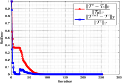
(a) Algorithm 1	(b) Algorithm 2

Figure 4: Convergence curves of Algorithm 1 and Algorithm 2.

2) Exact recovery: We then verify that the proposed t-CTV based TC and TRPCA model can achieve exact recovery for joint L+S tensors, as proved in our main theories.

For TC problem, we test on tensors $\mathcal{T}_{0}$ sized $N\times N\times 60\times 60$, with varying dimension $N=100,200,400$, and set the t-SVD rank $R$ as $0.05N,0.1N$ and $0.15N$. The sampling number $m$ is chosen by $4,3,2$ times of $d_{r}=R(2N-R)\times 60\times 60$, which can be viewed as a good quantity for reference. Table II reports the recovered tensors $\hat{\mathcal{T}}$s’ t-SVD ranks $\hat{R}$ and the corresponding RelErr $\|\hat{\mathcal{T}}-\mathcal{T}_{0}\|_{\mathrm{F}}/\|\mathcal{T}_{0}\|_{\mathrm{F}}$. Here, we consider three transforms: DFT, DCT, random orthogonal transform (DOT). The results reveal that t-CTV-TC obtains correct rank estimation and accurate recovery results,i.e., RelErr$\leq 10^{-5}$.

TABLE II: Performance of model (15) on synthetic tensors.

$N$	$R$	$\frac{m}{d_{r}}$	$p$	DFT		DCT		ROT
				$\hat{R}$	RelErr	$\hat{R}$	RelErr	$\hat{R}$	RelErr
100	5	4	0.39	5	4.54e-7	5	6.01e-6	5	4.73e-7
200	20	3	0.57	20	1.83e-7	20	3.30e-6	20	1.59e-7
400	60	2	0.56	60	2.90e-6	60	4.07e-6	60	8.92e-6

For the latter, consider $N\times N\times 60\times 60$ synthetic joint L+S tensor $\mathcal{T}_{0}$ varying $N=100$ and $200$ with $R=0.05N$, $0.1N$, and random sparse tensor $\mathcal{E}_{0}$ with sparsity $m=2\times 10^{6},8\times 10^{6}$ (corresponding sparsity ratio equals $5.56\%$). The tolerance to determine $\hat{\mathcal{E}}$’s sparsity is set as $0.001$. The recovered results are listed in Table III, showing that the recovery is correct with accurate rank/sparsity estimation, and tiny errors. This verifies the exact recovery guarantees.

TABLE III: Performance of model (16) on synthetic tensors.

$N$	$R$	$m$	DFT				DCT
			$\hat{R}$	RelErr$\mathcal{T}$	$\hat{m}$	RelErr$\mathcal{E}$	$\hat{R}$	RelErr$\mathcal{T}$	$\hat{m}$	RelErr$\mathcal{E}$
100	5	2e6	5	1.85e-7	2e6	2.46e-7	5	9.97e-6	2e6	1.14e-7
100	10	2e6	10	2.18e-6	2e6	3.96e-6	10	4.38e-7	2e6	7.27e-7
200	10	8e6	10	9.32e-7	8e6	9.84e-7	10	5.03e-7	8e6	3.64e-6
200	20	8e6	20	1.83e-6	8e6	3.03e-6	20	8.29e-6	8e6	7.10e-6

3) Phase transition and comparison to baselines: To further explore the ability of t-CTV based tensor recovery methods, we examine the recovery performance with varying t-SVD ranks of $\mathcal{T}_{0}$ from different sampling rates $p$ for the TC problem, and that with varying t-SVD ranks of $\mathcal{T}_{0}$ from different sparsity of $\mathcal{E}_{0}$ for the TRPCA task, respectively. Moreover, two baselines are considered for comparison, including the pure L prior model (order-$d$ TNN minimization [16][29]), and the L+S prior model (order-$d$ TNN plus anisotropic TV norm[25][28]). We omit those only considering the pure S priors since such models can hardly get comparable recovery results in such cases. The objective function of these baselines are listed in Table V.

For the TC task, we consider $\mathcal{T}_{0}$ sized $60\times 60\times 60\times 60$ and set t-SVD rank $R=[1:1:60]$ and random sampling rate $p=[0.01:0.01:1]$. For each $(R/N,p)$-pair, $N=60$, we simulate 30 test instances and declare a trail to be a success if the average RelErr of $\hat{\mathcal{T}}$ is less than $0.05$. Fig. 5 plots the phase transition diagrams (yellow=$100\%$, green=$0\%$), which evidently shows that t-CTV based TC model recovers more cases than TNN and TNN+TV models. Specially, compared with TNN+TV model, requiring to carefully tune the tradeoff parameter between L and S regularizers, t-CTV-TC entirely avoids this parameter setting issue.

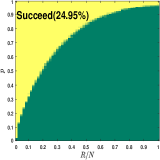
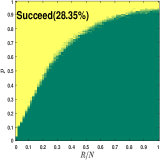
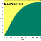
(a) TNN	(b) TNN+TV	(c) t-CTV

Figure 5: Phase transitions of t-CTV-TC model (15) with varying t-SVD ranks of $\mathcal{T}_{0}$ and sampling rates.

For the TRPCA task, we conduct tensor $\mathcal{T}_{0}$ in the same size with varying rank $R=[1:1:30]$. As for the sparse tensor $\mathcal{E}_{0}$, we vary its sparsity ratio $\rho_{s}={m}/{60^{4}}$ from $0.01$ to $0.50$ with interval $0.01$. Similarly, we simulate 30 times against each $(R/N,\rho_{s})$-pair for statistical stability. The corresponding fraction of correct recovery for TNN, TNN+TV and t-CTV-TRPCA are plotted in Fig. 6. It shows that t-CTV-TRPCA attains the best recovery ability with the correct area ratio $32.87\%$, evidently much higher than those obtained by TNN and TNN+TV baselines. Note that the TNN+TV model’s performance appears worse than the pure low-rank model. This can be rationally explained by that the TNN based TRPCA model has a solid recovery guarantee with determined parameter $\lambda$ [16], while the TNN+TV is not guaranteed in theory. Note that TNN+TV need to preset two model parameters, $\alpha$ and $\lambda$. In this phase transition experiment, we take $\lambda$ the same as that in the TNN model and carefully tune $\alpha$ from an appropriate range related to the smooth construction manner as aforementioned. By contrast, our t-CTV-TRPCA is parameter-free, and simultaneously with theoretical guarantees, making it easier and more reliable to be used in practice.

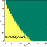
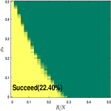
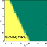
(a) TNN	(b) TNN+TV	(c) t-CTV

Figure 6: Phase transitions of t-CTV-TRPCA model (16) with varying t-SVD ranks of $\mathcal{T}_{0}$ and sparsity of $\mathcal{E}_{0}$.

7.2 Applications to Visual Data Inpainting

In this subsection, we apply the proposed t-CTV-TC method to the inpainting tasks for various visual tensor data and make comparison with SOTA tensor based methods considering L or L+S prior models, as listed in Table IV. Unless otherwise stated, all parameters involved in these competing methods are optimally assigned or selected as suggested in the reference papers. The peak signal-to-noise ratio (PSNR), structural similarity (SSIM [74]) and feature similarity (FSIM[75]) are employed to evaluate the recovery performance, all of which tends better performance with larger value.

1) Results on color images: We randomly select 50 RGB images from the USC-SIPI and BSD databases, of sizes $256\times 256\times 3$ and $321\times 481\times 3$, respectively. First, we test on the random element-wise sampling with sampling rate (SR) varying from $3\%$ to $80\%$. Table VI reports the inpainting results in terms of quantitative metrics on average. It is seen that our t-CTV method achieves the best performance in all evaluate criteria under all sampling cases. It can be seen that its advantage is more significant when SR is extremely low. As to the computational time, it can be seen that the average running time of proposed t-CTV is in the same order of magnitude as most of other methods (like SNN, KBR, TNN, SNN-TV, SPC-TV) and faster than several ones (like BCPF, IRTNN, MF-TV and TNN-TV). Fig. 7 shows the recovered images under SR=$10\%,20\%,40\%$ and $60\%$, revealing the recoveries obtained by our method are the closest to the ground truths. Considering its good recovery performance, it should be rational to say that the proposed method is efficient.

We further test the performance of all competing methods in extreme small sampling cases, when SR is set as $5\%$, $2\%$, $1\%$ and even $0.5\%$, meaning that $95\%$, $98\%$, $99\%$ and $99.5\%$ pixels are missing. Two typical cases are shown in Figs. 1 and 8, and our method evidently makes a relatively finer recovery while all other competing methods fail to a large extent. This verifies the result in Theorem 5 that t-CTV has a smaller lower sampling bound than conventional L and L+S models. As far as we know, there are no other methods capable of achieving similarly workable performance in such extreme cases for single image inpainting.

Last, we consider more challenging situations when the missing pixels are in structured masks including dead lines, wave lines, star patterns and text patterns. Some inpainting examples are depicted in Fig. 9. One can see that our method can still perform evidently superior beyond other competing peers. Especially, it’s known that the pure L prior models cannot estimate the missing entries when missing regions are some whole rows or columns [31]. As seen in Fig. 9, the SNN, BCPF, KBR, IRTNN and TNN methods are all invalid completely. In comparison, our t-CTV also uses the low-rank metric TNN in form, just instead defined on the gradient tensors. Yet it can finely process such extremely ill-possed cases. It also achieves better visualization results than those obtained by L+S prior models, showing its capability of delivering the two priors in its unique regularizer.

TABLE IV: Categories of related tensor completion methods.

Types	Methods
L	SNN[6], BCPF [38], KBR[30], IRTNN[51], TNN[29]
L$\&$S	MF-TV[20],SNN-TV[21],SPC-TV[23], TNN-TV[28]

TABLE V: Objectives of baseline TNN and TNN+TV models.

Types	TC	TRPCA
TNN	$\|\mathcal{T}\|_{\circledast,\mathfrak{L}}$	$\|\mathcal{T}\|_{\circledast,\mathfrak{L}}+\lambda\|\mathcal{E}\|_{1}$
TNN+TV	$\|\mathcal{T}\|_{\circledast,\mathfrak{L}}+\alpha\|\mathcal{T}\|_{\operatorname{TV}}$	$\|\mathcal{T}\|_{\circledast,\mathfrak{L}}+\alpha\|\mathcal{T}\|_{\operatorname{TV}}+\lambda\|\mathcal{E}\|_{1}$

TABLE VI: Color image inpainting performances of all competing methods under different sampling rates. Each result is averaged over all data. The best and second best result are highlighted in bold and underline, respectively. (/s: second).

SR	$3\%$			$5\%$			$10\%$			$20\%$		$40\%$		$60\%$		$80\%$		Time/s
Method	PSNR	SSIM	FSIM	PSNR	SSIM	FSIM	PSNR	SSIM	FSIM	PSNR	SSIM	PSNR	SSIM	PSNR	SSIM	PSNR	SSIM
SNN	15.99	0.292	0.654	17.21	0.365	0.690	19.62	0.498	0.752	22.71	0.674	27.28	0.859	31.48	0.944	36.59	0.983	10.49
BCPF	15.98	0.258	0.640	17.50	0.328	0.677	20.10	0.452	0.744	23.45	0.637	27.53	0.815	30.27	0.889	32.17	0.924	84.69
KBR	15.20	0.219	0.614	16.21	0.272	0.643	18.67	0.386	0.708	23.36	0.631	28.96	0.859	33.77	0.948	40.16	0.989	27.15
IRTNN	11.82	0.123	0.563	14.63	0.210	0.614	18.46	0.375	0.710	22.43	0.597	27.80	0.829	32.50	0.932	38.32	0.979	45.95
TNN	15.33	0.254	0.640	16.67	0.321	0.675	19.16	0.454	0.740	22.49	0.642	27.40	0.845	32.02	0.940	37.87	0.983	5.96
MF-TV	6.46	0.048	0.520	7.21	0.064	0.509	9.06	0.108	0.504	15.13	0.327	26.37	0.809	31.84	0.939	36.17	0.981	200.3
SNN-TV	16.73	0.432	0.600	18.31	0.498	0.658	21.79	0.657	0.753	24.48	0.789	28.47	0.909	32.08	0.960	36.59	0.987	14.28
SPC-TV	15.66	0.322	0.661	17.20	0.377	0.690	19.76	0.504	0.753	22.87	0.672	26.71	0.841	29.67	0.923	33.14	0.970	17.96
TNN-TV	17.66	0.460	0.613	19.32	0.532	0.668	21.16	0634	0.717	24.71	0.792	28.39	0.908	31.80	0.959	36.52	0.987	40.14
t-CTV	21.32	0.622	0.782	22.67	0.682	0.820	24.59	0.763	0.868	27.18	0.849	31.31	0.931	35.26	0.970	40.55	0.993	17.13

6.21/0.026	24.84/0.790	25.39/0.792	24.05/0.752	24.63/0.777	24.77/0.792	11.04/0.175	21.58/0.539	24.47/0.775	20.64/0.479	27.16/0.853	PSNR/SSIM
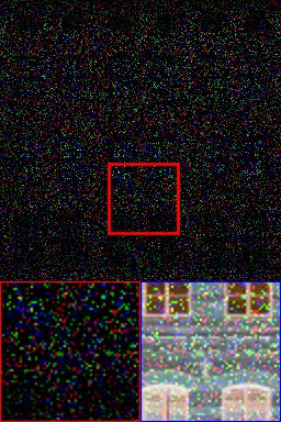
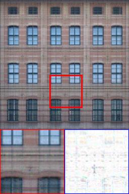
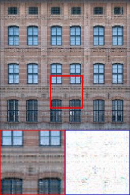
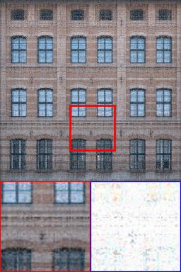
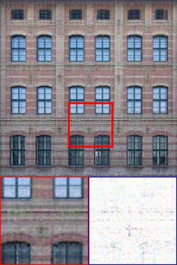
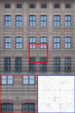
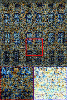
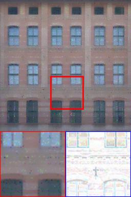
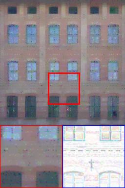
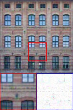
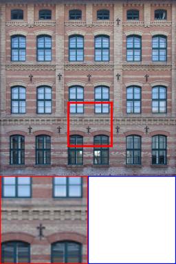
5.27/0.036	24.28/0.745	25.31/0.704	25.69/0.726	25.11/0.674	24.33/0.697	20.75/0.505	26.25/0.858	24.01/0.735	27.77/0.868	29.71/0.888	PSNR/SSIM
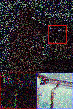
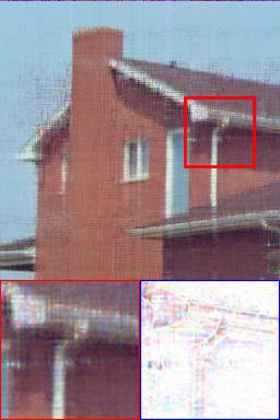
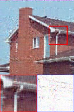
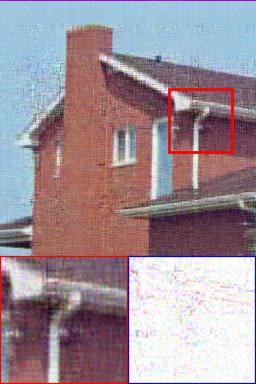
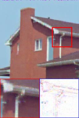
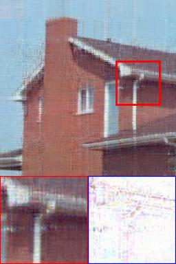
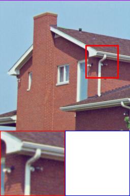
8.44/0.125	27.52/0.869	28.00/0.835	29.82/0.881	29.12/0.868	28.05/0.868	25.67/0.826	29.03/0.912	27.54/0.858	29.05/0.914	32.54/0.941	PSNR/SSIM
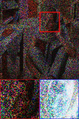
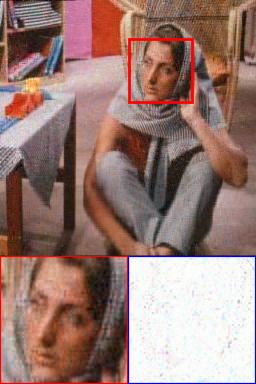
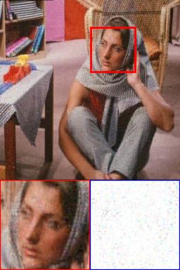
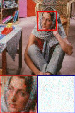
Observed	SNN	BCPF	KBR	IRTNN	TNN	MF-TV	SNN-TV	SPC-TV	TNN-TV	t-CTV	Ground truth

Figure 7: Color image inpainting results by all competing methods. From top to bottom: SR equals $10\%$, $20\%$, and $40\%$, respectively. For better viewing, we display the magnified map of a patch and corresponding error map (difference from the ground truth) under each image. Error maps with less color information indicate better restoration performance.

Observed	SNN	KBR	TNN	SNN-TV	SPC-TV	TNN-TV	t-CTV

Figure 8: Color image inpainting results obtained by all competing methods. From top to bottom: SR $=0.5\%,1\%,2\%,5\%$.

12.08/0.336	12.14/0.332	12.11/0.336	12.08/0.336	12.14/0.338	14.59/0.383	15.63/0.408	35.52/0.937	12.57/0.345	35.61/0.940	37.51/0.956	PSNR/SSIM
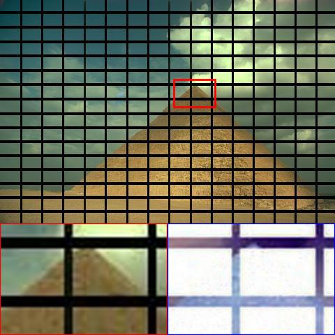
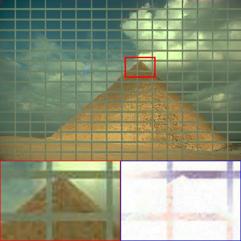
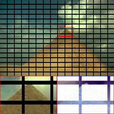
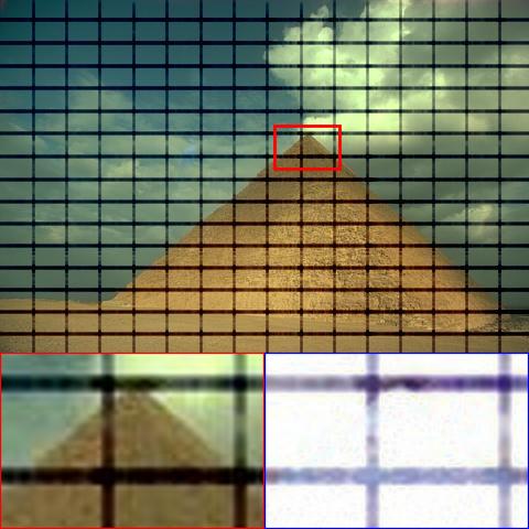
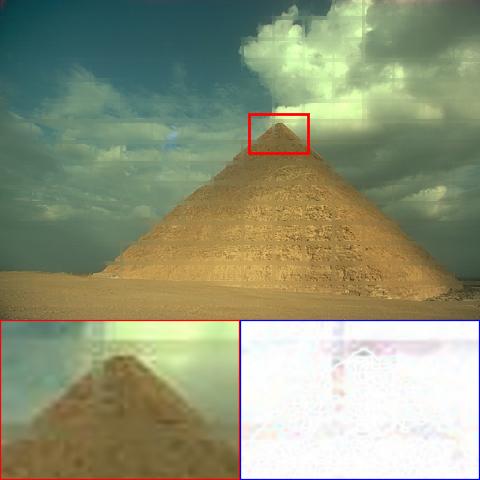
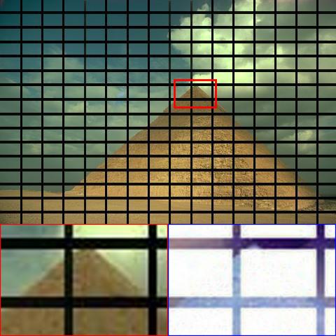
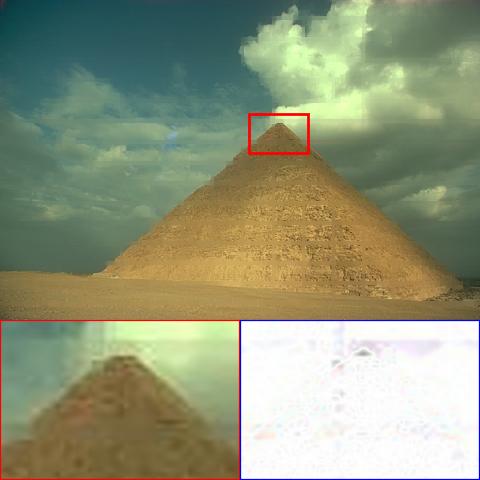
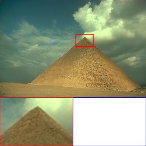
16.90/0.794	24.55/0.856	21.48/0.778	23.30/0.836	22.55/0.842	24.48/0.854	19.10/0.821	26.01/0.884	26.24/0.886	25.71/0.866	27.36/0.896	PSNR/SSIM
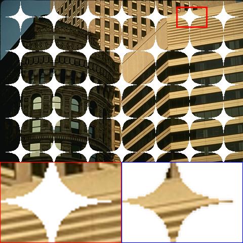
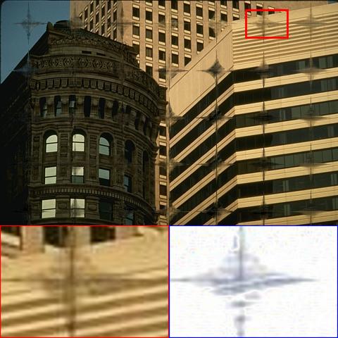
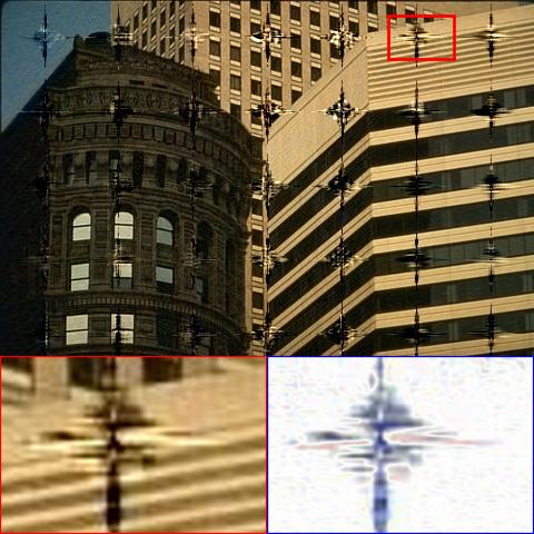
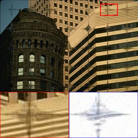
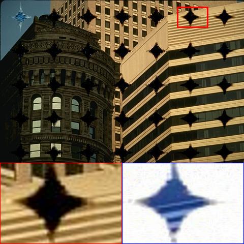
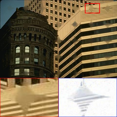
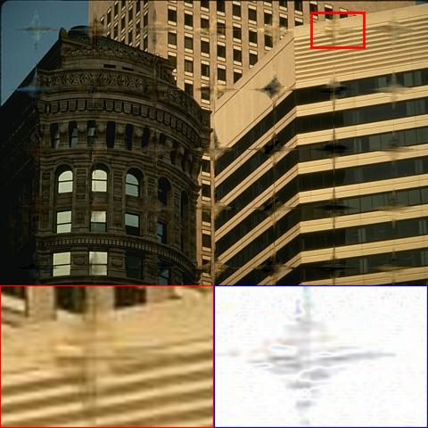
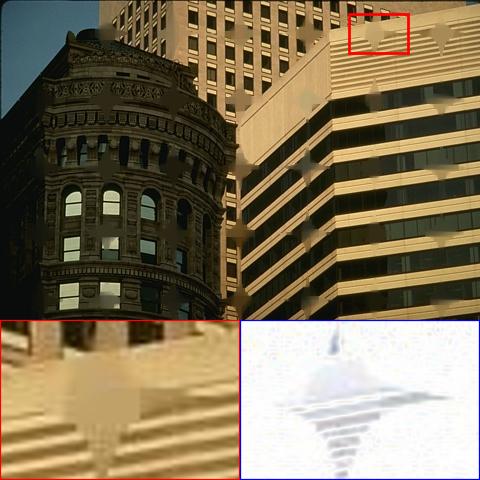
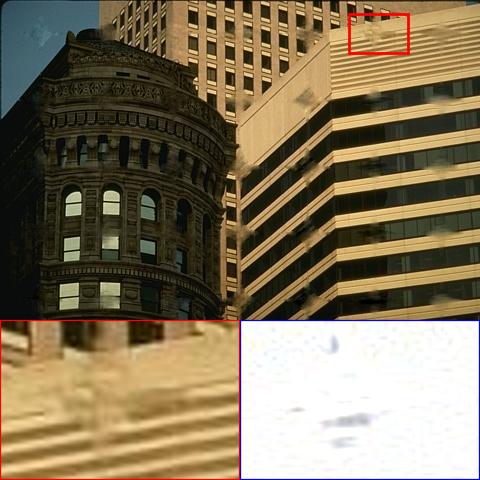
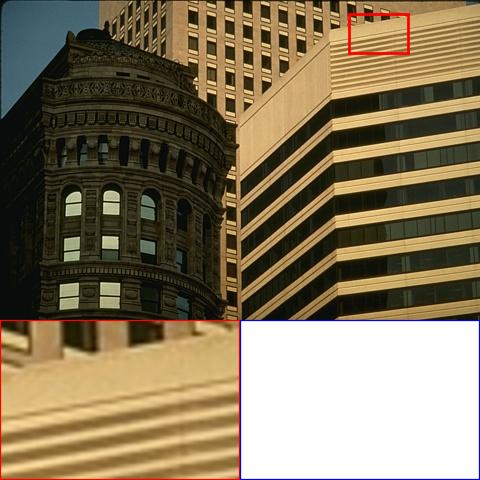
14.49/0.469	22.85/0.742	21.75/0.657	22.17/0.680	22.58/0.697	22.70/0.725	23.09/0.695	24.67/0.855	23.20/0.754	24.93/0.813	26.18/0.867	PSNR/SSIM
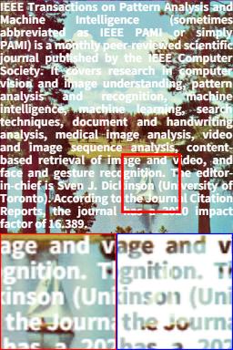
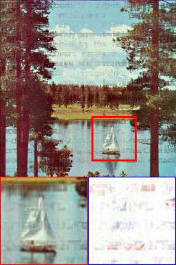
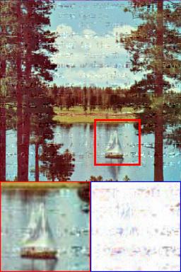
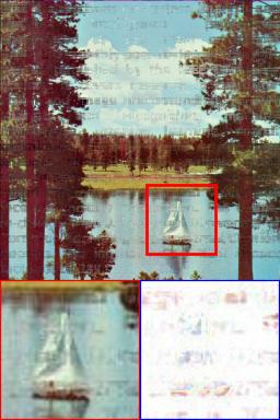
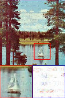
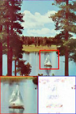
Observed	SNN	BCPF	KBR	IRTNN	TNN	MF-TV	SNN-TV	SPC-TV	TNN-TV	t-CTV	Ground truth

Figure 9: Color image inpainting results by all competing methods on three types of structured masked images.

(a) All SR cases	(b) SR $=10\%$

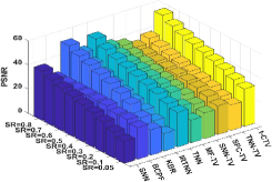
(a)

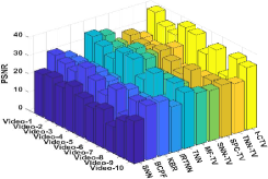
(b)

Figure 10: Performance comparison in terms of PSNR of recovered color videos obtained by all competing methods.

TABLE VII: ERGAS comparison of all competing methods on HSIs inpainting under SR $=5\%$.

Method	HSIs Data					Average
	Cuprite	DCMall	KSC	Pavia	PaviaU
SNN	153.6	451.4	240.0	411.0	374.9	326.2
BCPF	77.62	208.9	132.9	148.4	128.2	139.2
KBR	44.19	168.6	94.78	120.3	101.8	105.9
IRTNN	928.1	841.8	535.2	361.1	404.2	614.1
TNN	53.64	245.9	176.0	128.4	124.5	145.7
MF-TV	40.25	564.5	433.3	444.2	413.0	379.0
SNN-TV	135.7	453.0	211.0	361.6	321.8	296.6
SPC-TV	84.33	262.5	156.3	206.0	182.6	178.3
TNN-TV	127.4	422.9	205.0	305.8	286.6	269.6
t-CTV	25.16	119.9	75.73	70.01	59.91	70.15

9.47/0.017/1014	16.85/0.332/451.4	23.59/0.759/208.9	25.56/0.841/168.6
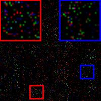
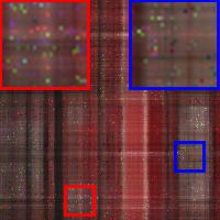
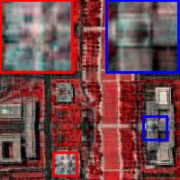
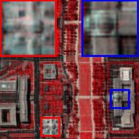
Observed	SNN	BCPF	KBR
11.45/0.095/841.8	22.49/0.717/245.9	18.18/0.491/564.5	16.85/0.244/453.0
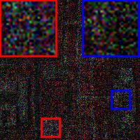
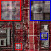
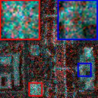
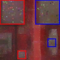
IRTNN	TNN	MF-TV	SNN-TV
21.64/0.675/262.5	17.44/0.291/422.9	29.04/0.929/119.9	PSNR/SSIM/ERGAS
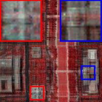
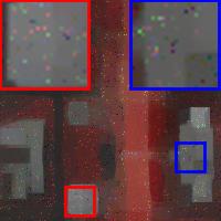
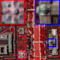
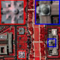
SPC-TV	TNN-TV	t-CTV	Ground truth

Figure 11: HSI inpainting results under SR $=5\%$. The displayed pseudo-color image uses bands 49-27-7 as R-G-B.

2) Results on color videos: In this experiment, we test all competing methods on 10 color video sequences from the YUV database. All videos are of size $176\times 144\times 3\times 200$. Note that the MF-TV and IRTNN methods cannot be directly used for order-4 tensors. One can reshape a video as $176\times 144\times 600$ or processing it frame-by-frame as an order-3 tensor. Since the former is very time-consuming and the performance of most methods on it is poor, we choose the latter in experiments. Fig. 10(a) plots the average PSNR values of different methods under different levels of SR, and Fig. 10(b) plots the detailed PSNR values of each recovered video using different methods when SR $=10\%$. Both bar graphs evidently show that our t-CTV method obtains the leading performance over other competing methods distinctly.

3) Results on hyperspectral images (HSIs): We choose five widely used HSIs, including Cuprite, DCMall, KSC, Pavia and Pavia university (PaviaU), in this experiment. All HSIs are preprocessed with size $200\times 200\times 50$. Similarly, we test the inpainting task under different levels of SR. Table VII lists the detailed recovery in terms of erreur relative globale adimensionnelle de synthese (ERGAS [76]) when SR $=5\%$. The smaller value of ERGAS indicates better restoration performance. Fig. 11 shows the pseudo-color image of the recovered HSIs via different methods. It is seen that our method performs better than all other competitors from the enlarged local area.

4) Results on more visual data in high-order tensor format: We then implement experiments on more visual data in tensor format, including order-$3$ CT and MRI medical images sized $256\times 256\times 127$, order-$4$ hyperspectral videos sized $188\times 120\times 33\times 31$ and order-$5$ light field images sized $216\times 324\times 3\times 17\times 17$. Table VIII lists the mean PSNR (MPSNR), mean SSIM (MSSIM) along with the third or more dimensions, and ERGAS values of the recovered data under SR $=10\%,30\%$ and $50\%$. These results consistently substantiate the advantages and potentials of our method for various high-order visual tensor data recovery. Results on some typical examples are shown in Fig. 12, Fig. 13 and Fig. 14 for better visualization. It should be indicated that all current competing methods take a relatively long running time in these tasks. Thus, exploring faster algorithms in handling high-order high-dimensional tensor should be a very meaningful topic in future research, e.g., parallelizing design [77], accelerating algorithm [78], and so on.

TABLE VIII: More data inpainting performances of all competing methods under different sampling rates. (/m: minute).

SR	Metric	SNN	KBR	TNN	SNN-TV	SPC-TV	TNN-TV	t-CTV
Order-$3$ CT$\&$MRI Medical Images
$10\%$	MPSNR	19.90	25.86	22.44	23.23	21.79	22.89	26.48
	MSSIM	0.533	0.710	0.458	0.716	0.478	0.675	0.839
	ERGAS	339.8	184.9	266.8	236.1	277.5	252.5	169.4
$30\%$	MPSNR	25.63	32.23	27.07	28.66	25.83	28.60	30.70
	MSSIM	0.766	0.896	0.699	0.870	0.632	0.875	0.879
	ERGAS	180.2	89.80	160.2	128.7	177.9	132.4	106.4
$50\%$	MPSNR	30.18	36.07	30.94	32.38	28.09	32.59	34.14
	MSSIM	0.892	0.952	0.839	0.934	0.726	0.937	0.940
	ERGAS	108.9	58.09	104.4	84.68	138.2	84.37	72.84
Time/m		7.41	17.08	4.11	11.25	53.29	17.24	17.96
Order-$4$ Hyperspectral Videos
$10\%$	MPSNR	25.47	33.34	41.13	28.90	35.69	28.26	44.70
	MSSIM	0.746	0.936	0.977	0.816	0.943	0.825	0.988
	ERGAS	148.5	60.01	24.56	100.1	45.86	107.6	16.23
$30\%$	MPSNR	33.79	49.07	48.41	35.96	37.62	36.87	50.89
	MSSIM	0.927	0.995	0.994	0.953	0.956	0.960	0.996
	ERGAS	56.97	9.824	10.59	44.41	36.71	39.98	7.956
$50\%$	MPSNR	38.99	54.44	52.89	41.15	39.31	42.10	54.18
	MSSIM	0.973	0.998	0.998	0.982	0.967	0.985	0.998
	ERGAS	31.33	5.293	6.369	24.44	30.25	21.92	5.448
Time/m		26.31	63.91	9.24	45.92	84.75	39.21	56.75
Order-$5$ Light Field Images
$10\%$	MPSNR	18.06	16.50	28.58	20.64	21.40	20.00	30.32
	MSSIM	0.554	0.379	0.800	0.748	0.627	0.742	0.871
	ERGAS	450.2	544.4	137.4	335.5	308.9	361.9	111.9
$30\%$	MPSNR	23.60	24.82	36.53	26.13	26.06	25.63	38.19
	MSSIM	0.761	0.780	0.945	0.892	0.747	0.890	0.965
	ERGAS	238.9	210.8	55.93	179.3	179.9	191.5	45.83
$50\%$	MPSNR	27.86	39.40	42.44	30.43	28.02	30.07	43.73
	MSSIM	0.884	0.982	0.981	0.948	0.803	0.947	0.987
	ERGAS	146.4	39.94	28.25	109.4	143.2	115.7	24.38
Time/m		77.21	202.8	27.70	640.24	417.5	99.61	128.5

Observed	KBR	TNN	SNN-TV	TNN-TV	t-CTV	Original

Figure 12: MRI and CT image inpainting results. From top to bottom: SR $=5\%,10\%$ and $20\%$.

25.47/0.746/148.5	33.34/0.936/60.01	41.13/0.977/24.56	28.90/0.816/100.1
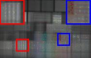
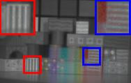
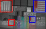
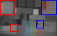
SNN	KBR	TNN	SNN-TV
35.69/0.943/45.86	28.26/0.825/107.6	44.70/0.988/16.23	PSNR/SSIM/ERGAS
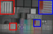
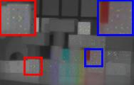
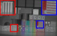
SPC-TV	TNN-TV	t-CTV	Ground truth

Figure 13: Hyperspectral video inpainting results under SR $=10\%$. The displayed pseudo-color image is the $7$-th frame of the recovered video with band 7-21-28 as R-G-B.

5.22/0.037/0.051	15.44/0.329/0.626	14.82/0.323/0.627	26.11/0.743/0.845	17.76/0.558/0.707	19.68/0.519/0.710	16.99/0.571/0.708	27.82/0.824/0.875	PSNR/SSIM/FSIM
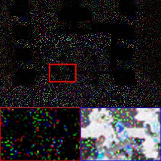
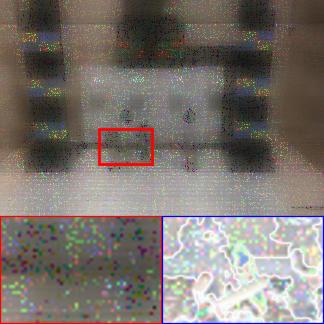
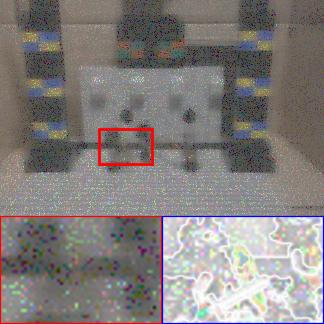
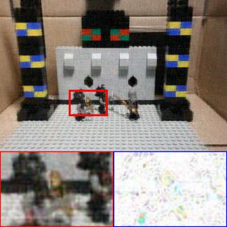
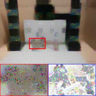
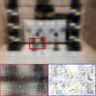
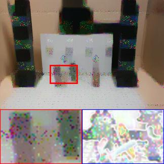
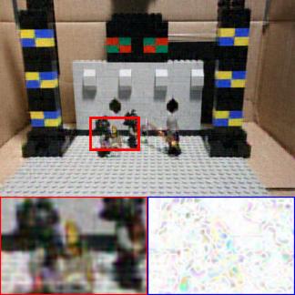
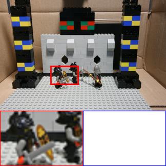
6.93/0.128/0.134	22.81/0.785/0.838	24.27/0.755/0.844	34.70/0.935/0.957	25.41/0.910/0.925	25.37/0.755/0.837	24.83/0.904/0.923	36.23/0.960/0.971	PSNR/SSIM/FSIM
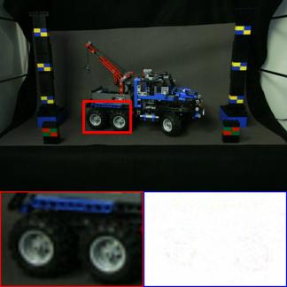
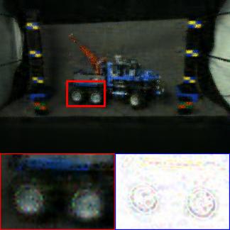
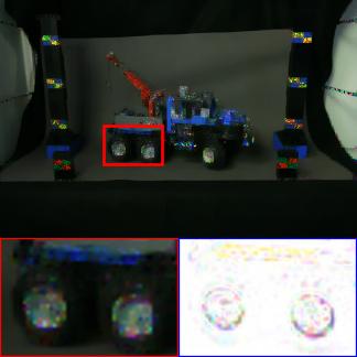
Observed	SNN	KBR	TNN	SNN-TV	SPC-TV	TNN-TV	t-CTV	Ground truth

Figure 14: Light field image inpainting results. From top to bottom: SR $=10\%$ and $30\%$. The displayed images are the $7$-th band and the $20$-th frame of the recovered LFIs.

7.3 Applications to Visual Data Denoising

We then apply the proposed t-CTV-TRPCA method to the denoising task. Similarly, we compare our results with related L and L+S modeling methods, summarized in Table IX. Note that there exist multiple parameters in these competing methods. We choose the suggested parameter setting in corresponding release codes. In comparison, our t-CTV-RPCA method doesn’t need to tune parameters where the sole parameter $\lambda$ is set as $1/\sqrt{n_{(1)}\ell}$ given by Theorem 6.

TABLE IX: Categories of related tensor RPCA methods.

Types	Methods
L	SNN[7], TNN[16], KBR[30]
L$\&$S	LRTV[22], LRTDTV[24], TLR-HTV/TLR-SSTV[25]

TABLE X: Visual data denoising performances of all competing methods under different levels of noise.

Noise	S = 0.1			S = 0.2			S = 0.3			S = 0.4			S = 0.1, G = 0.05			S = 0.2, G = 0.05			Time/s
Method	PSNR	SSIM	FSIM	PSNR	SSIM	FSIM	PSNR	SSIM	FSIM	PSNR	SSIM	FSIM	PSNR	SSIM	FSIM	PSNR	SSIM	FSIM
Order-$3$ Color Images
SNN	25.65	0.826	0.878	24.68	0.789	0.858	23.69	0.746	0.837	22.64	0.691	0.813	24.39	0.708	0.840	23.60	0.669	0.823	16.60
TNN	29.85	0.923	0.944	28.16	0.871	0.922	25.92	0.748	0.877	21.97	0.479	0.767	25.92	0.672	0.857	24.30	0.588	0.820	9.18
KBR	25.57	0.819	0.883	24.31	0.763	0.856	22.86	0.677	0.822	21.28	0.548	0.770	24.13	0.690	0.841	23.00	0.634	0.816	29.81
LRTV	28.35	0.807	0.927	24.33	0.624	0.849	21.25	0.467	0.762	18.77	0.346	0.677	26.07	0.681	0.863	23.15	0.545	0.796	11.24
LRTDTV	29.49	0.845	0.929	25.47	0.698	0.859	22.30	0.539	0.775	19.65	0.398	0.692	26.78	0.729	0.875	23.97	0.607	0.814	11.21
TLR-HTV	31.64	0.893	0.949	25.79	0.660	0.861	17.82	0.309	0.659	11.70	0.111	0.469	26.14	0.659	0.854	21.85	0.472	0.758	12.62
t-CTV	31.65	0.933	0.960	30.56	0.913	0.949	29.36	0.884	0.935	27.97	0.836	0.914	28.20	0.774	0.891	27.25	0.733	0.872	18.20
Order-$3$ Hyperspectral Images
SNN	42.78	0.976	0.978	40.60	0.974	0.985	37.86	0.970	0.974	34.49	0.948	0.964	31.36	0.920	0.952	30.26	0.907	0.946	80.80
TNN	44.57	0.991	0.993	42.73	0.988	0.992	40.29	0.982	0.988	36.30	0.955	0.976	29.55	0.747	0.904	28.19	0.690	0.881	77.87
KBR	36.39	0.971	0.979	35.38	0.966	0.975	33.94	0.957	0.968	32.32	0.924	0.949	32.90	0.925	0.956	32.01	0.913	0.950	161.7
LRTV	38.01	0.978	0.988	36.06	0.962	0.979	34.10	0.933	0.964	32.15	0.890	0.941	32.22	0.898	0.940	32.20	0.879	0.929	12.89
LRTDTV	39.63	0.978	0.990	38.75	0.975	0.988	37.45	0.968	0.984	35.66	0.953	0.975	35.20	0.930	0.963	34.30	0.918	0.956	53.22
TLR-SSTV	37.68	0.973	0.983	36.09	0.962	0.976	34.42	0.946	0.966	32.75	0.923	0.951	31.72	0.855	0.928	31.04	0.841	0.917	23.94
t-CTV	46.32	0.993	0.996	44.93	0.992	0.995	43.27	0.989	0.993	41.37	0.985	0.991	33.01	0.871	0.940	32.28	0.843	0.927	118.0
Order-$4$ Color Videos
SNN	21.50	0.696	0.797	20.70	0.666	0.779	19.82	0.634	0.762	18.82	0.600	0.744	20.60	0.642	0.772	19.91	0.618	0.759	278.3
TNN	37.31	0.982	0.986	35.49	0.971	0.980	33.29	0.939	0.965	28.94	0.789	0.907	28.00	0.694	0.868	26.35	0.624	0.834	188.2
KBR	29.52	0.906	0.938	28.72	0.896	0.931	27.71	0.878	0.920	25.99	0.836	0.894	28.35	0.844	0.914	27.45	0.825	0.904	267.5
LRTV	31.03	0.851	0.943	23.64	0.543	0.804	19.69	0.362	0.681	16.94	0.252	0.582	26.48	0.649	0.835	22.23	0.462	0.735	64.30
LRTDTV	32.91	0.905	0.958	28.80	0.806	0.909	25.32	0.673	0.839	22.24	0.510	0.742	29.37	0.806	0.908	26.55	0.702	0.857	174.1
TLR-SSTV	36.23	0.969	0.981	34.25	0.949	0.971	31.45	0.894	0.948	27.54	0.758	0.889	29.27	0.772	0.900	27.75	0.715	0.873	177.3
t-CTV	39.73	0.987	0.990	38.17	0.982	0.987	36.62	0.974	0.983	34.85	0.959	0.974	30.90	0.817	0.910	29.79	0.779	0.891	260.4

12.13/0.144/0.583	24.51/0.844/0.855/	27.54/0.891/0.926	24.73/0.844/0.873	25.57/0.773/0.870	27.25/0.785/0.902	28.14/0.813/0.923	29.38/0.944/0.951	PSNR/SSIM/FSIM
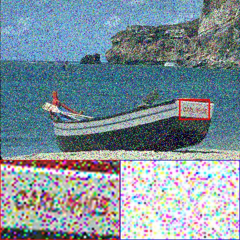
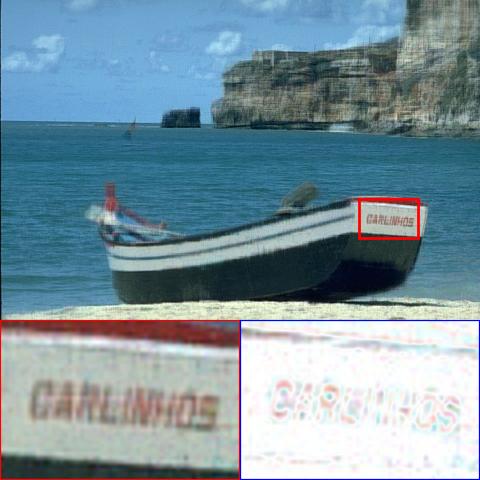
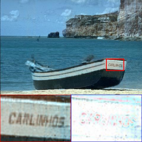
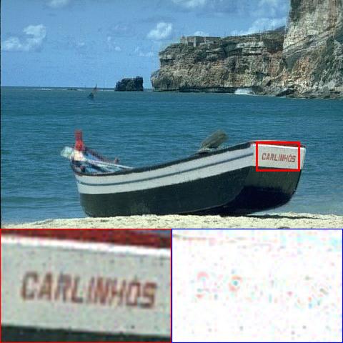
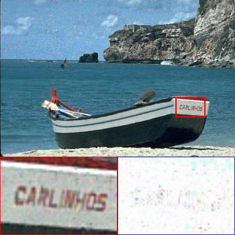
8.57/0.087/0.434	21.10/0.601/0.792	18.23/0.348/0.687	18.99/0.457/0.714	20.62/0.554/0.761	23.90/0.734/0.844	21.20/0.512/0.776	26.92/0.878/0.922	PSNR/SSIM/FSIM
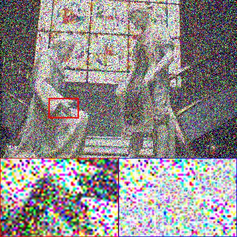
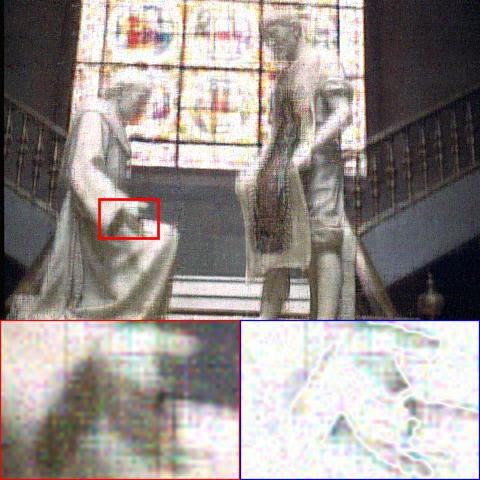
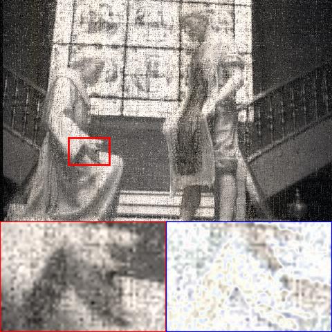
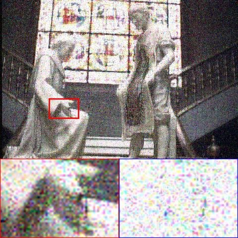
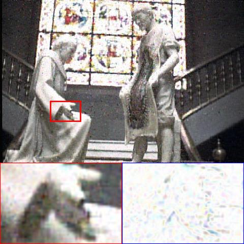
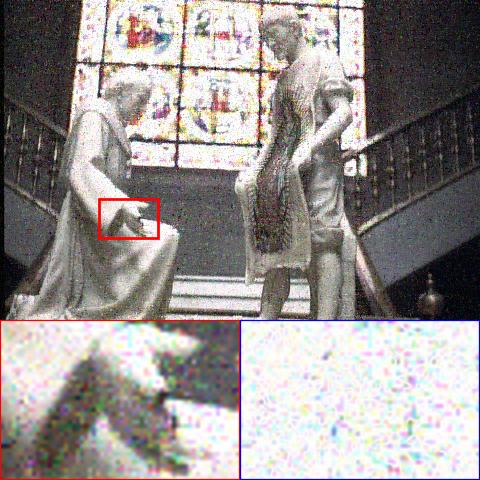
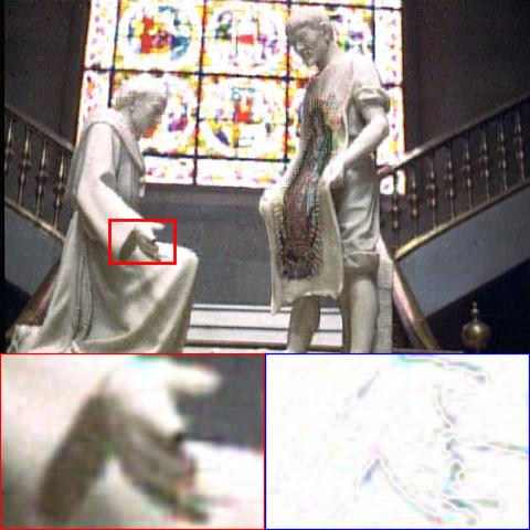
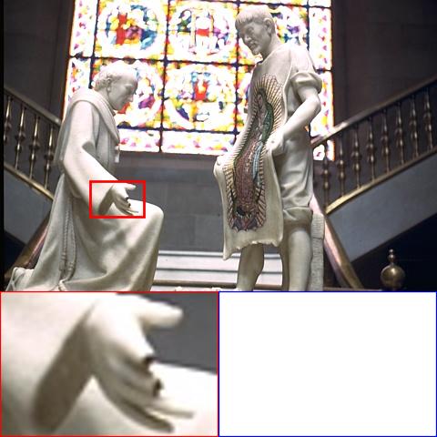
11.56/0.171/0.555	22.97/0.615/0.819	22.89/0.582/0.814	21.38/0.642/0.823	24.10/0.697/0.854	23.39/0.721/0.858	23.27/0.604/0.823	26.02/0.739/0.870	PSNR/SSIM/FSIM
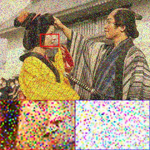
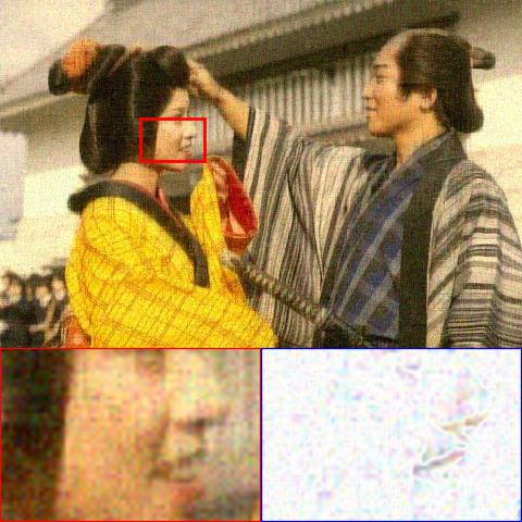
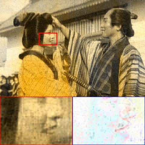
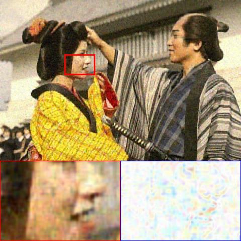
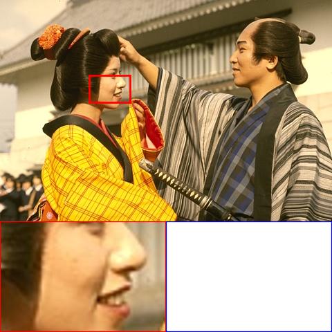
Noisy	SNN	KBR	TNN	LRTV	LRTDTV	TLR-HTV	t-CTV	Ground truth

Figure 15: Color image denoising results by all competing methods. From top to bottom: cases containing sparse noise of noise percentages $0.2$ and $0.4$, images containing mixed noise with sparse noise with noise percentage $0.2$ and Gaussian noise with zero-mean and standard deviation $0.05$.

8.10/0.017/1872	35.87/0.933/89.24	36.31/0.931/77.79
Noisy	SNN	KBR
33.10/0.913/102.9	32.93/0.846/109.5	36.87/0.943/64.49
TNN	LRTV	LRTDTV
33.87/0.909/92.33	42.38/0.980/44.94	PSNR/SSIM/ERGAS
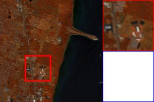
TLR-SSTV	t-CTV	Ground truth

Figure 16: HSI “KSC” denoising results on a typical HSI containing sparse noise with noise percentage $0.4$.

10.49/0.098/0.455	21.86/0.770/0.825	32.96/0.952/0.967	38.14/0.964/0.987	29.85/0.809/0.912	31.03/0.869/0.947	32.66/0.936/0.964	41.76/0.986/0.993	PSNR/SSIM/FSIM
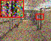
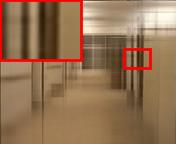
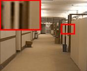
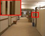
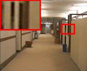
8.67/0.078/0.399	18.59/0.683/0.771	26.49/0.902/0.922	32.70/0.924/0.965	24.75/0.735/0.850	26.92/0.882/0.919	28.94/0.914/0.943	36.92/0.987/0.990	PSNR/SSIM/FSIM
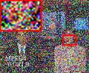
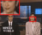
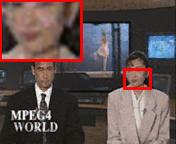
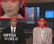
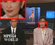
Noisy	SNN	KBR	TNN	LRTV	LRTDTV	TLR-SSTV	t-CTV	Ground truth

Figure 17: Color video denoising results by all competing methods. From top to bottom: cases containing sparse noise with noise percentage $0.3,0.4$.

We use the aforementioned databases of color images, HSIs and color videos for test. In Table X, we list the denoising results on sparse salt and pepper noise (S) with different percentages, and their mixed noise with a bit Gaussian noise (G) with zero-mean and standard deviation $0.05$. From this table, we can find easily that our t-CTV based method achieves the best performance in all sparse noise cases. Especially, when the percentage of sparse noise is getting increased, our leading advantages are clearer. For example, our method is almost 5dB in PSNR higher than the second-best method when $40\%$ percentage pixels are corrupted by sparse noise.

As for mixed noise cases, our method also shows competitive performance. It should be indicated that our t-CTV-TRPCA model is only a generic model imposing $L_{1}$ norm on noise elements succeeding from conventional RPCA models, specifically suitable for sparse noises in nature. The purpose of considering some Gaussian noise is to test our model’s stability. For these related methods including LRTV, LRTDTV and TLR-HTV/SSTV, their models include extra $L_{2}$-norm element, and thus is formulated appropriate for mixed Gaussian noises. From the results of Table X, it can be observed that our method can overmatch other competitors even without such explicit Gaussian noise item, revealing the powerfulness of such regularization term on expressing natural visual tensors with L+S priors.

We further display several typical recovered examples for visualization comparison in Fig. 15, Fig. 16 and Fig. 17. From these figures, it can be easily seen that our t-CTV based method achieves better noise removal performance. Specifically, the denoising results by our method maintain clearer outlines and more faithful local details compared with other competitors, validating its fine capability in extracting the natural images with intrinsic L+S structures.

8 Conclusion

In this study, we have proposed a new regularization term, called t-CTV, to encode both L+S priors, commonly possessed by natural visual tensor data, into a unique concise form. By formulating the regularization in two typical tensor recovery tasks, including TC and TRPCA, we can prove their exact recovery guarantee theoretically for both models. This should be the first theoretical exact recovery result along this L+S prior modeling research, revealing its general reliability and potential usefulness of the proposed regularizer. We also prove that such L+S modeling manner is with a lower sampling complexity bound beyond conventional L and/or S prior models, which has been comprehensively validated by our experiments in different types of practical visual tensor data. Especially, even under the extremely low sampling rage $0.5\%$, our method can still get an acceptable recovery effect, when all other competing methods totally fail in such cases. We’ll try to testify more tensor recovery tasks, like outlier detection and background extraction, by combining this regularizer into their corresponding models to further validate its effect, and attempt to explore more targeted theory for further revealing its working insights in our future investigations. Furthermore, it is also meaningful to extend the theoretical and algorithmic explorations of this work to other ones with low-rank regularizers under different matrix/tensor transformations in our future research.

Hailin Wang is currently pursuing a Ph.D. degree with the School of Mathematics and Statistics, Xi’an Jiaotong University, Xi’an, China. He received the B.Sc and M.Sc degree in statistic from Southwest University, Chongqing, China, in 2019, 2021, respectively. His research interests include compressed sensing and low-rank matrix/tensor analysis.

Jiangjun Peng received the B.Sc degree in mathematical from Northwest University, Xi’an, China, in 2015 and the M.Sc degree in mathematics from Xi’an Jiaotong University, Xi’an, China, in 2018. He was a researcher in Tencent from 2018 to 2020. He is currently pursuing a Ph.D. degree with the School of Mathematics and Statistics, Xi’an Jiaotong University, Xi’an. His current research interests include low-rank matrix/tensor analysis, theoretical machine learning and model-driven deep learning.

Wenjin Qin is currently pursuing a Ph.D. degree with the School of Mathematics and Statistics, Southwest University, Chongqing, China. He received the B.Sc degree in applied statistics from Hechi University, Guangxi, China, in 2019, and the M.Sc degree in statistic from Southwest University, Chongqing, China, in 2022. His research interests include deep learning, compressed sensing, low-rank matrix recovery and tensor sparsity.

Jianjun Wang (Member, IEEE) received the B.Sc degree in mathematical education from Ningxia University in 2000 and the M.Sc degree in fundamental mathematics in 2003 from Ningxia University, China, and Ph.D degree in applied mathematics from the Institute for Information and System Science, Xi’an Jiaotong University in 2006. He is currently a professor in the School of Mathematics and Statistics, Southwest University, Chongqing, China. His research focus on machine learning, data mining, neural networks and sparse learning. He is a member of the IEEE.

Deyu Meng (Member, IEEE) received the B.Sc., M.Sc., and Ph.D. degrees from Xi’an Jiaotong University, Xi’an, China, in 2001, 2004, and 2008, respectively. From 2012 to 2014, he took his two-year sabbatical leave at Carnegie Mellon University, Pittsburgh, PA, USA. He is a Professor with the School of Mathematics and Statistics, Xi’an Jiaotong University, and an Adjunct Professor with the Faculty of Information Technology, Macau University of Science and Technology, Taipa, Macau, China. His research interests include model-based deep learning, variational networks, and meta learning.

References

- [1] P. McCullagh, Tensor methods in statistics. Chapman and Hall/CRC, 2018.
- [2] A. Cichocki, D. Mandic, L. De Lathauwer, G. Zhou, Q. Zhao, C. Caiafa, and H. A. Phan, “Tensor decompositions for signal processing applications: From two-way to multiway component analysis,” IEEE Signal Process. Mag., vol. 32, no. 2, pp. 145–163, 2015.
- [3] E. E. Papalexakis, C. Faloutsos, and N. D. Sidiropoulos, “Tensors for data mining and data fusion: Models, applications, and scalable algorithms,” ACM Trans. Intell. Syst. Technol., vol. 8, no. 2, pp. 1–44, 2016.
- [4] M. Signoretto, Q. Tran Dinh, L. De Lathauwer, and J. A. Suykens, “Learning with tensors: a framework based on convex optimization and spectral regularization,” Mach. Learn., vol. 94, no. 3, pp. 303–351, 2014.
- [5] Y. Panagakis, J. Kossaifi, G. G. Chrysos, J. Oldfield, M. A. Nicolaou, A. Anandkumar, and S. Zafeiriou, “Tensor methods in computer vision and deep learning,” Proceedings of the IEEE, vol. 109, no. 5, pp. 863–890, 2021.
- [6] J. Liu, P. Musialski, P. Wonka, and J. Ye, “Tensor completion for estimating missing values in visual data,” IEEE Trans. Pattern Anal. Mach. Intell., vol. 35, no. 1, pp. 208–220, 2012.
- [7] B. Huang, C. Mu, D. Goldfarb, and J. Wright, “Provable models for robust low-rank tensor completion,” Pac. J. Optim., vol. 11, no. 2, pp. 339–364, 2015.
- [8] F. L. Hitchcock, “The expression of a tensor or a polyadic as a sum of products,” Int. J. Math. Phys., vol. 6, no. 1-4, pp. 164–189, 1927.
- [9] L. R. Tucker, “Implications of factor analysis of three-way matrices for measurement of change,” Problems in Measuring Change, vol. 15, no. 122-137, p. 3, 1963.
- [10] L. De Lathauwer, B. De Moor, and J. Vandewalle, “A multilinear singular value decomposition,” SIAM J. Matrix Anal. Appl., vol. 21, no. 4, pp. 1253–1278, 2000.
- [11] I. Oseledets, “Tensor-train decomposition,” SIAM J. Sci. Comput., vol. 33, no. 5, pp. 2295–2317, 2011.
- [12] Q. Zhao, G. Zhou, S. Xie, L. Zhang, and A. Cichocki, “Tensor ring decomposition,” arXiv: Numerical Analysis, arXiv: 1606.05535, 2016.
- [13] M. E. Kilmer and C. D. Martin, “Factorization strategies for third-order tensors,” Linear Alg. Appl., vol. 435, no. 3, pp. 641–658, 2011.
- [14] M. E. Kilmer, L. Horesh, H. Avron, and E. Newman, “Tensor-tensor algebra for optimal representation and compression of multiway data,” Proc Natl Acad Sci U S A., vol. 118, no. 28, 2021.
- [15] Z. Zhang and S. Aeron, “Exact tensor completion using t-SVD,” IEEE Trans. Signal Process., vol. 65, no. 6, pp. 1511–1526, 2016.
- [16] C. Lu, J. Feng, Y. Chen, W. Liu, Z. Lin, and S. Yan, “Tensor robust principal component analysis with a new tensor nuclear norm,” IEEE Trans. Pattern Anal. Mach. Intell., vol. 42, no. 4, pp. 925–938, 2019.
- [17] F. Zhang, J. Wang, W. Wang, and C. Xu, “Low-tubal-rank plus sparse tensor recovery with prior subspace information,” IEEE Trans. Pattern Anal. Mach. Intell., vol. 43, no. 10, pp. 3492–3507, 2020.
- [18] J. Hou, F. Zhang, H. Qiu, J. Wang, Y. Wang, and D. Meng, “Robust low-tubal-rank tensor recovery from binary measurements,” IEEE Trans. Pattern Anal. Mach. Intell., 2021.
- [19] X. Zhang and M. K.-P. Ng, “Low rank tensor completion with poisson observations,” IEEE Trans. Pattern Anal. Mach. Intell., 2021.
- [20] T.-Y. Ji, T.-Z. Huang, X.-L. Zhao, T.-H. Ma, and G. Liu, “Tensor completion using total variation and low-rank matrix factorization,” Inf. Sci., vol. 326, pp. 243–257, 2016.
- [21] X. Li, Y. Ye, and X. Xu, “Low-rank tensor completion with total variation for visual data inpainting,” in AAAI, vol. 31, no. 1, 2017.
- [22] W. He, H. Zhang, L. Zhang, and H. Shen, “Total-variation-regularized low-rank matrix factorization for hyperspectral image restoration,” IEEE Trans. Geosci. Remote Sens., vol. 54, no. 1, pp. 178–188, 2015.
- [23] T. Yokota, Q. Zhao, and A. Cichocki, “Smooth parafac decomposition for tensor completion,” IEEE Trans. Image Process., vol. 64, no. 20, pp. 5423–5436, 2016.
- [24] Y. Wang, J. Peng, Q. Zhao, Y. Leung, X.-L. Zhao, and D. Meng, “Hyperspectral image restoration via total variation regularized low-rank tensor decomposition,” IEEE J. Sel. Topics Appl. Earth Observ. Remote Sens., vol. 11, no. 4, pp. 1227–1243, 2017.
- [25] Y. Chen, S. Wang, and Y. Zhou, “Tensor nuclear norm-based low-rank approximation with total variation regularization,” IEEE J. Sel. Topics Signal Process., vol. 12, no. 6, pp. 1364–1377, 2018.
- [26] H. Zhang, L. Liu, W. He, and L. Zhang, “Hyperspectral image denoising with total variation regularization and nonlocal low-rank tensor decomposition,” IEEE Trans. Geosci. Remote Sens., vol. 58, no. 5, pp. 3071–3084, 2019.
- [27] C.-Y. Ko, K. Batselier, L. Daniel, W. Yu, and N. Wong, “Fast and accurate tensor completion with total variation regularized tensor trains,” IEEE Trans. Image Process., vol. 29, pp. 6918–6931, 2020.
- [28] D. Qiu, M. Bai, M. K. Ng, and X. Zhang, “Robust low-rank tensor completion via transformed tensor nuclear norm with total variation regularization,” Neurocomputing, vol. 435, pp. 197–215, 2021.
- [29] W. Qin, H. Wang, F. Zhang, J. Wang, X. Luo, and T. Huang, “Low-rank high-order tensor completion with applications in visual data,” IEEE Trans. Image Process., vol. 31, pp. 2433–2448, 2022.
- [30] Q. Xie, Q. Zhao, D. Meng, and Z. Xu, “Kronecker-basis-representation based tensor sparsity and its applications to tensor recovery,” IEEE Trans. Pattern Anal. Mach. Intell., vol. 40, no. 8, pp. 1888–1902, 2017.
- [31] E. J. Candès and B. Recht, “Exact matrix completion via convex optimization,” Found. Comput. Math., vol. 9, no. 6, pp. 717–772, 2009.
- [32] E. J. Candès, X. Li, Y. Ma, and J. Wright, “Robust principal component analysis?” J. ACM, vol. 58, no. 3, pp. 1–37, 2011.
- [33] D. Goldfarb and Z. Qin, “Robust low-rank tensor recovery: Models and algorithms,” SIAM J. Matrix Anal. Appl., vol. 35, no. 1, pp. 225–253, 2014.
- [34] B. Romera-Paredes and M. Pontil, “A new convex relaxation for tensor completion,” in NIPS, vol. 26, 2013.
- [35] C. Mu, B. Huang, J. Wright, and D. Goldfarb, “Square deal: Lower bounds and improved relaxations for tensor recovery,” in ICML, 2014, pp. 73–81.
- [36] X. Zhang, “A nonconvex relaxation approach to low-rank tensor completion,” IEEE Trans. Neural Netw. Learn. Syst., vol. 30, no. 6, pp. 1659–1671, 2018.
- [37] Y. Xu, R. Hao, W. Yin, and Z. Su, “Parallel matrix factorization for low-rank tensor completion,” Inverse Probl. Imaging, vol. 9, no. 2, pp. 601–624, 2015.
- [38] Q. Zhao, L. Zhang, and A. Cichocki, “Bayesian CP factorization of incomplete tensors with automatic rank determination,” IEEE Trans. Pattern Anal. Mach. Intell., vol. 37, no. 9, pp. 1751–1763, 2015.
- [39] A. Anandkumar, P. Jain, Y. Shi, and U. N. Niranjan, “Tensor vs. matrix methods: Robust tensor decomposition under block sparse perturbations,” in Artificial Intelligence and Statistics. PMLR, 2016, pp. 268–276.
- [40] Q. Zhao, G. Zhou, L. Zhang, A. Cichocki, and S.-I. Amari, “Bayesian robust tensor factorization for incomplete multiway data,” IEEE Trans. Neural Netw. Learn. Syst., vol. 27, no. 4, pp. 736–748, 2015.
- [41] J. A. Bengua, H. N. Phien, H. D. Tuan, and M. N. Do, “Efficient tensor completion for color image and video recovery: Low-rank tensor train,” IEEE Trans. Image Process., vol. 26, no. 5, pp. 2466–2479, 2017.
- [42] H. Rauhut, R. Schneider, and Ž. Stojanac, “Low rank tensor recovery via iterative hard thresholding,” Linear Alg. Appl., vol. 523, pp. 220–262, 2017.
- [43] W. Wang, V. Aggarwal, and S. Aeron, “Efficient low rank tensor ring completion,” in ICCV, 2017, pp. 5697–5705.
- [44] Y.-B. Zheng, T.-Z. Huang, X.-L. Zhao, Q. Zhao, and T.-X. Jiang, “Fully-connected tensor network decomposition and its application to higher-order tensor completion,” in AAAI, vol. 35, no. 12, 2021, pp. 11 071–11 078.
- [45] M. E. Kilmer, K. Braman, N. Hao, and R. C. Hoover, “Third-order tensors as operators on matrices: A theoretical and computational framework with applications in imaging,” SIAM J. Matrix Anal. Appl., vol. 34, no. 1, pp. 148–172, 2013.
- [46] O. Semerci, N. Hao, M. E. Kilmer, and E. L. Miller, “Tensor-based formulation and nuclear norm regularization for multienergy computed tomography,” IEEE Trans. Image Process., vol. 23, no. 4, pp. 1678–1693, 2014.
- [47] C. Lu, X. Peng, and Y. Wei, “Low-rank tensor completion with a new tensor nuclear norm induced by invertible linear transforms,” in CVPR, 2019, pp. 5996–6004.
- [48] X.-Y. Liu, S. Aeron, V. Aggarwal, and X. Wang, “Low-tubal-rank tensor completion using alternating minimization,” IEEE Trans. Inf. Theory, vol. 66, no. 3, pp. 1714–1737, 2019.
- [49] Q. Jiang and M. Ng, “Robust low-tubal-rank tensor completion via convex optimization.” in IJCAI, 2019, pp. 2649–2655.
- [50] H. Wang, F. Zhang, J. Wang, and Y. Wang, “Estimating structural missing values via low-tubal-rank tensor completion,” in ICASSP. IEEE, 2020, pp. 3297–3301.
- [51] H. Wang, F. Zhang, J. Wang, T. Huang, J. Huang, and X. Liu, “Generalized nonconvex approach for low-tubal-rank tensor recovery,” IEEE Trans. Neural Netw. Learn. Syst., 2021.
- [52] C. D. Martin, R. Shafer, and B. LaRue, “An order-p tensor factorization with applications in imaging,” SIAM J. Sci. Comput., vol. 35, no. 1, pp. A474–A490, 2013.
- [53] E. Kernfeld, M. Kilmer, and S. Aeron, “Tensor–tensor products with invertible linear transforms,” Linear Alg. Appl., vol. 485, pp. 545–570, 2015.
- [54] L. I. Rudin, S. Osher, and E. Fatemi, “Nonlinear total variation based noise removal algorithms,” Physica D, vol. 60, no. 1-4, pp. 259–268, 1992.
- [55] A. Chambolle and P.-L. Lions, “Image recovery via total variation minimization and related problems,” Numer. Math., vol. 76, no. 2, pp. 167–188, 1997.
- [56] A. Beck and M. Teboulle, “Fast gradient-based algorithms for constrained total variation image denoising and deblurring problems,” IEEE Trans. Image Process., vol. 18, no. 11, pp. 2419–2434, 2009.
- [57] Y. Wang, J. Yang, W. Yin, and Y. Zhang, “A new alternating minimization algorithm for total variation image reconstruction,” SIAM J. Imaging Sci., vol. 1, no. 3, pp. 248–272, 2008.
- [58] Q. Yuan, L. Zhang, and H. Shen, “Hyperspectral image denoising employing a spectral–spatial adaptive total variation model,” IEEE Trans. Geosci. Remote Sens., vol. 50, no. 10, pp. 3660–3677, 2012.
- [59] Y. Chang, L. Yan, H. Fang, and C. Luo, “Anisotropic spectral-spatial total variation model for multispectral remote sensing image destriping,” IEEE Trans. Image Process., vol. 24, no. 6, pp. 1852–1866, 2015.
- [60] A. J. Tom and S. N. George, “Simultaneous reconstruction and moving object detection from compressive sampled surveillance videos,” IEEE Trans. Image Process., vol. 29, pp. 7590–7602, 2020.
- [61] T. Valkonen, K. Bredies, and F. Knoll, “Total generalized variation in diffusion tensor imaging,” SIAM J. Imaging Sci., vol. 6, no. 1, pp. 487–525, 2013.
- [62] K. M. Holt, “Total nuclear variation and jacobian extensions of total variation for vector fields,” IEEE Trans. Image Process., vol. 23, no. 9, pp. 3975–3989, 2014.
- [63] J. Duran, M. Moeller, C. Sbert, and D. Cremers, “Collaborative total variation: a general framework for vectorial TV models,” SIAM J. Imaging Sci., vol. 9, no. 1, pp. 116–151, 2016.
- [64] D. Needell and R. Ward, “Near-optimal compressed sensing guarantees for total variation minimization,” IEEE Trans. Image Process., vol. 22, no. 10, pp. 3941–3949, 2013.
- [65] ——, “Stable image reconstruction using total variation minimization,” SIAM J. Imaging Sci., vol. 6, no. 2, pp. 1035–1058, 2013.
- [66] J.-F. Cai and W. Xu, “Guarantees of total variation minimization for signal recovery,” Inf. Inference, vol. 4, no. 4, pp. 328–353, 2015.
- [67] C. Li, W. He, L. Yuan, Z. Sun, and Q. Zhao, “Guaranteed matrix completion under multiple linear transformations,” in CVPR, 2019, pp. 11 136–11 145.
- [68] J. Peng, Y. Wang, H. Zhang, J. Wang, and D. Meng, “Exact decomposition of joint low rankness and local smoothness plus sparse matrices,” arXiv preprint arXiv:2201.12592, 2022.
- [69] E. J. Candès and T. Tao, “The power of convex relaxation: Near-optimal matrix completion,” IEEE Trans. Inf. Theory, vol. 56, no. 5, pp. 2053–2080, 2010.
- [70] S. Oymak, A. Jalali, M. Fazel, Y. C. Eldar, and B. Hassibi, “Simultaneously structured models with application to sparse and low-rank matrices,” IEEE Trans. Inf. Theory, vol. 61, no. 5, pp. 2886–2908, 2015.
- [71] R. Tomioka and T. Suzuki, “Convex tensor decomposition via structured schatten norm regularization,” in NIPS, 2013.
- [72] S. Boyd, N. Parikh, E. Chu, B. Peleato, J. Eckstein et al., “Distributed optimization and statistical learning via the alternating direction method of multipliers,” Found. Trends Mach. Learn., vol. 3, no. 1, pp. 1–122, 2011.
- [73] C. Chen, B. He, Y. Ye, and X. Yuan, “The direct extension of ADMM for multi-block convex minimization problems is not necessarily convergent,” Math. Program., vol. 155, no. 1, pp. 57–79, 2016.
- [74] Z. Wang, A. C. Bovik, H. R. Sheikh, and E. P. Simoncelli, “Image quality assessment: from error visibility to structural similarity,” IEEE Trans. Image Process., vol. 13, no. 4, pp. 600–612, 2004.
- [75] L. Zhang, L. Zhang, X. Mou, and D. Zhang, “Fsim: A feature similarity index for image quality assessment,” IEEE Trans. Image Process., vol. 20, no. 8, pp. 2378–2386, 2011.
- [76] L. Wald, Data fusion: definitions and architectures: fusion of images of different spatial resolutions. Presses des MINES, 2002.
- [77] Q. Yao, J. T. Kwok, T. Wang, and T.-Y. Liu, “Large-scale low-rank matrix learning with nonconvex regularizers,” IEEE Trans. Pattern Anal. Mach. Intell., vol. 41, no. 11, pp. 2628–2643, 2018.
- [78] H. Li, C. Fang, and Z. Lin, “Accelerated first-order optimization algorithms for machine learning,” Proc. IEEE, vol. 108, no. 11, pp. 2067–2082, 2020.