GLASS: Generator for Large Scale Structure

Abstract

We present GLASS, the Generator for Large Scale Structure, a new code for the simulation of galaxy surveys for cosmology, which iteratively builds a light cone with matter, galaxies, and weak gravitational lensing signals as a sequence of nested shells. This allows us to create deep and realistic simulations of galaxy surveys at high angular resolution on standard computer hardware and with low resource consumption. GLASS also introduces a new technique to generate transformations of Gaussian random fields (including lognormal) to essentially arbitrary precision, an iterative line-of-sight integration over matter shells to obtain weak lensing fields, and flexible modelling of the galaxies sector. We demonstrate that GLASS readily produces simulated data sets with per cent-level accurate two-point statistics of galaxy clustering and weak lensing, thus enabling simulation-based validation and inference that is limited only by our current knowledge of the input matter and galaxy properties.

1 Introduction

Simulations are an important scientific tool for current galaxy surveys. With increased computational and algorithmic capabilities, past and current galaxy surveys have used simulations for complementary purposes: modelling complex astrophysical properties (Springel et al., 2005; Tassev et al., 2013; Fosalba et al., 2015; Howlett et al., 2015; Pillepich et al., 2018; Davé et al., 2019; Hopkins et al., 2018, 2023), validating implementations of measurement techniques and covariance matrices (Kitaura et al., 2016; Xavier et al., 2016; Takahashi et al., 2017; Harnois-Déraps et al., 2018; Villaescusa-Navarro et al., 2020; Ramírez-Pérez et al., 2022; Jung et al., 2022) and even performing inference from comparisons of data to realistic simulation (Leclercq, 2018; Taylor et al., 2019; Alsing et al., 2019; Kodi Ramanah et al., 2021; Lemos et al., 2023; Kacprzak et al., 2023). Thus, the ability to simulate galaxy surveys is at the core of achieving the necessary accuracy and precision to tackle our current challenges in contemporary cosmology.

The fundamental reason for the use of simulations in all of the above is that it is often significantly easier to simulate a complicated model, sometimes called forward modelling, than it is to compute its effects analytically. For the upcoming generation of galaxy surveys, carried out e.g. by Euclid (Laureijs et al., 2011), Rubin (LSST Science Collaboration et al., 2009), DESI (Levi et al., 2019), J-PAS (Benitez et al., 2014), SphereX (Doré et al., 2014), Roman (Spergel et al., 2015), and SKA (Square Kilometre Array Cosmology Science Working Group et al., 2020), collectively called Stage 4 surveys, the increase in data volume, complexity, and survey systematics will elevate the status of simulations from important to essential.

For galaxy surveys, simulations can be broadly split into two kinds: on the one hand, there are very large $N$-body or hydrodynamical simulations, which compute astrophysical processes in great detail. These simulations can, at least in principle, model observations with as much detail as desired, and have been used for modelling the non-linear power spectrum (Peacock & Dodds, 1996; Giocoli et al., 2010; Takahashi et al., 2012; Giblin et al., 2019; Cataneo et al., 2019; Angulo et al., 2021) and several effects in the non-linear power spectrum such as neutrino masses (Agarwal & Feldman, 2011; Bird et al., 2012; Adamek et al., 2016), intrinsic alignments of galaxies (Heavens et al., 2000; Heymans et al., 2004; Joachimi et al., 2013; Kiessling et al., 2015; Chisari et al., 2015; Wei et al., 2018; Hoffmann et al., 2022), baryonic feedback (Mead et al., 2021; Bose et al., 2021; Carrilho et al., 2022), and also for providing collaborations with a controlled data set for testing measurement techniques (Fosalba et al., 2008; Kitaura et al., 2016; Takahashi et al., 2017; DeRose et al., 2019). However, $N$-body and hydrodynamical simulations cannot simulate everything: at the level of so-called “subgrid physics”, they rely on approximate descriptions of processes below the resolution of the simulations. Overall, the computational cost of these simulations is very high, and they usually run on dedicated infrastructure. Although techniques such as “cosmology rescaling” (Angulo & White, 2010) and “baryon correction models” (Schneider & Teyssier, 2015; Schneider et al., 2019; Aricò et al., 2020) allow changes to some cosmological parameters within a given realisation, it is generally not the case that one can quickly compute a few thousand independent realisations over a range of input parameters to obtain robust statistical measures.

On the other hand, there are statistical simulations, where one generates realisations of relevant observables directly from their (known or assumed) statistical distributions. These simulations can generate many realisations of simulated surveys with great flexibility, and have been used to generate fast and accurate galaxy mock catalogues (Xavier et al., 2016; Agrawal et al., 2017; Tosone et al., 2020; Ramírez-Pérez et al., 2022) for covariance matrix estimation (Balaguera-Antolínez et al., 2018; Gruen et al., 2018; Yoon et al., 2019; Loureiro et al., 2019, 2022) and validation (Troxel et al., 2018; Gatti et al., 2020; Joachimi et al., 2021; Abramo et al., 2022; Camacho et al., 2022), as well as simulation-based inference (Taylor et al., 2019; Jeffrey et al., 2021; Oliveira Franco et al., 2022; Lemos et al., 2023; Boruah et al., 2022). Naturally, the statistical simulations can only be as good as the models for their distributions, and obtaining such models theoretically is essentially the problem that we are trying to solve in the first place.

Recently, there has been growing use of a hybrid approach to simulation, situated between the physical and the statistical (Refregier & Amara, 2014; Herbel et al., 2017; Voivodic et al., 2019; Tortorelli et al., 2020; Kacprzak et al., 2020; Amara et al., 2021; Sudek et al., 2022; Alsing et al., 2023). Here, the idea is to make an initial statistical simulation of some appropriate quantity that is well understood, e.g. the luminosity function, and then forward-model the more difficult observables through a series of physically inspired models. Such models usually take some limited input, compute some effect on said input, and produce some limited output, which is far easier to describe than the equivalent effect on the eventual observables. At the same time, it reduces the necessary theoretical modelling to the initial random sampling: For a fixed “amount of theory”, any number of observations or observational effects can be taken into account simply by combining more and more models. This kind of simulation is therefore well suited to likelihood-free or simulation-based inference (Alsing et al., 2018; Alsing et al., 2019; Cranmer et al., 2020; Jeffrey & Wandelt, 2020; Jeffrey et al., 2021; Huppenkothen & Bachetti, 2022; Lemos et al., 2023), which is a promising new avenue for cosmological analysis.

The idea has been applied to galaxy surveys for weak lensing by Xavier et al. (2016). In their approach, matter fields are generated from a random lognormal distribution, and the weak lensing fields are subsequently computed by a line-of-sight integration, similar to the actual physical process of weak lensing. Unfortunately, the exact method of Xavier et al. (2016) quickly becomes too computationally expensive. The matter fields are discretised as shells, in the form of HEALPix maps (Górski et al., 2005) with a certain thickness in the radial direction. For accurate numerical results, the line-of-sight intervals must be small enough that two consecutive matter intervals remain significantly correlated. If that is not the case, too much of the large-scale structure is smoothed out by the discretisation, and is subsequently missing from the weak lensing fields. That limits the line-of-sight intervals to be of order 100 Mpc comoving. A simulation up to redshift 3, which is required for many applications in Stage 4 galaxy surveys, would thus require the simultaneous generation of around 60 matter fields. For HEALPix maps of a given $N_{\mathrm{side}}$ parameter, this means generating $60\times 12\times N_{\mathrm{side}}^{2}$ floating point numbers. Using $N_{\mathrm{side}}=8192$, as necessary for high-resolution science in Stage 4 surveys, the resulting memory requirement is around 400 gigabyte for maps of the matter field alone.

Here, we set out to make this approach more computationally feasible for even the largest simulations. As stated above, our main insight is that one can perform the entire simulation iteratively. If only a limited number of matter shells remain effectively correlated, as is the case for large-scale structure, then we only need to keep that number of shells in memory. Along the way, we obtain many other improvements for simulating galaxy surveys, which are useful even beyond this specific computational method. The resulting code is modular, extensible, and publicly available as the glass package for Python.

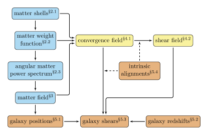
Figure 1: Flow chart of the typical simulation steps for a weak lensing galaxy survey. Superscripts indicate the section where a particular step is discussed in this work.

The outline of this work mirrors the steps for simulating a weak lensing galaxy survey, shown in Figure 1. In Section 2, we introduce the discretisation of the matter field into nested shells. In Section 3, we show how the matter field can be sampled iteratively using a transformed Gaussian distribution. In Section 4, we show how the weak lensing fields, which are integrals over all matter shells of lower redshift, can be computed iteratively via a recurrence. In Section 5, we show how we can populate the simulation with galaxies, as far as necessary for a cosmological galaxy survey. We then present an actual simulation using our models and implementation in Section 6. Finally, we discuss our results in Section 7. We provide some additional details of a more technical nature in Appendices A, B, and C.

2 Matter

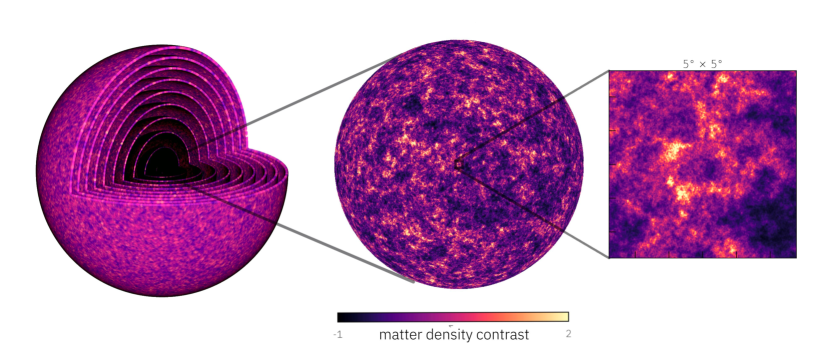
Figure 2: Ten shells of the discretised matter field as simulated by GLASS, with the first shell shown in detail. The simulations were created with $N_{\mathrm{side}}=8192$ ($8.05\times 10^{8}$ pixels) over a redshift range $0.0\leq z\leq 1.0$ in 10 shells of $\Delta z=0.1$. Shown are an illustration of the concentric nested matter shells at reduced resolution (left), a hemisphere of the innermost matter density shell at full resolution (centre), and a $5^{\circ}\times 5^{\circ}$ zoom into the first matter shell showing the details in the simulated fields (right).

Our overarching goal in this work is to simulate the universe as it is accessible to a wide-field galaxy survey. This is a universe at relatively late times, where radiation has become insignificant, and galaxies are formed. If there is dark energy, it does not imprint much of an interesting signal, except for an accelerated expansion of the cosmological background. A galaxy survey therefore ultimately probes matter, and particularly its spatial distribution, the so-called large-scale structure of the universe. But most matter appears to be dark matter, which we cannot detect directly. Instead, galaxy surveys actually observe two phenomena which trace the matter distribution, and which we must therefore ultimately simulate: weak gravitational lensing and the distribution of galaxies.

The way we approach the simulation mirrors the real astrophysical situation. First, we simulate the matter field itself. We do so by means of a statistical simulation, creating a random field with just the right spatial distribution to look like the large-scale structure of the universe, or at least when applying the statistics in which we are interested. Once we have the matter field, we then compute the associated effects of weak gravitational lensing and galaxies using a physically inspired model. We must hence be careful to get the matter distribution right to a high degree of precision and accuracy, even if we do not directly observe it, since everything else will depend on it later. We split the task in two: This section treats the definition of the matter fields in our simulation, while the next section discusses how to perform an accurate statistical simulation.

Throughout the text, we assume a standard $\Lambda$CDM cosmology. We expect that most results continue to hold in most extensions to $\Lambda$CDM, perhaps with some minor modification of e.g. the weak lensing sector.

Cosmological parameters and functions used here and in the following sections are the matter density fraction $\Omega_{\mathrm{m}}$, the Hubble function $H$, of which the present value is the Hubble constant $H_{0}$, and the dimensionless Hubble function $E=H/H_{0}$. Relevant distance functions are the comoving distance $d_{\mathrm{c}}$, and the transverse comoving distance $d_{\mathrm{M}}$. We mainly use dimensionless distance functions in units of the Hubble distance $d_{\mathrm{H}}=c/H_{0}$, namely the dimensionless comoving distance $x_{\mathrm{c}}=d_{\mathrm{c}}/d_{\mathrm{H}}$, and the dimensionless transverse comoving distance $x_{\mathrm{M}}=d_{\mathrm{M}}/d_{\mathrm{H}}$. The matter distribution in the universe is characterised by the matter density contrast $\delta=(\rho-\bar{\rho})/\bar{\rho}$, where $\rho$ is the matter density at a given point in space, and $\bar{\rho}$ is the cosmic mean matter density at that point in time.

Whenever results are computed explicitly, we must pick a specific set of background cosmological parameters values; we use $\Omega_{\mathrm{m}}=0.3$ and $H_{0}=70$ km s^-1 Mpc^-1.

2.1 Matter shells

To simulate the matter distribution of the universe, we must start by picking a suitable discretisation of three-dimensional space. Our goal is to simulate wide-field galaxy surveys for cosmology, and in particular those surveys that measure weak gravitational lensing. These surveys observe millions, and soon billions, of individual galaxies, by taking highly resolved images of galaxy fields. But they do not generally observe a significant amount of galaxies by any spectroscopic means. It follows that the kind of galaxy survey we wish to simulate has i) very high angular resolution, ii) fairly low resolution along the line of sight.

We construct our simulation accordingly, by dividing space into a series of nested spherical shells centred on the observer, as shown in Figure 2. The shells are specified by the redshifts

$$0=z_{0}<z_{1}<z_{2}<z_{3}<\ldots$$ (1)

of their boundaries, so that the shell with index $i>0$ contains redshifts $z$ with $z_{i-1}\leq z\leq z_{i}$. We can thus construct shells with any desired radial resolution. As we will show below, using nested shells also has another major advantage: Any outer shell can be simulated conditional only on its inner shells, so that we are able to iteratively construct an entire light cone, one shell at a time.

To compute the distribution of matter over a given shell $i$, we first fix a radial weight function $W_{i}$, which does not have to be normalised. We then use $W_{i}$ to project the matter density contrast $\delta$ in shell $i$ along the line of sight and onto the unit sphere. This yields a spherical function $\delta_{i}$ which is the averaged matter density contrast in shell $i$,

$$\delta_{i}(\hat{u})=\frac{\int\delta\bigl{(}d_{\mathrm{c}}(z)\,\hat{u}\bigr{)}\,W_{i}(z)\,\mathrm{d}z}{\int W_{i}(z)\,\mathrm{d}z}\;,$$ (2)

where $\hat{u}$ is a unit vector that parametrises the surface of the sphere, and the radial direction is parametrised as usual by the redshift $z$, so that $d_{\mathrm{c}}(z)\,\hat{u}$ is the three-dimensional comoving position of a point along the line-of-sight in the direction of $\hat{u}$.

In practice, we then need to further discretise $\delta_{i}$ in the angular dimensions, since we cannot compute with continuous functions on the sphere. We therefore construct a map $\delta_{i,k}=\delta_{i}(\hat{u}_{k})$ by evaluating the field $\delta_{i}$ over the spherical HEALPix grid of points $\hat{u}_{k}$, $k=1,\ldots,12\,N_{\mathrm{side}}^{2}$, with $N_{\mathrm{side}}$ a chosen HEALPix resolution parameter.

2.2 Matter weight functions

The radial weight function $W_{i}$ in the matter field (2) is in principle a free parameter of the simulation. In this work, we assume a uniform weight in redshift,

$$W_{i}(z)=\begin{cases}1&\text{if $z_{i-1}\leq z<z_{i}$,}\\ 0&\text{otherwise.}\end{cases}$$ (3)

We show in Sections 4 and 5 why the uniform weight function (3) is a good choice for simulations that include weak gravitational lensing or galaxy distributions.

Nevertheless, there are situations in which a different choice of matter weight function might be appropriate. For example, instead of (3), we could choose a uniform weight in comoving distance,

$$W_{i}(z)=\begin{cases}1/E(z)&\text{if $z_{i-1}\leq z<z_{i}$,}\\ 0&\text{otherwise,}\end{cases}$$ (4)

where $E$ is the dimensionless Hubble function. A true volume average of the matter density contrast is achieved if the weight function is proportional to the differential comoving volume,

$$W_{i}(z)=\begin{cases}x_{\mathrm{M}}^{2}(z)/E(z)&\text{if $z_{i-1}\leq z<z_{i}$,}\\ 0&\text{otherwise.}\end{cases}$$ (5)

Similarly, one can obtain maps of the true discretised mass by averaging the mean matter density,

$$W_{i}(z)=\begin{cases}\bar{\rho}(z)\,x_{\mathrm{M}}^{2}(z)/E(z)&\text{if $z_{i-1}\leq z<z_{i}$,}\\ 0&\text{otherwise.}\end{cases}$$ (6)

The weight functions (4), (5), and (6) may therefore be good choices in simulations where these physical quantities are of particular interest.

2.3 Angular matter power spectra

In principle, the discretised matter fields (2) can be provided from any suitable source. For example, it is possible to compute the matter density contrast $\delta_{i}$ in each shell from the outputs of an $N$-body simulation. Of course, we will normally want to generate the matter field as part of our simulation, and it must therefore contain the information that is relevant for cosmology. For the wide-field galaxy surveys we wish to simulate, that means we have to imprint the correct two-point statistics.

The two-point statistics of our generated matter fields are described by the angular matter power spectrum for each pair of shells. Many of the usual cosmology codes such as CAMB (Lewis et al., 2000; Lewis & Bridle, 2002), CCL (Chisari et al., 2019), or CLASS (Lesgourgues, 2011; Blas et al., 2011) can compute these spectra, which only requires the matter weight function ${W}_{i}$ that defines the matter field (2) in each shell $i$. Since $\delta_{i}$ is the projection of the matter field, and not the galaxy field, the angular matter power spectrum is computed without bias, redshift-space distortions, or any other such observational effect.

This is important, because the angular power spectra completely determine the underlying physical model for matter in the simulation. If the angular power spectra are computed e.g. using only the linear matter power spectrum, the simulation will only produce the linear matter field. Similarly, if the angular power spectra include a full non-linear treatment of matter, so will the simulation. The only task of the simulation is to reproduce the given angular power spectra faithfully, which we achieve using the methods of the next section.

The fact that we consider many relatively thin shells with a thickness of $\Delta z\lesssim 0.1$ in redshift means that the computation of the angular power spectra must largely be performed without use of Limber’s approximation (Limber, 1953; Kaiser, 1998; Simon, 2007). For this work, we use CAMB, since it is widely available, and allows Limber’s approximation to be switched off altogether. To work around a numerical issue in CAMB for flat matter weight functions that do not go to zero at $z=0$, we slightly modify (3) to increase linearly from zero at $z=0$ to unity at $z=0.1$, which is an otherwise negligible change. To obtain results at the required level of accuracy, we also set the TimeStepBoost parameter in CAMB to 5.

3 Sampling random fields on the sphere

The projected matter field of the previous section is at the heart of our simulations, as we will derive the weak gravitational lensing fields and the distribution of galaxies from the matter shells in the following sections. In this section, we show how we can produce random realisations of the projected matter density contrast (2) with

• a realistic distributions of values of the matter field, i.e. the one-point statistics, and

• the physically correct angular matter power spectrum, i.e. the two-point statistics.

These two criteria are imposed by our aim of producing simulations for the typical clustering and weak lensing studies done on wide-field galaxy surveys.

Sampling a Gaussian random map $X$ with fully specified statistical properties is readily done. However, the normal distribution is not a good model for the evolved matter fields that we wish to simulate. But if we apply a suitable transformation $f$ to the map, we obtain a second random map $Y=f(X)$ which now has a different distribution. By picking the right transformation, we will be able to recreate the one-point statistics of the matter field with high fidelity. The main challenge is then to imprint the correct two-point statistics onto the transformed map $Y$ via the transformation $f(X)$.

There is also a computational reason for basing our simulation on Gaussian random maps. The random realisations must contain the right correlations between the projected matter fields across all simulated shells. This means that we must either simulate, and hence hold in memory, all shells at once, or we must sample each new shell conditional on the existing shells. The former is usually not feasible for high-resolution maps without dedicated hardware. But the latter is particularly simple for Gaussian random maps.

3.1 Transformed Gaussian random fields

Let us for the moment assume that the transformation $f$ has already been fixed. Naturally, we must match the distribution of the Gaussian map $X$ to the desired distribution of the transformed map $Y$, such that the realisation has e.g. the correct mean and variance after the transformation. In the following, we always assume that the fields are homogeneous, i.e. invariant under rotations, as asserted by the cosmological principle. If the Gaussian map $X$ is homogeneous, it has the same mean $\mu$ and variance $\sigma^{2}$ everywhere, in the sense that for all points $\hat{u}$ on the sphere the expectation over realisations, denoted by $\langle\,\cdot\,\rangle$, is

$$\langle X(\hat{u})\rangle=\mu\quad\text{and}\quad\langle X^{2}(\hat{u})\rangle-\mu^{2}=\sigma^{2}\;.$$ (7)

Since $Y(\hat{u})=f\bigl{(}X(\hat{u})\bigr{)}$ and $X(\hat{u})$ is normally distributed with mean $\mu$ and variance $\sigma^{2}$, it follows that the transformation $Y=f(X)$ of a homogeneous Gaussian map $X$ remains homogeneous, and the distribution of $Y$, and thus all one-point statistics, depend solely on $f$, $\mu$, and $\sigma^{2}$. In particular, $Y$ has the same mean $\langle Y\rangle$ and variance $\langle Y^{2}\rangle-\langle Y\rangle^{2}$ everywhere.

Apart from the overall distribution of the values, the transformation must also imprint the realised map $Y$ with the correct two-point statistics, since that is where we extract cosmological information from the simulations. If $Y$ and $Y^{\prime}$ are two not necessarily distinct homogeneous spherical random fields, the correlation in the respective points $\hat{u}$ and $\hat{u}^{\prime}$ is described by the angular correlation function $C$,

$$\langle Y(\hat{u})\,Y^{\prime}(\hat{u}^{\prime})\rangle=C(\theta)\;,$$ (8)

which, due to homogeneity, is a function of the angle $\theta$ between $\hat{u}$ and $\hat{u}^{\prime}$ alone. Let both fields be the respective transformations $Y=f(X)$ and $Y^{\prime}=f^{\prime}(X^{\prime})$ of homogeneous Gaussian fields $X$ and $X^{\prime}$, so that $X(\hat{u})$ and $X^{\prime}(\hat{u}^{\prime})$ are jointly normal with the respective means $\mu$ and $\mu^{\prime}$ and variances $\sigma^{2}$ and $\sigma^{\prime 2}$. If the correlations between $X$ and $X^{\prime}$ are given by the correlation function $G$,

$$\langle X(\hat{u})\,X^{\prime}(\hat{u}^{\prime})\rangle=G(\theta)\;,$$ (9)

the joint distribution of $X(\hat{u})$ and $X^{\prime}(\hat{u}^{\prime})$, being jointly normal random variables, is completely described by the values of $\mu$, $\mu^{\prime}$, $\sigma^{2}$, $\sigma^{\prime 2}$, and $G(\theta)$. It follows that the correlation (8) between the transformed random variables $Y(\hat{u})=f(X(\hat{u}))$ and $Y^{\prime}(\hat{u}^{\prime})=f^{\prime}(X(\hat{u}^{\prime}))$ must be a function of these variables alone,

$$C(\theta)=C\bigl{(}G(\theta);\mu,\mu^{\prime},\sigma^{2},\sigma^{\prime 2}\bigr{)}\;,$$ (10)

where the form of this function depends on the transformations $f$ and $f^{\prime}$ between the fields. The function $C$ will normally be obtained by computing (8) explicitly. Inverting the result, either analytically or numerically, then yields the function

$$G(\theta)=G\bigl{(}C(\theta);\mu,\mu^{\prime},\sigma^{2},\sigma^{\prime 2}\bigr{)}\;,$$ (11)

which characterises the two-point statistics of the Gaussian maps in terms of the two-point statistics of their transformations.

Given a transformation $f$, we can hence expect to also be given the relations (10) and (11) for translating the desired correlations $C(\theta)$ of $Y$ into the correlations $G(\theta)$ to be imprinted onto the Gaussian random field $X$.

3.2 Lognormal fields

One popular choice of transformation $f$ for matter fields is the lognormal distribution (e.g. Coles & Jones, 1991; Kayo et al., 2001; Hilbert et al., 2011; Xavier et al., 2016),

$$f(x)=\lambda\,(\mathrm{e}^{x}-1)\;,$$ (12)

where the parameter $\lambda$ is the so-called “shift” of the lognormal distribution. Since the exponential is limited to positive values, the value of $\lambda$ is effectively the lower bound of variates of the distribution. A volume devoid of any matter has matter density contrast $\delta=-1$, so a shift parameter $\lambda=1$ is usually assumed for matter fields.

The simulation of lognormal random fields on the sphere was discussed in detail by Xavier et al. (2016), and we only repeat the relations (10) and (11) here,

$$C(\theta) =\alpha\alpha^{\prime}\Bigl{\{}\mathrm{e}^{G(\theta)}-1\Bigr{\}}\;,$$ (13)

$$G(\theta) =\ln\Bigl{\{}1+\frac{C(\theta)}{\alpha\alpha^{\prime}}\Bigr{\}}\;,$$ (14)

which are characterised by the parameter $\alpha=\langle Y\rangle+\lambda$ for $Y$, and similarly $\alpha^{\prime}$ for $Y^{\prime}$.

Lognormal distributions are widely used not only for simulating the matter field (Coles & Jones, 1991; Böhm et al., 2017; Abramo et al., 2016; Abramo et al., 2022) but also weak lensing convergence fields (Hilbert et al., 2011; Clerkin et al., 2017; Giocoli et al., 2017; Gatti et al., 2020). In particular, Hall & Taylor (2022) showed that lognormal distributions reproduce, up to reasonable precision and accuracy, the bispectrum (i.e. three-point statistics) and the covariance (i.e. four-point statistics) of the underlying fields when compared to results obtained from $N$-body simulations over the typical scales for a Stage 4 photometric galaxy survey. However, the agreement between lognormal and $N$-body simulations for higher-order statistics is not perfect, and it is conditional on the scales and configurations analysed (Piras et al., 2023).

3.3 Gaussian angular power spectra

Having obtained a suitable transformation $f$, such as e.g. the lognormal transformation (12), and derived its relations (10) and (11) for the two-point statistics, we face two further issues before we can actually sample the Gaussian random map $X$: Firstly, theoretical calculations usually do not produce $C(\theta)$, but instead the angular matter power spectrum $C_{l}$ for the matter fields (2). And secondly, the procedure for sampling a Gaussian random map also requires the Gaussian angular power spectrum $G_{l}$ instead of $G(\theta)$. We must therefore convert between the angular correlation functions and angular power spectra.

The conversion is done using the well-known transforms between angular correlation functions and angular power spectra,

$$C(\theta)=\sum_{l=0}^{\infty}\frac{2l+1}{4\pi}\,C_{l}\,P_{l}(\cos\theta)\;,$$ (15)

with $P_{l}$ the Legendre polynomial of degree $l$, and

$$C_{l}=2\pi\int_{0}^{\pi}\!C(\theta)\,P_{l}(\cos\theta)\sin(\theta)\,\mathrm{d}\theta\;,$$ (16)

and similarly for $G(\theta)$ and $G_{l}$. In theory, the steps to obtain $G_{l}$ from $C_{l}$ are hence straightforward:

• Compute the correlations $C(\theta)$ from $C_{l}$ using (15),

• apply relation (11) to obtain $G(\theta)$ from $C(\theta)$, and

• compute $G_{l}$ from from $G(\theta)$ using (16).

Overall, the computation can be summarised as

$$C_{l}\to C(\theta)\to G(\theta)\to G_{l}\;,$$ (17)

which we call the “backward” sequence. This name is owed to the fact that the sampling of a Gaussian random field from $G_{l}$ and subsequent transformation $Y=f(X)$ instead correspond to

$$G_{l}\to G(\theta)\to C(\theta)\to C_{l}\;,$$ (18)

which we consequently call the “forward” sequence.

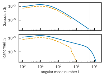
Figure 3: The effect of a band limit in the Gaussian angular power spectrum $G_{l}$ on the transformed angular power spectrum $C_{l}$, here for the lognormal transformation of two inputs (solid, dashed) with different band limits (vertical lines). The shape of $C_{l}$ depends critically on the band limit of $G_{l}$, and will generally have a higher band limit.

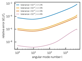
Figure 4: Relative error $\Delta C_{l}/C_{l}$ of the realised angular power spectra using the Gauss–Newton solver. Shown are various settings of the nominal tolerance of the algorithm and the length $n$ of the internal Legendre transforms relative to the length $N$ of the inputs.

In practice, we can usually neither evaluate the infinite sum in (15) for all $\theta$, nor the continuous integral in (16) for all $l$, and we always have to work with angular power spectra of finite length. But imposing a band limit on both $C_{l}$ and $G_{l}$ is problematic: Xavier et al. (2016) noted that, for lognormal fields, a band-limited $G_{l}$ yields values $C_{l}$ beyond the band limit, and the same holds more generally for any non-linear transformation $f$. The effect is shown in Figure 3.

To work around the finite nature of their transforms, the approach of Xavier et al. (2016) was to take a given band-limited $C_{l}$ and compute $G_{l}$ using the backward sequence (17) at a higher band limit. This is shown to achieve per-cent level fidelity of the realisation when the band limit is set very generously, which is computationally expensive, since the cost of a discrete spherical harmonic transform increases with the square of the band limit. It also requires regularisation of the transformed angular power spectra, which may at least partly be due to the fact that $C_{l}$ contains zeros when padded to a higher band limit, rendering the conversion between $G_{l}$ and $C_{l}$ ill-defined.

On closer inspection, the difficulty arises from use of the backward sequence (17) for directly computing $G_{l}$ from a given band-limited $C_{l}$. But there are other ways to approach the conversion (Shields et al., 2011). For example, we can try and solve the inverse problem instead, which is: find a band-limited Gaussian angular power spectrum $G_{l}$ of length $N$ such that the forward sequence (18) recovers $N$ given values $C_{l}$. As it turns out, that approach is both simpler and more accurate. All it needs is a standard numerical method for the solution, or approximate solution, of non-linear equations. Here, we use the Gauss–Newton algorithm.

To start, let $G_{l}$ be an initial guess for the Gaussian angular power spectrum, and let $F_{l}$ be the residuals of the forward sequence (18) and given values $C_{l}$. The Gauss–Newton update moves from $G_{l}$ to $G_{l}+S_{l}$, where the step $S_{l}$ is found by solving the matrix equation

$$\sum_{l^{\prime}}\frac{\partial F_{l}}{\partial G_{l^{\prime}}}\,S_{l^{\prime}}=-F_{l}\;.$$ (19)

Applying the derivative to the forward sequence (18) yields

$$\frac{\partial F_{l}}{\partial G_{l^{\prime}}}=2\pi\int_{0}^{\pi}\!\frac{\partial C(\theta)}{\partial G(\theta)}\,\frac{\partial G(\theta)}{\partial G_{l^{\prime}}}\,P_{l}(\cos\theta)\sin(\theta)\,\mathrm{d}\theta\;.$$ (20)

Note that $\partial C(\theta)/\partial G(\theta)$ is the derivative of (10) with respect to $G(\theta)$; for short, let $\partial C(\theta)/\partial G(\theta)=\dot{C}(\theta)$. Like $C(\theta)$ itself, the function $\dot{C}$ is characteristic of the transformation $f$, and can be computed. The other derivative in (20) is readily found using (15),

$$\frac{\partial G(\theta)}{\partial G_{l^{\prime}}}=\frac{2l^{\prime}+1}{4\pi}\,P_{l^{\prime}}(\cos\theta)\;.$$ (21)

Using (20) and (21), the matrix equation (19) becomes the integral

$$2\pi\int_{0}^{\pi}\!\dot{C}(\theta)\,S(\theta)\,P_{l}(\cos\theta)\sin(\theta)\,\mathrm{d}\theta=-F_{l}\;,$$ (22)

where we have exchanged summation and integration to transform $S_{l}$ into $S(\theta)$ using (15),

$$\sum_{l^{\prime}}\frac{2l^{\prime}+1}{4\pi}\,S_{l^{\prime}}\,P_{l^{\prime}}(\cos\theta)=S(\theta)\;.$$ (23)

Since the resulting equation (22) itself is precisely the transform (16), we obtain the result that the Gauss–Newton step must obey $\dot{C}(\theta)\,S(\theta)=-F(\theta)$ in real space. The solution of (19) therefore has the representation

$$S(\theta)=-\frac{F(\theta)}{\dot{C}(\theta)}\;,$$ (24)

which can be transformed back into $S_{l}$ using (16). It only remains to find an initial guess for the values $G_{l}$, which we do using the backward sequence (17) for the fixed length $N$. This generally yields a starting point such that the Gauss–Newton algorithm converges in just a handful of iterations.

Solving for a Gaussian angular power spectrum $G_{l}$ with the above method still involves the transforms (15) and (16), so that the true, continuous transforms must in practice still be approximated by finite, discrete ones. The crucial difference is that we do not transform $C$ and $G$ here, but instead $F$ and $S$. Depending on the desired accuracy, we can choose an arbitrarily large length $n\gg N$ for the transforms; since they are internal to the Gauss–Newton step, both $C_{l}$ and $G_{l}$ remain of the length $N$ that we ultimately want to realise. As mentioned earlier, this quadratically improves the sampling performance over methods relying on padded spectra.

In practical terms, we note that the transforms (15) and (16) are effectively discrete Legendre expansions with slightly modified coefficients. We can compute them using the method we describe in Appendix A, which maps $n$ values $F_{l}$ to $n$ values $F(\theta)$ over a regular grid of $\theta$ values using the Fast Fourier Transform. The mapping is one-to-one and invertible, so that we can transform back and forth without loss of information. Commonly used methods based on Gaussian quadrature, as well as the method of Driscoll & Healy (1994), or the method of Healy et al. (2003) used by Xavier et al. (2016), map between $n$ values of $F_{l}$ and $2n$ values of $F(\theta)$, and are therefore clearly not generally invertible. Our transforms are very fast and do not construct any large matrices, so that values of e.g. $n>100\,000$ are readily achievable.

To give an idea of the accuracy of our new method for computing Gaussian angular power spectra, Figure 4 shows the relative error of the lognormal transformation of a typical angular power spectrum $C_{l}$ with $l\leq 5\,000$, i.e. $N=5\,001$. We show the solution of the Gaussian angular power spectrum $G_{l}$ using a number of settings for the nominal tolerance of the Gauss–Newton algorithm, as well as different lengths $n$ of the internal Legendre transforms. To compare the result to the input, we compute the forward sequence (18) for each solution $G_{l}$ using $1\,000\,000$ terms in the Legendre expansion. We find that, in the regime shown, the accuracy of the solution depends mainly on $n$. We adopt a tolerance of $10^{-5}$ and $n=3N$ as good default values, having a relative error better than $10^{-4}$ everywhere, with the understanding that better accuracy is readily available.

Overall, this new method allows us to simulate transformed Gaussian random fields on the sphere in such a way that the first $N$ modes of the angular power spectrum match any given values $C_{l}$ reliably. In principle, we could therefore accurately simulate maps of the matter fields up to the band limit $l_{\max}$ of a HEALPix map, which for a given resolution parameter $N_{\mathrm{side}}$ is $l_{\max}=3N_{\mathrm{side}}-1$. However, as shown in Figure 3, the transformed random field will in general not be band-limited to $l_{\max}$. Even if the angular power spectrum is simulated accurately up to $l_{\max}$, it is hence difficult to actually use this part of the spectrum for practical purposes, due to aliasing from modes beyond the band limit. To obtain interpretable results, we find values of $N$ somewhere between $N_{\mathrm{side}}$ and $2N_{\mathrm{side}}$ most reliable.

Because they are generally useful beyond this specific work, we provide our implementations of the transforms (15) and (16) as the stand-alone transformcl package for Python, and our solver for Gaussian angular power spectra as the stand-alone gaussiancl package for Python.

3.4 Zero monopoles

Computer codes often produce theoretical angular matter power spectra with a vanishing monopole. For the simulated matter shells, this is problematic for two reasons: Physically, it is not the case that a matter shell of finite size has an exactly vanishing average density contrast with no variance at all. And mathematically, a vanishing monopole results in an ill-defined Gaussian transformation. The first issue requires better theoretical computations, which is not part of our work. But we can try and mitigate the second issue ourselves.

More specifically, the problem is that a vanishing monopole value $C_{0}=0$ in the transformed angular power spectrum will generally result in a negative monopole $G_{0}$ in the Gaussian angular power spectrum. This occurs because the transformation mixes Gaussian modes with non-zero random values from beyond the monopole into the monopole of the transformed field. To counteract the randomness, at least formally, a negative variance is required, and the Gaussian random field becomes ill-defined.

To work around this issue, we can exclude both monopoles $C_{0}$ and $G_{0}$ from our solver, fixing $G_{0}=0$. After the transformation, the realised field will have a value $C_{0}>0$ that is realistic, but arbitrary. The result is essentially a smooth extrapolation to $l=0$ of the given modes $C_{l}$ with $l>0$, which is the best we can do to obtain a well-defined random field.

The Gauss–Newton solver is readily adapted to ignore $C_{0}$ and fix $G_{0}$ to its initial value: The latter is equivalent to $S_{0}$ in the update step (24) being zero, and there always exists a value of $C_{0}$ such that this is the case. Since the given $C_{0}$ is ignored, we can arbitrarily assume that it was that particular value. To obtain the constrained solution, it therefore suffices to set $S_{0}=0$ and $F_{0}=0$ in the unconstrained solution.

3.5 Sampling the Gaussian random fields

To sample a Gaussian random field $X$ on the sphere with a given angular power spectrum $G_{l}$, we sample the complex-valued modes $a_{lm}$ of its spherical harmonic expansion,

$$X(\hat{u})=\sum_{lm}a_{lm}\,Y_{lm}(\hat{u})\;.$$ (25)

We can obtain a number of conditions on the distribution of the $a_{lm}$. If the field is homogeneous, i.e. invariant under rotations, the mean of the modes with $l>0$ must vanish,

$$\langle a_{lm}\rangle=0\;.$$ (26)

If the field also has zero expectation, as is the case for the matter density contrast, the same holds for the monopole $l=0$. The angular power spectrum determines the covariance of the modes with numbers $l,m$ and $l^{\prime},m^{\prime}$,

$$\langle a_{lm}\,a_{l^{\prime}m^{\prime}}^{*}\rangle=\delta^{\mathrm{K}}_{ll^{\prime}}\,\delta^{\mathrm{K}}_{mm^{\prime}}\,G_{l}\;,$$ (27)

where the Kronecker delta expresses that differently-numbered modes are uncorrelated, which follows from homogeneity of the field. For a real-valued field, the symmetry $a_{lm}^{*}=(-1)^{m}\,a_{l,-m}$ and the covariance (27) together imply that the pseudo-variance of the modes vanishes for $m\neq 0$,

$$\langle a_{lm}^{2}\rangle=(-1)^{m}\,\langle a_{lm}\,a_{l-m}^{*}\rangle=\delta^{\mathrm{K}}_{m0}\,G_{l}\;.$$ (28)

Finally, since any linear combination of normal random variables remains normally distributed, we can sample the modes $a_{lm}$ themselves as complex normal random variables.

The sampling is most easily done by splitting each $a_{lm}$ into its real and imaginary part,

$$a_{lm}=x_{lm}+\mathrm{i}\,y_{lm}\;,$$ (29)

and sampling the set of $x_{lm}$ and $y_{lm}$ as a real-valued multivariate normal random variable. If the field is real-valued, the symmetry $a_{lm}^{*}=(-1)^{m}\,a_{l,-m}$ implies that only the $x_{lm}$ and $y_{lm}$ with $m\geq 0$ need to be sampled. By condition (26), the means of all $x_{lm}$ and $y_{lm}$ vanish,

$$\langle x_{lm}\rangle=\langle y_{lm}\rangle=0\;.$$ (30)

By conditions (27) and (28), a pair of $x_{lm}$ and $y_{lm}$ with $m>0$ is uncorrelated, $\langle x_{lm}\,y_{lm}\rangle=0$, with equal variance,

$$\langle x_{lm}^{2}\rangle=\langle y_{lm}^{2}\rangle=\frac{G_{l}}{2}\qquad(m>0)\;.$$ (31)

For $m=0$, the same conditions imply that

$$\langle x_{l0}^{2}\rangle=G_{l}\quad\text{and}\quad\langle y_{l0}^{2}\rangle=0\;,$$ (32)

and thus $y_{l0}=0$ identically. Furthermore, by condition (27), the $x_{lm}$ and $y_{lm}$ are pairwise uncorrelated for different modes. We therefore only have to sample for $m\geq 0$ each pair of $x_{lm}$ and $y_{lm}$ independently, with zero mean and the correct variance. After an inverse spherical harmonic transform, we obtain the Gaussian random field $X$ with the prescribed statistics.

When correlated Gaussian random fields $X^{i}$ and $X^{j}$ are simulated, with $i$ and $j$ some indices, there is an additional condition that the covariance of their respective modes $a_{lm}^{i}$ and $a_{lm}^{j}$ recovers the angular cross-power spectrum $G_{l}^{ij}$,

$$\langle a_{lm}^{i}\,a_{l^{\prime}m^{\prime}}^{j*}\rangle=\delta^{\mathrm{K}}_{ll^{\prime}}\,\delta^{\mathrm{K}}_{mm^{\prime}}\,G_{l}^{ij}\;.$$ (33)

For fixed values of $l$ and $m$, the sets $\bm{x}_{lm}=\{x_{lm}^{1},x_{lm}^{2},\ldots\}$ and $\bm{y}_{lm}=\{y_{lm}^{1},y_{lm}^{2},\ldots\}$ taken over different fields are thus multivariate normal random vectors with covariance matrix

$$\langle x_{lm}^{i}\,x_{lm}^{j}\rangle=\langle y_{lm}^{i}\,y_{lm}^{j}\rangle=\frac{G_{l}^{ij}}{2}\;,\quad m>0\;,$$ (34)

$$\langle x_{l0}^{i}\,x_{l0}^{j}\rangle=G_{l}^{ij}\quad\text{and}\quad\langle y_{l0}^{i}\,y_{l0}^{j}\rangle=0\;,$$ (35)

and remain independent across different modes. For $n$ correlated Gaussian random fields, we thus have to sample the multivariate normal random variables $\bm{x}_{lm}$ and $\bm{y}_{lm}$ for each $l,m$ independently from their $n\times n$ covariance matrix.

For our specific application, this is problematic. At the highest map resolutions, it is not feasible to sample the integrated matter fields for hundreds of shells all at once, due to the amount of memory required. However, it is possible to sample multivariate normal random variables iteratively, which in our case means: shell by shell. The technique, shown in Appendix B, allows us to generate each new integrated matter field in turn, while still imprinting the correct correlations with previous shells. In addition, we use that the correlations of the matter field along the line of sight become negligible above a certain correlation length, of the order of 100 Mpc. As we show in the appendix, the iterative sampling then only requires us to store those fields which are effectively still correlated, so that we are able to sample arbitrarily many shells without increasing our memory requirements. Only the thickness of the shells determines the amount of correlation between them, and thus how many previous shells we must store. We show how an informed choice can be made in Section 6.

4 Weak gravitational lensing

We now use our realisation of the matter fields in each shell to compute other, related fields, namely the convergence and shear of weak gravitational lensing. The fact that we compute lensing from matter in deterministic fashion, close to the real physical situation, means that we do not have to make any additional assumptions about e.g. the statistical distributions of the fields.

On the other hand, it also means we have to overcome two associated difficulties: First and foremost, the fact that we wish to continue sampling the fields iteratively, shell by shell. Lensing happens continuously between source and observer, and the computation of the lensing fields requires an integral over the line of sight. We therefore have to develop a way to perform the computation iteratively. The second difficulty is also related to the integration: the matter fields that we sample are already discretised into shells, and we have to approximate the lensing integral using the existing discretisation.

4.1 Convergence

We compute the convergence field $\kappa$ from the matter density contrast $\delta$ in the Born approximation, i.e. along an undeflected line of sight. In the case of weak lensing, this approximation is sufficient even for upcoming weak lensing surveys (Petri et al., 2017). The convergence for a source located at angular position $\hat{u}$ and redshift $z$ is hence (see e.g. Schneider et al., 2006)

$$\kappa(\hat{u};z)\\ =\tfrac{3\Omega_{m}}{2}\int_{0}^{z}\!\delta\bigl{(}d_{\mathrm{c}}(z^{\prime})\,\hat{u}\bigr{)}\,\tfrac{x_{\mathrm{M}}(z^{\prime})\,x_{\mathrm{M}}(z^{\prime},z)}{x_{\mathrm{M}}(z)}\,\tfrac{1+z^{\prime}}{E(z^{\prime})}\,\mathrm{d}z^{\prime}\;,$$ (36)

where we have used the dimensionless distance and Hubble functions. The integral in (36) presents two immediate problems for our computations: Firstly, we do not have access to the continuous matter distribution $\delta$, but only the discretised matter fields $\delta_{i}$ in each shell. And secondly, the integral in (36) depends on all matter below the source redshift $z$, while we want to perform the computation iteratively, keeping only a limited number of matter fields in memory.

To solve these problems, we impose three additional requirements for the matter shells $i=0,1,\ldots$ and their matter weight functions $W_{i}$. The first requirement is that every shell $i$ has an associated effective redshift $\bar{z}_{i}$ which is, in some sense, representative of the shell. For example, this could be the mean redshift of the matter weight function,

$$\bar{z}_{i}=\frac{\int z\,W_{i}(z)\,\mathrm{d}z}{\int W_{i}(z)\,\mathrm{d}z}\;,$$ (37)

but other reasonable choices exist. The second requirement is that the matter weight functions of shells $j<i$ vanish beyond the effective redshift $\bar{z}_{i}$,

$$W_{j}(z)=0\qquad\text{($j<i$ and $z\geq\bar{z}_{i}$)}\;.$$ (38)

The third requirement is that the matter weight functions of shells $j>i$ vanish below the effective redshift $\bar{z}_{i}$,

$$W_{j}(z)=0\qquad\text{($j>i$ and $z\leq\bar{z}_{i}$)}\;.$$ (39)

In short, the requirements say that each matter shell has a representative redshift which partitions the matter weight functions of all other shells. This is clearly the case for the effective redshifts (37) and the matter weight function (3).

To then approximate the continuous integral (36) by a discrete sum, we first have to bring the integrand into a shape that matches the definition (2) of the integrated matter fields. Using the trivial partition of unity

$$\sum_{j}\frac{W_{j}(z)}{\sum_{k}W_{k}(z)}=1\;,$$ (40)

where the sums extend over all shells, we can introduce the matter weight function $W_{i}$ into the convergence (36),

$$\kappa(\hat{u};z)\\ =\tfrac{3\Omega_{m}}{2}\sum_{j}\int_{0}^{z}\!\delta\bigl{(}d_{\mathrm{c}}(z^{\prime})\,\hat{u}\bigr{)}\,W_{j}(z^{\prime})\,q(z^{\prime};z)\,\mathrm{d}z^{\prime}\;,$$ (41)

with the function $q$ being short for the geometric and weight factors,

$$q(z^{\prime};z)=\frac{1}{\sum_{k}W_{k}(z^{\prime})}\,\frac{x_{\mathrm{M}}(z^{\prime})\,x_{\mathrm{M}}(z^{\prime},z)}{x_{\mathrm{M}}(z)}\,\frac{1+z^{\prime}}{E(z^{\prime})}\;.$$ (42)

To make our approximation, we now assume that the weight function $W_{j}$ in the integral (41) is so localised that the function $q$ is constant and equal to its value at the effective redshift $\bar{z}_{j}$ for shell $j$,

$$\kappa(\hat{u};z)\\ \approx\tfrac{3\Omega_{m}}{2}\sum_{j}q(\bar{z}_{j};z)\int_{0}^{z}\!\delta\bigl{(}d_{\mathrm{c}}(z^{\prime})\,\hat{u}\bigr{)}\,W_{j}(z^{\prime})\,\mathrm{d}z^{\prime}\;.$$ (43)

If the support of $W_{j}$ corresponds to a thin shell, this holds for $z>\bar{z}_{j}$ as long the sum of weights in (42) changes as slowly as the cosmological quantities. We can then evaluate the convergence (43) in the effective redshift $\bar{z}_{i}$ for a given shell $i$: By requirement (38), we can truncate the sum before shell $i$, since $q(\bar{z}_{i};\bar{z}_{i})=0$ by definition,

$$\kappa_{i}(\hat{u})=\kappa(\hat{u};\bar{z}_{i})\\ =\tfrac{3\Omega_{m}}{2}\sum_{j=0}^{i-1}q(\bar{z}_{j};\bar{z}_{i})\int_{0}^{\bar{z}_{i}}\!\delta\bigl{(}d_{\mathrm{c}}(z^{\prime})\,\hat{u}\bigr{)}\,W_{j}(z^{\prime})\,\mathrm{d}z^{\prime}\;,$$ (44)

and by requirement (39), we can extend the remaining integrals over all redshifts. If we compare the resulting expression and the integrated matter fields (2), we find that we can indeed write a discrete approximation of the convergence,

$$\kappa_{i}(\hat{u})=\tfrac{3\Omega_{m}}{2}\sum_{j=0}^{i-1}\tfrac{x_{\mathrm{M}}(\bar{z}_{j})\,x_{\mathrm{M}}(\bar{z}_{j},\bar{z}_{i})}{x_{\mathrm{M}}(\bar{z}_{i})}\,\tfrac{1+\bar{z}_{j}}{E(\bar{z}_{j})}\,w_{j}\,\delta_{j}(\hat{u})\;,$$ (45)

where we have defined the lensing weights $w_{j}$ to contain the dependency on the matter weight functions,

$$w_{j}=\frac{1}{W_{j}(\bar{z}_{j})}\int W_{j}(z)\,\mathrm{d}z\;.$$ (46)

The approximation (45) as such is well known: Lensing can be approximated by collapsing a continuous matter distribution onto a set of discrete lensing planes. Our main insight here is the exact form of the lensing weights (46) for the given matter weight functions, as well as the requirements (38) and (39) on them.

Although the convergence (45) is now discretised, it still cannot be computed iteratively, since the geometric factor in each term depends explicitly on the shells $i$ and $j$. Here, the distance ratio relation of Schneider (2016) is a powerful tool: For $i\geq 2$, define the ratio of distance ratios

$$t_{i}=\frac{x_{\mathrm{M}}(\bar{z}_{i-2},\bar{z}_{i})}{x_{\mathrm{M}}(\bar{z}_{i})}\bigg{/}\frac{x_{\mathrm{M}}(\bar{z}_{i-2},\bar{z}_{i-1})}{x_{\mathrm{M}}(\bar{z}_{i-1})}\;.$$ (47)

The distance ratios for any other redshift $\bar{z}_{j}$ then obey

$$\frac{x_{\mathrm{M}}(\bar{z}_{j},\bar{z}_{i})}{x_{\mathrm{M}}(\bar{z}_{i})}=t_{i}\,\tfrac{x_{\mathrm{M}}(\bar{z}_{j},\bar{z}_{i-1})}{x_{\mathrm{M}}(\bar{z}_{i-1})}+(1-t_{i})\,\tfrac{x_{\mathrm{M}}(\bar{z}_{j},\bar{z}_{i-2})}{x_{\mathrm{M}}(\bar{z}_{i-2})}\;.$$ (48)

As shown by Schneider (2016), this relation is exact and a consequence of the mathematical form of the transverse comoving distance in generic Robertson-Walker space-times. Inserting (48) into the discrete approximation (45), we immediately obtain a recurrence relation for the convergence,

$$\kappa_{i}(\hat{u})=t_{i}\,\kappa_{i-1}(\hat{u})+(1-t_{i})\,\kappa_{i-2}(\hat{u})\\ +\tfrac{3\Omega_{m}}{2}\,\tfrac{x_{\mathrm{M}}(\bar{z}_{i-1})\,x_{\mathrm{M}}(\bar{z}_{i-1},\bar{z}_{i})}{x_{\mathrm{M}}(\bar{z}_{i})}\,\tfrac{1+\bar{z}_{i-1}}{E(\bar{z}_{i-1})}\,w_{i-1}\,\delta_{i-1}(\hat{u})\;.$$ (49)

This is equivalent to the multi-plane formalism for the deflection in strong gravitational lensing (Petkova et al., 2014; Schneider, 2019).

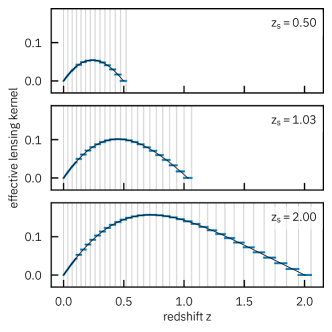
Figure 5: Effective lensing kernel of the lensing recurrence for source redshifts $z_{\mathrm{s}}=0.50$ (top), $z_{\mathrm{s}}=1.03$ (middle), and $z_{\mathrm{s}}=2.00$ (bottom). Vertical lines indicate the boundaries of matter shells with constant thickness in comoving distance $\Delta d_{\mathrm{c}}=150$ Mpc. Also shown is the true lensing kernel (black).

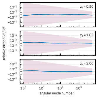
Figure 6: The relative error in the angular power spectra for the effective lensing kernels of the lensing recurrence, as shown in Figure 5. The shaded area shows the standard deviation of a Gaussian field for comparison. Here and below, the logarithmic $y$-axis changes to linear when passing through the origin.

Overall, we have obtained the lensing recurrence (49) by making specific choices for our matter weight functions, and one single approximation in (43). To test this approximation, we can compare the effective lensing kernel of the recurrence, i.e. the resulting factor in (36) multiplying $\delta$, to the true lensing kernel. This is done in Figure 5 for source redshifts $z_{\mathrm{s}}=0.50$, $z_{\mathrm{s}}=1.03$, and $z_{\mathrm{s}}=2.00$. For the matter shells, we use a constant size of $\Delta d_{\mathrm{c}}=150$ Mpc in comoving distance, which is a reasonable choice, as we show in Section 6. The effective lensing kernel of our approximation is essentially the matter weight function in each shell, scaled by the lensing recurrence, so that the flat matter weight function (3) is a good global approximation to the true kernel. As one would expect, thinner shells result in a better approximation, since we are essentially computing the convergence integral (36) as a Riemann sum. For the same reason, the approximation improves naturally with higher source redshifts, which cover a larger number of shells.

For a more quantitative check, we can compute the angular power spectra of the effective lensing kernels, and compare the results to the true angular convergence power spectra for each source redshift. We compute the true spectra with CAMB, for angular modes up to number $l=5\,000$, without Limber’s approximation. Figure 6 shows the resulting relative errors. For shells with $\Delta d_{\mathrm{c}}=150$ Mpc, the error is well below the per cent level, and much smaller than the expected uncertainty due to cosmic variance, which we approximate here by the Gaussian one for the sake of simplicity.

4.2 Shear

Having found the convergence (36) for weak lensing by our simulated matter distribution, we can obtain other weak lensing fields by applying the spin-raising and spin-lowering operators $\eth$ and $\bar{\eth}$ (see e.g. Boyle, 2016). Their effect on the spin-weighted spherical harmonics ${}_{s}Y_{lm}$ is

$$\eth\,{}_{s}Y_{lm} =+\sqrt{(l-s)(l+s+1)}\,{}_{s+1}Y_{lm}\;,$$ (50)

$$\bar{\eth}\,{}_{s}Y_{lm} =-\sqrt{(l+s)(l-s+1)}\,{}_{s-1}Y_{lm}\;,$$ (51)

where the spin-$0$ spherical harmonic ${}_{0}Y_{lm}$ is the scalar spherical harmonic $Y_{lm}$.

On the sphere, the Poisson equation for weak lensing reads

$$2\kappa=\eth\bar{\eth}\psi\;,$$ (52)

and relates the convergence $\kappa$ to the lensing (or deflection) potential $\psi$. Let $\kappa_{lm}$ be the modes of the spherical harmonic expansion of the convergence field,

$$\kappa(\hat{u})=\sum_{lm}\kappa_{lm}\,Y_{lm}(\hat{u})\;,$$ (53)

and similarly $\psi_{lm}$ for the lensing potential $\psi$. Inserting the expansions into (52) and applying the operators (50) and (51), the Poisson equation in harmonic space reduces to a simple algebraic relation between the modes $\kappa_{lm}$ and $\psi_{lm}$,

$$2\kappa_{lm}=-l\,(l+1)\,\psi_{lm}\;.$$ (54)

We can readily solve for $\psi_{lm}$, except when $l=m=0$. The mode $\psi_{00}$, however, describes a constant offset of the potential without physical meaning, and can be given an arbitrary value. We can thus completely determine the lensing potential from the convergence via the spherical harmonic expansion.

The principal observational effect of weak gravitational lensing, discussed below in Section 5, is caused by the shear field, commonly denoted $\gamma$. Shear is the spin-$2$ field obtained by applying $\eth$ twice to the lensing potential,

$$2\gamma=\eth\eth\psi\;.$$ (55)

As before, we can obtain an algebraic relation between the modes $\gamma_{lm}$ of the shear field and $\psi_{lm}$,

$$2\gamma_{lm}=\sqrt{(l+2)\,(l+1)\,l\,(l-1)}\,\psi_{lm}\;.$$ (56)

An alternative definition is sometimes used where the shear is a spin-$(-2)$ field $\gamma=\bar{\eth}\bar{\eth}\psi$. However, this yields exactly the same modes (56). The difference between the definitions is whether the coordinate system is left- or right-handed, and the shear in one definition is the complex conjugate of the shear in the other.

From (56), it follows that the shear modes with $l<2$ vanish identically, as expected for a spin-$2$ field. We can hence treat the case $\gamma_{00}=0$ separately, and compute the remaining shear modes with $l>0$ directly from the convergence modes by combining (56) and (54),

$$\gamma_{lm}=-\sqrt{\frac{(l+2)\,(l-1)}{l\,(l+1)}}\,\kappa_{lm}\;.$$ (57)

While this implies that the difference between the modes of convergence and shear vanishes for large $l$, it is as much as 18% at $l=2$, so that the conversion factor in (57) should always be applied.

In practice, we can hence construct a map of the shear field $\gamma$ as follows: Compute the discrete spherical harmonic transform (53) from a map of the convergence field, convert from convergence to shear using (57), and compute the inverse discrete spherical harmonic transform. This can once again be efficiently done using HEALPix. We thus obtain maps of the shear field at the discrete source redshifts of the convergence maps.

5 Galaxies

So far, we have developed robust methods to simulate the matter and weak lensing fields, but neither of these are directly accessible to observations. For that, we need galaxies, which are tracers of both the matter field (through the clustering of their positions), and of the weak lensing field (through the distortion of their observed shapes).

Positions and shapes of galaxies are thus the fundamental observables for cosmological galaxy surveys, and we must simulate them. We have seen that the weak lensing fields depend on the redshift of a given source, and we must hence also assign redshifts to our simulated galaxies. We may also wish to emulate the tomographic binning of galaxies along the line of sight, which is typical of modern galaxy surveys for weak lensing. In wide-field surveys, this is usually not done using the true, or at least spectroscopically-measured, redshift, but a photometric redshift estimate, and this additional source of uncertainty should be taken into account as well. Besides, there are not only observational, but also astrophysical effects which subtly change the expected clustering or weak lensing signal of galaxies, such as their intrinsic alignment due to the influence of a common tidal field from the large-scale structure of the universe.

While all of these are complex phenomena in their own right, the fact that we are merely using galaxies as tracers of other, hidden observables works greatly in our favour. After all, if we are not interested in e.g. the shapes of galaxies as such, but only in what they can tell us about the two-point statistics of the weak lensing fields, then it suffices to pick a simple model of the former, as long as it accurately reproduces the latter.

In this section, we will therefore not spend too much time on specific models of galaxy properties, but describe in rather general terms how individual models can be combined into a whole simulation.

5.1 Galaxy positions

To sample galaxy positions in a given shell $i$, we start by constructing the HEALPix map of galaxy number counts $N^{\mathrm{g}}_{i,k}$. We parametrise $N^{\mathrm{g}}_{i,k}$ in a manner that is similar to the matter density,

$$N^{\mathrm{g}}_{i,k}=\bar{N}^{\mathrm{g}}_{i,k}\,[1+\delta^{\mathrm{g}}_{i,k}]\;,$$ (58)

where $\bar{N}^{\mathrm{g}}_{i}$ the mean galaxy number in each HEALPix pixel, and $\delta^{\mathrm{g}}_{i,k}$ is a HEALPix map of the discretised galaxy density contrast. While $\bar{N}^{\mathrm{g}}_{i}$ is a free parameter of the simulated survey, the galaxy density contrast $\delta^{\mathrm{g}}_{i}$ must trace the realised large-scale structure of the simulation. We therefore express $\delta^{\mathrm{g}}_{i}$ as a function of the projected matter density contrast $\delta_{i}$ of the shell using a generic galaxy bias model $B_{\mathrm{g}}$,

$$\delta^{\mathrm{g}}_{i,k}=B_{\mathrm{g}}\bigl{(}\delta_{i,k}\bigr{)}\;.$$ (59)

The bias function $B_{\mathrm{g}}$ can in principle be arbitrarily complicated, and depend not only on $\delta_{i,k}$ but also explicitly on e.g. position, redshift, or tidal field (see e.g. Desjacques et al., 2018).

The most common choice of bias model is a linear bias $\delta_{\mathrm{g}}=b(z)\,\delta$, where $b(z)$ is a redshift-dependent bias parameter. On linear scales, such a model is accurate and well-motivated; besides, it makes theoretical computation of the angular galaxy power spectra relatively straightforward. Because we apply the bias model (59) to the integrated matter fields (2) in shells, we must translate a continuous redshift-dependent bias parameter $b(z)$ into an effective bias parameter $b_{i}$ for shell $i$. For that, we use a weighted mean,

$$b_{i}=\frac{\int b(z)\,W_{i}(z)\,\mathrm{d}z}{\int W_{i}(z)\,\mathrm{d}z}\;,$$ (60)

where $W_{i}$ is the matter weight function. The typical shell size in redshift of our simulations is $\Delta z\lesssim 0.1$, so that the effective bias (60) is usually a good approximation.

Having obtained the galaxy number counts (58) from the matter field and a bias model, we can further adjust the resulting full-sky map $N^{\mathrm{g}}_{i,k}$ to account for observational details such as e.g. the survey footprint or varying survey depth. We describe these effects using an optional visibility map: Each number $N^{\mathrm{g}}_{i,k}$ is multiplied by a visibility value $V_{i,k}$ between $0$ and $1$ that is the probability of observing a galaxy in HEALPix pixel $k$ for shell $i$.

With the final map of expected galaxy numbers $N^{\mathrm{g}}_{i,k}$ constructed, we sample the realised number of galaxies in each HEALPix pixel from some given distribution. The Poisson distribution is commonly assumed, but any other choice is possible. Finally, we pick for each galaxy a uniformly random position inside its HEALPix pixel. Overall, we thus obtain an observed galaxy distribution that traces the large-scale structure of our simulation.

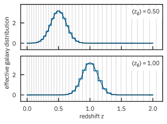
Figure 7: Effective redshift distribution (blue) of the discretised galaxy density contrast $\delta^{\mathrm{g}}_{i}$ for two representative populations (black) with mean redshifts $\langle z_{\mathrm{g}}\rangle=0.5$ (top) and $\langle z_{\mathrm{g}}\rangle=1.0$ (bottom). Vertical lines indicate the boundaries of matter shells with constant thickness in comoving distance $\Delta d_{\mathrm{c}}=150$ Mpc.

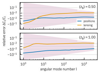
Figure 8: The relative error in the angular power spectra for the effective galaxy distribution of the discretised galaxy field, as shown in Figure 7, for positions (blue) and lensing (orange). The shaded area shows the standard deviation of a Gaussian field for comparison.

Because we sample galaxy positions from the discretised galaxy density contrast $\delta^{\mathrm{g}}_{i}$, all galaxies in a given shell $i$ follow the same matter density field $\delta_{i}$, given by the projection (2). As far as the two-point statistics are concerned, the effective redshift distribution of the galaxies in shell $i$ is therefore determined by the matter weight function $W_{i}$. This is shown in Figure 7 for shells of size $\Delta d_{\mathrm{c}}=150$ Mpc in comoving distance, and two representative Gaussian redshift distributions with respective means $z=0.5$ and $z=1.0$ and the same standard deviation $\sigma_{z}=0.125$. Although the situation is ostensibly similar to the lensing kernels in Figure 5, the smaller size of the distributions compared to the shells results in relative errors at the per cent level in the angular power spectra for the galaxy positions and lensing, shown in Figure 8. However, this level of uncertainty in the galaxy distribution is comparable to that achieved by observations (Tanaka et al., 2018; Graham et al., 2018; Euclid Collaboration et al., 2020; Hildebrandt et al., 2021; Cordero et al., 2022), so that there is little real incentive to push the errors down by decreasing the shell size. In fact, the observational uncertainty means that we can simply assume the discretised distribution in Figure 7 to be the true redshift distribution of our simulated survey, without introducing a significant disagreement between simulations and observations. If we apply this strategy, errors from the discretisation of the matter fields disappear entirely in the galaxies sector, for both angular clustering and weak lensing.

5.2 Galaxy redshifts

For the radial distribution of galaxies, we sample the true redshift $z$ of galaxies from a given redshift distribution $dN/dz$, with $N$ the number density of galaxies as a function of redshift. This is done separately within each matter shell. Although the resulting galaxy redshifts will follow the given distribution, they will not display any radial correlations on scales smaller than the matter shells. The choice of redshift distribution is arbitrary, and could be the actual distribution from a galaxy survey, or the commonly used distribution of Smail et al. (1994) for photometric surveys,

$$p(z)\propto z^{\alpha}\,\mathrm{e}^{-(z/z_{0})^{\beta}}\;,$$ (61)

where $z_{0}$ is related to the median redshift of the distribution, while the exponents $\alpha$ and $\beta$ are typically set to 2 and 1.5, respectively (Amara & Réfrégier, 2007). We allow for multiple such redshift distributions to be given, which might represent different samples or tracers of large-scale structure.

We can additionally generate photometric galaxy redshifts $z_{\mathrm{ph}}$ by sampling from a conditional redshift distribution $p(z_{\rm ph}|z)$. For example, a redshift-dependent Gaussian error with standard deviation $\sigma(z)=\sigma_{0}\,(1+z)$, parametrised by the error $\sigma_{0}$ at $z=0$, has the conditional distribution

$$p(z_{\mathrm{ph}}|z)=\frac{1}{\sigma(z)\,\sqrt{2\pi}}\exp\Bigl{\{}-\frac{1}{2}\,\Bigl{(}\frac{z_{\mathrm{ph}}-z}{\sigma(z)}\Bigr{)}^{2}\Bigr{\}}\;,$$ (62)

which is readily numerically sampled. If a more realistic and tailored simulation is desired, any other conditional distribution can be used in place of this simple model, such as e.g. the empirical photometric redshift distribution of a given survey.

Finally, we note that both the true and the photometric redshift distributions do not have to coincide at all with the matter shells, and can have arbitrary overlaps.

5.3 Galaxy shears

One of the main cosmological observables in galaxy surveys is the shape of objects. It is quantified by the ellipticity $\epsilon$, which is complex-valued with components $\epsilon_{1}$ and $\epsilon_{2}$,

$$\epsilon=\epsilon_{1}+\mathrm{i}\,\epsilon_{2}\;.$$ (63)

The simplest case is the ellipticity of an elliptical isophote with axis ratio $q$, rotated by an angle $\phi$ against the local coordinate frame,

$$\epsilon=\frac{1-q}{1+q}\,\mathrm{e}^{2\mathrm{i}\phi}\;.$$ (64)

For extended surface brightness distributions, the ellipticity is defined in terms of the second moments of the distribution (see e.g. Schneider et al., 2006). It is strictly true that $|\epsilon|\leq 1$, which follows immediately from (64) for an elliptical isophote, and from positive definiteness of the second moments in the general case.

The importance of the ellipticity $\epsilon$ for cosmology is owed to the fact that it is a tracer of the so-called reduced shear $g$, which is a complex-valued field that combines the convergence $\kappa$ and shear $\gamma$ from weak gravitational lensing,

$$g=\frac{\gamma}{1-\kappa}\;.$$ (65)

Under the influence of a reduced shear $g$, the ellipticity $\epsilon$ of a small source transforms as

$$\epsilon\mapsto\frac{\epsilon+g}{1+g^{*}\epsilon}\;.$$ (66)

It was shown by Seitz & Schneider (1997) that if the unlensed galaxy ellipticity distribution is isotropic, i.e. with no preferred direction, then the expectation of the ellipticity $\epsilon$ equals the reduced shear $g$,

$$\langle\epsilon\rangle=g\;.$$ (67)

Although this result is often stated as an approximation to first order in $g$ (which it is not), it holds exactly for any isotropic distribution of galaxy ellipticities. If we only care for galaxy ellipticities as tracers of the weak lensing field, we thus have the freedom to choose any such distribution for our simulation.

A common choice is to sample the ellipticity components $\epsilon_{1}$ and $\epsilon_{2}$ as independent normal random variates with a given standard deviation $\sigma_{\epsilon}$ in each component. We present this model, as well as a related but improved distribution, in Appendix C. For a more realistic ellipticity distribution, we can sample the galaxy shape e.g. as a triaxial ellipsoid under a random viewing angle (Ryden, 2004). In this way, it is also possible to include even more subtle effects such as e.g. dust extinction and reddening, which depend on the viewing angle of the galaxy (Padilla & Strauss, 2008).

For any chosen distribution, we sample an ellipticity for each galaxy in a given shell $i$. We then interpolate the convergence map $\kappa_{i}$ and shear map $\gamma_{i}$ at the galaxy position. From these values, we compute the reduced shear (65) and use the transformation law (66) to give each galaxy an observed ellipticity under the effect of weak lensing. As commonly done, we call the weakly-lensed ellipticities the “galaxy shears”.

5.4 Intrinsic alignments

Galaxies systematically align with the overall large-scale structure of the universe (for reviews, see Joachimi et al., 2015; Kiessling et al., 2015; Kirk et al., 2015). This effect breaks the assumed isotropy of the distribution of galaxy shapes, and translates into correlations in the ellipticities between physically close galaxies. On the level of two-point statistics, the result is a contamination of the cosmic shear signal by so-called intrinsic alignments (Heavens et al., 2000; King & Schneider, 2002; Heymans & Heavens, 2003; Bridle & King, 2007).

However, the fact that the signals from weak lensing and intrinsic alignments are very similar can be exploited for simulations (Hikage et al., 2019; Gatti et al., 2020; Asgari et al., 2021; Jeffrey et al., 2021). If we adjust the convergence $\kappa$ from weak lensing to include an effective contribution $\kappa^{\mathrm{IA}}$ from intrinsic alignments,

$$\kappa\mapsto\kappa+\kappa^{\mathrm{IA}}\;,$$ (68)

this is subsequently transformed into an effective shear via (57), and the resulting reduced shear (65) imprints the correlation due to intrinsic alignments onto the isotropic galaxy ellipticities at the same time as the shear. To simulate intrinsic alignments in this manner, we add $\kappa^{\mathrm{IA}}$ to our $\kappa$ map before the galaxy ellipticities are sampled (but after all simulation steps that require the true convergence have passed).

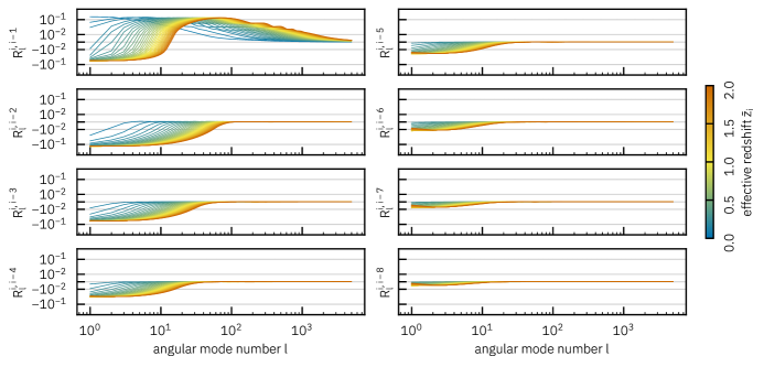
Figure 9: Correlation coefficient $R_{l}^{ij}$ for the angular matter power spectrum of shells with constant thickness $\Delta d_{\mathrm{c}}=150$ Mpc in comoving distance. Shown are consecutive shells with $j-i=1$ (top left) to $j-i=8$ (bottom right). The colours indicate the effective redshift of each shell from $z=0$ to $z=2$.

To give a specific example, a widely used model to obtain the effective convergence (68) is the Non-Linear Alignment (NLA) model (Catelan et al., 2001; Hirata & Seljak, 2004; Bridle & King, 2007). It proposes that the shear signal coming from intrinsic alignments is proportional to the projected tidal field and hence ultimately to the matter density contrast $\delta$. For a given shell $i$, we compute the effective contribution $\kappa^{\mathrm{IA}}_{i}$ in (68) from the projected matter field $\delta_{i}$,

$$\kappa^{\mathrm{IA}}_{i}(\hat{u})\\ =-A_{\mathrm{IA}}\,\frac{C_{1}\,\Omega_{\mathrm{m}}\,\overline{\rho}_{\mathrm{cr}}(\bar{z}_{i})}{D(\bar{z}_{i})}\,\bigg{(}\frac{1+\bar{z}_{i}}{1+z_{\mathrm{IA}}}\bigg{)}^{\eta(\bar{z}_{i})}\,\delta_{i}(\hat{u})\;,$$ (69)

where $A_{\mathrm{IA}}$ is the intrinsic alignment amplitude, $C_{1}$ is a normalisation constant (Hirata & Seljak, 2004), $\overline{\rho}_{\mathrm{cr}}(\bar{z}_{i})$ is the mean critical matter density of the universe at a representative redshift $\bar{z}_{i}$ for shell $i$, $D(\bar{z}_{i})$ is the growth factor normalised to unity today, and $\eta$ is the index of a power law which describes the redshift dependence of the intrinsic alignment strength relative to the tidal field with respect to the pivot redshift $z_{\mathrm{IA}}$.

6 Simulating a weak lensing galaxy survey

We have implemented the simulation steps of the previous sections in a new, publicly available computer code called GLASS, the Generator for Large Scale Structure. In this section, we use GLASS to demonstrate a simulation that would be typical for a Stage 4 photometric weak lensing galaxy survey such as Euclid, LSST, or Roman.

Our initial Figure 1 provides a high-level flowchart for how GLASS simulates individual shells. In the matter sector, we specify the shell boundaries and the matter weight functions, from which the angular matter power spectra are computed. For this example, we once again use CAMB, without Limber’s approximation. A lognormal matter field is subsequently sampled from the angular matter power spectra, using a chosen number of previous shells for correlations.

In the weak lensing sector, the matter weight functions are used to compute the lensing weights (46). The lensing weights and the matter field are then used to iteratively compute the convergence field. If intrinsic alignments of galaxies are being simulated, their effect is added to the convergence field. Finally, the shear field is computed from the convergence using a spherical harmonic transform.

In the galaxies sector, the matter field is biased to sample the random galaxy positions. Galaxy redshifts are sampled directly from the provided source distributions. Galaxy ellipticities are sampled from a suitable distribution. Positions and ellipticities then enter the computation of the galaxy shears: The convergence and shear fields are interpolated using the galaxy redshifts and evaluated at the galaxy positions to produce the reduced shears, which is applied to the galaxy ellipticities to produce the final galaxy shears.

The outcome of these steps is a typical galaxy catalogue with positions, redshifts, and shears, which can be used for what is often called “3x2pt” analysis.

We will now carry out a simulation to validate these results, which requires a number of user choices. The first is the distribution of the matter shell boundaries, and hence the size of the shells. Because the two-point statistics of the matter field ultimately depend on physical distance, we generally choose matter shells with a constant size in comoving distance. As shown in Sections 4 and 5, we obtain accurate results from the respective approximations for lensing and galaxies when the matter fields are discretised in shells of a constant size of $\Delta d_{\mathrm{c}}=150$ Mpc in comoving distance. We therefore adopt this value here.

As explained in Section 3, we can then choose to only keep a limited number of correlated matter shells in memory over the course of the simulation, to reduce the computational burden imposed by such thin shells. To make an informed choice for said number, we quantify the correlation of the matter fields between two shells $i$ and $j$ by introducing the correlation coefficient $R_{l}^{ij}$ of the angular matter power spectra,

$$R_{l}^{ij}=\frac{C_{l}^{ij}}{\sqrt{C_{l}^{ii}\,C_{l}^{jj}}}\;.$$ (70)

Angular power spectra are the (co)variances of the modes of the spherical harmonic expansion, and $R_{l}^{ij}$ is hence a proper correlation coefficient in the usual sense: It takes values between $+1$ and $-1$, with the former meaning perfect correlation, and the latter meaning perfect anticorrelation. Figure 9 shows the correlation coefficient $R_{l}^{ij}$ for offsets $j-i=1,\ldots,8$ in shells with $\Delta d_{\mathrm{c}}=150$ Mpc at redshifts between $0$ and $2$. We see how the correlation between shells scans through the three-dimensional matter correlation function: On scales $\lesssim 150$ Mpc comoving, matter is largely positively correlated, which is seen in adjacent shells. This is compensated by negative correlation on larger scales, which is seen in the non-neighbouring shells.

We now consult Figure 9 to find the number of matter shells to correlate. If we wish to achieve per cent-level accuracy in the matter sector at $l\approx 10$, say, we find that it suffices to keep five correlated shells in memory over the entire redshift range, which is readily achievable on standard computer hardware. This level of accuracy is consistent with the lensing sector, shown in Figure 6, and the galaxies sector, shown in Figure 8. We can therefore make simple and understandable choices about the simulation parameters, based on the desired accuracy of the results. Of course, the specific values we use depend entirely on our adopted shell size of $\Delta d_{\mathrm{c}}=150$ Mpc.

To demonstrate that the realised matter field achieves our stated accuracy, we create $200$ simulations of lognormal matter fields with angular modes up to $l=5\,000$ from HEALPix maps with $N_{\mathrm{side}}=4\,096$. Figure 10 shows the mean relative error of the realised angular matter power spectra for three representative shells with redshifts near $z=0.5$, $z=1.0$, and $z=2.0$. The achieved error is well below the per cent level, which in turn is well below the level of cosmic variance of the realisations. This level of accuracy in the recovered matter fields is not currently attained by lognormal simulations (Xavier et al., 2016), which shows that our Gaussian angular power spectrum solver is working as intended.

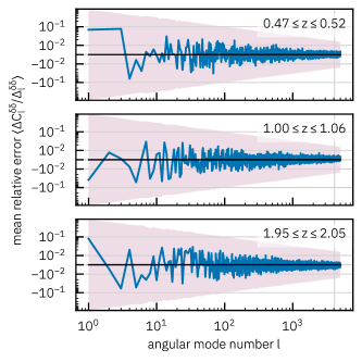
Figure 10: Mean relative error of the angular matter power spectra from 200 realisations of a lognormal matter field. Shown are three shells containing redshifts $z$ with $0.47\leq z\leq 0.52$ (top), $1.00\leq z\leq 1.06$ (middle), and $1.95\leq z\leq 2.05$ (bottom). The vertical line indicates the $N_{\mathrm{side}}$ parameter of the simulation. The shaded area shows cosmic variance of the realisations.

Using the same $200$ realisations, we also demonstrate that the iterative computation of the convergence field with the multi-plane formalism (45) achieves the desired accuracy. Figure 11 shows the mean relative error of the realised angular power spectra for three source redshifts near $z=0.5$, $z=1.0$, and $z=2.0$. The realisations agree with the theoretical predictions from Figure 6 up to the point near $l\approx 10$ where missing (anti-)correlations from the uncorrelated shells become significant, according to Figure 9. This missing negative correlation explains why, for values of $l\lesssim 10$, the simulated convergences have angular power spectra which lie above the expectations. Overall, the results of Figure 11 hence show not only that the multi-plane approximation for weak lensing holds, but also that cross-correlations are correctly imprinted on the matter fields.

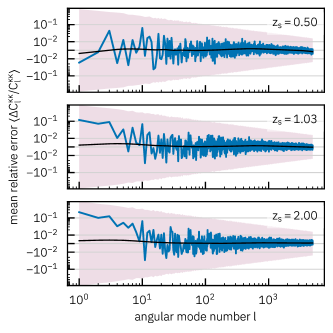
Figure 11: Mean relative error of the angular power spectra of the convergence from 200 realisations of a lognormal matter field with five correlated shells (blue). Shown are source redshifts $z_{\mathrm{s}}=0.50$ (top), $z_{\mathrm{s}}=1.03$ (middle), and $z_{\mathrm{s}}=2.00$ (bottom). Also shown is the expected curve from Figure 6 for fully correlated shells (black). The shaded area shows cosmic variance of the realisations.

As a final test, we simulate a catalogue of galaxies that is typical for “3x2pt” analysis with tomographic redshift bins. Since we are only interested in validation here, we use two redshift bins with small but not insignificant overlap, which is the case where cross-correlations are most difficult to get right. In particular, we adopt the discretised distribution of Figure 7 as the true galaxy distribution, so that we can expect there to be no effect due to discretisation on our results. We generate $1\,000$ simulations of galaxy positions, redshifts, and shears, using a mean number density of 1 galaxy per square arcminute in each tomographic bin. To be able to compute accurate theoretical predictions for the results, we use a linear galaxy bias with constant bias parameter $b=0.8$. This unrealistically low value $b<1$ is necessary for accuracy of the theory, not our simulations: If $b>1$, the galaxy density contrast $\delta_{\mathrm{g}}=b\,\delta$ can become less than $-1$ in very underdense regions. We would have to clip such unphysical values to $-1$ in our simulation, which effectively renders the model non-linear, and deviates from the assumed theory.

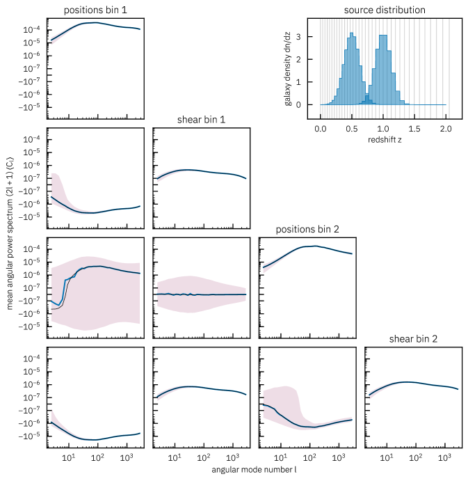
Figure 12: Mean angular power spectra (blue) from $1\,000$ realisations of galaxy positions and shears in a simulated full-sky survey. Shown are the auto- and cross-correlations for two tomographic redshift bins 1 and 2 with respective mean redshifts of $\langle z\rangle=0.5$ and $\langle z\rangle=1.0$ (inset). Also shown are the theoretical spectra computed by CAMB (black). To reduce visible noise, the angular power spectra are averaged over 40 logarithmic bins in angular mode number $l$. The shaded area shows cosmic variance of the realisations.

For every combination of galaxy positions and shears across the two bins, we then compare the realised angular power spectra to theory. The results are shown in Figures 12 and 13. For validation, we show shear signals computed from the full-sky weak lensing maps, so that we do not have to account for the effect of shot noise from the galaxy positions, which is difficult to model theoretically at our intended level of accuracy. Another difficulty is the reduced shear approximation (Krause & Hirata, 2010; Deshpande et al., 2020): galaxies trace the reduced shear (65), whereas theory codes in general only compute the angular power spectrum of the convergence or shear field. The difference between the two cases is readily seen in our simulations, as shown in Figure 13. For an accurate evaluation of our results, we must therefore compare the shear, and not the reduced shear, with the theoretical values computed by CAMB. Overall, we find very good agreement at the sub-per cent level, in line with our expectations.

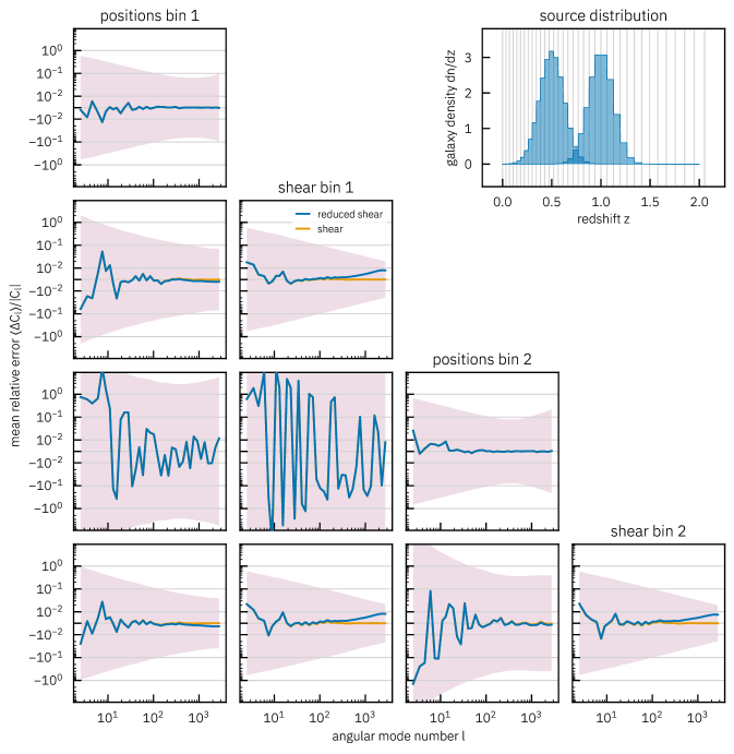
Figure 13: Mean relative error between the measured and theoretical angular power spectra of Figure 12. Shown are results for both the reduced shear $g$ (blue), of which galaxies are a tracer, and the true shear $\gamma$ (orange), which is the fundamental gravitational lensing field. The theoretical spectra from CAMB are computed for the latter instead of the former. The shaded area shows cosmic variance of the realisations. The central panel is essentially pure noise because there is only a vanishingly small correlation between shear in the foreground and positions in the background.

7 Discussion & Conclusions

We have introduced GLASS, the Generator for Large Scale Structure, which is a public code for creating simulations of wide-field galaxy surveys, with a particular focus on weak gravitational lensing. Our simulated light cones are built as a series of nested matter shells around the observer, iteratively sampled from a given statistical distribution. If the matter field can be approximated as uncorrelated beyond a certain length scale, which is a fair approximation, our simulations can be carried out with constant memory use. This allows us in principle to simulate any number of matter shells, and therefore to achieve a much higher resolution than currently possible in both the radial and angular dimensions. As a result, our method readily achieves per cent-level accuracy for clustering and weak lensing two-point statistics for angular mode numbers $l\gtrsim 3\,000$ and redshifts $z\gtrsim 2$, which are typical for Stage 4 photometric galaxy surveys.

A key part in that is a novel way to realise transformed Gaussian random fields, such as e.g. lognormal fields, with angular power spectra of a given angular range and practically arbitrary accuracy and precision. Moreover, we developed a scheme to compute the weak lensing convergence field iteratively, using a multi-plane formalism usually employed in strong gravitational lensing. The accuracy of the weak lensing fields is essentially determined by the size of the matter shells, and can therefore be controlled as necessary for a given simulation. The situation is similar for angular galaxy clustering, which is more sensitive to the relative resolution of the matter shells compared to the width of the galaxy redshift distribution. Overall, the ability to increase the radial resolution, and hence number of matter shells, without quadratically increasing memory use, is therefore crucial.

GLASS is fast: the high-precision matter, galaxy clustering, and lensing simulations we present take around 30 minutes wall-clock time each on standard 8-core computing nodes, including analysis of the results. Another benefit of the iterative computation in shells is that results are available for processing as soon as each new shell is computed. Therefore, simulation and analysis pipelines can be constructed in which no large amounts of data (e.g. catalogues or maps) are ever written to disk. This is particularly important since the speed and resource efficiency of GLASS can lead to input and output becoming a limiting factor in such pipelines.

Our approach of a hybrid mix of statistical and physical models allows for simulations in which each individual step is understandable, analysable, and extensible, providing the simulator with control over the trade-off between accuracy and speed/resource consumption. The GLASS design is completely modular, and without a “default mode” of operation; all models we present in this work, including the most basic ones for matter and lensing, are readily replaced or expanded. This makes GLASS a well-suited tool for stress-testing and validating the processing and analysis pipelines of galaxy surveys.

We demonstrated that the GLASS simulator matches or exceeds the accuracy of our current analytic models of the dark matter distribution (c.f. Euclid Collaboration et al., 2019; Mead et al., 2021). Hence, simulation-based inference of two-point statistics employing GLASS will be at least as accurate as traditional analytic approaches, but offers a much more straightforward route to addressing otherwise formidable analysis challenges, such as non-Gaussian likelihoods, higher-order signal corrections, complex galaxy sample selection, and spatially varying survey properties, to name just a few. In forthcoming work we will extend the GLASS approach to also produce highly accurate higher-order statistics of the matter distribution to enable their simultaneous inference.

Acknowledgements

We would like to thank A. Hall for his always very helpful comments and insights, as well as the anonymous reviewer for their constructive comments which improved this text.

NT, AL, and BJ are supported by UK Space Agency grants ST/W002574/1 and ST/X00208X/1. BJ is also supported by STFC Consolidated Grant ST/V000780/1. MvWK acknowledges STFC for support in the form of a PhD Studentship.

We gratefully acknowledge use of the following software packages: NumPy (Harris et al., 2020), HEALPix (Górski et al., 2005), healpy (Zonca et al., 2019), and Matplotlib (Hunter, 2007).

Data availability

All data and software used in this article is publicly available. GLASS is open source software and its repository and documentation can be found online. The scripts to generate the simulations and plots presented here can be found in a separate software repository. All Python packages mentioned in the text can be obtained from the Python Package Index.

Appendix A Discrete Legendre Transform

The transformation (15) and (16) between angular power spectra and angular correlation functions is essentially the Legendre expansion of the function $C(\theta)$. To compute it for inputs of finite length, we use a recursive algorithm, based on the starting point for the algorithms of Alpert & Rokhlin (1991). The main idea is as follows. If a function $f$ has a finite Legendre expansion of the form

$$f(\theta)=\sum_{l=0}^{n-1}a_{l}\,P_{l}(\cos\theta)\;,$$ (71)

then it also has a finite Fourier cosine expansion of the form

$$f(\theta)=\sum_{k=0}^{n-1}b_{k}\cos(k\theta)\;,$$ (72)

since $P_{l}(\cos\theta)$ is a polynomial of degree $l$ in $\cos\theta$. The coefficient vectors $\bm{a}=\{a_{0},\ldots,a_{n-1}\}$ and $\bm{b}=\{b_{0},\ldots,b_{n-1}\}$ are related as $\bm{b}=\mathrm{\mathbf{M}}\bm{a}$, where the matrix $\mathrm{\mathbf{M}}$ has entries

$$M_{ij}=\begin{cases}\frac{1}{\pi}\,\frac{\Gamma(\frac{j+1}{2})^{2}}{\Gamma(\frac{j+2}{2})^{2}}&\text{if $0=i\leq j<n$ and $j$ even,}\\[10.0pt] \frac{2}{\pi}\,\frac{\Gamma(\frac{j-i+1}{2})\,\Gamma(\frac{j+i+1}{2})}{\Gamma(\frac{j-i+2}{2})\,\Gamma(\frac{j+i+2}{2})}&\text{if $0<i\leq j<n$ and $i+j$ even,}\\[10.0pt] 0&\text{otherwise,}\end{cases}$$ (73)

and $\Gamma$ is the gamma function. Conversely, if $f$ has a finite Fourier cosine expansion (72), then it also has a finite Legendre expansion (71), and the coefficient vectors are related as $\bm{a}=\mathrm{\mathbf{L}}\bm{b}$, where the matrix $\mathrm{\mathbf{L}}$ has entries

$$L_{ij}=\begin{cases}1&\text{if $i=j=0$,}\\[10.0pt] \frac{\sqrt{\pi}}{2}\,\frac{\Gamma(\frac{2i+2}{2})}{\Gamma(\frac{2i+1}{2})}&\text{if $0<i=j<n$,}\\[10.0pt] \frac{-j\,(i+\frac{1}{2})}{(j+i+1)\,(j-i)}\,\frac{\Gamma(\frac{j-i-1}{2})\,\Gamma(\frac{j+i}{2})}{\Gamma(\frac{j-i}{2})\,\Gamma(\frac{j+i+1}{2})}&\text{if $0\leq i<j<n$ and $i+j$ even,}\\[10.0pt] 0&\text{otherwise.}\end{cases}$$ (74)

Since the transformation between coefficient vector $\bm{b}$ and function values $f(\theta)$ can be done efficiently with a Discrete Cosine Transform (DCT), the Discrete Legendre Transform (DLT) reduces to a DCT and matrix multiplication $\bm{a}=\mathrm{\mathbf{L}}\bm{b}$; and the inverse DLT reduces to a matrix multiplication $\bm{b}=\mathrm{\mathbf{M}}\bm{a}$ and inverse DCT.

With fast algorithms for the DCT widely available, our task reduces to computing the matrix products with $\mathrm{\mathbf{L}}$ and $\mathrm{\mathbf{M}}$. Although the main result of Alpert & Rokhlin (1991) was an efficient algorithm for this purpose, here we use a simple recurrence to compute $\mathrm{\mathbf{M}}\bm{a}$ or $\mathrm{\mathbf{L}}\bm{b}$ without explicitly constructing a large matrix. The recursive computation does not have the same algorithmic complexity as the method proposed by Alpert & Rokhlin (1991), but is nevertheless very fast due to its simplicity.

The entries (73) of $\mathrm{\mathbf{M}}$ can alternatively be specified by the first two diagonal elements $M_{00}=M_{11}=1$, from which all subsequent diagonal elements $M_{ii}$, $i>1$, can be computed as

$$M_{ii}=\Bigl{(}1-\frac{1}{2i}\Bigr{)}\,M_{i-1,i-1}\;.$$ (75)

The lower triangle of the matrix is identically zero. Above the diagonal, the values $M_{ij}$ for $j>i$ can be computed as

$$M_{ij}=\Bigl{(}1-\frac{1}{j-i}\Bigr{)}\,\Bigl{(}1-\frac{1}{j+i}\Bigr{)}\,M_{i,j-2}\;.$$ (76)

The first off-diagonal and every other subsequent entry vanishes ($i+j$ odd).

The entries (74) of $\mathrm{\mathbf{L}}$ can be computed similarly by starting the diagonal with $L_{00}=L_{11}=1$ and continuing as

$$L_{ii}=\frac{1}{1-\frac{1}{2i}}\,L_{i-1,i-1}\;.$$ (77)

The lower triangle is again zero, and the values $L_{ij}$ for $j>i$ can be computed as

$$L_{ij}=\Bigl{(}1+\frac{2}{j-2}\Bigr{)}\,\Bigl{(}1-\frac{3}{j-i}\Bigr{)}\,\Bigl{(}1-\frac{3}{j+i+1}\Bigr{)}\,L_{i,j-2}\;.$$ (78)

As before, the first off-diagonal and every other subsequent entry vanishes ($i+j$ odd).

Appendix B Iterative multivariate normal random sampling

Let $\bm{x}_{n+1}=\{x_{1},\ldots,x_{n+1}\}$ be a multivariate normal random vector of length $n+1$ with mean $\bm{\mu}_{n+1}=\{\mu_{1},\ldots,\mu_{n+1}\}$ and covariance matrix $\mathrm{\mathbf{\Sigma}}_{n+1}$. The vector $\bm{x}_{n}$ of the first $n$ variates is then a multivariate normal random vector with mean $\bm{\mu}_{n}$ and covariance matrix $\mathrm{\mathbf{\Sigma}}_{n}$, which is the leading $n\times n$ submatrix of $\mathrm{\mathbf{\Sigma}}_{n+1}$. Given a sample $\bm{x}_{n}$ from its marginal distribution, what is the conditional distribution of $x_{n+1}$?

Of course, this is a classical problem with a well-known solution: Writing the covariance matrix $\mathrm{\mathbf{\Sigma}}_{n+1}$ in block matrix form as

$$\mathrm{\mathbf{\Sigma}}_{n+1}=\begin{bmatrix}\mathrm{\mathbf{\Sigma}}_{n}&\bm{c}_{n}\\ \bm{c}_{n}^{\mkern-0.5mu\mathsf{T}}&\sigma^{2}_{n+1}\end{bmatrix}\;,$$ (79)

the conditional distribution of $x_{n+1}$ is normal with mean

$$\tilde{\mu}_{n+1}=\mu_{n+1}+\bm{c}_{n}^{\mkern-0.5mu\mathsf{T}}\,\mathrm{\mathbf{\Sigma}}_{n}^{-1}\,(\bm{x}_{n}-\bm{\mu}_{n})$$ (80)

and variance

$$\tilde{\sigma}^{2}_{n+1}=\sigma^{2}_{n+1}-\bm{c}_{n}^{\mkern-0.5mu\mathsf{T}}\,\mathrm{\mathbf{\Sigma}}_{n}^{-1}\,\bm{c}_{n}\;.$$ (81)

We can hence sample from a multivariate normal distribution by sampling each individual normal variate in turn, using the conditional mean (80) and variance (81).

In fact, the entire sampling process can be performed iteratively. Let $\mathrm{\mathbf{A}}_{n}$ be the Cholesky decomposition of $\mathrm{\mathbf{\Sigma}}_{n}^{-1}$ such that $\mathrm{\mathbf{\Sigma}}_{n}^{-1}=\mathrm{\mathbf{A}}_{n}^{\mkern-0.5mu\mathsf{T}}\,\mathrm{\mathbf{A}}_{n}$. We can write the conditional mean (80) and variance (81) as

$$\tilde{\mu}_{n+1}=\mu_{n+1}+\bm{a}_{n}^{\mkern-0.5mu\mathsf{T}}\,\bm{y}_{n}\;,$$ (82)

$$\tilde{\sigma}^{2}_{n+1}=\sigma^{2}_{n+1}-\bm{a}_{n}^{\mkern-0.5mu\mathsf{T}}\,\bm{a}_{n}\;,$$ (83)

where we have introduced vectors $\bm{a}_{n}=\mathrm{\mathbf{A}}_{n}\,\bm{c}_{n}$ and $\bm{y}_{n}=\mathrm{\mathbf{A}}_{n}\,(\bm{x}_{n}-\bm{\mu}_{n})$. Since $\mathrm{\mathbf{A}}_{n}^{\mkern-0.5mu\mathsf{T}}\,\mathrm{\mathbf{A}}_{n}=\mathrm{\mathbf{\Sigma}}_{n}^{-1}$, the vector $\bm{y}_{n}$ contains the $n$ standard normal random variates of the whitened given sample. It is updated by appending each new standard normal variate $y_{n+1}=(x_{n+1}-\tilde{\mu}_{n+1})/\tilde{\sigma}_{n+1}$ as it is drawn,

$$\bm{y}_{n+1}=\begin{pmatrix}\bm{y}_{n}\\ y_{n+1}\end{pmatrix}\;.$$ (84)

To obtain the conditional mean and variance, we therefore only have to compute the vector $\bm{a}_{n}$ explicitly. To do so, we require $\mathrm{\mathbf{A}}_{n}$.

Writing the matrix $\mathrm{\mathbf{\Sigma}}_{n}$ in block matrix form (79), the inverse $\mathrm{\mathbf{\Sigma}}_{n}^{-1}$ can be computed using block matrix inversion, and factorised as

$$\mathrm{\mathbf{\Sigma}}_{n}^{-1}=\begin{pmatrix}\mathrm{\mathbf{I}}&-\mathrm{\mathbf{\Sigma}}_{n-1}^{-1}\,\bm{c}_{n-1}\\ \mathrm{\mathbf{0}}&\mathrm{\mathbf{I}}\end{pmatrix}\,\begin{pmatrix}\mathrm{\mathbf{\Sigma}}_{n-1}^{-1}&\mathrm{\mathbf{0}}\\ \mathrm{\mathbf{0}}&\tilde{\sigma}^{-2}_{n}\end{pmatrix}\,\begin{pmatrix}\mathrm{\mathbf{I}}&\mathrm{\mathbf{0}}\\ -\bm{c}_{n-1}^{\mkern-0.5mu\mathsf{T}}\,\mathrm{\mathbf{\Sigma}}_{n-1}^{-1}&\mathrm{\mathbf{I}}\end{pmatrix}\;,$$ (85)

where $\mathrm{\mathbf{I}}$ and $\mathrm{\mathbf{0}}$ are the identity and zero matrix, respectively, of the appropriate shape. Looking at (85), the updating rule for $\mathrm{\mathbf{A}}_{n}$ is readily obtained,

$$\mathrm{\mathbf{A}}_{n}=\begin{pmatrix}\mathrm{\mathbf{A}}_{n-1}&\mathrm{\mathbf{0}}\\ -\tilde{\sigma}_{n}^{-1}\,\bm{a}_{n-1}^{\mkern-0.5mu\mathsf{T}}\,\mathrm{\mathbf{A}}_{n-1}&\tilde{\sigma}_{n}^{-1}\end{pmatrix}\;.$$ (86)

It is clear that $\mathrm{\mathbf{A}}_{n}$ grows by one row and one column in each iteration, and is a lower triangular matrix for all $n$.

To sample $x_{n+1}$ iteratively, we hence need to store the $n$ standard normal variates $\bm{y}_{n}$ and the $n\times n$ matrix $\mathrm{\mathbf{A}}_{n}$. However, the storage requirements reduce from $n$ to $k$ if each new random variable $x_{n+1}$ only correlates with the last $k$ random variates $x_{n-k+1},\ldots,x_{n}$. The covariance matrix $\mathrm{\mathbf{\Sigma}}_{n+1}$ is then a banded matrix, so that the vector $\bm{c}_{n}$ has $n-k$ leading zeros. In block matrix form,

$$\bm{c}_{n}=\begin{pmatrix}\bm{0}\\ \tilde{\bm{c}}_{n}\end{pmatrix}\;,$$ (87)

where $\tilde{\bm{c}}_{n}$ is the reduced vector of $k$ non-zero correlations. The lower triangular matrix $\mathrm{\mathbf{A}}_{n}$ can be written in block matrix form as

$$\mathrm{\mathbf{A}}_{n}=\begin{pmatrix}\mathrm{\mathbf{U}}_{n}&\mathrm{\mathbf{0}}\\ \mathrm{\mathbf{V}}_{n}&\tilde{\mathrm{\mathbf{A}}}_{n}\end{pmatrix}\;,$$ (88)

where $\tilde{\mathrm{\mathbf{A}}}_{n}$ is the lower $k\times k$ block of $\mathrm{\mathbf{A}}_{n}$, with $\mathrm{\mathbf{U}}_{n}$, $\mathrm{\mathbf{V}}_{n}$ the remaining blocks. It follows that the vector $\bm{a}_{n}=\mathrm{\mathbf{A}}_{n}\,\bm{c}_{n}$ will also have $n-k$ leading zeros, since

$$\bm{a}_{n}=\begin{pmatrix}\mathrm{\mathbf{U}}_{n}&\mathrm{\mathbf{0}}\\ \mathrm{\mathbf{V}}_{n}&\tilde{\mathrm{\mathbf{A}}}_{n}\end{pmatrix}\,\begin{pmatrix}\bm{0}\\ \tilde{\bm{c}}_{n}\end{pmatrix}=\begin{pmatrix}\bm{0}\\ \tilde{\mathrm{\mathbf{A}}}_{n}\,\tilde{\bm{c}}_{n}\end{pmatrix}=\begin{pmatrix}\bm{0}\\ \tilde{\bm{a}}_{n}\end{pmatrix}\;,$$ (89)

where $\tilde{\bm{a}}_{n}=\tilde{\mathrm{\mathbf{A}}}_{n}\,\tilde{\bm{c}}_{n}$ is the non-zero part of $\bm{a}_{n}$ of length $k$. The conditional mean (82) and variance (83) can hence be written

$$\tilde{\mu}_{n+1}=\mu_{n+1}+\tilde{\bm{a}}_{n}^{\mkern-0.5mu\mathsf{T}}\,\tilde{\bm{y}}_{n}\;,$$ (90)

$$\tilde{\sigma}^{2}_{n+1}=\sigma^{2}_{n+1}-\tilde{\bm{a}}_{n}^{\mkern-0.5mu\mathsf{T}}\,\tilde{\bm{a}}_{n}\;,$$ (91)

where $\tilde{\bm{y}}_{n}$ is the reduced vector of the last $k$ standard normal variates. Writing the update (86) of the matrix $\mathrm{\mathbf{A}}_{n}$ in terms of reduced quantities,

$$\mathrm{\mathbf{A}}_{n}=\begin{pmatrix}\mathrm{\mathbf{U}}_{n-1}&\mathrm{\mathbf{0}}&\mathrm{\mathbf{0}}\\ \mathrm{\mathbf{V}}_{n-1}&\tilde{\mathrm{\mathbf{A}}}_{n-1}&\mathrm{\mathbf{0}}\\ -\tilde{\sigma}_{n}^{-1}\,\tilde{\bm{a}}_{n-1}^{\mkern-0.5mu\mathsf{T}}\,\mathrm{\mathbf{V}}_{n-1}&-\tilde{\sigma}_{n}^{-1}\,\tilde{\bm{a}}_{n-1}^{\mkern-0.5mu\mathsf{T}}\,\tilde{\mathrm{\mathbf{A}}}_{n-1}&\tilde{\sigma}_{n}^{-1}\end{pmatrix}\;,$$ (92)

it is clear that only the lower $k\times k$ submatrix $\tilde{\mathrm{\mathbf{A}}}_{n}$ needs to be computed and stored. Its update can be written as

$$\begin{pmatrix}\;\cdot\;&\cdots\\ \vdots&\tilde{\mathrm{\mathbf{A}}}_{n}\end{pmatrix}=\begin{pmatrix}\tilde{\mathrm{\mathbf{A}}}_{n-1}&\mathrm{\mathbf{0}}\\ -\tilde{\sigma}_{n}^{-1}\,\tilde{\bm{a}}_{n-1}^{\mkern-0.5mu\mathsf{T}}\,\tilde{\mathrm{\mathbf{A}}}_{n-1}&\tilde{\sigma}_{n}^{-1}\end{pmatrix}\;,$$ (93)

where the dots on the left-hand side indicate the first row and column, which can be discarded. Hence, for iterative multivariate normal random sampling of $k$ correlated variates, we only need to store $k\,(k+3)/2$ numbers: the $k$ vector $\tilde{\bm{y}}_{n}$, and the $k\times k$ lower triangular matrix $\tilde{\mathrm{\mathbf{A}}}_{n}$.

Appendix C Normal distributions for galaxy ellipticity

The galaxy ellipticity components $\epsilon_{1},\epsilon_{2}$ are commonly sampled as bivariate normal random variates with zero mean, variance $\sigma_{\epsilon}^{2}$ in each component, and no correlation,

$$\epsilon_{1},\epsilon_{2}\sim\mathcal{N}(0,\sigma_{\epsilon}^{2})\;.$$ (94)

We call this the “extrinsic” normal distribution of ellipticities, because $\epsilon$ is treated here as a point in the Euclidean plane, with no regard for e.g. the requirement that $|\epsilon|\leq 1$. To obtain valid ellipticities, we must reject samples with $|\epsilon|>1$ explicitly after the fact.

It is also possible to define a normal distribution that produces valid ellipticities naturally. To do so, we first note that the space of ellipticities is not the Euclidean plane but the hyperbolic plane; more specifically, the ellipticity $\epsilon$ denotes a point in the Poincaré disc model of hyperbolic geometry (see e.g. Cannon et al., 1997). While this can be shown rigorously (see e.g. Chapter 2.3 of Astala et al., 2009), here we will only point to the fact that the transformation law (66) of weak lensing is precisely an isometric translation of the hyperbolic plane which maps the origin to $g$.

The hyperbolic plane is a Riemannian manifold, and we may therefore use the method of Pennec (2006) to define an “intrinsic” normal distribution for ellipticities: It is the normal (in the statistical sense) distribution in normal (in the differential-geometric sense) coordinates in the mean of the distribution. Since the mean of an isotropic ellipticity distribution is necessarily zero, let $\eta=\eta_{1}+\mathrm{i}\,\eta_{2}$ be normal coordinates in the origin of the hyperbolic plane. Writing $\eta$ in polar representation,

$$\eta=|\eta|\,\mathrm{e}^{2\mathrm{i}\phi}\;,$$ (95)

the angle $\phi$ is the same as that of its associated ellipticity $\epsilon$ in (64), and the magnitude $|\eta|$ is related to $|\epsilon|$ as

$$|\eta|=2\operatorname{atanh}|\epsilon|=-2\ln q\;.$$ (96)

The intrinsic normal distribution for ellipticities can therefore be sampled straightforwardly by drawing uncorrelated normal random variates $\eta_{1},\eta_{2}$ instead of $\epsilon_{1},\epsilon_{2}$,

$$\eta_{1},\eta_{2}\sim\mathcal{N}(0,\sigma_{\eta}^{2})\;,$$ (97)

where $\sigma_{\eta}^{2}$ is now the per-component variance in normal coordinates, and inverting the relation (96) to convert the normal coordinates back to the associated ellipticity $\epsilon$.

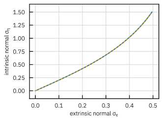
Figure 14: Relation between the standard deviations $\sigma_{\epsilon}$ and $\sigma_{\eta}$ of the extrinsic and intrinsic normal distribution for ellipticity (blue) and a fit by a rational function (dotted orange).

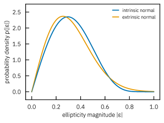
Figure 15: Comparison of intrinsic normal and extrinsic normal ellipticity distributions with standard deviation $\sigma_{\epsilon}=0.256$ in each component.

The change of variable (96) yields the probability distribution function $p$ of the ellipticity magnitude $|\epsilon|$ under the intrinsic normal distribution,

$$p(|\epsilon|)=\frac{4\,\mathrm{e}^{-\frac{2\operatorname{atanh}^{2}|\epsilon|}{\sigma_{\eta}^{2}}}\operatorname{atanh}|\epsilon|}{\sigma_{\eta}^{2}\,(1-|\epsilon|^{2})}\;.$$ (98)

In particular, the resulting standard deviation $\sigma_{\epsilon}$ for a given $\sigma_{\eta}$ can be computed using (98), which yields the relation shown in Figure 15. A useful fit to the curve is

$$\sigma_{\eta}^{2}\approx\sigma_{\epsilon}^{2}\,\frac{8+5\,\sigma_{\epsilon}^{2}}{2-4\,\sigma_{\epsilon}^{2}}\;,$$ (99)

which is good enough to match the intrinsic normal galaxy ellipticity distribution to data from a survey. A comparison between the intrinsic normal and extrinsic normal distributions with $\sigma_{\epsilon}=0.256$ is shown in Figure 15. The most notable difference is the more realistic suppression of high ellipticities with $|\epsilon|>0.8$ in the intrinsic normal case.

Besides, there is also a computational advantage: The extrinsic normal distribution requires explicit rejection of ellipticities with $|\epsilon|>1$, and hence repeated sampling, particularly when $\sigma_{\epsilon}^{2}$ is large. The intrinsic normal distribution accepts all samples for any value of the variance $\sigma_{\epsilon}^{2}$. Given the slightly more realistic shape of the distribution, as well as the improved sampling efficiency, we can generally recommend the intrinsic normal distribution for galaxy ellipticities, particularly when their numbers are large.

References

- Abramo et al. (2016) Abramo L. R., Secco L. F., Loureiro A., 2016, MNRAS, 455, 3871
- Abramo et al. (2022) Abramo L. R., Dinarte Ferri J. V., Tashiro I. L., Loureiro A., 2022, J. Cosmology Astropart. Phys, 2022, 073
- Adamek et al. (2016) Adamek J., Daverio D., Durrer R., Kunz M., 2016, J. Cosmology Astropart. Phys, 2016, 053
- Agarwal & Feldman (2011) Agarwal S., Feldman H. A., 2011, MNRAS, 410, 1647
- Agrawal et al. (2017) Agrawal A., Makiya R., Chiang C.-T., Jeong D., Saito S., Komatsu E., 2017, J. Cosmology Astropart. Phys, 2017, 003
- Alpert & Rokhlin (1991) Alpert B. K., Rokhlin V., 1991, SIAM Journal on Scientific and Statistical Computing, 12, 158
- Alsing et al. (2018) Alsing J., Wandelt B., Feeney S., 2018, MNRAS, 477, 2874
- Alsing et al. (2019) Alsing J., Charnock T., Feeney S., Wandelt B., 2019, MNRAS, 488, 4440
- Alsing et al. (2023) Alsing J., Peiris H., Mortlock D., Leja J., Leistedt B., 2023, ApJS, 264, 29
- Amara & Réfrégier (2007) Amara A., Réfrégier A., 2007, MNRAS, 381, 1018
- Amara et al. (2021) Amara A., et al., 2021, The Journal of Open Source Software, 6, 3056
- Angulo & White (2010) Angulo R. E., White S. D. M., 2010, MNRAS, 405, 143
- Angulo et al. (2021) Angulo R. E., Zennaro M., Contreras S., Aricò G., Pellejero-Ibañez M., Stücker J., 2021, MNRAS, 507, 5869
- Aricò et al. (2020) Aricò G., Angulo R. E., Hernández-Monteagudo C., Contreras S., Zennaro M., Pellejero-Ibañez M., Rosas-Guevara Y., 2020, MNRAS, 495, 4800
- Asgari et al. (2021) Asgari M., et al., 2021, A&A, 645, A104
- Astala et al. (2009) Astala K., Iwaniec T., G. M., 2009, Elliptic Partial Differential Equations and Quasiconformal Mappings in the Plane. No. 48 in Princeton Mathematical Series, Princeton University Press, doi:10.1515/9781400830114
- Balaguera-Antolínez et al. (2018) Balaguera-Antolínez A., Bilicki M., Branchini E., Postiglione A., 2018, MNRAS, 476, 1050
- Benitez et al. (2014) Benitez N., et al., 2014, arXiv e-prints, p. arXiv:1403.5237
- Bird et al. (2012) Bird S., Viel M., Haehnelt M. G., 2012, MNRAS, 420, 2551
- Blas et al. (2011) Blas D., Lesgourgues J., Tram T., 2011, J. Cosmology Astropart. Phys, 2011, 034
- Böhm et al. (2017) Böhm V., Hilbert S., Greiner M., Enßlin T. A., 2017, Phys. Rev. D, 96, 123510
- Boruah et al. (2022) Boruah S. S., Rozo E., Fiedorowicz P., 2022, MNRAS, 516, 4111
- Bose et al. (2021) Bose B., et al., 2021, MNRAS, 508, 2479
- Boyle (2016) Boyle M., 2016, Journal of Mathematical Physics, 57, 092504
- Bridle & King (2007) Bridle S., King L., 2007, New Journal of Physics, 9, 444
- Camacho et al. (2022) Camacho H., et al., 2022, MNRAS, 516, 5799
- Cannon et al. (1997) Cannon J. W., Floyd W. J., Kenyon R., Parry W. R., 1997, in MSRI Publications, Vol. 31, Flavors of Geometry. Cambridge University Press, pp 59–115
- Carrilho et al. (2022) Carrilho P., Carrion K., Bose B., Pourtsidou A., Hidalgo J. C., Lombriser L., Baldi M., 2022, MNRAS, 512, 3691
- Cataneo et al. (2019) Cataneo M., Lombriser L., Heymans C., Mead A. J., Barreira A., Bose S., Li B., 2019, MNRAS, 488, 2121
- Catelan et al. (2001) Catelan P., Kamionkowski M., Blandford R. D., 2001, MNRAS, 320, L7
- Chisari et al. (2015) Chisari N., et al., 2015, MNRAS, 454, 2736
- Chisari et al. (2019) Chisari N. E., et al., 2019, ApJS, 242, 2
- Clerkin et al. (2017) Clerkin L., et al., 2017, MNRAS, 466, 1444
- Coles & Jones (1991) Coles P., Jones B., 1991, MNRAS, 248, 1
- Cordero et al. (2022) Cordero J. P., et al., 2022, MNRAS, 511, 2170
- Cranmer et al. (2020) Cranmer K., Brehmer J., Louppe G., 2020, Proceedings of the National Academy of Science, 117, 30055
- Davé et al. (2019) Davé R., Anglés-Alcázar D., Narayanan D., Li Q., Rafieferantsoa M. H., Appleby S., 2019, MNRAS, 486, 2827
- DeRose et al. (2019) DeRose J., et al., 2019, arXiv e-prints, p. arXiv:1901.02401
- Deshpande et al. (2020) Deshpande A. C., et al., 2020, A&A, 636, A95
- Desjacques et al. (2018) Desjacques V., Jeong D., Schmidt F., 2018, Phys. Rep., 733, 1
- Doré et al. (2014) Doré O., et al., 2014, arXiv e-prints, p. arXiv:1412.4872
- Driscoll & Healy (1994) Driscoll J. R., Healy D. M., 1994, Advances in Applied Mathematics, 15, 202
- Euclid Collaboration et al. (2019) Euclid Collaboration et al., 2019, MNRAS, 484, 5509
- Euclid Collaboration et al. (2020) Euclid Collaboration et al., 2020, A&A, 644, A31
- Fosalba et al. (2008) Fosalba P., Gaztañaga E., Castander F. J., Manera M., 2008, MNRAS, 391, 435
- Fosalba et al. (2015) Fosalba P., Crocce M., Gaztañaga E., Castander F. J., 2015, MNRAS, 448, 2987
- Gatti et al. (2020) Gatti M., et al., 2020, MNRAS, 498, 4060
- Giblin et al. (2019) Giblin B., Cataneo M., Moews B., Heymans C., 2019, MNRAS, 490, 4826
- Giocoli et al. (2010) Giocoli C., Bartelmann M., Sheth R. K., Cacciato M., 2010, MNRAS, 408, 300
- Giocoli et al. (2017) Giocoli C., et al., 2017, MNRAS, 470, 3574
- Górski et al. (2005) Górski K. M., Hivon E., Banday A. J., Wandelt B. D., Hansen F. K., Reinecke M., Bartelmann M., 2005, ApJ, 622, 759
- Graham et al. (2018) Graham M. L., Connolly A. J., Ivezić Ž., Schmidt S. J., Jones R. L., Jurić M., Daniel S. F., Yoachim P., 2018, AJ, 155, 1
- Gruen et al. (2018) Gruen D., et al., 2018, Phys. Rev. D, 98, 023507
- Hall & Taylor (2022) Hall A., Taylor A., 2022, Phys. Rev. D, 105, 123527
- Harnois-Déraps et al. (2018) Harnois-Déraps J., et al., 2018, MNRAS, 481, 1337
- Harris et al. (2020) Harris C. R., et al., 2020, Nature, 585, 357
- Healy et al. (2003) Healy D. M., Rockmore D. N., Kostelec P. J., Moore S., 2003, Journal of Fourier Analysis and Applications, 9, 341
- Heavens et al. (2000) Heavens A., Refregier A., Heymans C., 2000, MNRAS, 319, 649
- Herbel et al. (2017) Herbel J., Kacprzak T., Amara A., Refregier A., Bruderer C., Nicola A., 2017, J. Cosmology Astropart. Phys, 2017, 035
- Heymans & Heavens (2003) Heymans C., Heavens A., 2003, MNRAS, 339, 711
- Heymans et al. (2004) Heymans C., Brown M., Heavens A., Meisenheimer K., Taylor A., Wolf C., 2004, MNRAS, 347, 895
- Hikage et al. (2019) Hikage C., et al., 2019, PASJ, 71, 43
- Hilbert et al. (2011) Hilbert S., Hartlap J., Schneider P., 2011, A&A, 536, A85
- Hildebrandt et al. (2021) Hildebrandt H., et al., 2021, A&A, 647, A124
- Hirata & Seljak (2004) Hirata C. M., Seljak U., 2004, Phys. Rev. D, 70, 063526
- Hoffmann et al. (2022) Hoffmann K., et al., 2022, Phys. Rev. D, 106, 123510
- Hopkins et al. (2018) Hopkins P. F., et al., 2018, MNRAS, 480, 800
- Hopkins et al. (2023) Hopkins P. F., et al., 2023, MNRAS, 519, 3154
- Howlett et al. (2015) Howlett C., Manera M., Percival W. J., 2015, Astronomy and Computing, 12, 109
- Hunter (2007) Hunter J. D., 2007, Computing in Science and Engineering, 9, 90
- Huppenkothen & Bachetti (2022) Huppenkothen D., Bachetti M., 2022, MNRAS, 511, 5689
- Jeffrey & Wandelt (2020) Jeffrey N., Wandelt B. D., 2020, Third Workshop on Machine Learning and the Physical Sciences, NeurIPS 2020, p. arXiv:2011.05991
- Jeffrey et al. (2021) Jeffrey N., Alsing J., Lanusse F., 2021, MNRAS, 501, 954
- Joachimi et al. (2013) Joachimi B., Semboloni E., Hilbert S., Bett P. E., Hartlap J., Hoekstra H., Schneider P., 2013, MNRAS, 436, 819
- Joachimi et al. (2015) Joachimi B., et al., 2015, Space Sci. Rev., 193, 1
- Joachimi et al. (2021) Joachimi B., et al., 2021, A&A, 646, A129
- Jung et al. (2022) Jung G., et al., 2022, ApJ, 940, 71
- Kacprzak et al. (2020) Kacprzak T., et al., 2020, Phys. Rev. D, 101, 082003
- Kacprzak et al. (2023) Kacprzak T., Fluri J., Schneider A., Refregier A., Stadel J., 2023, J. Cosmology Astropart. Phys, 2023, 050
- Kaiser (1998) Kaiser N., 1998, ApJ, 498, 26
- Kayo et al. (2001) Kayo I., Taruya A., Suto Y., 2001, ApJ, 561, 22
- Kiessling et al. (2015) Kiessling A., et al., 2015, Space Sci. Rev., 193, 67
- King & Schneider (2002) King L., Schneider P., 2002, A&A, 396, 411
- Kirk et al. (2015) Kirk D., et al., 2015, Space Sci. Rev., 193, 139
- Kitaura et al. (2016) Kitaura F.-S., et al., 2016, MNRAS, 456, 4156
- Kodi Ramanah et al. (2021) Kodi Ramanah D., Wojtak R., Arendse N., 2021, MNRAS, 501, 4080
- Krause & Hirata (2010) Krause E., Hirata C. M., 2010, A&A, 523, A28
- LSST Science Collaboration et al. (2009) LSST Science Collaboration et al., 2009, arXiv e-prints, p. arXiv:0912.0201
- Laureijs et al. (2011) Laureijs R., et al., 2011, arXiv e-prints, p. arXiv:1110.3193
- Leclercq (2018) Leclercq F., 2018, Phys. Rev. D, 98, 063511
- Lemos et al. (2023) Lemos P., Cranmer M., Abidi M., Hahn C., Eickenberg M., Massara E., Yallup D., Ho S., 2023, Machine Learning: Science and Technology, 4, 01LT01
- Lesgourgues (2011) Lesgourgues J., 2011, arXiv e-prints, p. arXiv:1104.2932
- Levi et al. (2019) Levi M., et al., 2019, in Bulletin of the American Astronomical Society. p. 57 (arXiv:1907.10688)
- Lewis & Bridle (2002) Lewis A., Bridle S., 2002, Phys. Rev. D, 66, 103511
- Lewis et al. (2000) Lewis A., Challinor A., Lasenby A., 2000, ApJ, 538, 473
- Limber (1953) Limber D. N., 1953, ApJ, 117, 134
- Loureiro et al. (2019) Loureiro A., et al., 2019, MNRAS, 485, 326
- Loureiro et al. (2022) Loureiro A., et al., 2022, A&A, 665, A56
- Mead et al. (2021) Mead A. J., Brieden S., Tröster T., Heymans C., 2021, MNRAS, 502, 1401
- Oliveira Franco et al. (2022) Oliveira Franco F., Hadzhiyska B., Alonso D., 2022, arXiv e-prints, p. arXiv:2206.11005
- Padilla & Strauss (2008) Padilla N. D., Strauss M. A., 2008, MNRAS, 388, 1321
- Peacock & Dodds (1996) Peacock J. A., Dodds S. J., 1996, MNRAS, 280, L19
- Pennec (2006) Pennec X., 2006, Journal of Mathematical Imaging and Vision, 25, 127
- Petkova et al. (2014) Petkova M., Metcalf R. B., Giocoli C., 2014, MNRAS, 445, 1954
- Petri et al. (2017) Petri A., Haiman Z., May M., 2017, Phys. Rev. D, 95, 123503
- Pillepich et al. (2018) Pillepich A., et al., 2018, MNRAS, 473, 4077
- Piras et al. (2023) Piras D., Joachimi B., Villaescusa-Navarro F., 2023, MNRAS, 520, 668
- Ramírez-Pérez et al. (2022) Ramírez-Pérez C., Sanchez J., Alonso D., Font-Ribera A., 2022, J. Cosmology Astropart. Phys, 2022, 002
- Refregier & Amara (2014) Refregier A., Amara A., 2014, Physics of the Dark Universe, 3, 1
- Ryden (2004) Ryden B. S., 2004, ApJ, 601, 214
- Schneider (2016) Schneider P., 2016, A&A, 592, L6
- Schneider (2019) Schneider P., 2019, A&A, 624, A54
- Schneider & Teyssier (2015) Schneider A., Teyssier R., 2015, J. Cosmology Astropart. Phys, 2015, 049
- Schneider et al. (2006) Schneider P., Kochanek C. S., Wambsganss J., 2006, Gravitational Lensing: Strong, Weak and Micro. Saas-Fee Advanced Course 33, Springer (arXiv:astro-ph/0407232)
- Schneider et al. (2019) Schneider A., Teyssier R., Stadel J., Chisari N. E., Le Brun A. M. C., Amara A., Refregier A., 2019, J. Cosmology Astropart. Phys, 2019, 020
- Seitz & Schneider (1997) Seitz C., Schneider P., 1997, A&A, 318, 687
- Shields et al. (2011) Shields M., Deodatis G., Bocchini P., 2011, Probabilistic Engineering Mechanics, 26, 511
- Simon (2007) Simon P., 2007, A&A, 473, 711
- Smail et al. (1994) Smail I., Ellis R. S., Fitchett M. J., 1994, MNRAS, 270, 245
- Spergel et al. (2015) Spergel D., et al., 2015, arXiv e-prints, p. arXiv:1503.03757
- Springel et al. (2005) Springel V., et al., 2005, Nature, 435, 629
- Square Kilometre Array Cosmology Science Working Group et al. (2020) Square Kilometre Array Cosmology Science Working Group et al., 2020, PASA, 37, e007
- Sudek et al. (2022) Sudek P., de la Bella L. F., Amara A., Hartley W. G., 2022, MNRAS, 516, 1670
- Takahashi et al. (2012) Takahashi R., Sato M., Nishimichi T., Taruya A., Oguri M., 2012, ApJ, 761, 152
- Takahashi et al. (2017) Takahashi R., Hamana T., Shirasaki M., Namikawa T., Nishimichi T., Osato K., Shiroyama K., 2017, ApJ, 850, 24
- Tanaka et al. (2018) Tanaka M., et al., 2018, PASJ, 70, S9
- Tassev et al. (2013) Tassev S., Zaldarriaga M., Eisenstein D. J., 2013, J. Cosmology Astropart. Phys, 2013, 036
- Taylor et al. (2019) Taylor P. L., Kitching T. D., Alsing J., Wandelt B. D., Feeney S. M., McEwen J. D., 2019, Phys. Rev. D, 100, 023519
- Tortorelli et al. (2020) Tortorelli L., Fagioli M., Herbel J., Amara A., Kacprzak T., Refregier A., 2020, J. Cosmology Astropart. Phys, 2020, 048
- Tosone et al. (2020) Tosone F., Neyrinck M. C., Granett B. R., Guzzo L., Vittorio N., 2020, MNRAS, 498, 2663
- Troxel et al. (2018) Troxel M. A., et al., 2018, Phys. Rev. D, 98, 043528
- Villaescusa-Navarro et al. (2020) Villaescusa-Navarro F., et al., 2020, ApJS, 250, 2
- Voivodic et al. (2019) Voivodic R., Lima M., Abramo L. R., 2019, arXiv e-prints, p. arXiv:1906.06630
- Wei et al. (2018) Wei C., et al., 2018, ApJ, 853, 25
- Xavier et al. (2016) Xavier H. S., Abdalla F. B., Joachimi B., 2016, MNRAS, 459, 3693
- Yoon et al. (2019) Yoon M., Jee M. J., Tyson J. A., Schmidt S., Wittman D., Choi A., 2019, ApJ, 870, 111
- Zonca et al. (2019) Zonca A., Singer L., Lenz D., Reinecke M., Rosset C., Hivon E., Gorski K., 2019, The Journal of Open Source Software, 4, 1298