Efficient optimization of deep neural quantum states toward machine precision

Abstract

Neural quantum states (NQSs) have emerged as a novel promising numerical method to solve the quantum many-body problem. However, it has remained a central challenge to train modern large-scale deep network architectures to desired quantum state accuracy, which would be vital in utilizing the full power of NQSs and making them competitive or superior to conventional numerical approaches. Here, we propose a minimum-step stochastic reconfiguration (MinSR) method that reduces the optimization cost by orders of magnitude while keeping similar accuracy as compared to conventional stochastic reconfiguration. MinSR allows for accurate training on unprecedentedly deep NQS with up to 64 layers and more than $10^{5}$ parameters in the spin-1/2 Heisenberg $J_{1}$-$J_{2}$ models on the square lattice. We find that this approach yields better variational energies as compared to existing numerical results and we further observe that the accuracy of our ground state calculations approaches different levels of machine precision on modern GPU and TPU hardware. The MinSR method opens up the potential to make NQS superior as compared to conventional computational methods with the capability to address yet inaccessible regimes for two-dimensional quantum matter in the future.

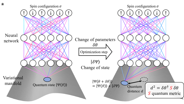
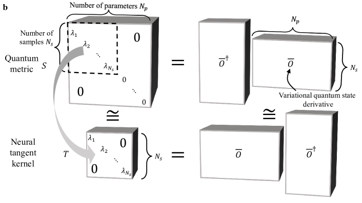
Figure 1: Illustration of neural quantum states (NQS) and minimum-step stochastic reconfiguration (MinSR). a Within the NQS approach an artificial neural network is used to represent a quantum many-body state. A change of the network parameters for an NQS leads to a new quantum state, whose distance to the previous NQS is given by the quantum metric $S\in\mathbb{C}^{N_{p}\times N_{p}}$, where $N_{p}$ is the number of variational parameters. b The quantum metric $S=\overline{O}^{\dagger}\overline{O}$ can be decomposed into a smaller matrix $\overline{O}\in\mathbb{C}^{N_{s}\times N_{p}}$ with $N_{s}\ll N_{p}$ the number of Monte-Carlo samples. The optimization of an NQS involves the inversion of the quantum metric $S$, which is equivalent to determining its nonzero eigenvalues $\lambda_{i}$ with $i=1,\dots,N_{s}$. Within MinSR a neural tangent kernel $T=\overline{O}\,\overline{O}^{\dagger}\in\mathbb{C}^{N_{s}\times N_{S}}$ is introduced with identical eigenvalues $\lambda_{i}$ and therefore the essential information of $S$.

As a fundamental concept in quantum physics, the ground state wave function plays a central role in understanding the behavior of many-body quantum systems. The accurate numerical solution of ground states, however, becomes an extraordinary challenge for existing numerical methods, especially in complex and large two-dimensional systems. The respective challenges depend on the individual utilized method, such as the “curse of dimensionality” in exact diagonalization (ED) [1], the notorious sign problem [2] in quantum Monte Carlo (QMC) [3], or the entanglement growth and matrix contraction complexity in tensor network (TN) methods [4].

Recently, the neural quantum state (NQS) has been introduced as a promising alternative for the calculation of ground states of quantum matter by means of artificial neural networks [5], which has seen already tremendous progress [6, 7, 8, 9]. However, this method also faces an outstanding challenge limiting critically its capabilities and its potential to date. Existing optimization algorithms are not capable of efficiently training modern large-scale deep networks to desired quantum state accuracy in practice, which would be key in order to exploit the full power of this machine learning approach. In this work, we introduce an alternative training algorithm for NQS, which we term the minimum-step stochastic reconfiguration (MinSR). We show that the optimization cost in MinSR is reduced to a leading factor of $N_{p}$ for a deep network with $N_{p}$ parameters, which is a great acceleration compared to conventional stochastic reconfiguration (SR) with $\mathcal{O}(N_{p}^{3})$ complexity or non-parallel iterative solvers. This in turn allows us to train deep neural networks of 64 layers and $10^{5}$ parameters with limited numerical efforts, which is significantly larger than most NQS practice with no more than 10 layers and around $10^{3}$ parameters [5, 10, 8]. We apply our resulting algorithm to paradigmatic two-dimensional quantum spin systems such as the spin-1/2 Heisenberg $J_{1}$-$J_{2}$ model. As a consequence of the now accessible large-scale deep neural networks, we find significantly lower variational energies outperforming conventional numerical approaches up to lattice sizes of $16\times 16$ spins. Most importantly, we observe that our ground state results reach different levels of machine precision. Thus, with MinSR we are able to reach the frontier where the sole limitation of applying the NQS approach to complex two-dimensional quantum matter is not anymore the expressive power of the neural network but rather the inherent numerical precision of the computing device. This is of key importance to exploit the full power of NQS for the calculation of ground states in the future opening up the potential to address yet inaccessible regimes of quantum many-body systems also in higher spatial dimensions.

Neural quantum states

Within the NQS approach, artificial neural networks are utilized to encode the full quantum many-body wave function. In a quantum many-body system with $N$ spin-1/2 degrees of freedom, the Hilbert space can be spanned by the $S_{z}$ spin configuration basis $\ket{\sigma}=\ket{\sigma_{1},\dots,\sigma_{N}}$ with $\sigma_{i}=\,\uparrow$ or $\downarrow$. The neural network is constructed such that it maps every $\sigma$ at the input to a wave function amplitude $\psi_{\sigma}(\theta)$ at the output, for an illustration see Fig. 1. Here, $\theta$ denotes the parameters of the network, i.e., its weights and biases. Hence, the Hilbert space, which is exponentially large in the number of degrees of freedom, is compressed into a much smaller variational space of the network parameters by constructing many-body quantum wave functions via $\ket{\Psi(\theta)}=\sum_{\sigma}\psi_{\sigma}(\theta)\ket{\sigma}$. In order to obtain the variational parameters $\theta$ for the best representation of the ground state of a Hamiltonian $\mathcal{H}$, an NQS is optimized by means of a variational Monte Carlo (VMC) approach [11]. Similar to general machine learning tasks minimizing loss functions, in VMC ground states of quantum systems are obtained by minimizing the variational energy

$$E(\theta)=\frac{\braket{\Psi(\theta)}{\mathcal{H}}{\Psi(\theta)}}{\braket{\Psi(\theta)}{\Psi(\theta)}}$$ (1)

for the target Hamiltonian $\mathcal{H}$. Such minimization procedure for the variational energy is a generic approach in quantum physics and has been utilized extensively also for other choices of variational wave functions with VMC, such as the famous Gutzwiller-projected fermionic wave function (GWF) [11, 12]. However, it is important to emphasize the key difference that traditional wave functions are inspired by specific physical backgrounds and therefore biased due to several reasons such as mean field pictures. As a consequence, they are not guaranteed to asymptotically represent exact wave functions upon increasing the ansatz complexity. The fundamental advantage of NQS on the other hand is that it represents, in principle, a numerically exact algorithm. As guaranteed by the universal approximation theorem [13] and observed empirically by numerous applications of deep learning [14], an NQS is expected to converge to the desired solution to arbitrary accuracy upon increasing the size and depth of the underlying neural network [15].

Current dilemma

As compared to ordinary deep learning tasks in computer science, a major difficulty in NQS is that the rugged quantum landscape [16] with many saddle points imposes a great challenge to the conventional stochastic gradient descent (SGD) method [17]. To improve the optimization dynamics, it is typically necessary to utilize a quantum generalization of natural gradient descent [18] named stochastic reconfiguration (SR) [19]. This increase in precision comes, however, at a significant cost: SR faces a $\mathcal{O}(N_{p}^{3})$ complexity for a neural network with $N_{p}$ parameters, which is much larger than the $\mathcal{O}(N_{p})$ complexity in SGD. Although iterative linear solvers can be employed [5] to reduce the complexity, the time cost is still huge due to the large amount of non-parallel iterations. Consequently, the current applications of NQS mainly focus on shallow networks such as the restricted Boltzmann machine (RBM) [5, 20] or small-scale convolutional neural networks (CNNs) [10, 8]. Although these shallow networks work well in some specific models without sign problem, they also face their natural limitations against TN or GWF in more complex frustrated models, which are of strong current interest, for instance, due to the possibility of realizing celebrated quantum spin liquid phases [21, 22].

Many efforts have been made to overcome the optimization difficulty in deep NQS. For example, simple optimizers including SGD and Adam [23] are used instead of SR at the cost of losing accuracy [24, 25, 26, 27]. While keeping to use SR for high accuracy, large-scale supercomputers are employed to enlarge the allowed number of parameters by a few orders of magnitudes [28, 29], thus compensating the training complexity by computing power. Furthermore, a sequential local optimization approach has also been proposed in which SR only optimizes a portion of all parameters to reduce the time cost [30]. In all these studies, however, the $\mathcal{O}(N_{p}^{3})$ complexity or the non-parallelizable iterative solvers of SR still remain to represent the key limitation for further increasing the network sizes.

Results

Minimum-step stochastic reconfiguration

The central idea of SR is to approximate imaginary-time evolution on the variational state $\ket{\Psi(\theta)}$ in every training step so that the new state $\ket{\Psi^{\prime}}=e^{-\mathcal{H}\delta\tau}\ket{\Psi(\theta)}$ has reduced contributions from eigenstates with higher energies after an imaginary-time interval $\delta\tau$, thereby pushing the state towards the ground state step by step. However, as the variational manifold usually only takes up a tiny portion of the whole Hilbert space, one has to project $\ket{\Psi^{\prime}}$ onto the variational manifold to obtain $\ket{\Psi(\theta^{\prime})}$ with new parameters $\theta^{\prime}$. A common choice of projection is to minimize the difference of the two states given by the Fubini–Study (FS) distance $d(\Psi(\theta^{\prime}),\Psi^{\prime})$ [31, 32, 33]. Expanded to the lowest order of the optimization step $\delta\theta_{k}=\theta^{\prime}_{k}-\theta_{k}$ and the imaginary-time interval $\delta\tau$, we find, as proved in Methods, that $d^{2}(\Psi(\theta^{\prime}),\Psi^{\prime})=N_{s}\sum_{\sigma}\frac{|\psi_{\sigma}|^{2}}{||\Psi||^{2}}\left|\sum_{k}\overline{O}_{\sigma k}\delta\theta_{k}-\overline{\epsilon}_{\sigma}\right|^{2}$, where $N_{s}$ is the number of Monte-Carlo samples to be generated, and $||\Psi||^{2}=\sum_{\sigma}|\psi_{\sigma}|^{2}$. We also adopt the following notations: $\overline{O}_{\sigma k}=(O_{\sigma k}-\braket{O_{\sigma k}})/\sqrt{N_{s}}$ with $O_{\sigma k}=\frac{1}{\psi_{\sigma}}\frac{\partial\psi_{\sigma}}{\partial\theta_{k}}$, $\overline{\epsilon}_{\sigma}=-\delta\tau(E_{\mathrm{loc},\sigma}-\braket{E_{\mathrm{loc},\sigma}})/\sqrt{N_{s}}$ with local energy $E_{\mathrm{loc},\sigma}=\sum_{\sigma^{\prime}}\frac{{\psi_{\sigma^{\prime}}}}{\psi_{\sigma}}H_{\sigma{\sigma^{\prime}}}$, and $\braket{...}=\sum_{\sigma}\frac{|\psi_{\sigma}|^{2}}{||\Psi||^{2}}...$ is the expectation value. The quantum metric expression can be evaluated by Monte-Carlo samples as

$$d^{2}(\Psi(\theta^{\prime}),\Psi^{\prime})=\sum_{\sigma\mathrm{\,in\,samples}}\left|\sum_{k}\overline{O}_{\sigma k}\delta\theta_{k}-\overline{\epsilon}_{\sigma}\right|^{2},$$ (2)

where the sum of spin configuration $\sigma$ is performed over $N_{s}$ Monte-Carlo samples taken from the probability distribution $|\psi_{\sigma}(\theta)|^{2}/||\Psi(\theta)||^{2}$. Eq. (2) can be reformulated as $d(\Psi(\theta^{\prime}),\Psi^{\prime})=||\overline{O}\delta\theta-\overline{\epsilon}||$ if we treat $\delta\theta$ and $\overline{\epsilon}$ as vectors and $\overline{O}$ as a matrix. As a key consequence, we introduce a new linear equation

$$\overline{O}\delta\theta=\overline{\epsilon}\,,$$ (3)

whose least-squares solution minimizes the FS distance and leads to the SR equation. Conceptually, one can understand the left-hand side of this equation as the change of the variational state induced by an optimization step of the parameters, and the right-hand side as the change of the exact imaginary-time evolving state. The SR solution minimizing their difference is given by

$$\delta\theta=S^{-1}\overline{O}^{\dagger}\overline{\epsilon}\quad\mathrm{with}\,S=\overline{O}^{\dagger}\overline{O}.$$ (4)

In most literature [5, 19], Eq. (4) is directly shown as a solution minimizing the FS distance, but here we show that it can also be derived as the least-squares solution of Eq. (3) which will lead to natural and key improvements as we will discuss in detail later.

As illustrated in Fig. 1, the matrix $S$ in Eq. (4) plays an important role as the quantum metric in VMC, i. e., the FS distance is $d^{2}(\Psi(\theta),\Psi(\theta^{\prime}))=\delta\theta^{\dagger}S\,\delta\theta$ for states before and after a variation of parameters $\delta\theta$ [18, 33]. A major difficulty of SR is the computation of $S^{-1}$ which helps to map a variation in the Hilbert space back to the parameter space. For an optimization step with $N_{s}$ samples and $N_{p}$ parameters, the shapes of $\overline{O}$ and $S$ are $N_{s}\times N_{p}$ and $N_{p}\times N_{p}$ respectively, and the complexity of solving Eq. (4) is hence $\mathcal{O}(N_{p}^{2}N_{s}+N_{p}^{3})$ for direct linear solvers and becomes unacceptable for deep networks. Many iterative methods including conjugate gradient (cg) and minres [34] can be employed to reduce the complexity of SR to $\mathcal{O}(N_{p}N_{s}N_{\mathrm{iter}})$ [35], where $N_{\mathrm{iter}}$ is the number of iterations in the iterative solver. However, with large $N_{s}$ and $N_{p}$ the iterative approach is typically facing natural limitations by a huge required $N_{\mathrm{iter}}$ and non-parallelizable iterations. In Ref. [28, 29] with $N_{p}\sim 10^{5}$ and $N_{s}\sim 10^{6}$, for instance, the direct linear solver is still adopted instead of iterative solvers.

To reduce the cost of SR, we focus on a specific optimization case of a deep network with a large number of parameters $N_{p}$ but a relatively small amount of batch samples $N_{s}$ similar to most deep learning research. We assume, and justify below, that NQS can still converge to the minimum energy even with reduced $N_{s}$ and lower optimization accuracy caused, and the expressive power controlled by $N_{p}$ is the dominant factor affecting the final variational accuracy. In this case, as shown in Fig. 1, the rank of the $N_{p}\times N_{p}$ matrix $S=\overline{O}^{\dagger}\overline{O}$ is at most $N_{s}$, meaning that $S$ contains much less information than its capacity due to an insufficient number of batch samples. As a more efficient way to express the information of the quantum metric, we introduce the neural tangent kernel $T=\overline{O}\,\overline{O}^{\dagger}$ [36] containing the same non-zero eigenvalues as $S$ but reducing the matrix size from $N_{p}\times N_{p}$ to $N_{s}\times N_{s}$.

Here, we propose a new method based on using $T$ as the compressed matrix. To formulate this method, we notice that Eq. (3) is underdetermined with an infinite amount of least-squares solutions when $N_{s}<N_{p}$. To obtain a unique $\delta\theta$ solution, we employ the least-squares minimum-norm condition which is widely used for underdetermined linear equations. To be specific, we choose, among all solutions with minimum residual error $||\overline{O}\delta\theta-\overline{\epsilon}||$, the one minimizing the norm of variational step $||\delta\theta||=\sqrt{\sum_{k}|\delta\theta_{k}|^{2}}$, which helps to reduce higher-order effects, prevent overfitting and improve stability. We name this method minimum-step SR (MinSR) due to the additional minimum-step condition. In Methods we provide two approaches to obtain the following MinSR solution

$$\delta\theta=\overline{O}^{\dagger}T^{-1}\overline{\epsilon}\quad\mathrm{with}\,T=\overline{O}\,\overline{O}^{\dagger},$$ (5)

which only requires the inverse of an $N_{s}\times N_{s}$ matrix with an $\mathcal{O}(N_{p}N_{s}^{2}+N_{s}^{3})$ complexity. For large $N_{p}$, it provides a tremendous acceleration with a time cost proportional to $N_{p}$ instead of $N_{p}^{3}$, and the employment of non-parallel iterative solvers is also avoided. Therefore, it can be viewed as a natural reformulation of traditional SR which is particularly useful in the limit $N_{p}\gg N_{s}$ as relevant in deep learning situations.

It is important to emphasize that, although the reduced number of samples $N_{s}$ in MinSR leads to increased uncertainty of energy when evaluating $\braket{E_{\mathrm{loc},\sigma}}$, it does not have a significant impact on the optimization accuracy. The reason is that the local energies of samples roughly fall into the range $\braket{E_{\mathrm{loc},\sigma}}\pm\mathrm{std}(E_{\mathrm{loc}})$, but the uncertainty of $\braket{E_{\mathrm{loc},\sigma}}$ is only $u(\braket{E_{\mathrm{loc},\sigma}})=\mathrm{std}(E_{\mathrm{loc}})/\sqrt{N_{s}}\ll\mathrm{std}(E_{\mathrm{loc}})$ as long as $N_{s}$ is not too small, so $u(\braket{E_{\mathrm{loc},\sigma}})$ only causes a small error when computing $\overline{\epsilon}_{\sigma}=-\delta\tau(E_{\mathrm{loc},\sigma}-\braket{E_{\mathrm{loc},\sigma}})/\sqrt{N_{s}}$ for MinSR optimization. Similar argument also applies to $\overline{O}_{\sigma k}$. Furthermore, as $\mathrm{std}(E_{\mathrm{loc}})\rightarrow 0$ when the wave function is close to convergence in VMC [11], one can easily obtain a small $u(E)$ without too many samples when evaluating the expectation value of energy, as we will see for the specific numerical benchmark examples studied below. For other observables with finite standard deviations, the large amount of required samples can be generated after training convergence which does not slow down the optimization.

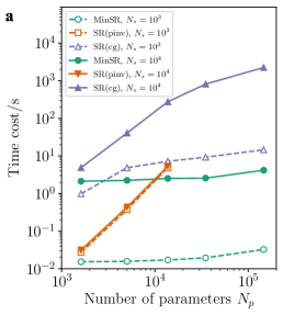
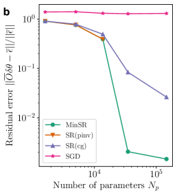
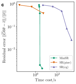
Figure 2: Performance evaluation of various optimization methods in solving the linear equation $\overline{O}\delta\theta=\overline{\epsilon}$ for a single training step. The tested methods include stochastic gradient descent (SGD), stochastic reconfiguration (SR) with both the pseudo-inverse (pinv) and conjugate gradient (cg) solvers as well as minimum-step SR (MinSR). The SR (pinv) result is unavailable for $N_{p}\gtrsim 10^{4}$ due to memory constraints on the utilized A100 80G GPU. a Time cost in seconds for the different optimization methods as a function of the number of variational parameters $N_{p}$ for different numbers of Monte-Carlo samples $N_{s}$. b Relative residual error $||\overline{O}\delta\theta-\overline{\epsilon}||/||\overline{\epsilon}||$ for $N_{s}=10^{4}$. c Relation between the residual error and time cost for $N_{s}=10^{4}$.

Benchmark models

To showcase the performance of MinSR, we apply it to the paradigmatic spin-1/2 Heisenberg $J_{1}$-$J_{2}$ model on the square lattice which serves as a benchmark system in various NQS studies and provides a convenient comparison to other state-of-the-art methods as will be shown in the following. The Hamiltonian of the system is given by

$$\mathcal{H}=J_{1}\sum_{\left<i,j\right>}{\bf{S}}_{i}\cdot{\bf{S}}_{j}+J_{2}\sum_{\left<\left<i,j\right>\right>}{\bf{S}}_{i}\cdot{\bf{S}}_{j},$$ (6)

where ${\bf{S}}_{i}=(S_{i}^{x},S_{i}^{y},S_{i}^{z}$) with $S_{i}^{x},S_{i}^{y},S_{i}^{z}$ spin-1/2 operators at site $i$, $\left<i,j\right>$ and $\left<\left<i,j\right>\right>$ indicate pairs of nearest-neighbor and next-nearest neighbor sites, respectively, and $J_{1}$ is chosen equal to 1 for simplicity in this work.

We will specifically focus on two points in parameter space: $J_{2}/J_{1}=0$ and $J_{2}/J_{1}=1/2$. At $J_{2}/J_{1}=0$, the Hamiltonian reduces to the non-frustrated Heisenberg model. At $J_{2}/J_{1}=1/2$, the $J_{1}$-$J_{2}$ model becomes strongly frustrated close to the maximally frustrated point where the system resides in a quantum spin liquid phase [7], which imposes a great challenge on existing numerical methods including NQS [37, 10].

Performance comparison

We now start with a direct performance comparison among various optimization methods, including SGD, MinSR, and SR with direct pseudo-inverse (pinv) solver or iterative conjugate gradient (cg) solver. Each of these methods involves for each optimization step the inversion of $S$ or $T$ as shown in Eq. (4) and Eq. (5), which is usually ill-conditioned. Thus, it is important to identify a suitable regularization. In our numerical experiments, pseudo-inverse with relative tolerance $r_{\mathrm{tol}}=10^{-12}$ is used for MinSR and SR (pinv). For SR (cg), the diagonal shift $S^{\mathrm{reg}}_{ii}=S_{ii}+\varepsilon_{1}S_{ii}+\varepsilon_{2}$ with $\varepsilon_{1}=10^{-4}$ and $\varepsilon_{2}=0$ is applied. An alternative choice is $\varepsilon_{2}\neq 0$ [9], but in our tests it does not help to improve the performance of SR. In order to demonstrate the overall capability and performance of each of these algorithms, their efficiency and accuracy are tested on the $10\times 10$ Heisenberg model. In each test, an NQS close to convergence is used to generate $\overline{O}$ and $\overline{\epsilon}$ by drawing Monte-Carlo samples, and different methods are employed to produce approximate solutions of Eq. (3). The whole experiment is performed on a single NVIDIA A100 80GB GPU.

The time cost of each algorithm in solving Eq. (3) is shown in Fig. 2 for a comparison of their efficiency. The test is performed with two batch sizes $N_{s}=10^{3}$ and $10^{4}$, and multiple networks with different amounts of parameters $N_{p}$. SR (cg) searches for solutions with non-parallel iterations, causing much larger time costs compared to other methods. For the test with the largest available $N_{s}$ and $N_{p}$, the time cost of SR (cg) is more than 500 times larger than MinSR and becomes the bottleneck of optimization. On the other hand, the time cost of SR (pinv) is larger than MinSR when $N_{p}>N_{s}$ and grows rapidly with $N_{p}$, which matches our complexity analysis. Furthermore, SR (pinv) is unable to produce any result for $N_{p}\gtrsim 10^{4}$ due to the memory cost of inverting $S$ even on an A100 80GB GPU with the largest available memory currently available for GPUs. In summary, MinSR has a great efficiency advantage in the large $N_{p}$ regime compared to traditional SR. Moreover, MinSR makes it possible to obtain direct pseudo-inverse solutions within the limited memory space provided by modern GPU or TPU, which helps to avoid the usage of massive CPU resources as has been done recently [20, 29, 38] and further reduces the time cost.

To compare the accuracy of different methods, in Fig. 2 we evaluate the relative residual error $r=||\overline{O}\delta\theta-\overline{\epsilon}||/||\overline{\epsilon}||$ similar to the one employed in Ref. [5, 39]. The SGD error is larger than 1, meaning that the direct energy gradient direction does not coincide with the imaginary-time evolution direction given by SR and is unlikely to further optimize the variational wave function when the NQS is close to convergence. The SR (cg) method produces biased solutions due to the diagonal shift of $S$, while the pseudo-inverse method provides a strict cut-off to small eigenvalues and minimizes the residual error under given regularization. When $N_{p}>N_{s}=10^{4}$, especially, the matrix $S$ in SR contains a lot of vanishing eigenvalues, in which case the SR (cg) method exhibits a much worse accuracy compared to MinSR or SR (pinv). Moreover, the MinSR and SR (pinv) methods, as explained in Methods, give the same solution up to numerical precision, but MinSR makes it possible to apply a very accurate pseudo-inverse solution to larger networks with more parameters.

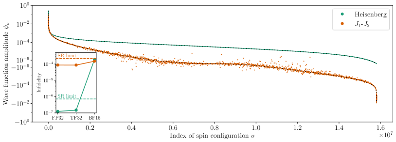
Figure 3: Neural quantum state (NQS) wave function amplitudes for the Heisenberg and $J_{1}$-$J_{2}$ models on a $6\times 6$ square lattice obtained by deep convolutional neural networks (CNNs) with 64 layers and 146320 parameters by means of minimum-step stochastic reconfiguration (MinSR). The spin configurations are sorted according to the exact diagonalization (ED) wave function amplitudes in descending order as shown by the black dotted lines. All wave function amplitudes are shown for the Heisenberg model, while for the $J_{1}$-$J_{2}$ model only one point is plotted among 10000 successive points. In the inset, we show the infidelity obtained by the deep CNN with different numerical precision. The infidelity of a medium-scale CNN with 13750 parameters which approaches the size limit of SR (pinv) is also presented for comparison.

In Fig. 2 we plot the change of residual error as deeper networks with larger time costs are employed. The same data as Fig. 2 and Fig. 2 is used. The MinSR method is able to produce accurate results by using deeper networks without significantly longer time costs, providing a reliable approach for accurate solutions in VMC which helps the optimization to converge faster. On the contrary, one has to spend much more time obtaining accurate solutions if traditional SR is adopted. In summary, MinSR drastically outperforms the traditional SR method in that it requires orders of magnitude less time costs without loss of accuracy. It brings accurate SR optimization to a next level for deep NQS, which makes it possible to train variational wave functions even toward machine precision for exact ground states of quantum matter.

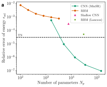
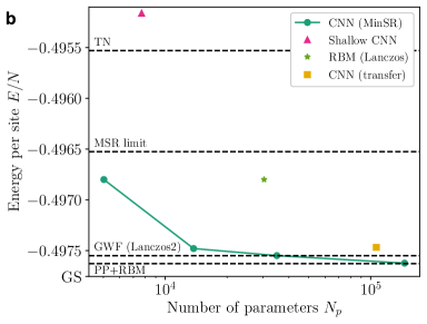
Figure 4: Variational ground-state energies $E$ for the $10\times 10$ square lattice. a Relative error of the variational ground-state (GS) energy $\epsilon_{\mathrm{rel}}=(E-E_{\mathrm{GS}})/|E_{\mathrm{GS}}|$, with $E_{\mathrm{GS}}$ being the ground-state energy, for the non-frustrated Heisenberg model as a function of the number of variational parameters $N_{p}$. The variational energies obtained in this work by means of a deep convolutional neural network (CNN) trained with the minimum-step stochastic configuration (MinSR) are compared to previous results in the literature including restricted Boltzmann machines (RBMs) [5], shallow CNNs [10], and RBMs with an additional exact Lanczos step [38]. As no tensor network (TN) data is available in the periodic boundary condition (PBC), the best result with an open boundary condition (OBC) is included as a dashed line [40], b Ground-state energies of the frustrated $J_{1}$-$J_{2}$ model at $J_{2}/J_{1}=0.5$. The results by means of MinSR obtained in this work for a CNN are compared to previous results in the literature for shallow CNN [10], RBM with an additional exact Lanczos step [38], and CNN with transfer learning [29]. Further results from methods other than NQS are included as dashed lines such as TN [41], the Gutzwiller wave function (GWF) with 2 additional exact Lanczos steps (Lanczos2) [42], and the combination of pair product state (PP) and RBM [7]. The exact GS energy in the frustrated case is estimated by extrapolation of variational energy and energy variance in our NQS results. As a further reference, the so-called Marshall sign rule (MSR) limit is included, which is obtained from an NQS training for a wave function where the sign structure is not learned but rather fixed by the MSR.

Optimization results

Having demonstrated the superior performance of MinSR in terms of runtime and accuracy as compared to other optimization algorithms, it is the goal in the following to apply MinSR to paradigmatic physical problems. In particular, it will be the purpose to benchmark our MinSR results against existing results in the literature with the goal of demonstrating that our introduced approach of utilizing NQS in combination with MinSR allows us to outperform existing methods. The VMC optimization is performed on deep networks with up to 64 layers and 146320 parameters, which is larger than all previous networks trained by SR to convergence until now.

In a first step we aim to show the accuracies obtainable with our introduced method on the level of the full quantum many-body wave function. For that purpose we display in Fig. 3 full NQS wave functions obtained on the $6\times 6$ Heisenberg $J_{1}$-$J_{2}$ model. The ED results obtained by the lattice-symmetries package [43] are shown as dotted lines for reference. The full wave functions are given in the ground state sector with a Hilbert-space dimension of 15804956, which is much larger than the number of network parameters and therefore still presents a challenge to the expressive power of NQS. The NQS wave function exhibits a nearly exact match with the ED result in the non-frustrated case without any obvious outliers among more than $10^{7}$ components, showing the outstanding performance of deep NQS in expressing non-frustrated wave functions upon utilizing MinSR, which makes the training possible for such huge networks. In the frustrated case, one can observe a slightly different behavior. The deep network is still capable of accurately capturing the dominant wave function amplitudes $\psi_{\sigma}$, while deviations start to appear on a scale of the order of $10^{-5}$. Notice that in terms of probabilities $|\psi_{\sigma}|^{2}$ this implies errors to appear only on the level of $10^{-10}$ or even smaller. Further, the dominant challenge for the NQS wave function is still to learn proper sign structures, as the wave function amplitudes of small magnitude often do not have correct signs. Nevertheless, the full wave function is still very accurate because those inaccurate components are all very close to zero with marginal effects on the overall quantum state. In order to quantify the accuracy of how well the deep NQS has learned the sign structure we calculate a sign structure error defined as

$$e_{s}=\sum_{\begin{subarray}{c}\sigma\\ \mathrm{sgn}(\psi_{\sigma})\neq\mathrm{sgn}(\phi_{\sigma})\end{subarray}}|\phi_{\sigma}|^{2},$$ (7)

where $\psi_{\sigma}$ and $\phi_{\sigma}$ are variational and exact wave function amplitudes, respectively. This error is expected to vanish a completely accurate sign structure and $1/2$ for a random one. If NQS does not learn any frustrated behavior and only gives the so-called Marshall sign rule (MSR) [44], the error is $e_{s}=0.020$. The well-trained deep NQS in our work presents a further correction to MSR and gives $e_{s}=1.3\times 10^{-6}$, showing extraordinary performance in learning the frustrated sign structure.

Having outlined the achieved excellent accuracies for the wave function amplitudes, we now aim to go one step further by demonstrating that our approach is actually capable to reach a fundamental and long-sought goal of NQS: Upon increasing the size of the neural network the NQS solution is supposed to converge to the exact one, so that the sole limitation of NQS becomes the numerical precision of the computing device. For that purpose, we also compute the wave function amplitudes when different precision, including 32-bit floating-point (FP32), TensorFloat-32 (TF32), and bfloat16 (BF16), is employed for evaluating the NQS wave function. In the inset of Fig. 3 we show the infidelity defined as

$$1-\frac{\braket{\Psi}{\Phi}\braket{\Phi}{\Psi}}{\braket{\Psi}{\Psi}\braket{\Phi}{\Phi}},$$ (8)

where $\Psi$ and $\Phi$ are the variational and exact ground states, respectively. In the non-frustrated Heisenberg model, the nearly vanishing infidelity implies an almost perfect match between the variational state and the exact ground state. The infidelity increases slightly on TF32 and dramatically on BF16, indicating that the accuracy of the obtained wave function approaches the limit of TF32. We also compute the infidelity limit, which is $4.5\times 10^{-8}$, when $\psi_{\sigma}$ and $\phi_{\sigma}$ are respectively given by the ground state wave function with 16-bit floating-point (FP16) and FP32. As FP16 and TF32 give similar accuracy, we notice that our variational infidelity $1.2\times 10^{-7}$ is only 2.6 times larger than the limit of TF32. Considering the error accumulation in the forward pass of the deep network, this result has well approached the TF32 machine precision. In the frustrated $J_{1}$-$J_{2}$ model, the infidelity is roughly unchanged from FP32 to TF32, but obviously increases from TF32 to BF16, which means the deep NQS trained by MinSR approaches BF16 precision. Another piece of evidence is that the BF16 result in the Heisenberg model roughly indicates the precision limit of BF16 and the result in the $J_{1}$-$J_{2}$ model gets below this level. Although many small wave-function components exhibit deviations as shown by the full $J_{1}$-$J_{2}$ wave function, the infidelity under BF16 precision is still mainly caused by the reduced precision of large components. Furthermore, we also present the infidelity obtained by a CNN with 13750 parameters, which, as shown in Fig. 2, is roughly the maximum network size allowed for SR (pinv) on GPU. As shown in the inset of Fig. 3, the conventional SR method is unable to approach machine precision because its infidelity is limited to a level far above MinSR. In conclusion, the deep network architecture with the help of MinSR plays a critical role in pushing the NQS accuracy toward machine precision.

After quantifying the accuracy of our approach for small systems upon comparing to ED, it will be the key goal in the following to show that the deep networks trainable now by MinSR lead to a numerical algorithm that outperforms existing methods for large system sizes beyond the reach of ED, in particular for the considered Heisenberg $J_{1}$-$J_{2}$ model. First, we start by focusing on systems with a $10\times 10$ lattice. In this case, the huge Hilbert space becomes a greater challenge for the expressive power and the generalization ability of NQS compared with the $6\times 6$ lattice. As the benchmarks of NQS are mostly given in the $10\times 10$ lattice, it also provides the ideal starting point to compare our introduced scheme with the performance of other methods. In each optimization attempt, 20000 training steps are performed without symmetry, followed by 10000 steps with imposed symmetry as shown by Eq. (38) in Methods, and the number of samples $N_{s}$ is fixed at 10000.

In the non-frustrated Heisenberg model, the deep NQS trained by MinSR provides an unprecedentedly precise result better than all existing variational methods as shown in Fig. 4. The adopted reference ground-state energy per site is $E_{\mathrm{GS}}/N=-0.67155267(5)$, as given by a stochastic series expansion (SSE) [45] simulation performed by ourselves, instead of the commonly used reference $E/N=-0.671549(4)$ from Ref. [46] because our best NQS variational energy $E/N=-0.67155260(3)$ provides an even better accuracy as compared to this common reference energy. Thanks to the deep network architecture and the efficient MinSR method, the relative error of variational energy $\epsilon_{\mathrm{rel}}=(E-E_{\mathrm{GS}})/|E_{\mathrm{GS}}|$ drops much faster than the 1-layer RBM as $N_{p}$ increases and finally reaches a level of $10^{-7}$. Compared with other variational results, our best variational energy is about $10^{4}$ times more accurate than what has been obtained by means of shallow NQSs including RBM [5] and shallow CNN [10], and still around $10^{3}$ times more accurate than the best NQS result before this work given by an additional exact Lanczos step on RBM [38]. Since autoregressive networks and TN are both known to be more suitable for open boundary conditions (OBCs) instead of periodic boundary conditions (PBCs) used in this work, here for comparison we also give their relative error of variational energy in OBCs, which is $\epsilon_{\mathrm{rel}}=3.5\times 10^{-5}$ [24] and $\epsilon_{\mathrm{rel}}=3.0\times 10^{-5}$ [40], respectively, while in our work the most accurate result gives $\epsilon_{\mathrm{rel}}\approx 10^{-7}$ in PBC. Although OBC and PBC results are not directly comparable, the huge difference in accuracy still hints at a possibly much more accurate variational state. As the autoregressive network in Ref. [24] is also a deep network with around one million parameters but trained by SGD, this comparison also shows that MinSR is indispensable even in the simple non-frustrated case.

In order to go to the next level of complexity we will now focus on the frustrated $J_{1}$-$J_{2}$ model, whose accurate ground-state solution has remained a key challenge for all available computational approaches. As we show in Fig. 4 for a $10\times 10$ lattice, our introduced method based on MinSR allows us to reach ground-state energies below what is possible with other numerical schemes. In this context, the MSR limit shows the energy one can obtain without considering any frustration. As shown in the figure, the usage of deep NQS becomes absolutely crucial as the shallow CNN is not guaranteed to beat the MSR limit. Most importantly, our obtained variational energy is reduced upon increasing the network size and finally outperforms all existing NQS results and arrives at the same level of energy as the best existing result given by the combination of a special kind of GWF named pair product state (PP) and RBM [7]. Although PP+RBM produces similar energy with a smaller number of parameters $N_{p}$ than our deep CNN due to its additional physical input encoded in the GWF, their computational complexity is comparable because some additional computations are required to enforce the translation symmetry in PP+RBM which is unnecessary for the CNN. This result shows that the deep NQS trained by MinSR is superior even in the frustrated case which was argued to be challenging for NQS on a general level [47].

Table 1: Variational ground-state energy per site $E/N$ for the frustrated $J_{1}$-$J_{2}$ model at $J_{2}/J_{1}=0.5$ on the $16\times 16$ square lattice.

Wave function	Reference	$E/N$
PP+RBM	[7]	$-0.496213(3)$
GCNN	[9]	$-0.496407(7)$
CNN(transfer)	[29]	$-0.49659$
CNN(MinSR)	This work	$-0.496683(2)$

Finally, we aim to provide evidence that our approach exhibits an even more advantageous performance as compared to other computational methods upon further increasing system size. In Table 1 the obtained variational energy on a $16\times 16$ square lattice is presented and compared to existing results in the literature. In our training, the variational parameters from the $10\times 10$ lattice are used as the initial parameters through transfer learning [28] to reduce time cost. One can clearly see that our approach yields the best variational energy for the frustrated $J_{1}$-$J_{2}$ model on such a large lattice. In this system, our variational energy is obviously below the PP+RBM [7] and TN [48] energies. Compared with the best existing variational result given in Ref. [29], the energy in this work is still $2\times 10^{-4}$ lower. In summary, the deep NQS trained by MinSR obtains state-of-the-art or even superior results in large frustrated models, which fills the gap in efficient and reliable numerical methods for large two-dimensional quantum matter and might become an indispensable approach for discovering new intriguing quantum many-body phenomena in such complex systems.

Discussion

In this Article, we have introduced an alternative method, termed MinSR, to train NQS wave functions. We have shown that MinSR reduces the time cost of optimization by orders of magnitude for deep NQS as compared to traditional SR methods while maintaining the same level of accuracy. We have demonstrated that MinSR allows us to successfully train deep NQSs with up to 64 layers and more than $10^{5}$ parameters. It is a key outcome of this work that the achieved variational ground-state energies outperform all existing variational results on the considered paradigmatic quantum spin models. In the non-frustrated Heisenberg model on the square lattice, we show that the accuracy of the variational energy is improved by orders of magnitude toward TF32 precision. Further, for the frustrated $J_{1}$-$J_{2}$ model the MinSR approach outperforms the best existing variational results and approaches BF16 precision. Based on our findings we expect that MinSR is the starting point to put the NQS approach for solving the quantum many-body problem on a next level with the potential to address complex quantum matter in previously inaccessible regimes.

We identify many directions along which our current results might be further improved. For instance, MinSR provides an additional condition, in this work chosen as minimizing $||\delta\theta||$ in Eq. (3), to control the variational optimization under the constraint of the minimum residual error $||\overline{O}\delta\theta-\overline{\epsilon}||$. One is free to adopt other conditions for potentially controlling better the training stability or to include higher-order effects in NQS optimization, which may lead to even better variational accuracy. A further improvement of the variational energies of the considered models might be likely achievable by choosing more specific deep neural network architectures with additional physical input.

The CNN architecture is scalable to larger system sizes through transfer learning [28], as we have also shown here, and it is also sufficiently flexible to target various types of lattices [47, 8]. Thus, one can expect that deep CNNs in combination with the MinSR method provide a powerful approach to target quantum matter, which is challenging to solve by other means, with the potential to discover new quantum phenomena, especially concerning complex high-dimensional systems such as the pyrochlore Heisenberg model [49, 8], where TN and GWF do not provide sufficient accuracy.

In this work we have applied MinSR for the variational search of ground-state wave functions. It is important to emphasize, however, that the fundamental Eq. (3), solved by MinSR, can be directly translated to a time-dependent variational principle for solving the dynamics of quantum matter by means of NQS [5, 39]. It is therefore a natural question to which extent the MinSR method might also be applicable to such time-evolution problems in order to yield improved solutions of the fundamental equation of quantum mechanics - the Schrödinger equation.

Moreover, it is key to point out that the MinSR method is not at all restricted to NQS. As a general optimization method in VMC, it can also be applied to other more traditional wave functions like TN or GWF so that more complex ansatz architecture can be introduced in these conventional methods to include more physical insights. We can further envision the application of MinSR beyond the scope of physics for general machine learning tasks in case a suitable space for optimization similar to the Hilbert space in physics can be defined in order to construct an equation similar to Eq. (3).

Methods

Fubini-Study distance

The original definition of the Fubini-Study distance between the variational state $\ket{\Psi(\theta^{\prime})}=\ket{\Psi(\theta+\delta\theta)}$ and the imaginary-time evolving state $\ket{\Psi^{\prime}}=e^{-\mathcal{H}\delta\tau}\ket{\Psi(\theta)}$ is [31, 32, 33]

$$d(\Psi(\theta^{\prime}),\Psi^{\prime})=\arccos\frac{|\braket{\Psi(\theta^{\prime})}{\Psi^{\prime}}|}{||\Psi(\theta^{\prime})||\cdot||\Psi^{\prime}||}.$$ (9)

Assuming that $\ket{\Psi(\theta^{\prime})}=\ket{\Psi}+\ket{\delta\Psi_{\theta}}$ and $\ket{\Psi^{\prime}}=\ket{\Psi}+\ket{\delta\Psi_{H}}$ where $\ket{\delta\Psi_{\theta}}$ and $\ket{\delta\Psi_{H}}$ are both small quantities, one can expand the FS distance to the lowest order of $\ket{\delta\Psi}/||\Psi||$ as

$$d^{2}(\Psi(\theta^{\prime}),\Psi^{\prime})=\left(\bra{\delta\tilde{\Psi}_{\theta}}-\bra{\delta\tilde{\Psi}_{H}}\right)\left(\ket{\delta\tilde{\Psi}_{\theta}}-\ket{\delta\tilde{\Psi}_{H}}\right),$$ (10)

where

$$\ket{\delta\tilde{\Psi}}=\frac{\ket{\delta\Psi}}{||\Psi||}-\frac{\braket{\Psi}{\delta\Psi}\ket{\Psi}}{||\Psi||^{3}}$$ (11)

is the normalized increment perpendicular to the original state for $\ket{\delta\tilde{\Psi}_{\theta}}$ and $\ket{\delta\tilde{\Psi}_{H}}$.

The change of $\ket{\Psi_{\theta}}$ is induced by the change of parameters as

$$\ket{\delta\Psi_{\theta}}=\sum_{\sigma}\sum_{k}\frac{\partial\psi_{\sigma}}{\partial\theta_{k}}\delta\theta_{k}\ket{\sigma}=\sum_{\sigma}\psi_{\sigma}\sum_{k}O_{\sigma k}\delta\theta_{k}\ket{\sigma},$$ (12)

where $O_{\sigma k}=\frac{1}{\psi_{\sigma}}\frac{\partial\psi_{\sigma}}{\partial\theta_{k}}$. According to the imaginary-time evolution $\ket{\Psi^{\prime}}=e^{-\mathcal{H}\delta\tau}\ket{\Psi(\theta)}$, the change of the state $\ket{\Psi^{\prime}}$ to the first order of $\delta\tau$ is

$$\ket{\delta\Psi_{H}}=-\mathcal{H}\delta\tau\ket{\Psi(\theta)}=-\delta\tau\sum_{\sigma}\psi_{\sigma}E_{\mathrm{loc},\sigma}\ket{\sigma},$$ (13)

where $E_{\mathrm{loc},\sigma}=\sum_{\sigma^{\prime}}\frac{{\psi_{\sigma^{\prime}}}}{\psi_{\sigma}}H_{\sigma{\sigma^{\prime}}}$. Putting Eq. (12) and Eq. (13) into Eq. (11), we obtain

$$\ket{\delta\tilde{\Psi}_{\theta}}=\sqrt{N_{s}}\sum_{\sigma}\frac{\psi_{\sigma}}{||\Psi||}\sum_{k}\overline{O}_{\sigma k}\delta\theta_{k}\ket{\sigma},$$ (14)

$$\ket{\delta\tilde{\Psi}_{H}}=\sqrt{N_{s}}\sum_{\sigma}\frac{\psi_{\sigma}}{||\Psi||}\overline{\epsilon}_{\sigma}\ket{\sigma},$$ (15)

where $\overline{O}_{\sigma k}=(O_{\sigma k}-\braket{O_{\sigma k}})/\sqrt{N_{s}}$, $\overline{\epsilon}_{\sigma}=-\delta\tau(E_{\mathrm{loc},\sigma}-\braket{E_{\mathrm{loc},\sigma}})/\sqrt{N_{s}}$.

Substituting Eq. (14) and Eq. (15) into Eq. (10), the FS distance becomes

$$d^{2}(\Psi(\theta^{\prime}),\Psi^{\prime}) =N_{s}\sum_{\sigma}\frac{|\psi_{\sigma}|^{2}}{||\Psi||^{2}}\left|\sum_{k}\overline{O}_{\sigma k}\delta\theta_{k}-\overline{\epsilon}_{\sigma}\right|^{2}$$ (16)

$$=N_{s}\left<\left|\sum_{k}\overline{O}_{\sigma k}\delta\theta_{k}-\overline{\epsilon}_{\sigma}\right|^{2}\right>$$

$$=\sum_{\sigma\mathrm{\,in\,samples}}\left|\sum_{k}\overline{O}_{\sigma k}\delta\theta_{k}-\overline{\epsilon}_{\sigma}\right|^{2},$$

which proves Eq. (2) in the main text.

Derivation of MinSR equation

In this section, we adopt two different approaches, namely the Lagrangian multiplier method and the pseudo-inverse method, to derive the MinSR formula in Eq. (5).

Lagrangian multiplier. The MinSR solution can be derived by minimizing the variational step $\sum_{k}|\delta\theta_{k}|^{2}$ under the constraint of minimum residual error $\sum_{\sigma}|\sum_{k}\overline{O}_{\sigma k}\delta\theta_{k}-\overline{\epsilon}_{\sigma}|^{2}$. To begin with, we assume that the minimum residual error is 0, which can always be achieved by letting $N_{s}<N_{p}$ and assuming a typical situation in VMC that $\overline{O}_{\sigma k}$ values obtained by different samples are linearly independent. This leads to constraints $\sum_{k}\overline{O}_{\sigma k}\delta\theta_{k}-\overline{\epsilon}_{\sigma}=0$ for each $\sigma$. The Lagrange function is then given by

$$\mathcal{L}(\{\delta\theta_{k}\},\{\alpha_{\sigma}\})$$ (17)

$$=\sum_{k}|\delta\theta_{k}|^{2}-\left[\sum_{\sigma}\alpha_{\sigma}^{*}\sum_{k}(\overline{O}_{\sigma k}\delta\theta_{k}-\overline{\epsilon}_{\sigma})+h.c.\right],$$

where $\alpha_{\sigma}$ is the lagrangian multiplier. Written in matrix form, the Lagrangian function becomes

$$\mathcal{L}(\delta\theta,\alpha)=\delta\theta^{\dagger}\delta\theta-\alpha^{\dagger}(\overline{O}\delta\theta-\overline{\epsilon})-(\delta\theta^{\dagger}\overline{O}^{\dagger}-\overline{\epsilon}^{\dagger})\alpha.$$ (18)

From $\partial\mathcal{L}/\partial(\delta\theta^{\dagger})=0$, one obtains

$$\delta\theta=\overline{O}^{\dagger}\alpha.$$ (19)

Putting Eq. (19) back into $\overline{O}\delta\theta=\overline{\epsilon}$, one can solve $\alpha$ as

$$\alpha=(\overline{O}\,\overline{O}^{\dagger})^{-1}\overline{\epsilon}.$$ (20)

Combining Eq. (20) with Eq. (19), one obtains the final solution as

$$\delta\theta=\overline{O}^{\dagger}(\overline{O}\,\overline{O}^{\dagger})^{-1}\overline{\epsilon},$$ (21)

which is the MinSR formula in Eq. (5). Similar derivation also applies to the case that $\overline{O}$, $\delta\theta$ and $\overline{\epsilon}$ are all real.

In the main text, the residual error is non-zero which is different from our previous assumption. This is because the inverse in Eq. (21) is replaced by pseudo-inverse with finite truncation to stabilize the solution in numerical experiments.

Pseudo-inverse. To simplify the notation, $A=\overline{O}$, $x=\delta\theta$ and $b=\overline{\epsilon}$ are adopted in this subsection. We will prove that for a linear equation $Ax=b$,

$$x=A^{-1}b=(A^{\dagger}A)^{-1}A^{\dagger}b=A^{\dagger}(AA^{\dagger})^{-1}b$$ (22)

is the least-squares minimum-norm solution, where the matrix inverse is pseudo-inverse.

Firstly, we prove $x=A^{-1}b$ is the solution we need. The singular value decomposition of $A$ gives

$$A=U\Sigma V^{\dagger},$$ (23)

where $U$ and $V$ are unitary matrices, and $\Sigma$ is a diagonal matrix with $\sigma_{i}=\Sigma_{ii}=0$ if and only if $i>r$ with $r$ the rank of $A$. The least-squares solution is given by minimizing

$$||Ax-b||^{2} =||U\Sigma V^{\dagger}x-b||^{2}=||\Sigma x^{\prime}-b^{\prime}||^{2}$$ (24)

$$=\sum_{i=1}^{r}(\sigma_{i}x^{\prime}_{i}-b^{\prime}_{i})^{2}+\sum_{i=r+1}^{N_{s}}{b^{\prime}_{i}}^{2},$$

where $x^{\prime}=V^{\dagger}x$, $b^{\prime}=U^{\dagger}b$, $N_{s}$ is the dimension of $b$, and the second step is because applying a unitary matrix does not change the norm of a vector. Therefore, all the least-squares solutions take the form

$$x^{\prime}_{i}=\left\{\begin{array}[]{cc}b^{\prime}_{i}/\sigma_{i}&i\leq r,\\ \mathrm{any\,value}&i>r.\end{array}\right.$$ (25)

Among all these possible solutions, the one minimizes $||x||=||x^{\prime}||$ is

$$x^{\prime}_{i}=\left\{\begin{array}[]{cc}b^{\prime}_{i}/\sigma_{i}&i\leq r,\\ 0&i>r.\end{array}\right.$$ (26)

With the following definition of pseudo-inverse

$$A^{-1} =V\Sigma^{+}U^{\dagger},$$ (27)

$$\Sigma^{+}_{ij} =\delta_{ij}\times\left\{\begin{array}[]{cc}1/\sigma_{i}&\sigma_{i}>0,\\ 0&\sigma_{i}=0,\end{array}\right.$$

we have $x^{\prime}=\Sigma^{+}b^{\prime}$, so the final solution is

$$x=Vx^{\prime}=V\Sigma^{+}U^{\dagger}b=A^{-1}b.$$ (28)

Furthermore, we show the following equality

$$A^{-1}=(A^{\dagger}A)^{-1}A^{\dagger}=A^{\dagger}(AA^{\dagger})^{-1}.$$ (29)

With the singular value decomposition of $A$ in Eq. (23), Eq. (29) can be directly proved by

$$(A^{\dagger}A)^{-1}A^{\dagger} =(V\Sigma U^{\dagger}U\Sigma V^{\dagger})^{-1}V\Sigma U^{\dagger}$$ (30)

$$=V(\Sigma^{+})^{2}V^{\dagger}V\Sigma U^{\dagger}$$

$$=V\Sigma^{+}U^{\dagger}=A^{-1},$$

and

$$A^{\dagger}(AA^{\dagger})^{-1} =V\Sigma U^{\dagger}(U\Sigma V^{\dagger}V\Sigma U^{\dagger})^{-1}$$ (31)

$$=V\Sigma U^{\dagger}U(\Sigma^{+})^{2}U^{\dagger}$$

$$=V\Sigma^{+}U^{\dagger}=A^{-1}.$$

In the derivation, the shapes of diagonal matrices $\Sigma$ and $\Sigma^{+}$ are not fixed but assumed to match their neighbor matrices to make the matrix multiplication valid.

Eq. (29) shows that the SR solution in Eq. (4) and MinSR solution in Eq. (5) are both equivalent to the pseudo-inverse solution $\delta\theta=\overline{O}^{-1}\overline{\epsilon}$, which justifies MinSR as a natural alternative of SR when $N_{s}<N_{p}$.

MinSR solution

To numerically solve the MinSR equation

$$\delta\theta=\overline{O}^{\dagger}T^{-1}\overline{\epsilon},$$ (32)

a suitable pseudo-inverse should be applied to obtain a stable solution. In practice, the Hermitian matrix $T$ is firstly diagonalized as $T=UDU^{\dagger}$, and the pseudo-inverse is given by

$$T^{-1}=UD^{+}U^{\dagger},$$ (33)

where $D^{+}$ is the pseudo-inverse of the diagonal matrix $D$, numerically given by a cut-off below which the eigenvalues are regarded as 0, i.e.

$$\lambda_{i}^{+}=\left\{\begin{array}[]{cc}1/\lambda_{i}&|\lambda_{i}|\geq r_{\mathrm{pinv}}|\lambda_{\mathrm{max}}|+a_{\mathrm{pinv}},\\ 0&|\lambda_{i}|<r_{\mathrm{pinv}}|\lambda_{\mathrm{max}}|+a_{\mathrm{pinv}},\end{array}\right.$$ (34)

where $\lambda_{i}$ and $\lambda_{i}^{+}$ are the diagonal elements of $D$ and $D^{+}$, $\lambda_{\mathrm{max}}$ is the largest value among $\lambda_{i}$, and $r_{\mathrm{pinv}}$ and $a_{\mathrm{pinv}}$ are the relative and absolute pseudo-inverse cut-off. In most cases, we choose $r_{\mathrm{pinv}}=10^{-12}$ and $a_{\mathrm{pinv}}=0$. Furthermore, we modify the aforementioned direct cut-off to a soft one [50]

$$\lambda_{i}^{+}=\left[\lambda_{i}\left(1+\left(\frac{r_{\mathrm{pinv}}|\lambda_{\mathrm{max}}|+a_{\mathrm{pinv}}}{|\lambda_{i}|}\right)^{6}\right)\right]^{-1}$$ (35)

to avoid abrupt changes when the eigenvalues cross the cut-off during optimization.

Table 2: Utilized neural network architectures

$N_{p}$	depth	channels	kernel	used in
1616	1	16	$10\times 10$	Fig.2, Fig.4
5032	4	8	$5\times 5$	Fig.2, Fig.4
13750	16	10	$3\times 3$	Fig.2, Fig.3, Fig.4
34960	16	16	$3\times 3$	Fig.2, Fig.4
146320	64	16	$3\times 3$	Fig.2, Fig.3, Fig.4, Table 1

Neural quantum state

Neural network architecture. In this Article, we adopt a single real-valued residual convolutional neural network [51] in NQS. As suggested in Ref. [52], every residual block contains two convolutional blocks, each given by a layer normalization [53], a ReLU activation function and a convolutional layer sequentially. The detailed network architecture information is listed in Table 2.

After the forward pass through all residual blocks, a final activation function

$$f(x)=\left\{\begin{array}[]{cc}\cosh(x)&x>0,\\ 2-\cosh(x)&x\leq 0\end{array}\right.$$ (36)

is applied, which resembles the $\cosh(x)$ activation in RBM but can also give negative outputs so that the whole network is able to express sign structures while still being real-valued. In the non-frustrated case, $|f(x)|$ is used as the final activation function to make all outputs positive. After the final activation function, the outputs $v_{i}$ are used to compute the wave function amplitude as

$$\psi_{\sigma}^{\mathrm{net}}=\prod_{i}\frac{v_{i}}{r},$$ (37)

where $r$ is a rescaling factor updated in every training step that prevents data overflow after the product.

Sign structure. On top of the raw output from the neural network $\psi_{\sigma}^{\mathrm{net}}$, the Marshall sign rule (MSR) [44] is also imposed, which serves as the exact sign structure for the non-frustrated Heisenberg model and still the approximate sign structure even in the frustrated region around $J_{2}/J_{1}\approx 0.5$. In practice, the MSR is applied on Hamiltonian with basis rotation instead of on NQS. Although MSR seems to be an additional physical input that cannot be generalized to other models, the generality of this work is not reduced because it has been shown that simple sign structures such as MSR can be exactly solved by NQS [54, 55].

Hilbert space reduction. Furthermore, we also take several measures to reduce the Hilbert-space dimension for better performance. For instance, a reduced Hilbert space with $\braket{\sum_{i}S_{i,z}}=0$ is adopted due to the conserved total magnetization of Heisenberg interactions, which is achieved by generating Monte-Carlo samples under this constraint.

Since symmetry also helps to reduce the Hilbert-space dimension and plays an essential role in the practice of NQS [56, 20], we apply symmetry on top of the well-trained $\psi_{\sigma}^{\mathrm{net}}$ to project variational states onto suitable sectors and further improve the accuracy. Assuming the system permits a symmetry group of order $\nu$ represented by operators ${T_{i}}$ with characters ${\omega_{i}}$, the symmetrized wave function is then defined as [20, 57]

$$\psi^{\mathrm{symm}}_{\sigma}=\frac{1}{\nu}\sum_{i}\omega_{i}^{-1}\psi_{T_{i}\sigma}^{\mathrm{net}}$$ (38)

so that

$$\psi^{\mathrm{symm}}_{T_{j}\sigma}=\frac{\omega_{j}}{\nu}\sum_{i}(\omega_{i}\omega_{j})^{-1}\psi_{T_{i}T_{j}\sigma}^{\mathrm{net}}=\omega_{j}\psi^{\mathrm{symm}}_{\sigma}.$$ (39)

With translation symmetry already enforced by the CNN architecture, the remaining symmetries applied by Eq. (38) are the $C_{4v}$ point group symmetry and the spin inversion symmetry $\sigma\rightarrow-\sigma$. In total, there are 16 elements in the symmetry group.

Reweighting variational Monte Carlo

The usual sampling in VMC with probability proportional to $|\psi_{\sigma}|^{2}$ leads to two problems in practice. First, the Markov chain is easily trapped in a small portion of the whole possible search space, especially for frustrated models with rugged probability distributions [16]. This problem can be solved by employing autoregressive architecture [24, 58], fixed-node Hamiltonian construction [59], or kinetic samplers [60]. The second problem is that a few configurations with large amplitudes are much more likely to be visited by the Markov chain than the other parts. In this case, a large portion of the whole Hilbert space is not visited by the Markov chain Monte Carlo which reduces global accuracy.

To solve these two problems, we utilize reweighting Monte Carlo that samples by probability proportional to $|\psi|^{n}$ instead of $|\psi|^{2}$ with $n$ ranging from 0 to 2 and usually chosen as 1. This is similar to kinetic samplers which accept Monte Carlo proposals with different probabilities to overcome the rugged probability distribution. As the samples are generated with different probabilities, some additional steps should be taken to obtain the same expectation value given by the original probability. In general, for random variables $x_{i}$ with two unnormalized probability distributions $p_{i}$ and $q_{i}$, one has

$$\braket{x}_{p}=\frac{\sum_{i}p_{i}x_{i}}{\sum_{i}p_{i}}=\frac{\sum_{i}q_{i}x_{i}p_{i}/q_{i}}{\sum_{i}q_{i}p_{i}/q_{i}}=\frac{\braket{xp/q}_{q}}{\braket{p/q}_{q}},$$ (40)

where $\braket{...}_{p}$ and $\braket{...}_{q}$ represents the expectation value under two probability distributions. With $p=|\psi|^{2}$ and $q=|\psi|^{n}$, one obtains the corrected formula for reweighted expectation value

$$\braket{x}_{2}=\frac{\braket{x}{\psi}{{}^{2-n}}_{n}}{\braket{}{\psi}{{}^{2-n}}_{n}}.$$ (41)

The reweighting method leads to increased variance which has a bad impact on the training procedure, thus not applied to the non-frustrated Heisenberg model. Some measures explained in supplementary information are taken to reduce the influence of increased variance. Furthermore, all measurements of expectation values in this work are performed without reweighting to ensure a fair comparison with previous literature.

Data availability

The data shown in the figures and the obtained neural network weights are available on Zenodo [61].

Code availability

On Zenodo [61] we also include the main code for our NQS computation together with a program to evaluate the variational energies.

Acknowledgements

We gratefully acknowledge M. Schmitt for help improving the manuscript. We also thank T. Neupert, M. Bukov, F. Vicentini, W.-Y. Liu and X. Liang for fruitful discussions. This project has received funding from the European Research Council (ERC) under the European Union’s Horizon 2020 research and innovation programme (grant agreement No. 853443). The authors also acknowledge the Gauss Centre for Supercomputing e.V. (www.gauss-centre.eu) for funding this project by providing computing time through the John von Neumann Institute for Computing (NIC) on the GCS Supercomputer JUWELS at Jülich Supercomputing Centre (JSC) [62].

Supplementary information

Noise truncation of MinSR

By performing singular value decomposition on $\overline{O}$, one obtains

$$\overline{O}=U\Sigma V^{\dagger},$$ (42)

where $U$ and $V$ are unitary matrices, and $\Sigma$ is a diagonal matrix whose pseudo-inverse is denoted as $\Sigma^{+}$. We further introduce another diagonal matrix $D=\Sigma^{2}$ with $D^{+}=(\Sigma^{+})^{2}$.

As shown in Ref. [39], reducing Monte Carlo noise greatly helps to improve the accuracy in the simulation of real-time dynamics. To truncate noise, the signal-to-noise ratio (SNR) is evaluated in

$$\rho_{k}=\sum_{\sigma}\left(V^{\dagger}\overline{O}^{\dagger}\right)_{k\sigma}\overline{\epsilon}_{\sigma}=\sum_{\sigma}\left(\Sigma U^{\dagger}\right)_{k\sigma}\overline{\epsilon}_{\sigma},$$ (43)

which we will show how to construct by MinSR. Noticing the fact that multiplying a diagonal matrix $\Sigma$ does not change the SNR, $\Sigma$ can be removed to produce

$$\rho_{\sigma}^{\prime}=\sum_{\sigma^{\prime}}\left(U^{\dagger}\right)_{\sigma{\sigma^{\prime}}}\overline{\epsilon}_{\sigma^{\prime}}.$$ (44)

By diagonalizing $T=\overline{O}\,\overline{O}^{\dagger}=UDU^{\dagger}$, one can obtain the unitary matrix $U$ and compute $\mathrm{SNR}(\rho_{\sigma}^{\prime})$ directly as

$$\mathrm{SNR}(\rho_{\sigma}^{\prime})=\frac{\rho_{\sigma}^{\prime}}{\sqrt{\sum_{\sigma^{\prime}}\left[\left(U^{\dagger}\right)_{\sigma{\sigma^{\prime}}}\overline{\epsilon}_{\sigma^{\prime}}-\rho_{\sigma}^{\prime}\right]^{2}/N_{s}^{2}}},$$ (45)

where $N_{s}$ is the number of $\sigma$ samples.

To eliminate the noisy terms, we write the MinSR solution as

$$\delta\theta=\overline{O}^{\dagger}UD^{+}U^{\dagger}\overline{\epsilon}\approx\overline{O}^{\dagger}UD^{+}\rho^{\prime\prime}$$ (46)

with

$$\rho_{\sigma}^{\prime\prime}=\frac{\rho_{\sigma}^{\prime}}{1+\left(\epsilon_{\mathrm{snr}}/\mathrm{SNR(\rho_{\sigma}^{\prime})}\right)^{6}},$$ (47)

where $\epsilon_{\mathrm{snr}}$ is the SNR cut-off. The terms with SNR below the threshold are approximately set to 0 to eliminate the noise.

Figure 5: Energy extrapolation on $10\times 10$ $J_{1}$-$J_{2}$ model.

Energy extrapolation

As shown by Ref. [20], the difference of variational energy and ground state energy $E-E_{\mathrm{GS}}$ and the variational energy variance $(\braket{\mathcal{H}^{2}}-\braket{\mathcal{H}}^{2})/\braket{\mathcal{H}}^{2}$ are proportional when they approach 0. Conceptually, one can understand this relation by noticing that the lowest order contribution to the two quantities are both proportional to $\Delta^{2}$, where $\Delta\sim|(\psi_{\sigma}-\psi_{\mathrm{GS,\sigma}})/\psi_{\mathrm{GS,\sigma}}|$ is the error of variational wave functions.

Using this relation, one can perform extrapolation to obtain accurate ground state energies, especially for the deep networks trained by MinSR with very small variational error. The extrapolation is shown in Fig. 5, where the result of 1-layer network is excluded to improve the accuracy. The estimated ground state energy per site is $-0.497755(12)$, which roughly coincides with $-0.49781(2)$ and $-0.4988$ respectively provided by the extrapolation with GWF [42] and TN [41] but gives lower uncertainty.

Variance reduction of reweighting VMC

When the reweighting formula

$$\braket{x}_{2}=\frac{\braket{x}{\psi}{{}^{2-n}}_{n}}{\braket{}{\psi}{{}^{2-n}}_{n}}$$ (48)

is used to compute the expectation value, one can define the weight of a sample $\sigma$ as

$$w_{\sigma}=\frac{|\psi_{\sigma}|^{2-n}}{\braket{}{\psi}{{}^{2-n}}_{n}}$$ (49)

so that $\braket{x}_{2}=\braket{wx}_{n}$. The increased variance originates from the reduced number of effective samples due to unequal weights. In the extreme case that one sample has a significantly larger $|\psi_{\sigma}|$ value than all other samples, for instance, the weight $w_{\sigma}$ is approximately 1 for this sample and 0 for other samples, resulting in only one effective sample which greatly enlarges the variance. This problem leads to an unstable evaluation of mean values and becomes fatal in VMC when computing $\overline{\epsilon}_{\sigma}=-\tau(E_{\mathrm{loc},\sigma}-\braket{E_{\mathrm{loc},\sigma}}_{2})/\sqrt{N_{s}}$ and $\overline{O}_{\sigma k}=(O_{\sigma k}-\braket{O_{\sigma k}}_{2})/\sqrt{N_{s}}$. To stabilize the reweighting method, one can define a similar optimization scheme with $\overline{\epsilon}_{\sigma}^{(n)}=-\delta\tau(E_{\mathrm{loc},\sigma}-\braket{E_{\mathrm{loc},\sigma}}_{n})/\sqrt{N_{s}}$ and $\overline{O}_{\sigma k}^{(n)}=(O_{\sigma k}-\braket{O_{\sigma k}}_{n})/\sqrt{N_{s}}$ such that the number of effective samples is not reduced. In this case, a newly-defined quantum distance

$$\gamma^{2}(\Psi(\theta^{\prime}),\Psi^{\prime})=N_{s}\sum_{\sigma}\frac{|\psi_{\sigma}|^{2}}{||\Psi||^{2}}\left|\sum_{k}\overline{O}_{\sigma k}^{(n)}\delta\theta_{k}-\overline{\epsilon}_{\sigma}^{(n)}\right|^{2}$$ (50)

will give the (Min)SR solution without increased variance. Since a new quantum distance $\gamma$ is employed, we will prove in the following that the optimization step minimizing $\gamma$ still follows the imaginary-time evolving trajectory.

To begin with, we define a generalized FS distance as

$$d_{n}^{2}(\Psi(\theta^{\prime}),\Psi^{\prime})=(\bra{\delta\tilde{\Psi}_{\theta}}_{n}-\bra{\delta\tilde{\Psi}_{H}}_{n})(\ket{\delta\tilde{\Psi}_{\theta}}_{n}-\ket{\delta\tilde{\Psi}_{H}}_{n}),$$ (51)

which we will prove to be equivalent to $\gamma$. In the definition above, we choose a different normalized increment

$$\ket{\delta\tilde{\Psi}}_{n}=e^{-i\delta\phi_{n}}\frac{\ket{\Psi_{\mathrm{new}}}}{||\Psi_{\mathrm{new}}||_{n}}-\frac{\ket{\Psi}}{||\Psi||_{n}},$$ (52)

where $\ket{\Psi_{\mathrm{new}}}=\ket{\Psi(\theta^{\prime})}$ for the calculation of $\ket{\delta\tilde{\Psi}_{\theta}}_{n}$ and $\ket{\Psi_{\mathrm{new}}}=\ket{\Psi^{\prime}}$ for the calculation of $\ket{\delta\tilde{\Psi}_{H}}_{n}$,

$$||\Psi||_{n}=\left(\sum_{\sigma}|\psi_{\sigma}|^{n}\right)^{1/n}$$ (53)

is the n-norm of state $\ket{\Psi}$ used for eliminating the difference of constant length, and

$$\delta\phi_{n}=\arg\left(\sum_{\sigma}|\psi_{\sigma}|^{n-2}\psi_{\sigma}^{*}\psi_{\sigma}^{\prime}\right)$$ (54)

is the phase factor for canceling the difference of the global phase.

This new definition ensures unchanged $\ket{\delta\tilde{\Psi}}_{n}$ under a transformation $\ket{\Psi_{\mathrm{new}}}\rightarrow A\ket{\Psi_{\mathrm{new}}}$ with $A$ a global constant, so we have $d_{n}^{2}=0$ if $\ket{\Psi(\theta^{\prime})}=A\ket{\Psi^{\prime}}$. Consequently, an optimization step minimizing $d_{n}$ still forces the variational state $\ket{\Psi(\theta^{\prime})}$ to approximate the imaginary-time evolving state $\ket{\Psi^{\prime}}$ up to a difference of global constant.

Expanded to the first order of $\ket{\delta\Psi}/||\Psi||_{n}$, we have

$$\frac{\ket{\Psi_{\mathrm{new}}}}{||\Psi_{\mathrm{new}}||_{n}}=\frac{\ket{\Psi}}{||\Psi||_{n}}+\frac{\ket{\delta\Psi}}{||\Psi||_{n}}-\frac{\mathrm{Re}\sum_{\sigma}|\psi_{\sigma}|^{n-2}\psi_{\sigma}^{*}\delta\psi_{\sigma}}{||\Psi||_{n}^{n}}\frac{\ket{\Psi}}{||\Psi||_{n}},$$ (55)

and

$$e^{-i\delta\phi_{n}}=1-i\frac{\mathrm{Im}\sum_{\sigma}|\psi_{\sigma}|^{n-2}\psi_{\sigma}^{*}\delta\psi_{\sigma}}{||\Psi||_{n}^{n}}.$$ (56)

The state in Eq. (52) is then given by

$$\ket{\delta\tilde{\Psi}}_{n}=\frac{\ket{\delta\Psi}}{||\Psi||_{n}}-\frac{\sum_{\sigma}|\psi_{\sigma}|^{n-2}\psi_{\sigma}^{*}\delta\psi_{\sigma}}{||\Psi||_{n}^{n}}\frac{\ket{\Psi}}{||\Psi||_{n}},$$ (57)

which returns to the standard form in the main text when $n=2$. With $\ket{\delta\Psi_{\theta}}=\sum_{\sigma}\psi_{\sigma}\sum_{k}O_{\sigma k}\delta\theta_{k}\ket{\sigma}$ and $\ket{\delta\Psi_{H}}=-\delta\tau\sum_{\sigma}\psi_{\sigma}E_{\mathrm{loc},\sigma}\ket{\sigma}$, we obtain

$$\ket{\delta\tilde{\Psi}_{\theta}}_{n}=\sum_{\sigma}\frac{\psi_{\sigma}}{||\Psi||_{n}}\sum_{k}(O_{\sigma k}-\braket{O_{\sigma k}}_{n})\delta\theta_{k}\ket{\sigma},$$ (58)

$$\ket{\delta\tilde{\Psi}_{H}}_{n}=\sum_{\sigma}\frac{\psi_{\sigma}}{||\Psi||_{n}}(-\tau)(E_{\mathrm{loc},\sigma}-\braket{E_{\mathrm{loc},\sigma}}_{n})\ket{\sigma}.$$ (59)

Substituting Eq. (58) and Eq. (59) into Eq. (51), we can prove that $d_{n}^{2}=\gamma^{2}$.

Consequently, minimizing $\gamma$ in Eq. (50) also forces the variational state $\ket{\Psi(\theta^{\prime})}$ to approximate the imaginary-time evolving state $\ket{\Psi^{\prime}}$. In this way, one is able to perform reweighting VMC without increased variance.

References

- Lin et al. [1993] H. Lin, J. Gubernatis, H. Gould, and J. Tobochnik, Exact diagonalization methods for quantum systems, Computers in Physics 7, 400 (1993), https://aip.scitation.org/doi/pdf/10.1063/1.4823192 .
- Troyer and Wiese [2005] M. Troyer and U.-J. Wiese, Computational complexity and fundamental limitations to fermionic quantum monte carlo simulations, Phys. Rev. Lett. 94, 170201 (2005).
- Ceperley and Alder [1986] D. Ceperley and B. Alder, Quantum monte carlo, Science 231, 555 (1986).
- Schollwöck [2011] U. Schollwöck, The density-matrix renormalization group in the age of matrix product states, Annals of Physics 326, 96 (2011).
- Carleo and Troyer [2017] G. Carleo and M. Troyer, Solving the quantum many-body problem with artificial neural networks, Science 355, 602 (2017).
- Torlai et al. [2018] G. Torlai, G. Mazzola, J. Carrasquilla, M. Troyer, R. Melko, and G. Carleo, Neural-network quantum state tomography, Nature Physics 14, 447 (2018).
- Nomura and Imada [2021] Y. Nomura and M. Imada, Dirac-type nodal spin liquid revealed by refined quantum many-body solver using neural-network wave function, correlation ratio, and level spectroscopy, Phys. Rev. X 11, 031034 (2021).
- Astrakhantsev et al. [2021] N. Astrakhantsev, T. Westerhout, A. Tiwari, K. Choo, A. Chen, M. H. Fischer, G. Carleo, and T. Neupert, Broken-symmetry ground states of the heisenberg model on the pyrochlore lattice, Phys. Rev. X 11, 041021 (2021).
- Roth et al. [2022] C. Roth, A. Szabó, and A. MacDonald, High-accuracy variational monte carlo for frustrated magnets with deep neural networks (2022).
- Choo et al. [2019] K. Choo, T. Neupert, and G. Carleo, Two-dimensional frustrated model studied with neural network quantum states, Phys. Rev. B 100, 125124 (2019).
- Becca and Sorella [2017] F. Becca and S. Sorella, Quantum Monte Carlo Approaches for Correlated Systems (Cambridge University Press, 2017).
- Tahara and Imada [2008] D. Tahara and M. Imada, Variational monte carlo method combined with quantum-number projection and multi-variable optimization, Journal of the Physical Society of Japan 77, 114701 (2008).
- Csáji [2001] C. B. Csáji, Approximation with Artificial Neural Networks, Master’s thesis, Eötvös Loránd University (2001).
- LeCun et al. [2015] Y. LeCun, Y. Bengio, and G. Hinton, Deep learning, nature 521, 436 (2015).
- Gao and Duan [2017] X. Gao and L.-M. Duan, Efficient representation of quantum many-body states with deep neural networks, Nature Communications 8, 662 (2017).
- Bukov et al. [2021] M. Bukov, M. Schmitt, and M. Dupont, Learning the ground state of a non-stoquastic quantum Hamiltonian in a rugged neural network landscape, SciPost Phys. 10, 147 (2021).
- Du et al. [2017] S. S. Du, C. Jin, J. D. Lee, M. I. Jordan, A. Singh, and B. Poczos, Gradient descent can take exponential time to escape saddle points, in Advances in Neural Information Processing Systems, Vol. 30, edited by I. Guyon, U. V. Luxburg, S. Bengio, H. Wallach, R. Fergus, S. Vishwanathan, and R. Garnett (Curran Associates, Inc., 2017).
- Stokes et al. [2020] J. Stokes, J. Izaac, N. Killoran, and G. Carleo, Quantum Natural Gradient, Quantum 4, 269 (2020).
- Sorella [1998] S. Sorella, Green function monte carlo with stochastic reconfiguration, Phys. Rev. Lett. 80, 4558 (1998).
- Nomura [2021] Y. Nomura, Helping restricted boltzmann machines with quantum-state representation by restoring symmetry, Journal of Physics: Condensed Matter 33, 174003 (2021).
- Savary and Balents [2016] L. Savary and L. Balents, Quantum spin liquids: a review, Reports on Progress in Physics 80, 016502 (2016).
- Broholm et al. [2020] C. Broholm, R. J. Cava, S. A. Kivelson, D. G. Nocera, M. R. Norman, and T. Senthil, Quantum spin liquids, Science 367, eaay0668 (2020), https://www.science.org/doi/pdf/10.1126/science.aay0668 .
- Kingma and Ba [2017] D. P. Kingma and J. Ba, Adam: A method for stochastic optimization (2017), arXiv:1412.6980 [cs.LG] .
- Sharir et al. [2020] O. Sharir, Y. Levine, N. Wies, G. Carleo, and A. Shashua, Deep autoregressive models for the efficient variational simulation of many-body quantum systems, Phys. Rev. Lett. 124, 020503 (2020).
- Yang et al. [2020] L. Yang, Z. Leng, G. Yu, A. Patel, W.-J. Hu, and H. Pu, Deep learning-enhanced variational monte carlo method for quantum many-body physics, Phys. Rev. Research 2, 012039(R) (2020).
- Hibat-Allah et al. [2020a] M. Hibat-Allah, M. Ganahl, L. E. Hayward, R. G. Melko, and J. Carrasquilla, Recurrent neural network wave functions, Phys. Rev. Research 2, 023358 (2020a).
- Inui et al. [2021] K. Inui, Y. Kato, and Y. Motome, Determinant-free fermionic wave function using feed-forward neural networks, Phys. Rev. Research 3, 043126 (2021).
- Li et al. [2022] M. Li, J. Chen, Q. Xiao, F. Wang, Q. Jiang, X. Zhao, R. Lin, H. An, X. Liang, and L. He, Bridging the gap between deep learning and frustrated quantum spin system for extreme-scale simulations on new generation of sunway supercomputer, IEEE Transactions on Parallel and Distributed Systems 33, 2846 (2022).
- Zhao et al. [2022] X. Zhao, M. Li, Q. Xiao, J. Chen, F. Wang, L. Shen, M. Zhao, W. Wu, H. An, L. He, and X. Liang, Ai for quantum mechanics: High performance quantum many-body simulations via deep learning, in Proceedings of the International Conference on High Performance Computing, Networking, Storage and Analysis, SC ’22 (IEEE Press, 2022).
- Zhang et al. [2022] W. Zhang, X. Xu, Z. Wu, V. Balachandran, and D. Poletti, Ground state search by local and sequential updates of neural network quantum states (2022).
- Fubini [1904] G. Fubini, Sulle metriche definite da una forma hermitiana: nota (Office graf. C. Ferrari, 1904).
- Study [1905] E. Study, Kürzeste wege im komplexen gebiet, Mathematische Annalen 60, 321 (1905).
- Park and Kastoryano [2020] C.-Y. Park and M. J. Kastoryano, Geometry of learning neural quantum states, Phys. Rev. Research 2, 023232 (2020).
- Choi and Saunders [2014] S.-C. T. Choi and M. A. Saunders, Algorithm 937: Minres-qlp for symmetric and hermitian linear equations and least-squares problems, ACM Trans. Math. Softw. 40, 10.1145/2527267 (2014).
- Vicentini et al. [2021] F. Vicentini, D. Hofmann, A. Szabó, D. Wu, C. Roth, C. Giuliani, G. Pescia, J. Nys, V. Vargas-Calderon, N. Astrakhantsev, and G. Carleo, Netket 3: Machine learning toolbox for many-body quantum systems (2021), arXiv:2112.10526 [quant-ph] .
- Jacot et al. [2018] A. Jacot, F. Gabriel, and C. Hongler, Neural tangent kernel: Convergence and generalization in neural networks, in Advances in Neural Information Processing Systems, Vol. 31, edited by S. Bengio, H. Wallach, H. Larochelle, K. Grauman, N. Cesa-Bianchi, and R. Garnett (Curran Associates, Inc., 2018).
- Liang et al. [2018] X. Liang, W.-Y. Liu, P.-Z. Lin, G.-C. Guo, Y.-S. Zhang, and L. He, Solving frustrated quantum many-particle models with convolutional neural networks, Phys. Rev. B 98, 104426 (2018).
- Chen et al. [2022a] H. Chen, D. G. Hendry, P. E. Weinberg, and A. Feiguin, Systematic improvement of neural network quantum states using lanczos, in Advances in Neural Information Processing Systems, edited by A. H. Oh, A. Agarwal, D. Belgrave, and K. Cho (2022).
- Schmitt and Heyl [2020] M. Schmitt and M. Heyl, Quantum many-body dynamics in two dimensions with artificial neural networks, Phys. Rev. Lett. 125, 100503 (2020).
- He et al. [2018] L. He, H. An, C. Yang, F. Wang, J. Chen, C. Wang, W. Liang, S. Dong, Q. Sun, W. Han, W. Liu, Y. Han, and W. Yao, Peps++: Towards extreme-scale simulations of strongly correlated quantum many-particle models on sunway taihulight, IEEE Transactions on Parallel and Distributed Systems 29, 2838 (2018).
- Gong et al. [2014] S.-S. Gong, W. Zhu, D. N. Sheng, O. I. Motrunich, and M. P. A. Fisher, Plaquette ordered phase and quantum phase diagram in the spin- square heisenberg model, Phys. Rev. Lett. 113, 027201 (2014).
- Hu et al. [2013] W.-J. Hu, F. Becca, A. Parola, and S. Sorella, Direct evidence for a gapless spin liquid by frustrating néel antiferromagnetism, Phys. Rev. B 88, 060402 (2013).
- Westerhout [2021] T. Westerhout, lattice-symmetries: A package for working with quantum many-body bases (2021), arXiv:2104.04011 [cond-mat.str-el] .
- Marshall and Peierls [1955] W. Marshall and R. E. Peierls, Antiferromagnetism, Proceedings of the Royal Society of London. Series A. Mathematical and Physical Sciences 232, 48 (1955).
- Sandvik [1999] A. W. Sandvik, Stochastic series expansion method with operator-loop update, Phys. Rev. B 59, R14157 (1999).
- Sandvik [1997] A. W. Sandvik, Finite-size scaling of the ground-state parameters of the two-dimensional heisenberg model, Phys. Rev. B 56, 11678 (1997).
- Westerhout et al. [2020] T. Westerhout, N. Astrakhantsev, K. S. Tikhonov, M. I. Katsnelson, and A. A. Bagrov, Generalization properties of neural network approximations to frustrated magnet ground states, Nature Communications 11, 1593 (2020).
- Wang et al. [2016] L. Wang, Z.-C. Gu, F. Verstraete, and X.-G. Wen, Tensor-product state approach to spin- square antiferromagnetic heisenberg model: Evidence for deconfined quantum criticality, Phys. Rev. B 94, 075143 (2016).
- Iqbal et al. [2019] Y. Iqbal, T. Müller, P. Ghosh, M. J. P. Gingras, H. O. Jeschke, S. Rachel, J. Reuther, and R. Thomale, Quantum and classical phases of the pyrochlore heisenberg model with competing interactions, Phys. Rev. X 9, 011005 (2019).
- Schmitt and Reh [2021] M. Schmitt and M. Reh, jvmc: Versatile and performant variational monte carlo leveraging automated differentiation and gpu acceleration (2021).
- He et al. [2016a] K. He, X. Zhang, S. Ren, and J. Sun, Deep residual learning for image recognition, in Proceedings of the IEEE Conference on Computer Vision and Pattern Recognition (CVPR) (2016).
- He et al. [2016b] K. He, X. Zhang, S. Ren, and J. Sun, Identity mappings in deep residual networks, in Computer Vision – ECCV 2016, edited by B. Leibe, J. Matas, N. Sebe, and M. Welling (Springer International Publishing, Cham, 2016) pp. 630–645.
- Ba et al. [2016] J. L. Ba, J. R. Kiros, and G. E. Hinton, Layer normalization (2016).
- Szabó and Castelnovo [2020] A. Szabó and C. Castelnovo, Neural network wave functions and the sign problem, Phys. Rev. Research 2, 033075 (2020).
- Chen et al. [2022b] A. Chen, K. Choo, N. Astrakhantsev, and T. Neupert, Neural network evolution strategy for solving quantum sign structures, Phys. Rev. Research 4, L022026 (2022b).
- Choo et al. [2018] K. Choo, G. Carleo, N. Regnault, and T. Neupert, Symmetries and many-body excitations with neural-network quantum states, Phys. Rev. Lett. 121, 167204 (2018).
- Reh et al. [2023] M. Reh, M. Schmitt, and M. Gärttner, Optimizing design choices for neural quantum states (2023).
- Hibat-Allah et al. [2020b] M. Hibat-Allah, M. Ganahl, L. E. Hayward, R. G. Melko, and J. Carrasquilla, Recurrent neural network wave functions, Phys. Rev. Research 2, 023358 (2020b).
- Bravyi et al. [2022] S. Bravyi, G. Carleo, D. Gosset, and Y. Liu, A rapidly mixing markov chain from any gapped quantum many-body system (2022).
- Bagrov et al. [2021] A. A. Bagrov, A. A. Iliasov, and T. Westerhout, Kinetic samplers for neural quantum states, Phys. Rev. B 104, 104407 (2021).
- Chen and Heyl [2023] A. Chen and M. Heyl, Efficient optimization of deep neural quantum states toward machine precision: data and code (2023).
- Alvarez [2021] D. Alvarez, Juwels cluster and booster: Exascale pathfinder with modular supercomputing architecture at juelich supercomputing centre, Journal of large-scale research facilities JLSRF 7, A183 (2021).