Model-free inequality for data of Einstein-Podolsky-Rosen-Bohm experiments

Abstract

We present a new inequality constraining correlations obtained when performing Einstein-Podolsky-Rosen-Bohm experiments. The proof does not rely on mathematical models that are imagined to have produced the data and is therefore “model-free”. The new inequality contains the model-free version of the well-known Bell-CHSH inequality as a special case. A violation of the latter implies that not all the data pairs in four data sets can be reshuffled to create quadruples. This conclusion provides a new perspective on the implications of the violation of Bell-type inequalities by experimental data.

The Einstein-Podolsky-Rosen thought experiment was introduced to question the completeness of quantum theory [1]. Bohm proposed a modified version that employs spin-1/2 objects instead of coordinates and momenta of a two-particle system [2]. This modified version, which we refer to as the Einstein-Podolsky-Rosen-Bohm (EPRB) experiment, has been the subject of many experiments [3, 4, 5, 6, 7, 8, 9, 10], primarily focusing on ruling out the model for the EPRB experiment proposed by Bell [11, 12].

The essence of the EPRB thought experiment is shown and described in Fig. 1. Motivated by the work of Bell [12] and Clauser et al. [13, 14], many EPRB experiments [4, 5, 6, 7, 8, 9, 10] focus on demonstrating a violation of the Bell-CHSH inequality [13, 12]. To this end, one performs four EPRB experiments under conditions defined by the directions $(\mathbf{a},\mathbf{c})$, $(\mathbf{a},\mathbf{d})$, $(\mathbf{b},\mathbf{c})$, and $(\mathbf{b},\mathbf{d})$, yielding the data sets of pairs of discrete data

$${\cal D}_{s} = \{(A_{s,n},B_{s,n})\,|\,A_{s,n},B_{s,n}=\pm 1\,;\,n=1,\ldots,N_{s}\}\;,$$ (1)

where $s=1,2,3,4$ labels the four alternative conditions and $N_{s}$ is the number of pairs emitted by the source. Then one computes correlations according to

$$C_{s}=\frac{1}{N}\sum_{n=1}^{N}A_{s,n}B_{s,n}\;,$$ (2)

where $N=\min(N_{1},N_{2},N_{3},N_{4})$.

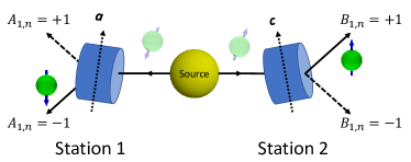
Figure 1: (color online) Conceptual representation of the Einstein-Podolsky-Rosen experiment [1] in the modified form proposed by Bohm [2]. A source produces pairs of particles. The particles of each pair carry opposite magnetic moments, implying that there is a correlation between the two magnetic moments of each pair leaving the source. The magnetic field gradients of the Stern-Gerlach magnets (cylinders) with their uniform magnetic field component along the directions of the unit vectors $\mathbf{a}$ and $\mathbf{c}$ divert each incoming particle into one of the two spatially separated directions labeled by $+1$ and $-1$. The pair $(\mathbf{a},\mathbf{c})$ represents the conditions, denoted by the subscript “$1$”, under which the discrete data $(A_{1,n},B_{1,n})$ is collected. The values of $A_{1,n}$ and $B_{1,n}$ correspond to the labels of the directions in which the particles have been diverted. The result of this experiment is the set of data pairs ${\cal D}_{1}=\{(A_{1,1},B_{1,1}),\ldots,(A_{1,N_{1}},B_{1,N_{1}})\}$ where $N_{1}$ denotes the number of pairs emitted by the source. The alternative conditions $(\mathbf{a},\mathbf{d})$, $(\mathbf{b},\mathbf{c})$, and $(\mathbf{b},\mathbf{d})$ are labeled by subscripts “$2$”, “$3$”, and “$4$”, respectively.

In general, each correlation $C_{s}$ may take values $-1$ or $+1$, independent of the values taken by other contributions, yielding the trivial bound $|C_{1}\mp C_{2}|+|C_{3}\pm C_{4}|\leq 4$. Without introducing a specific model for the process generating the data, we can derive a nontrivial bound that is sharper by exploiting the commutative property of addition.

Let $K_{\mathrm{max}}$ be the maximum number of quadruples $(x_{k},y_{k},z_{k},w_{k})$ that can be found by searching for permutations $P$, ${\widehat{P}}$, ${\widetilde{P}}$, and $P^{\prime}$ of $\{1,2,\ldots,N\}$ such that for $k=1,\ldots,K_{\mathrm{max}}$,

$$x_{k} =A_{1,P(k)}=A_{2,{\widehat{P}}(k)}\;, \;y_{k} =A_{3,{\widetilde{P}}(k)}=A_{4,P^{\prime}(k)}\;,$$

$$z_{k} =B_{1,P(k)}=B_{3,{\widetilde{P}}(k)}\;, \;w_{k} =B_{2,{\widehat{P}}(k)}=B_{4,P^{\prime}(k)}\;.$$ (3)

These quadruples are found by rearranging/reshuffling the data in ${\cal D}_{1}$, ${\cal D}_{2}$, ${\cal D}_{3}$, and ${\cal D}_{4}$ without affecting the value of the correlations $C_{1}$, $C_{2}$, $C_{3}$, and $C_{4}$.

Theorem: For any (real or computer or thought) EPRB experiment, the correlations Eq. (2) computed from the four data sets ${\cal D}_{1}$, ${\cal D}_{2}$, ${\cal D}_{3}$, and ${\cal D}_{4}$, must satisfy the model-free inequalities

$${\cal C}_{\pm}=\left|C_{1}\mp C_{2}\right|+\left|C_{3}\pm C_{4}\right|\leq 4-2{\Delta}\;,$$ (4)

where $0\leq{\Delta}=K_{\mathrm{max}}/N\leq 1$.

Proof: We rewrite the correlations in Eq. (2) as

$$C_{1} =\frac{1}{N}\sum_{n=1}^{N}A_{1,{P}(n)}B_{1,{P}(n)}, \;C_{2} =\frac{1}{N}\sum_{n=1}^{N}A_{2,{\widehat{P}}(n)}B_{2,{\widehat{P}}(n)}\;,$$

$$C_{3} =\frac{1}{N}\sum_{n=1}^{N}A_{3,{\widetilde{P}}(n)}B_{3,{\widetilde{P}}(n)}, \;C_{4} =\frac{1}{N}\sum_{n=1}^{N}A_{4,P^{\prime}(n)}B_{4,P^{\prime}(n)}\;.$$ (5)

Obviously, reordering the terms of the sums does not change the value of the sums themselves. As $|x_{k}|=|y_{k}|=|z_{k}|=|w_{k}|=1$, we (trivially) have $|x_{k}z_{k}-x_{k}w_{k}|+|y_{k}z_{k}+y_{k}w_{k}|=2$.

Splitting each of the sums in Eq. (5) into a sum over $k=1,\ldots,K_{\mathrm{max}}$ and the sum of the remaining terms, application of the triangle inequality yields

$${\cal C}_{\pm} \leq \frac{2K_{\mathrm{max}}}{N}$$ (6)

$$+\frac{1}{N}\sum_{n=K_{\mathrm{max}}+1}^{N}\left(\left|A_{1,{P}(n)}B_{1,{P}(n)}\right|+\left|A_{2,{\widehat{P}}(n)}B_{2,{\widehat{P}}(n)}\right|\right.$$

$$\hbox to56.9055pt{}\left.+\left|A_{3,{\widetilde{P}}(n)}B_{3,{\widetilde{P}}(n)}\right|+\left|A_{4,P^{\prime}(n)}B_{4,P^{\prime}(n)}\right|\right)$$

$$\leq \frac{2K_{\mathrm{max}}}{N}+\frac{4(N-K_{\mathrm{max}})}{N}=4-2{\Delta}\;.$$

QED.

In the same manner, one can prove a model-free version of the Clauser-Horne inequality [14, 15], applicable to the data of the EPRB experiments reported in Ref. 9, 10.

The choice represented by Eq. (3) is motivated by the EPRB experiment, see Fig. 1. In general, other choices to define quadruples are possible and may yield different values of the maximum fraction of quadruples.

We introduce the Bell-CHSH-like function

$${S}=\max_{p}\left|C_{p(1)}-C_{p(2)}+C_{p(3)}+C_{p(4)}\right|\;,$$ (7)

where the maximum is over all permutations $p$ of $\{1,2,3,4\}$. The maximum guarantees that we cover all possible expressions of the original Bell-CHSH function [13, 16, 12]. By application of the triangle inequality, it directly follows from Eq. (4) that, in the case of data collected by EPRB experiments,

$${S}\leq 4-2\Delta\;.$$ (8)

The symbol ${\Delta}$ in Eqs. (4) and (8) quantifies structure in terms of quadruples which can be created by relabeling the pairs of data in the sets ${\cal D}_{1}$, ${\cal D}_{2}$, ${\cal D}_{3}$, and ${\cal D}_{4}$. If ${\Delta}=0$, it is impossible to find a reshuffling that yields even one quadruple. If ${\Delta}=1$, the four sets can be reshuffled such that they can be viewed as being generated from $N$ quadruples. In the special case ${\Delta}=1$, we recover the model-free version of the Bell-CHSH inequality

$${S}\leq 2\;.$$ (9)

Traditionally, Eq. (9) is proven by assuming that the data can be modeled by a so-called “local realistic” (Bell) model [13, 16, 14, 15, 12]. However, this proof does not extend to the much more general case of the data generated by EPRB experiments, in contrast to the proof of Eq. (9) which holds for experimental data.

The proof of the model-free inequalities Eqs. (4) and (8) only requires the existence of a maximum number of quadruples, the actual value of this maximum being irrelevant for the proof. However, it is instructive to write a computer program that uses pseudo-random numbers to generate the data sets ${\cal D}_{1}$, ${\cal D}_{2}$, ${\cal D}_{3}$, and ${\cal D}_{4}$ and finds the number of quadruples. We have implemented the computer program in Mathematica^®.

Naively, finding the value of ${\Delta}$ seems to require ${\cal O}(N!^{4})$ operations. Fortunately, the problem of determining the fraction of quadruples ${\Delta}$ can be cast into an integer linear programming problem which is readily solved by considering the associated linear programming problem with real-valued unknowns. In practice, we solve the latter by standard optimization techniques [17]. For all cases that we have studied, the solution of the linear programming problem takes integer values only. Then the solution of the linear programming problem is also the solution of the integer programming problem.

The results of several numerical experiments using $N=1000000$ pairs per data set can be summarized as follows:

• If the $A$’s and $B$’s are generated in the form of quadruples, all items taking random values $\pm 1$, the program returns ${\Delta}=1$, $|C_{1}-C_{2}|+|C_{3}+C_{4}|=0.00063$, and $|C_{1}+C_{2}|+|C_{3}-C_{4}|=0.0028$ such that Eq. (4) is satisfied.

• If all $A$’s and $B$’s take independent random values $\pm 1$, the $C$’s are approximately zero. We have $|C_{1}\mp C_{2}|+|C_{3}\pm C_{4}|\approx 0\leq 4-2{\Delta}$ where in our particular numerical experiment ${\Delta}=0.998$.

• If the pairs $(A_{1,i},B_{1,i})$, $(A_{2,j},B_{2,j})$, $(A_{3,k}B_{3,k})$, and $(A_{4,l}B_{4,l})$ are generated randomly with frequencies $(1-c_{1}A_{1,i}B_{1,i})/4$, $(1-c_{2}A_{2,j}B_{2,j})/4$, $(1-c_{3}A_{3,k}B_{3,k})/4$, and $(1-c_{4}A_{4,l}B_{4,l})/4$, respectively, the simulation mimics the case of the correlation of two spin-1/2 objects in the singlet state if we choose $c_{1}=-c_{2}=c_{3}=c_{4}=1/\sqrt{2}$. In this particular case, quantum theory yields $\max\left(|C_{1}-C_{2}|+|C_{3}+C_{4}|,|C_{1}+C_{2}|+|C_{3}-C_{4}|\right)=2\sqrt{2}\approx 2.83$ [18].

  Generating four times one million independent pairs, we obtain ${\Delta}\approx 0.585$, ${S}=|C_{1}-C_{2}|+|C_{3}+C_{4}|\approx 2.83$ and $4-2{\Delta}\approx 2.83$, demonstrating that the value of the quantum-theoretical upper bound $2\sqrt{2}$ is reflected in the maximum fraction of quadruples that one can create by reshuffling the data.

• In the case of Bell’s model, slightly modified to comply with Malus’ law, we have $C_{1}=-\mathbf{a}\cdot\mathbf{c}/2$ and ${S}\leq\sqrt{2}$. Choosing $c_{1}=-c_{2}=c_{3}=c_{4}=1/(2\sqrt{2})$ and generating four times one million independent pairs, we obtain $S=|C_{1}-C_{2}|+|C_{3}+C_{4}|\approx 1.42$ and $4-2{\Delta}\approx 2.00$, as expected for Bell’s local realistic model.

Except for the first case, the numerical values of ${\Delta}$ quoted fluctuate a little if we repeat the $N=1000000$ simulations with different random numbers. In the third case, the simulations suggest that inequality Eq. (4) can be saturated.

Suppose that the (post-processed) data of an EPRB laboratory experiment yield ${S}>2$, that is the data violate inequality Eq. (9). From Eq. (8), it follows that ${\Delta}\leq 2-{S}/2<1$ if ${S}>2$. Therefore, if ${S}>2$ not all the data in ${\cal D}_{1}$, ${\cal D}_{2}$, ${\cal D}_{3}$, and ${\cal D}_{4}$ can be reshuffled such that they form quadruples only. Indeed, the data produced by these experiments have to comply with Eq. (8) which follows from Eq. (4) holding for data, and certainly do not have to comply with the original Bell-CHSH inequality obtained from Bell’s model.

In other words, all EPRB experiments which have been performed and may be performed in the future and which only focus on demonstrating a violation of Eq. (9) merely provide evidence that not all contributions to the correlations can be reshuffled to form quadruples (yielding ${\Delta}<1$). These violations do not provide any clue about the nature of the physical processes that produce the data.

More specifically, Eq. (4) holds for discrete data, irrespective of how the data sets ${\cal D}_{1}$, ${\cal D}_{2}$, ${\cal D}_{3}$, and ${\cal D}_{4}$ were obtained. Inequality (4) shows that correlations of discrete data violate the Bell-CHSH inequality Eq. (9) only if not all the pairs of data in Eq. (2) can be reshuffled to create quadruples. The proofs of Eq. (4) and Eq. (9) do not refer to notions such as “locality”, “realism”, “non-invasive measurements”, “action at a distance”, “free will”, “superdeterminism”, “(non)contextually”, “complementarity”, etc. Logically speaking, a violation of Eq. (9) by experimental data cannot be used to argue about the relevance of one or more of these notions to the process that generated the experimental data.

The existence of the divide between the realm of experimental EPRB data and mathematical models thereof is further supported by Fine’s theorem [19, 20]. Of particular relevance to the present discussion is the part of the theorem that establishes the Bell-CHSH inequalities (plus compatibility) as being the necessary and sufficient conditions for the existence of a joint distribution of the four observables involved in these inequalities. This four-variable joint distribution returns the pair distributions describing the four EPRB experiments required to test for a violation of these inequalities. Fine’s theorem holds in the realm of mathematical models only. Only in the unattainable limit of an infinite number of measurements (that is by leaving the realm of experimental data), and in the special case that the Bell-CHSH inequalities hold, it may be possible to prove the equivalence between the model-free inequality Eq. (9) and the Bell-CHSH inequality [13, 16, 14, 12].

A violation of the original (non model-free) Bell-CHSH inequality $S\leq 2$ may lead to a variety of conclusions about certain properties of the mathematical model for which this inequality has been derived. However, projecting these logically correct conclusions about the mathematical model, obtained within the context of that mathematical model, to the domain of EPRB laboratory experiments requires some care, as we now discuss.

The first step in this projection is to feed real-world, discrete data into the original Bell-CHSH inequality $S\leq 2$ derived, not for discrete data as we did by considering the case ${\Delta}=1$ in Eq. (8), but rather in the context of some mathematical model, and to conclude that this inequality is violated. Considering the discrete data for the correlations as given, it may indeed be tempting to plug these rational numbers into an expression obtained from some mathematical model. However, then it is no longer clear what a violation actually means in terms of the mathematical model because the latter (possibly by the help of pseudo-random number generators) may not be able to produce these experimental data at all. The second step is to conclude from this violation that the mathematical model cannot produce the numerical values of the correlations, implying that the mathematical model simply does not apply and has to be replaced by a more adequate one or that one or more premises underlying the mathematical model must be wrong. In the latter case, the final step is to project at least one of these wrong premises to properties of the world around us.

The key question is then to what extent the premises or properties of a mathematical model can be transferred to those of the world around us. Based on the rigorous analysis presented in this paper, the authors’ point of view is that in the case of laboratory EPRB experiments, they cannot.