Error analysis for a Crouzeix–Raviart approximation of the obstacle problem
Abstract
In the present paper, we study a Crouzeix–Raviart approximation of the obstacle problem, which imposes the obstacle constraint in the midpoints (i.e., barycenters) of the elements of a triangulation. We establish a priori error estimates imposing natural regularity assumptions, which are optimal, and the reliability and efficiency of a primal-dual type a posteriori error estimator for general obstacles and involving data oscillation terms stemming only from the right-hand side. Numerical experiments are carried out to support the theoretical findings.
Keywords: Obstacle problem; Crouzeix–Raviart element; a priori error analysis; a posteriori error analysis.
AMS MSC (2020): 35J20; 49J40; 49M29; 65N30; 65N15; 65N50.
1. Introduction
The obstacle problem is a prototypical example of a non-smooth convex minimization problem with an inequality constraint that leads to a variational inequality. It has countless applications, e.g., in the contexts of fluid filtration in porous media, constrained heating, elasto-plasticity, optimal control, and financial mathematics, cf. [14, 29]. It is deeply related to models in free boundary value problems, the study of minimal surfaces, and the capactity of a set in potential theory, cf. [14]. The problem is to find the equilibrium position of an elastic membrane whose boundary is held fixed and which is constrained to lie above a given obstacle.
More precisely, given an external force and an obstacle with on , where denotes the Dirichlet part of the topological boundary , the obstacle problem seeks for a minimizer of the energy functional , for every defined by
| (1.1) |
where
and is defined by if and else.
Related contributions
The numerical approximation of (1.1) has already been the subject of numerous contributions: Early contributions examing the a priori and a posteriori error analysis of approximations of (1.1) using the conforming Lagrange finite element can be found in [26, 1, 32, 37, 38, 13, 43, 17, 42, 10, 11, 9, 48, 27], imposing the obstacle constraint in the nodes of a triangulation, and in [34, 28], enforcing the obstacle constraint in the limit via a penalization approach. We refer to [17] for a short review. Contributions addressing the a priori and a posteriori error analysis of an approximation of (1.1) deploying Discontinuous Galerkin (DG) type methods can be found in [30, 18, 5], equally imposing the obstacle constraint in the nodes of a triangulation. The first contribution addressing the a priori error analysis of an approximation of (1.1) in two dimensions deploying the Crouzeix–Raviart element can be found in [47] and imposes the obstacle constraint in the midpoints (i.e., barycenters) of elements of a triangulation. In [6], for homogeneous Dirichlet boundary data and zero obstacle, this result was extended to arbitrary dimensions. In [15], an a priori and a posterior error analysis of an approximation of (1.1) deploying the Crouzeix–Raviart element which imposes the obstacle constraint in the integral mean values of element sides of a triangulation was carried out.
New contributions
Inspired by [47] as well as recent contributions [5, 6, 7], different from the contribution [15], we treat an approximation of the obstacle problem (1.1) deploying the Crouzeix–Raviart element that imposes the obstacle constraint in the midpoints (i.e., barycenters) of elements of a triangulation. More precisely, given a family of regular triangulations , , setting and for approximating , our discrete obstacle problem seeks for a minimizer of the functional , for every defined by
| (1.2) |
where
and is defined by if and else. Here, denotes the space of element-wise constant functions, the Crouzeix–Raviart finite element space, i.e., the space of element-wise affine functions that are continuous in the midpoints (i.e., barycenters) of inner element sides and that vanish in the midpoints of element sides that belong to , the element-wise gradient and the (local) -projection operator onto element-wise constant functions. Imposing the obstacle constraint in the midpoints of elements follows a systematic approximation procedure for general convex minimization problems deploying the Crouzeix–Raviart element introduced in [6, 7] and has the advantage that the resulting discrete convex minimization problem generates discrete convex duality relations that are analogous to those in the continuous setting –up to non-conforming modifications– and that enable a systematic a priori error analysis and a posteriori error analysis:
-
In [6], a systematic procedure for the derivation of a priori error estimates for convex minimi-zation problems deploying the Crouzeix–Raviart element based on (discrete) convex duality relations was proposed. Following this systematic procedure, with comparably little effort, we derive a priori error estimates, which are optimal for natural regularity assumptions and also apply in arbitrary dimensions. More precisely, our a priori error estimates exploit that the discrete primal-dual gap controls the convexity measure of (1.2) and the concavity measure of its dual functional, i.e., that for every and , it holds
(1.3) where denotes the Raviart–Thomas finite element space, i.e., the space of element-wise affine vector fields that have continuous constant normal components on element sides that vanish on , the unique discrete dual solution, i.e., the maximizer of the discrete dual energy functional , and the unique discrete Lagrange multiplier satisfying a.e. in and for all
If , where denotes the Crouzeix–Raviart quasi-interpolation operator, then . Thus, under natural regularity assumptions, i.e., , the choices and , where denotes the dual solution, i.e., the maximizer of the dual energy functional , and the Raviart–Thomas quasi-interpolation operator, are admissible in (1.3) and lead to quasi-optimal a priori error estimates.
-
In [7], a systematic procedure for the derivation of reliable, quasi-constant-free a posteriori error estimates for convex minimization problems deploying the Crouzeix–Raviart element ba-sed on (discrete) convex duality relations was proposed. Following this systematic procedure, we derive a posteriori error estimates, which, by definition, are reliable and constant-free. Apart from that, we establish the efficiency of these a posteriori error estimates for general obstacles . More precisely, our a posteriori error estimates exploit that the primal-dual gap controls the convexity measure of (1.1) and the concavity measure of its dual functional, i.e., that for every and , it holds
(1.4) where is the unique Lagrange multiplier satisfying in and for all
For the a posteriori error estimate (1.4) being practicable it is necessary to have a sufficiently accurate and computationally cheap procedure to obtain an approximation of the dual solution at hand. In the case , the discrete dual solution is admissible in (1.4) and leads to a constant-free reliable and efficient a posteriori error estimator , which has similarities to the residual type a posteriori estimator derived in [42] but is simper and avoids jump terms of the obstacle that arise in the efficiency analysis in [42]. In particular, note that the discrete dual solution can cheaply be computed via the generalized Marini formula
(1.5) A typical choice of is obtained via nodal averaging and truncating to enforce the continuous obstacle constraint. Moreover, any conforming approximation can be used such as a continuous Lagrange approximation , so that our analysis also implies the full reliability and efficiency error analysis for continuous Lagrange approximations, even for general obstacles and oscillation terms only stemming from the right-hand side since lumping is not needed in our analysis.
As a whole, our approach brings together and extends ideas and concepts from [13, 43, 42, 10, 11, 15], and leads to a full error analysis.
Outline
This article is organized as follows: In Section 2, we introduce the notation, the relevant function spaces and finite element spaces. In Section 3, we give a brief review of the continuous and the discrete obstacle problem. In Section 4, we prove a priori error estimates for the Crouzeix–Raviart approximation (1.2) of (1.1), which are optimal for natural regularity assumptions. In Section 5, we introduce a primal-dual a posteriori error estimator and establish its reliability and efficiency. In Section 6, numerical experiments are carried out to confirm the theoretical findings. In the Appendix A, we derive local efficiency estimates for the Crouzeix–Raviart approximation (1.2) of (1.1).
2. Preliminaries
Throughout the article, let , , be a bounded polyhedral Lipschitz domain whose boundary is disjointly divided into a closed Dirichlet part , for which we assume that 111For a (Lebesgue) measurable set , , we denote by its -dimensional Lebesgue measure. For a -dimensional submanifold , , we denote by its -dimensional Hausdorff measure., and a Neumann part . For (Lebesgue) measurable functions and a (Lebesgue) measurable set , we employ the product
whenever the right-hand side is well-defined. Analogously, for (Lebesgue) measurable vector fields and a (Lebesgue) measurable set , we write .
Standard function spaces
For , we let
in the case , and in the case . Here, and denote the trace and normal trace operator, respectively. More precisely, on for all , where denotes the outer unit normal vector field to . We always omit and . For a compact notation, we abbreviate , , , , , and , .
Triangulations and standard finite element spaces
Throughout the article, let , , be a family of uniformly shape regular and conforming, triangulations of , , cf. [25]. Here, the parameter denotes the average mesh-size, i.e., , where for all . We assume there exists , independent of , such that , where for all . The smallest such constant is called the chunkiness of . For every , let denote the element patch of . Then, we assume that is connected for all , so that , where depends only on the chunkiness , and for all . Eventually, we define the maximum mesh-size by .
We define interior and boundary sides of in the following way: an interior side is the closure of the non-empty relative interior of , where are two adjacent elements. For an interior side , where , the side patch is defined by . A boundary side is the closure of the non-empty relative interior of , where denotes a boundary element of . For a boundary side , the side patch is defined by . Eventually, by , we denote the set of interior sides, and by , we denote the set of all sides.
For (Lebesgue) measurable functions and , we employ the product
whenever all integrals are well-defined. Analogously, for (Lebesgue) measurable vector fields and , we write , where .
For and , let denote the set of polynomials of maximal degree on . Then, for and , the sets of continuous and element-wise polynomial functions or vector fields, respectively, are defined by
The element-wise constant mesh-size function is defined by for all . The side-wise constant mesh-size function is defined by for all , where for all . If contains the vertices of , for every and , we denote by and , the barycenters of and , respectively. Moreover, the (local) -projection operator onto element-wise constant functions or vector fields, respectively, is denoted by
There exists a constant , depending only on the chunkiness , such that for every , , and , cf. [25, Theorem 18.16], it holds
-
(L0.1)
,
-
(L0.2)
if .
Crouzeix–Raviart element
The Crouzeix–Raviart finite element space, cf. [19], is defined as space of element-wise affine functions that are continuous in the barycenters of inner element sides, i.e.,222Here, for every inner side , the jump is defined by on , where satisfy , and for every boundary side , the jump is defined by on , where satisfies .
The Crouzeix–Raviart finite element space with homogeneous Dirichlet boundary condition on is defined as the space of Crouzeix–Raviart finite element functions that vanish in the barycenters of boundary element sides that belong to , i.e.,
The functions , , that satisfy the Kronecker property for all , form a basis of . Then, the functions , , form a basis of . There exists a constant , depending only on the chunkiness , such that for every , it holds the discrete Poincaré inequality
| (2.1) |
where , , defined by for all and , is the element-wise gradient. The quasi-interpolation operator , for every defined by
| (2.2) |
preserves averages of gradients, i.e., in for every . There exists a constant , depending only on the chunkiness , such that for every and , cf. [22, Remark 4.4 & Theorem 4.6], it holds
-
(CR.1)
,
-
(CR.2)
,
-
(CR.3)
if .
Raviart–Thomas element
The Raviart–Thomas finite element space (of lowest order), cf. [41], is defined as the space of element-wise affine vector fields that have continuous constant normal components on inner elements sides, i.e.,333For every inner side , the normal jump is defined by on , where satisfy , and for every , denotes the outward unit normal vector field to , and for every boundary side , the normal jump is defined by on , where satisfies .
The Raviart–Thomas finite element space with homogeneous slip boundary condition on is defined as the space of Raviart–Thomas vector fields whose normal components vanish on , i.e.,
The vector fields , , that satisfy the Kronecker property on for all , where for all is the unit normal vector on pointing from to if , form a basis of . Then, the vector fields , form a basis of . The quasi-interpolation operator , for every defined by
| (2.3) |
preserves averages of divergences, i.e., in for every . There exists a constant , depending only on the chunkiness , such that for every and , cf. [25, Theorem 16.4], it holds
-
(RT.1)
,
-
(RT.2)
,
-
(RT.3)
.
Discrete integration-by-parts formula
For every and , it holds the discrete integration-by-parts formula
| (2.4) |
which follows from the fact that, by definition, for every , it holds on for all and on for all , and for every , it holds for all . As a result, for every and , (2.4) reads
| (2.5) |
In [16, 5, 6, 7], the discrete integration-by-parts formula (2.5) formed a cornerstone in the derivation of a discrete convex duality theory and, as such, also plays a central role in the hereinafter analysis. For instance, cf. [6, Lemma 2.1], for every and , (2.5) enables to exchange quasi-interpolation operators via
| (2.6) |
In addition, cf. [8, Section 2.4], there holds the orthogonal decomposition
| (2.7) |
3. Obstacle problem
In this section, we discuss the continuous and the discrete obstacle problem.
Continuous obstacle problem
Primal problem. Given a force and an obstacle with on , the (continuous) obstacle problem is defined via the minimization of , for every defined by
| (3.1) |
where
and is given via if and else. In what follows, we refer to the minimization of the functional (3.1) as the primal problem. Since the functional (3.1) is proper, strictly convex, weakly coercive, and lower semi-continuous, cf. [3, Theorem 5.1], the direct method in the calculus of variations, cf. [20], yields the existence of a unique minimizer , called the primal solution. In what follows, we reserve the notation for the primal solution. Since the functional (3.1) is not Fréchet differentiable, the optimality conditions associated with the primal problem are not given via a variational equality. Instead, they are given via a variational inequality. In fact, cf. [3, Theorem 5.2], is minimal for (3.1) if and only if for every
| (3.2) |
Dual problem. Appealing to [24, Section 2.4, p. 84 ff.], the dual problem to the obstacle problem is defined via the maximization of , for every defined by
| (3.3) |
where is defined by if for all and else, is defined by for all and , and is defined by for all . For every , there holds the representation
| (3.4) |
where is defined by if with a.e. in and else. Moreover, in [24, Section 2.4, p. 84 ff.], it is shown that there exists a unique maximizer of (3.3), called the dual solution, and a strong duality relation, i.e.,
| (3.5) |
applies. In addition, there hold the convex optimality relations
| (3.6) | |||
| (3.7) |
Augmented problem. Due to [3, Theorem 5.2], there exists a Lagrange multiplier with in , i.e., for all with for a.e. , such that for every , it holds the augmented problem
| (3.8) |
i.e., in . Then, cf. [3, Theorem 5.2], there holds the complementary condition
| (3.9) |
If there exists such that for all , cf. [36], then (3.9) reads
| (3.10) |
Discrete obstacle problem
Discrete primal problem. Given a force and an obstacle such that on , with and approximating , the discrete obstacle problem is defined via the minimization of , for every defined by
| (3.11) |
where
and is given via if and else. In what follows, we refer to the minimization of the functional (3.11) as the discrete primal problem. Since the functional (3.11) is proper, strictly convex, weakly coercive, and lower semi-continuous, the direct method in the calculus of variations, cf. [20], yields the existence of a unique minimizer , called the discrete primal solution. In what follows, we reserve the notation for the discrete primal solution. In addition, is the unique minimizer of (3.11) if and only if for every , it holds
| (3.12) |
Discrete dual problem. Appealing to [6, Subsection 4.1], the discrete dual problem to the discrete obstacle problem is defined via the maximization of , for every defined by
| (3.13) |
Discrete augmented problem. The discrete augmented problem, similar to the augmented problem (3.8), seeks for a discrete Lagrange multiplier such that a.e. in and for every , it holds
| (3.14) |
The following proposition establishes the well-posedness of the discrete augmented problem (3.14).
Proposition 3.1.
The following statements apply:
-
(i)
The discrete augmented problem is well-posed, i.e., there exists a unique discrete Lagrange multiplier that satisfies (3.14).
-
(ii)
The discrete Lagrange multiplier satisfies a.e. in and the discrete complementarity condition
(3.15)
Remark 3.2.
Proof (of Proposition 3.1)..
ad (i). We relax the obstacle constraint via a penalization scheme, i.e., for every , we consider the minimization of , for every defined by
Since for any , is continuous, strictly convex, and weakly coercive, the di-rect method in the calculus of variation yields the existence of a unique minimizer , which, for every , abbreviating , satisfies
| (3.16) |
Due to the minimality of , we find that and, as a consequence,
using that a.e. in , that
| (3.17) |
Using the -Young inequality , valid for all and , (L0.1), and the discrete Poincaré inequality (2.1), for every , we find that
| (3.18) |
Using (3.18) for in (3.17), for every , we arrive at
| (3.19) |
Using the discrete Poincaré inequality (2.1) in (3.19), we find that is bounded. Hence, owing to the finite dimensionality of , we deduce the existence of such that, for a not re-labeled subsequence, it holds
| (3.20) |
Let for every and be defined by
| (3.21) |
Then, from (3.16), also using (L0.1), for every , it follows that
| (3.22) |
Using (3.19) in (3.22), we find that is bounded. Thus, due to the finite dimensionality of and the closedness of the range , there exists with
| (3.23) |
Next, using (3.19) once more and that, by definition, , we deduce that
Because, on the other hand, due to (3.20), in , we conclude that a.e. in . In other words, we have that
| (3.24) |
As a consequence of (3.24), for every and , resorting to (3.20) and the minimality of for , we find that
Hence, due to the uniqueness of as a minimizer of , we infer that in . By passing for in (3.16), for every , using (3.20), (3.23), and the definition of , cf. (3.21), we conclude that
| (3.25) |
Owing to , there exist unique and such that in . By the aid of the latter decomposition, for every , we conclude from (3.25) that
Next, let be such that for every , it holds
Then, and, thus, in .
ad (ii). Let be such that . For each , there exists such that . Next, let be such that a.e. in . Then, for in (3.14), in particular, using (3.12) for , we deduce that
| (3.26) |
As was arbitrary and , we conclude from (3.26) that a.e. in . Eventually, for such that a.e. in , there exists some such that a.e. in . For this in (3.26), also using that a.e. in , we arrive at
so that a.e. in . In other words, it holds (3.15). ∎
Given a discrete Lagrange multiplier satisfying (3.14), we define the discrete flux
| (3.27) |
which, by definition, satisfies
| (3.28) |
The following proposition proves that the discrete flux is admissible in the discrete dual problem and even a discrete dual solution.
Proposition 3.3.
The following statements apply:
-
(i)
The discrete flux satisfies and
(3.29) In particular, it holds a.e. in , i.e., .
-
(ii)
The discrete flux is a maximizer of (3.13) and discrete strong duality, i.e., , applies. In addition, there holds the discrete complementary condition
(3.30)
Proof.
ad (i). Since, due to , is surjective, there exists some such that in . Then, using the discrete integration-by-parts formula (2.5) and (3.14), for every , we find that
| (3.31) |
Using (3.28) in (3.31), for every , we arrive at
| (3.32) |
On the other hand, we have that a.e. in for all , so that . Hence, by (3.32) and the orthogonal decomposition (2.7), we conclude that and, thus, , since already .
4. A priori error analysis
In this section, we establish a priori error estimates for the discrete primal problem.
Theorem 4.1.
If , i.e., and , and , then there exists a constant , depending only on the chunkiness , such that
Proof.
Using that, owing to the discrete augmented problem (3.14), for all , and the strong concavity of (3.13), for every and , it holds
that , as and for all and with , that with a.e. in , the discrete strong duality relation , cf. Proposition 3.3 (ii), in , (L0.1), and the strong duality relation , cf. (3.5), we find that
| (4.1) |
Next, using in (4.1) the exchange of quasi-interpolation operators (2.6) and , cf. (3.6), i.e.,
in , and in , abbreviating , we get
| (4.2) |
As a consequence, it remains to estimate the terms , and :
ad . Using (CR.3), we obtain
| (4.3) |
ad . Using that in , in , in , and (CR.3), we obtain
| (4.4) |
Corollary 4.2.
If , then there exists a constant , depending only on the chunkiness , such that
5. A posteriori error analysis
In this section, we examine the primal-dual a posteriori error estimator , for every defined by
| (5.1) |
for reliability and efficiency.
Remark 5.1.
-
(i)
The estimator appeared in a similar form in [15] in a Crouzeix–Raviart approximation of the obstacle problems, imposing the obstacle constraint at the barycenters of element sides. However, imposing the obstacle constraint at the barycenters of elements leads to a simplified form compared to the estimator in [15].
-
(ii)
The estimator provides control over the flux relation (3.6).
- (iii)
-
(iv)
The estimator measures the irregularity of the dual solution, i.e., .
Reliability
In this subsection, we identify error quantities that are controlled by the a posteriori error estimator , cf. (5.1). In doing so, we combine two different but related approaches: first, we resort to first-order relations based on (discrete) convex duality, leading to constant-free estimates; second, we resort to second-order relations based on the (discrete) augmented problems, leading to estimates for further error quantities that are not covered be the first approach.
Reliability based on (discrete) convex duality
In this subsection, we follow the procedure for the derivation of, by definition, reliable and con-stant-free a posteriori error estimates based on (discrete) convex duality outlined in the introduction.
Lemma 5.2.
For every , we have that
Proof.
Using that, owing to the augmented problem (3.8), for all , and the strong concavity of (3.3), for every and , it holds
| (5.2) | ||||
| (5.3) |
the strong duality relation , cf. (3.5), that with a.e. in , cf. (3.29), integration-by-parts, and in , cf. (3.28), we get
Due to in , cf. (3.27), we conclude the assertion. ∎
Remark 5.3.
Remark 5.4.
The reliability estimate in Lemma 5.2 is entirely constant-free.
Remark 5.5 (Improved reliability).
If we have that in Lemma 5.2, then, given in , we arrive at the improved reliability estimate
Corollary 5.6.
If , then the following statements apply:
-
(i)
For every , it holds
-
(ii)
For every , it holds
The a posteriori error estimator , cf. (5.1), furthermore, controls the error between the continuous Lagrange multiplier , defined by (3.8), and the discrete Lagrange multiplier , defined by (3.14), measured in the Sobolev dual norm. To this end, we introduce the -representation of , for every defined by
Lemma 5.7.
The following statements apply:
-
(i)
If we set , cf. Theorem A.1, then
(5.4) -
(ii)
If , then for every , it holds
(5.5)
Reliability based on variational equations
Following an approach which resorts to the (discrete) augmented problems, i.e., (3.8) and (3.14), it is possible to establish the following reliability result, which identifies additional quantities that are controlled by the a posteriori error estimator , cf. (5.1).
Lemma 5.9.
For every and , we have that
From Lemma 5.9 we can immediately deduce the following reliability results.
Corollary 5.10.
The following statements apply:
-
(i)
For every , it holds
-
(ii)
For every , it holds
Proof.
Having Corollary 5.10 (ii) at hand, by analogy with Lemma 5.7 (ii), we arrive at the following reliability result for the error between the continuous and the discrete Lagrange multiplier measured in the dual norm.
Corollary 5.11.
For every , we have that
Proof.
Proof (of Lemma 5.9)..
Resorting to (3.8), for every , since in , we find that
| (5.9) |
Resorting to (3.14), for every , we find that
| (5.10) |
i.e., owing to in and , for every
| (5.11) |
If we subtract (5.11) from (5.9), we arrive at
| (5.12) |
The binomial theorem shows that
| (5.13) |
Resorting to (CR.2), (L0.2) and the -Young inequality , valid for all and , for every , we find that
| (5.14) | ||||
| (5.15) |
Therefore, combining (5.12)–(5.14), we conclude the claimed inequality. ∎
Given the findings of Lemma 5.2, Lemma 5.9, and Lemma 5.7, we introduce the error measure , for every defined by
| (5.16) |
Theorem 5.12 (Reliability).
There exist constants , depending only on the chunkiness , such that for every , we have that
Remark 5.13 (Comments on the reliability constant ).
Efficiency
In this subsection, we show the efficiency of the a posteriori error estimator , cf. (5.1), with respect to the error measure , cf. (5.16).
Theorem 5.14 (Efficiency).
There exist constants , depending on the chunkiness , such that for every , we have that
Proof.
Remark 5.15.
Since the discrete primal solution is neither an admissible approx-imation of the primal solution in Theorem 5.12 nor in Theorem 5.14, since, in general,
it is necessary to post-process . In the numerical experiments, cf. Section 6, we employ the post-processed function , where is a node-aver-aging quasi-interpolation operator, cf. Subsection A.1, which, by the Sobolev chain rule, satisfies
i.e., . Note that in due to on and in . In addition, using the best-approximation property of , cf. Proposition A.4, we have that
and, thus,
In other words, the error between and (and , respectively) is controlled by the error between and plus a contribution capturing the violation of the continuous obstacle constraint by .
Remark 5.16.
Appealing to Theorem A.1 and Lemma A.3 (A.7), there exists a constant , depending only on the chunkiness , such that for every , we have that
Thus, it is possible to establish efficiency estimates for parts of the primal-dual a posteriori error estimator, which also apply for non-conforming functions, cf. Appendix A.
6. Numerical experiments
In this section, we review the theoretical findings of Section 4 and Section 5 via numerical experiments. All experiments were carried out using the finite element software package FEniCS (version 2019.1.0), cf. [39]. All graphics are created using the Matplotlib (version 3.5.1) library, cf. [33].
Implementation details
We approximate the discrete primal solution and the associated discrete Lagrange multiplier jointly satisfying the discrete augmented problem (3.14) via the primal-dual active set strategy interpreted as a super-linear converging semi-smooth Newton method, cf. [3, Subsection 5.3.1] or [31]. For sake of completeness, we will briefly outline important implementation details related with this strategy.
We fix an ordering of the element sides and an ordering of the elements , where and , such that444In practice, the element for which is found via searching and erasing a zero column (if existent) in the matrix leading to .
where because of , cf. [8, Corollary 3.2]. Then, if we define the matrices
| and, assuming for the entire section that , the vectors | ||||
the same argumentation as in [3, Lemma 5.3] shows that the discrete augmented problem (3.14) is equivalent to finding vectors such that
| (6.1) |
where for given , the mapping for every is defined by
More precisely, the discrete primal solution and the associated discrete Lagrange multiplier jointly satisfying the discrete augmented problem (3.14) as well as , respectively, are related by555Here, for every , , we denote by , the -th unit vector.
Next, define the mapping for every by
Then, the non-linear system (6.1) is equivalent to finding such that
By analogy with [4, Theorem 5.11], one finds that the mapping is Newton-differentiable at every and, with the (active) set
we have that
where for every are defined by if and else.
For a given iterate , one step of the semi-smooth Newton method, cf. [3, Subsection 5.3.1] or [31], determines a direction such that
| (6.2) |
Setting and , the linear system (6.2) can equivalently be re-written as
| (6.3) |
The semi-smooth Newton method can, thus, equivalently be formulated in the following form, which is a version of a primal-dual active set strategy.
Algorithm 6.1 (Primal-dual active set strategy).
Choose parameters and . Moreover, let and set . Then, for every :
-
(i)
Define the most recent active set
-
(ii)
Compute the iterate such that
-
(iii)
Stop if ; otherwise, increase and continue with step (i).
Remark 6.2 (Important implementation details).
-
(i)
Algorithm 6.1 converges super-linearly if is sufficiently close to the solution , cf. [31, Theorem 3.1]. Since the Newton-differentiability only holds in finite-dimensional situations and deteriorates as the dimension increases, the condition on the initial guess becomes more critical for increasing dimensions.
- (ii)
-
(iii)
Since only a finite number of active sets are possible, the algorithm terminates within a finite number of iterations at the exact solution . For this reason, in practice, the stopping criterion in step (iii) is reached with for some , in which case, one has that , provided is sufficiently small.
- (iv)
-
(v)
Global convergence of the algorithm and monotonicity, i.e., for can be proved if is an -Matrix, cf. [31, Theorem 3.2].
-
(vi)
Classical active set strategies define , which corresponds to the formal limit .
Numerical experiments concerning the a priori error analysis
In this subsection, we review the theoretical findings of Section 4.
For our numerical experiments, we choose , , , , so that the exact solution , for every defined by
satisfies . Therefore, Theorem 4.1 let us expect a convergence rate of about .
An initial triangulation , , is constructed by subdividing a rectangular Cartesian grid into regular triangles with different orientations. Refined triangulations , , where for all , are obtained by applying the red-refinement rule, cf. [45].
For the resulting series of triangulations , , we apply the primal-dual active set strategy (cf. Algorithm 6.1) to compute the discrete primal solution , , the discrete Lagrange multiplier , and, subsequently, resorting to (3.27), the discrete dual solution , . Afterwards, we compute the error quantities
| (6.4) |
For the determination of the convergence rates, the experimental order of convergence (EOC)
where for every , we denote by , either , , , , , , , or , respectively, is recorded.
For a series of triangulations , , obtained by uniform mesh refinement as described above, the EOC is computed and presented in Table 1 and Table 2. In each case, except for , we record a convergence ratio of about , , confirming the optimality of the a priori error estimates established in Theorem 4.1 and Corollary 4.2. For , we record a convergence ratio of about , .
| 1.359 | — | 0.732 | — | 1.094 | — | 0.656 | — | |
| 0.787 | 0.788 | 0.664 | 0.141 | 0.533 | 1.038 | 0.453 | 0.535 | |
| 0.380 | 1.048 | 0.324 | 1.034 | 0.260 | 1.033 | 0.212 | 1.097 | |
| 0.197 | 0.948 | 0.166 | 0.968 | 0.131 | 0.993 | 0.116 | 0.872 | |
| 0.099 | 0.996 | 0.082 | 1.008 | 0.067 | 0.974 | 0.059 | 0.967 | |
| 0.050 | 0.989 | 0.042 | 0.986 | 0.033 | 1.010 | 0.030 | 0.968 | |
| 0.025 | 0.998 | 0.021 | 1.001 | 0.017 | 0.980 | 0.015 | 0.993 | |
| expected | — | 1.00 | — | 1.00 | — | 1.00 | — | 1.00 |
| 0.262 | — | 0.490 | — | 1.849 | — | 1.223 | — | |
| 0.144 | 0.866 | 0.199 | 1.300 | 0.986 | 0.907 | 0.863 | 0.502 | |
| 0.044 | 1.706 | 0.072 | 1.461 | 0.453 | 1.123 | 0.397 | 1.122 | |
| 0.020 | 1.133 | 0.029 | 1.308 | 0.226 | 0.999 | 0.195 | 1.024 | |
| 0.006 | 1.732 | 0.009 | 1.636 | 0.108 | 1.064 | 0.092 | 1.086 | |
| 0.002 | 1.363 | 0.003 | 1.447 | 0.053 | 1.024 | 0.045 | 1.027 | |
| 0.001 | 1.618 | 0.001 | 1.535 | 0.026 | 1.027 | 0.022 | 1.036 | |
| expected | — | 1.00 | — | 1.00 | — | 1.00 | — | 1.00 |
Numerical experiments concerning a posteriori error analysis
In this subsection, we review the theoretical findings of Section 5. More precisely, we apply the -approximation (3.11) of the obstacle problem (3.1) in an adaptive mesh refinement algorithm based on local refinement indicators associated with the a posteriori error estimator , cf. (5.1). More precisely, for every and , we define
Before we present numerical experiments, we briefly outline the details of the implementations. In general, we follow the adaptive algorithm, cf. [21]:
Algorithm 6.3 (AFEM).
Let , and a conforming initial triangulation of . Then, for every :
- (’Solve’)
-
Compute the discrete primal solution and the discrete Lagrange multiplier jointly solving the discrete augmented problem (3.14). Post-process to obtain a conforming approximation of the primal solution and a discrete dual solution .
- (’Estimate’)
-
Compute the local refinement indicators . If , then STOP; otherwise, continue with step (’Mark’).
- (’Mark’)
-
Choose a minimal (in terms of cardinality) subset such that
- (’Refine’)
-
Perform a conforming refinement of to obtain such that each is refined in . Increase and continue with step (’Solve’).
Remark 6.4.
- (i)
- (ii)
- (iii)
- (iv)
-
We always employ the parameter in (’Mark’).
- (v)
- (vi)
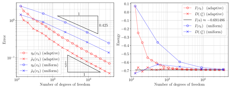
Example with corner singularity
We examine an example from [9]. In this example, we let , , , , in polar coordinates, for every defined by
where for every , abbreviating , are defined by
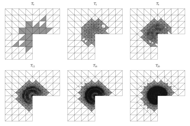
and . Then, the primal solution , in polar coordinates, for every defined by , has a singularity at the origin and, therefore, satisfies , so that we cannot expect uniform mesh refinement to yield the quasi-optimal linear convergence rate.
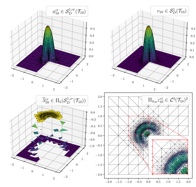
The coarsest triangulation of Figure 2 (and starting triagulation of Algorithm 6.3) consists of halved squares. More precisely, Figure 2 displays the triangulations , , generated by the adaptive Algorithm 6.3. The approximate contact zones , , are plotted in white Figure 2 while its complement is shaded666we chose this color as in most of the examples the complement of the contact zone is refined and appears darker.. Algorithm 6.3 refines in the complement of the contact zone . A refinement towards the origin, where the solution has a singularity in the gradient, and in , where the solution has large gradients, is reported. This behavior can also be seen in Figure 3, where the discrete primal solution , the node-averaged discrete primal solution , the discrete Lagrange multiplier , and the discrete dual solution are plotted on the triangulation , which has degrees of freedom. Figure 1 demonstrates that the adaptive Algorithm 6.3 improves the experimental convergence rate of about for uniform mesh-refinement to the optimal value . For uniform mesh-refinement, we expect an asymptotic convergence rate due to the corner singularity. Since not all quantities in the error measure are computable, in Figure 1, we employ the reduced error measure
where we exploit for the computation of the first two terms the identity (5.2).
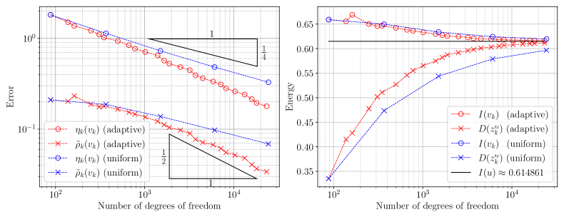
Example with unknown exact solution
We examine an example from [9]. In this example, we let , , , , and . The primal solution is not known and cannot be expected to satisfy inasmuch as , so that uniform mesh refine-ment is expected to yield a reduced error decay rate compared to the optimal linear error decay rate.
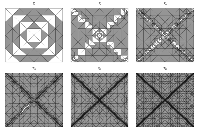
The coarsest triangulation in Figure 5 (and starting triangulation in Algorithm 6.3) consists of 64 elements. More precisely, Figure 5 displays the triangulations , , generated by the adaptive Algorithm 6.3. The approximate contact zones , , where for every , are plotted in white in Figure 5 while their complements are shaded. Note that for every , we have that and .
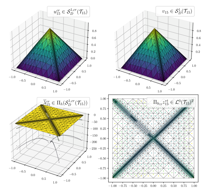
This example is different from the previous examples; in the sense that the solution and the obstacle are non-smooth along the lines . Algorithm 6.3 refines the mesh towards these lines as can be seen in Figure 5. In addition, the approximate contact zones , , reduces to . This behavior can also be observed in Figure 3, where the discrete primal solution , the node-averaged discrete primal solution , the discrete Lagrange multiplier , and the discrete dual solution are plotted on the triangulation , which has degrees of freedom. Algorithm 6.3 improves the experimental convergence rate of about for uniform mesh-refinement to the quasi-optimal value . Since not all quantities in the error measure are computable, in Figure 4, we employ the reduced error measure
where we exploit for the computation of the identity (5.2) and approximate the value via Aitken’s -process, cf. [2]. More precisely, we always employ the approximation , where the sequence , for every with , is defined by
However, it remains unclear whether this is a sufficiently accurate approximation of the exact errors , .
Appendix A Appendix
In this appendix, we derive local efficiency estimates for the Crouzeix–Raviart approximation (3.11) of (3.1), which, in turn, imply the following non-conforming efficiency result.
Theorem A.1.
There exists a constant , depending on the chunkiness , such that
where for every , we define , where for every , and .
The proof of Theorem A.1 involves two tools.
Node-averaging quasi-interpolation operator
The first tool is the node-averaging quasi-interpolation operator , that, denoting for every , by , the set of elements sharing , for every , is defined by
where we denote by , the nodal basis of . If , then, there exists a constant , depending on and the chunkiness , such that for every , , and , cf. [7, Appx. A.2], we have that
-
(AV.1)
,
-
(AV.2)
.
Local efficiency estimates
The second tool consists in local efficiency estimates that are based on standard bubble function techniques, cf. [44].
Lemma A.2.
There exists a constant , depending only the chunkiness , such that for every , , and , respectively, it holds
| (A.1) | ||||
| (A.2) |
where for every open set .
Proof.
ad (A.1). Let be fixed, but arbitrary. Then, there exists a bubble function such that in , in , and , where the constant depends only on the chunkiness . Using (3.8) and integration-by-parts, taking into account that and in doing so, for every , we find that
| (A.3) |
For the particular choice in (A.3) and applying the -Young inequality , valid for all and , also using that in and in , we observe that
| (A.4) | ||||
For the particular choice in (A.4), we conclude that (A.1) applies.
ad (A.2). Let be fixed, but arbitrary. Then, there exists a bubble function such that in , in , and , where the constant depends only on the chunkiness . Using (3.8) and integration-by-parts, taking into account that and in doing so, for every , we find that
| (A.5) |
Let be with . Then, for the particular choice in (A.5), for all , where depends only on the chunkiness , and applying the -Young inequality valid for all and , also using that in and in , we observe that
| (A.6) |
Using (A.6) and (A.1) in (A.5), for sufficiently small, conclude that (A.2) applies. ∎
From Lemma A.2 we can derive the following global efficiency result.
Lemma A.3.
There exists a constant , depending only the chunkiness , such that for every , it holds
| (A.7) | ||||
| (A.8) |
Proof of Theorem A.1
Finally, we have everything we need to prove the Theorem A.1.
Proof (of Theorem A.1)..
ad . Using that on , , and on for all , an element-wise integration-by-parts, the discrete trace inequality [25, Lemma 12.8], (AV.1), the -Young inequality, and (A.2), for every , we find that
| (A.10) |
ad . Using the -Young inequality, the approximation property of , cf. (AV.1), and (A.1), for every , we obtain
| (A.11) |
ad . Using the -Young inequality, the -stability of , cf. (AV.2), and (A.1), for every , we obtain
| (A.12) |
ad . Using the -Young inequality and the approximation property of , cf. (L0.1), for every , we obtain
| (A.13) |
ad . Using the -Young inequality, the -stability of , cf. (AV.1) & (AV.2), and the discrete Poincare inequality (2.1), for every , we obtain
| (A.14) |
Combining (A.10), (A.11), (A.12), (A.13), and (A.14) in (A.9), for every , we conclude that
| (A.15) |
For and in (A.15), for every , we arrive at
| (A.16) |
which is the claimed non-conforming efficiency estimate. ∎
Eventually, the node-averaging quasi-interpolation operator satisfies the following best-approximation result with respect to Sobolev functions.
Proposition A.4.
There exists a constant , depending only on the chunkiness , such that for every and , it holds
In particular, for every , , and , it holds
Essential tool in the verification of Proposition A.4 is the following lemma.
Lemma A.5.
There exists a constant , depending only on the chunkiness , such that for every and , it holds
where .
Proof.
Appealing to the inverse inequality [25, Lemma 12.1] and the node-based norm equivalence [25, Proposition 12.5], there exists a constant , depending only on the chunkiness , such that
| (A.17) |
Next, for every , we need to distinguish the cases and :
Case . If , then since each can be reached from via passing through a finite number777uniformly bounded by a constant depending only on the chunkiness . of interior sides in , using [25, (22.6)], we find that
| (A.18) |
Case . If , then we need to distinguish the case that , i.e., lies in the relative interior of , and , i.e., lies in the relative boundary of :
Subcase . If , then there exists a boundary side with and . Thus, resorting to [25, (22.6)], we find that
| (A.19) |
Subcase . If , then there exists a boundary side with , , and either or . If , then we argue as in (A.19). If , then there exists boundary side with and an element with and . If , then we argue as in (A.19). If , then since can be reached from via passing through a finite number of interior sides in , resorting to [25, (22.6)], we find that
| (A.20) |
Eventually, combining (A.18)–(A.20) in (A.17), we conclude the claimed estimate. ∎
Proof (of Proposition A.4).
Using that (cf. [25, Lemma 12.1]) as well as for all and , where the constant depends only on the chunkiness , for every , we infer from Lemma A.5 that
| (A.21) |
For every , we denote by , the side-wise (local) -projection operator onto constant functions, for every defined by . Since for every , where with , due to the -stability of and [35, Corollary A.19], it holds
| (A.22) |
where depends only on the chunkiness . Next, let be fixed, but arbitrary. Using that in for all and and (A.22), we find that
| (A.23) |
Then, using in (A.21), (A.23), for all and , where depends only on the chunkiness , and Jensen’s inequality, for every , we deduce that
| (A.24) |
Eventually, taking in (A.24) the infimum with respect to , we conclude the claimed estimate. ∎
References
- [1] M. Ainsworth, J. T. Oden, and C. Y. Lee, Local a posteriori error estimators for variational inequalities, Numerical Methods for Partial Differential Equations 9 no. 1 (1993), 23–33. doi:https://doi.org/10.1002/num.1690090104.
- [2] A. C. Aitken, On bernoulli’s numerical solution of algebraic equations, Proceedings of the Royal Society of Edinburgh no. 46 (1926), 280–305. doi:10.1017/S0370164600022070.
- [3] S. Bartels, Numerical methods for nonlinear partial differential equations, Springer Series in Computational Mathematics 47, Springer, Cham, 2015. doi:10.1007/978-3-319-13797-1.
- [4] S. Bartels, Numerical approximation of partial differential equations, Texts in Applied Mathematics 64, Springer, [Cham], 2016. doi:10.1007/978-3-319-32354-1.
- [5] S. Bartels, Error estimates for a class of discontinuous Galerkin methods for nonsmooth problems via convex duality relations, Math. Comp. 90 no. 332 (2021), 2579–2602. doi:10.1090/mcom/3656.
- [6] S. Bartels, Nonconforming discretizations of convex minimization problems and precise relations to mixed methods, Comput. Math. Appl. 93 (2021), 214–229. doi:10.1016/j.camwa.2021.04.014.
- [7] S. Bartels and A. Kaltenbach, Explicit and efficient error estimation for convex minimization problems, accepted, 2023.
- [8] S. Bartels and Z. Wang, Orthogonality relations of Crouzeix-Raviart and Raviart-Thomas finite element spaces, Numer. Math. 148 no. 1 (2021), 127–139. doi:10.1007/s00211-021-01199-3.
- [9] S. Bartels and C. Carstensen, A convergent adaptive finite element method for an optimal design problem, Numer. Math. 108 no. 3 (2008), 359–385. doi:10.1007/s00211-007-0122-x.
- [10] D. Braess, A posteriori error estimators for obstacle problems—another look, Numer. Math. 101 no. 3 (2005), 415–421. doi:10.1007/s00211-005-0634-1.
- [11] D. Braess, R. Hoppe, and J. Schöberl, A posteriori estimators for obstacle problems by the hypercircle method, Comput. Vis. Sci. 11 no. 4-6 (2008), 351–362. doi:10.1007/s00791-008-0104-2.
- [12] S. C. Brenner, Two-level additive schwarz preconditioners for nonconforming finite element methods, Mathematics of Computation 65 no. 215 (1996), 897–921.
- [13] H. M. Buss and S. I. Repin, A posteriori error estimates for boundary value problems with obstacles, in Numerical mathematics and advanced applications (Jyväskylä, 1999), World Sci. Publ., River Edge, NJ, 2000, pp. 162–170.
- [14] L. A. Caffarelli, The obstacle problem revisited, J. Fourier Anal. Appl. 4 no. 4-5 (1998), 383–402. doi:10.1007/BF02498216.
- [15] C. Carstensen and K. Köhler, Nonconforming FEM for the obstacle problem, IMA J. Numer. Anal. 37 no. 1 (2017), 64–93. doi:10.1093/imanum/drw005.
- [16] A. Chambolle and T. Pock, Crouzeix-Raviart approximation of the total variation on simplicial meshes, J. Math. Imaging Vision 62 no. 6-7 (2020), 872–899. doi:10.1007/s10851-019-00939-3.
- [17] Z. Chen and R. H. Nochetto, Residual type a posteriori error estimates for elliptic obstacle problems, Numerische Mathematik 84 (2000), 527–548.
- [18] M. Cicuttin, A. Ern, and T. Gudi, Hybrid high-order methods for the elliptic obstacle problem, J. Sci. Comput. 83 no. 1 (2020), Paper No. 8, 18. doi:10.1007/s10915-020-01195-z.
- [19] M. Crouzeix and P.-A. Raviart, Conforming and nonconforming finite element methods for solving the stationary Stokes equations. I, Rev. Française Automat. Informat. Recherche Opérationnelle Sér. Rouge 7 no. R-3 (1973), 33–75.
- [20] B. Dacorogna, Direct methods in the calculus of variations, second ed., Applied Mathematical Sciences 78, Springer, New York, 2008.
- [21] L. Diening and C. Kreuzer, Linear convergence of an adaptive finite element method for the -Laplacian equation, SIAM J. Numer. Anal. 46 no. 2 (2008), 614–638. doi:10.1137/070681508.
- [22] L. Diening and M. Růžička, Interpolation operators in Orlicz-Sobolev spaces, Numer. Math. 107 no. 1 (2007), 107–129. doi:10.1007/s00211-007-0079-9.
- [23] W. Dörfler, A convergent adaptive algorithm for Poisson’s equation, SIAM J. Numer. Anal. 33 no. 3 (1996), 1106–1124. doi:10.1137/0733054.
- [24] I. Ekeland and R. Témam, Convex analysis and variational problems, english ed., Classics in Applied Mathematics 28, Society for Industrial and Applied Mathematics (SIAM), Philadelphia, PA, 1999, Translated from the French. doi:10.1137/1.9781611971088.
- [25] A. Ern and J. L. Guermond, Finite Elements I: Approximation and Interpolation, Texts in Applied Mathematics no. 1, Springer International Publishing, 2021. doi:10.1007/978-3-030-56341-7.
- [26] R. S. Falk, Error estimates for the approximation of a class of variational inequalities, Math. Comput. 28 (1974), 963–971.
- [27] M. Feischl, M. Page, and D. Praetorius, Convergence of adaptive FEM for some elliptic obstacle problem with inhomogeneous Dirichlet data, Int. J. Numer. Anal. Model. 11 no. 1 (2014), 229–253.
- [28] D. A. French, S. Larsson, and R. H. Nochetto, Pointwise a posteriori error analysis for an adaptive penalty finite element method for the obstacle problem, Comput. Methods Appl. Math. 1 no. 1 (2001), 18–38. doi:10.2478/cmam-2001-0002.
- [29] A. Friedman, Variational principles and free-boundary problems, second ed., Robert E. Krieger Publishing Co., Inc., Malabar, FL, 1988.
- [30] T. Gudi and K. Porwal, A posteriori error control of discontinuous Galerkin methods for elliptic obstacle problems, Math. Comp. 83 no. 286 (2014), 579–602. doi:10.1090/S0025-5718-2013-02728-7.
- [31] M. Hintermüller, K. Ito, and K. Kunisch, The primal-dual active set strategy as a semismooth newton method, SIAM Journal on Optimization 13 no. 3 (2002), 865–888. doi:10.1137/S1052623401383558.
- [32] R. H. Hoppe and R. Kornhuber, Adaptive multilevel methods for obstacle problems, SIAM Journal on Numerical Analysis 31 no. 2 (1994), 301–323. doi:10.1137/0731016.
- [33] J. D. Hunter, Matplotlib: A 2d graphics environment, Computing in Science & Engineering 9 no. 3 (2007), 90–95. doi:10.1109/MCSE.2007.55.
- [34] C. Johnson, Adaptive finite element methods for the obstacle problem, Mathematical Models and Methods in Applied Sciences 02 no. 04 (1992), 483–487. doi:10.1142/S0218202592000284.
- [35] A. Kaltenbach and M. Růžička, Convergence analysis of a Local Discontinuous Galerkin approximation for nonlinear systems with Orlicz-structure, submitted, 2022.
- [36] D. Kinderlehrer and G. Stampacchia, An Introduction to Variational Inequalities and Their Applications, Society for Industrial and Applied Mathematics, 2000. doi:10.1137/1.9780898719451.
- [37] R. Kornhuber, A posteriori error estimates for elliptic variational inequalities, Computers & Mathematics with Applications 31 no. 8 (1996), 49–60. doi:https://doi.org/10.1016/0898-1221(96)00030-2.
- [38] R. Kornhuber, Adaptive Monotone Multigrid Methods for Nonlinear Variational Problems, Advances in Numerical Mathematics, Vieweg+Teubner Verlag, 1997.
- [39] A. Logg and G. N. Wells, Dolfin: Automated finite element computing, ACM Transactions on Mathematical Software 37 no. 2 (2010). doi:10.1145/1731022.1731030.
- [40] P. Oswald, On the robustness of the bpx-preconditioner with respect to jumps in the coefficients, Mathematics of Computation 68 no. 226 (1999), 633–650.
- [41] P.-A. Raviart and J. M. Thomas, A mixed finite element method for 2nd order elliptic problems, in Mathematical aspects of finite element methods (Proc. Conf., Consiglio Naz. delle Ricerche (C.N.R.), Rome, 1975), 1977, pp. 292–315. Lecture Notes in Math., Vol. 606.
- [42] A. Veeser, Efficient and reliable a posteriori error estimators for elliptic obstacle problems, SIAM J. Numer. Anal. 39 no. 1 (2001), 146–167. doi:10.1137/S0036142900370812.
- [43] A. Veeser, On a posteriori error estimation for constant obstacle problems, in Numerical methods for viscosity solutions and applications (Heraklion, 1999), Ser. Adv. Math. Appl. Sci. 59, World Sci. Publ., River Edge, NJ, 2001, pp. 221–234. doi:10.1142/9789812799807_0012.
- [44] R. Verfürth, A posteriori error estimation and adaptive mesh-refinement techniques, Journal of Computational and Applied Mathematics 50 no. 1 (1994), 67–83. doi:https://doi.org/10.1016/0377-0427(94)90290-9.
- [45] R. Verfürth, A Posteriori Error Estimation Techniques for Finite Element Methods, Oxford University Press, 04 2013. doi:10.1093/acprof:oso/9780199679423.001.0001.
- [46] P. Virtanen et al. , SciPy 1.0: Fundamental Algorithms for Scientific Computing in Python, Nature Methods 17 (2020), 261–272. doi:10.1038/s41592-019-0686-2.
- [47] L.-h. Wang, On the error estimate of nonconforming finite element approximation to the obstacle problem, J. Comput. Math. 21 no. 4 (2003), 481–490.
- [48] A. Weiss and B. I. Wohlmuth, A posteriori error estimator for obstacle problems, SIAM J. Sci. Comput. 32 no. 5 (2010), 2627–2658. doi:10.1137/090773921.