Abstract

The production of $B$ hadrons is among the most abundant fundamental QCD processes measured at the LHC. We present for the first time predictions for this process accurate to next-to-next-to-leading order in QCD perturbation theory by simulating bottom-quark pair production at this accuracy matched to parton showers. Our novel results are in good agreement with experimental data for the production of different types of $B$ hadrons from ATLAS, CMS and LHCb at 7 TeV and/or 13 TeV, including various fiducial cross sections as well as single- and double-differential distributions, and 13 TeV/7 TeV cross-section ratios.

1 Introduction

Precise simulations have become of foremost importance for the rich physics programme at the Large Hadron Collider (LHC), since the experimental measurements are evolving at a substantial pace in terms of statistical, and in some cases even systematical, uncertainties. Especially the lack of clear signals of new-physics phenomena calls for further precision studies at the LHC, which offer an important pathway towards the discovery of physics beyond the Standard-Model (BSM) through small deviations from the Standard-Model (SM) predictions. In this context, the production of heavy quarks plays a fundamental role, as it provides a direct probe of QCD interactions.

Bottom-quark pair ($b\bar{b}$) production is a particularly interesting and important process measured at the LHC in this class of processes. Although being the second heaviest quark, bottom quarks are sufficiently light that they do not decay into elementary particles. Instead they directly form $B$ hadrons, which can be identified by the experiments as displaced vertices in their detectors, since $B$ hadrons have a relatively long lifetime as their decay is strongly CKM suppressed. The production of $B$ mesons or baryons originating from the hard $b\bar{b}$ process has been extensively studied at hadron colliders: First measurements in proton–anti-proton collisions were already performed at CERN’s Super Proton Synchrotron (SPS) by the UA1 collaboration [1, 2] and later at the Fermilab’s Tevatron by CDF [3, 4, 5, 6] and D0 [7, 8]. At the LHC, all four experiments, including ALICE [9, 10], ATLAS [11, 12], CMS [13, 14, 15, 16], and LHCb [17, 18, 19, 20, 21], have presented $B$-hadron measurements in proton–proton collisions at various centre-of-mass energies.

On the theoretical side, $B$-hadron production is an extremely interesting process. Given that at typical LHC energies the bottom quarks, which are produced at the hard-process level, are right between being light or heavy quarks, there are essentially two relevant schemes to describe this process. Either a massless description can be used in the so-called five-flavour scheme (5FS), or the bottom quark can be treated as being massive in a four-flavour scheme (4FS). On the other hand, for a realistic description of $B$ mesons and baryons measured by the experiments it is necessary to include hadronization effects on top of an accurate description of bottom-quark kinematics. This can be achieved by combining a fixed-order calculation of $b\bar{b}$ production with parton showers that include hadronization models. At least, a consistent inclusion of fragmentation functions to account for relevant resummation effects is necessary to cover all phase-space regions.

Higher-order corrections to this process are particularly important as the small bottom mass leads to a relatively small natural scale that in turn implies large values of the strong coupling and a slow convergence of the QCD series. Next-to-leading order (NLO) corrections in QCD are known since a long time [22, 23, 24, 25], while more recently uncertainties related to the renormalization of the bottom-quark mass have been addressed [26]. Resummation effects, relevant already at rather moderately large transverse momenta, have been included in different approaches [27, 28, 29, 30, 31, 32, 33]. Their combination with NLO QCD corrections, dubbed “FONLL” [34, 35, 36, 37], in combination with non-perturbative fragmentation functions [39, 40] has been the reference prediction in experimental analyses for a long time. The combination of NLO QCD predictions with parton showers has been achieved with various schemes and implemented in various tools [41, 42, 43]. These calculations, enable a fully realistic description of $B$ hadrons at the level of fully exclusive events in hadronic collisions while keeping NLO QCD accuracy. On the other hand, it has been shown that also the next-to-NLO (NNLO) QCD predictions are indispensable for $b\bar{b}$ production, as they lead to substantial corrections both for the total inclusive rate [44, 45], as implemented in the numerical code Hathor [46, 47], and fully differentially in the kinematics of the bottom quarks [48], which is implemented in the Matrix framework [49].

In this letter we achieve the first simulation of $B$-hadron production in hardonic collisions at NNLO in QCD. To this end, we calculate NNLO QCD corrections to $b\bar{b}$ production and, for the first time, consistently combine them with parton showers. This allows us to obtain hadron-level events keeping NNLO QCD accuracy and including the hadronization of the bottom quarks. Our calculation follows closely the corresponding simulation for top-quark pair production [51, 52]. We perform a validation against fixed-order NNLO QCD results and present an extensive comparison against $7$ and $13$ TeV results of different LHC experiments, where we find that our predictions are in remarkably good agreement with the measurements.

2 Outline of the calculation

(a) $s$-channel $q\bar{q}$ diagram

(b) $s$-channel $gg$ diagram

(c) $t$-channel $gg$ diagram

Figure 1: Feynman diagrams for the process $pp\to b\bar{b}$ at LO.

We are interested in obtaining theoretical predictions for the process

$$pp\to B+X\,,$$ (1)

where $B$ is a hadron containing either a bottom or an anti-bottom quark, but not both, and $X$ indicates that we are otherwise inclusive over the final state. Note that the experimental analysis typically focus on mesons ($B^{0},\bar{B}^{0},B^{+},B^{-},B_{s}^{0},\bar{B}_{s}^{0},\ldots$), or a subset of them as we shall see later, while baryons ($\Lambda_{b}^{0},\bar{\Lambda}_{b}^{0},\Xi_{b}^{0},\Xi_{b}^{-},\Omega_{b}^{-},\dots$) are only included in some analyses. Moreover, the $B$ hadrons listed above are the ones included in the most inclusive $B$-hadron measurements, since, for instance, the production of $B_{c}$ mesons yields only a negligible fraction ($\sim 0.1\%$) of all $B$ hadrons.

To simulate the process in Eq. (1) we have implemented a fully differential computation of $pp\to b\bar{b}$ production to NNLO in the expansion of the strong coupling constant and consistently matched it to a parton-shower simulation (NNLO+PS), which allows us to generate exclusive events with hadronic final states. Leading-order (LO) Feynman diagrams for this process are shown in Figure 1. Our calculation is based on the MiNNLO_PS method [53, 54], which was originally developed and later used for several colour-singlet processes [55, 56, 57, 58, 59, 60, 61, 62]. More precisely, we employ the extension of the MiNNLO_PS method that was derived and applied to top-quark pair production in Refs. [51, 52] in order to implement a NNLO+PS generator for bottom-quark pair production.

We briefly recall the basics of the MiNNLO_PS approach for heavy-quark pair production and we refer the interested reader to Ref. [52] for the complete description of the method and its detailed derivation. For the sake of brevity, we adopt a rather simplified and symbolic notation here. The MiNNLO_PS formalism allows us to include NNLO corrections in the event generation of a heavy quark pair ($Q\bar{Q}$). It is derived from the analytical transverse-momentum resummation formula for $Q\bar{Q}$ production [63, 64, 65, 66], which captures the logarithmic terms up to a given perturbative order and with a certain logarithmic accuracy. After appropriate simplifications, which are allowed within our desired accuracy (i.e. NNLO and preserving the accuracy of the parton shower), the relevant singular terms in the transverse momentum of the $Q\bar{Q}$ pair can be written in the following symbolic form [51, 52]:

$${\rm d}\sigma_{\scriptscriptstyle Q\bar{Q}}^{\rm res} =\frac{{\rm d}}{{\rm d}{p_{\text{T}}}}\left\{\left[\sum_{i=1}^{n_{c}}\mathcal{C}_{i}\,e^{-S_{i}}\right]\mathcal{L}\right\}=\sum_{i=1}^{n_{c}}\mathcal{C}_{i}\,e^{-S_{i}}\underbrace{\left\{-S_{i}^{\prime}\,\mathcal{L}+\mathcal{L}^{\prime}\right\}}_{\equiv D_{i}}\,.$$ (2)

Note that the sum over partonic channels shall be understood as being implicit. Moreover, in contrast to the colour-singlet case, an explicit sum over $n_{c}$ appears ($n_{c}=4$ for $q\bar{q}$ channels and $n_{c}=9$ for the $gg$ channel), which originates from independent colour configurations. This notation is required, since the logarithmic corrections arising from soft wide-angle exchanges between the final-state heavy quarks as well as final-initial state interferences render the soft anomalous dimensions for heavy-quark pair production $\mathbf{\Gamma}^{(1)}_{t}$ to be matrix/operator in colour space. Thus, through its exponentiation the Sudakov form factor becomes colour dependent as indicated by the subscript $i$. The sum in $i$ is a consequence of diagonalizing $\mathbf{\Gamma}^{(1)}_{t}$, which generates the complex coefficients $\mathcal{C}_{i}$ that fulfil $\sum_{i=1}^{n_{c}}\mathcal{C}_{i}=1$. The eigenvalues of $\mathbf{\Gamma}^{(1)}_{t}$ are included in a redefinition of the $B^{(1)}$ coefficient of the Sudakov form factor. In addition to that, also the $B^{(2)}$ coefficient is modified such as to reproduce all singular terms up to NNLO correctly, by including the contributions from $\mathbf{\Gamma}^{(2)}_{t}$ and by compensating for the approximation that $\mathbf{\Gamma}^{(1)}_{t}$ is diagonalized with the LO colour-decomposed hard-scattering amplitude. We refer to Ref. [52] for details, in particular to Eq. (3.20) of that paper. We also stress that the luminosity factor $\mathcal{L}$, which includes the squared hard-virtual matrix elements for $Q\bar{Q}$ production and the convolution of the collinear coefficient functions with the parton distribution functions (PDFs), includes additional contributions from soft wide-angle exchanges between the heavy quarks and with the initial state as well, obtained from the calculation presented in Ref. [67]. In particular, these induce azimuthal correlations and require us to include additional contributions after taking the azimuthal average, see Eq. (3.31) of Ref. [52].

Apart from these (subtle, but crucial) modifications of the singular contributions, their general structure in Eq. (2) is very reminiscent of the colour-singlet case. Thus, while keeping the information on the different colour configurations explicit, we can now follow the same procedure to derive a formula to construct a NNLO+PS generator for $Q\bar{Q}$ production. To this end, we combine the singular terms (up to NNLO in QCD) in Eq. (2) with the the differential cross section of a heavy-quark pair and a jet ($Q\bar{Q}{\rm J}$) at first- and second-order, ${\rm d}\sigma^{(1,2)}_{\scriptscriptstyle Q\bar{Q}{\rm J}}$, while removing any double counting and using a matching scheme where the Sudakov form factor is factored out:

$${\rm d}\sigma_{\scriptscriptstyle Q\bar{Q}}^{\rm res}+[{\rm d}\sigma_{\scriptscriptstyle Q\bar{Q}{\rm J}}]_{\rm f.o.}-[{\rm d}\sigma_{\scriptscriptstyle Q\bar{Q}}^{\rm res}]_{\rm f.o.}=\sum_{i=1}^{n_{c}}\mathcal{C}_{i}\,e^{-S_{i}}\bigg{\{}D_{i}+[{\rm d}\sigma_{\scriptscriptstyle Q\bar{Q}{\rm J}}]_{\rm f.o.}\,\underbrace{\frac{1}{[e^{-S_{i}}]_{\rm f.o.}\,}}_{1+S_{i}^{(1)}\cdots}\underbrace{\,\,-\,\frac{[{\rm d}\sigma_{\scriptscriptstyle Q\bar{Q}}^{\rm res}]_{\rm f.o.}\,\,}{[e^{-S_{i}}]_{\rm f.o.}}}_{-D_{i}^{(1)}-D_{i}^{(2)}\cdots}\bigg{\}}$$ (3)

$$\quad\quad\quad\quad\quad\quad\quad\,\,\approx\sum_{i=1}^{n_{c}}\mathcal{C}_{i}\,e^{-S_{i}}\,\bigg{\{}{\rm d}\sigma^{(1)}_{\scriptscriptstyle Q\bar{Q}{\rm J}}\big{(}1+S_{i}^{(1)}\big{)}+{\rm d}\sigma^{(2)}_{\scriptscriptstyle Q\bar{Q}{\rm J}}+\underbrace{\left(D_{i}-D_{i}^{(1)}-D_{i}^{(2)}\right)}_{\equiv D_{i}^{(\geq 3)}}\bigg{\}}\,,$$

where $[\cdots]_{\rm f.o.}$ denotes the expansion up to a given fixed order in $\alpha_{s}$, and $X^{(n)}$ is the $n$-th coefficient in the $\alpha_{s}$ expansions of $X$ including the coupling $\alpha_{s}^{n}$ itself. Note that, in the last step, we have neglected terms beyond NNLO QCD accuracy for inclusive $Q\bar{Q}$ production. We can apply this exact procedure directly in a Powheg [68, 69, 70, 71] calculation for the $Q\bar{Q}{\rm J}$ process to obtain the MiNNLO_PS master formula for heavy-quark pair production:

$${\rm d}\sigma_{\scriptscriptstyle Q\bar{Q}}^{\rm MiNNLO_{PS}}={\rm d}\Phi_{\scriptscriptstyle Q\bar{Q}{\rm J}}\,\bar{B}^{\,\rm MiNNLO_{\rm PS}}\,\times\,\left\{\Delta_{\rm pwg}(\Lambda_{\rm pwg})+{\rm d}\Phi_{\rm rad}\Delta_{\rm pwg}(p_{T,{\rm rad}})\,\frac{R_{\scriptscriptstyle Q\bar{Q}{\rm J}}}{B_{\scriptscriptstyle Q\bar{Q}{\rm J}}}\right\}\,,$$ (4)

where the standard Powheg $\bar{B}$ function is modified as

$$\bar{B}^{\,\rm MiNNLO_{\rm PS}}\sim\sum_{i=1}^{n_{c}}\mathcal{C}_{i}\,e^{-S_{i}}\,\bigg{\{}{\rm d}\sigma^{(1)}_{\scriptscriptstyle Q\bar{Q}{\rm J}}\big{(}1+S_{i}^{(1)}\big{)}+{\rm d}\sigma^{(2)}_{\scriptscriptstyle Q\bar{Q}{\rm J}}+D_{i}^{(\geq 3)}\times F^{\rm corr}\bigg{\}}\,,$$ (5)

ensuring NNLO QCD accuracy for $Q\bar{Q}$ production when the additional jet becomes unresolved. With $\Phi_{\scriptscriptstyle Q\bar{Q}{\rm J}}$ we denote the $Q\bar{Q}{\rm J}$ phase space, with $\Delta_{\rm pwg}$ the Powheg Sudakov form factor featuring a default cutoff of $\Lambda_{\rm pwg}=0.89$ GeV, and with $\Phi_{\operatorname{rad}}$ and ${p_{\text{T,rad}}}$ the phase space and the transverse momentum of the second radiation. $B_{\scriptscriptstyle Q\bar{Q}{\rm J}}$ and $R_{\scriptscriptstyle Q\bar{Q}{\rm J}}$ are the squared tree-level matrix elements for $Q\bar{Q}{\rm J}$ and $Q\bar{Q}{\rm JJ}$ production, respectively. NNLO QCD accuracy is achieved through the third term in Eq. (5), which adds the relevant (singular) contributions of order $\alpha_{s}^{3}(p_{\text{T}})$ [53]. Regular contributions at this order are of subleading nature. Moreover, MiNLO^′ results, which correspond to a merging of $0$-jet and $1$-jet multiplicities at NLO QCD accuracy, are defined by not including the NNLO $D_{i}^{(\geq 3)}$ corrections in Eq. (5).

A few comments are in order: In Eq. (5), the extra real radiation with respect to the $Q\bar{Q}{\rm J}$ process (i.e. $Q\bar{Q}{\rm JJ}$), including its phase space and standard Powheg mappings, is implicit, and similarly an appropriate projection from the $Q\bar{Q}{\rm J}$ to the $Q\bar{Q}$ phase-space is understood, where the factor $F^{\rm corr}$ encodes the appropriate function which ensures that the NNLO corrections are spread in the $Q\bar{Q}{\rm J}$ phase space. This spreading function is a necessary ingredient for the implementation of the NNLO corrections to $Q\bar{Q}$ production in the context of a $Q\bar{Q}{\rm J}$ Powheg implementation. With a slight abuse of notation, the transverse momentum of the $Q\bar{Q}$ pair $p_{T}$ for the evaluation of the Sudakov form factor is determined in each respective phase space $Q\bar{Q}{\rm J}$ or $Q\bar{Q}{\rm JJ}$, respectively. As stated before, the sum over all flavour configurations, especially with respect to $Q\bar{Q}{\rm J}$ and $Q\bar{Q}{\rm JJ}$ configurations (and where appropriate to $Q\bar{Q}$), is understood implicitly in Eq. (5) as well, and so is the appropriate projection of the flavour configuration to decide whether the $q\bar{q}$ or $gg$ Sudakov is used in a specific $Q\bar{Q}{\rm J}$ or $Q\bar{Q}{\rm JJ}$ flavour configuration. In particular in the $qg$/$gq$-initiated channels we follow the procedure described in Ref. [52].

The essential steps behind the MiNNLO_PS procedure can be summarized as follows: in the first one (Step I) the $Q\bar{Q}{\rm J}$ final state is described at NLO QCD accuracy using Powheg, inclusively over the radiation of a second light parton. The second step (Step II), which characterizes the MiNNLO_PS approach, appropriately regulates the limit in which the light partons become unresolved by supplementing the correct Sudakov behaviour as well as higher-order terms, such that the simulation becomes NNLO QCD accurate for inclusive $Q\bar{Q}$ production. These first two steps are included in the $\bar{B}$ function of Eq. (5). In the third step (Step III), the second radiated parton is generated exclusively (accounted for inclusively in Step I) through the content of the curly brackets in Eq. (4), keeping the NLO (and NNLO) QCD accuracy of $Q\bar{Q}{\rm J}$ (and $Q\bar{Q}$) production untouched, while subsequent radiation is included through the parton shower.

In these three steps all emissions are appropriately ordered (when using a $p_{T}$-ordered shower) and the applied Sudakov matches the logarithmic structure of the parton shower. As a result, the MiNNLO_PS approach preserves the (leading logarithmic) accuracy of the parton shower, while reaching NNLO QCD accuracy in the event generation. Besides these physically essential features, we recall that what makes MiNNLO_PS such a powerful approach is that the event simulation is extremely efficient, which is a result of two facts. First, NNLO QCD corrections are calculated directly during the event generation (no need for any a-posteriori reweighting). Second, due to the appropriate suppression through the Sudakov form factor no unphysical merging scale or slicing cutoff is required to separate different multiplicities in the generated event samples. Not only does this ensure that there are no large cancellation between different contributions, it also keeps all power-suppressed terms into account, as opposed to approaches that resort to non-local/slicing techniques. Finally, we stress that, although the MiNNLO_PS method has been initially developed on the basis of the transverse momentum of the colour singlet and later been rederived for the transverse momentum of a heavy-quark pair, it is clear that the main idea behind the approach is neither limited to a specific observable, nor to these two classes of processes.

In contrast to the computation for top-quark pair ($t\bar{t}$) production in Refs. [51, 52], our calculation is performed in the Powheg-Box-Res framework [72] instead of Powheg-Box-V2 [71]. To this end, we have exploited the interface to OpenLoops [73, 74, 75], which was developed in Ref. [76], to obtain the $pp\to b\bar{b}$+jet process at NLO+PS in the 4FS with massive bottom quarks (used throughout in our calculation). To reach NNLO+PS accuracy for $pp\to b\bar{b}$ production we have performed a new implementation of the NNLO+PS method outlined above for heavy-quark pair production within Powheg-Box-Res based on MiNNLO_PS. The tree-level and one-loop amplitudes are therefore evaluated through OpenLoops, while for the two-loop amplitude we rely on the numerical implementation of Ref. [77]. As an important cross check, we have implemented not only a new generator for bottom-quark pair production, but also for top-quark pair production in Powheg-Box-Res and verified that we find full agreement within numerical uncertainties when compared to our original $t\bar{t}$ code in Powheg-Box-V2 [51, 52].

3 Phenomenological Results

We now turn to presenting phenomenological results for $b\bar{b}$ production and $B$-hadron production at the LHC at different centre-of-mass energies. Besides a fully inclusive setup that is used for validation purposes, we compare our NNLO+PS predictions against four different experimental measurements: a 7 TeV measurement by ATLAS [12] and LHCb [19] referred to as ATLAS and LHCb-1, respectively; two different LHCb analyses that contain both 7 TeV and 13 TeV measurements as well as their ratios denoted in the following as LHCb-2 [20] and LHCb-3 [21], respectively; and a 13 TeV measurement by CMS [16] referred to as CMS. We refer to those publications for the definition of the respective fiducial phase spaces and we note that all of these measurements involve a different selection of $B$ hadrons in their analyses, which will be detailed below.

Our calculation employs the 4FS throughout. Therefore, the bottom quarks are treated as being massive and we set their pole mass to $m_{b}=4.92$ GeV. For the PDFs we choose the NNLO set of the NNPDF3.1 [78] consistent with $N_{f}=4$ number of light quark flavours (specifically NNPDF31_nnlo_as_0118_nf_4) and the strong coupling with 4FS running corresponding to that set. The PDFs are read via the lhapdf interface [79], but they are copied to the hoppet code [80] that performs their internal evolution and the relevant convolutions. The setting of the renormalization (${\mu_{\text{R}}}$) and factorization (${\mu_{\text{F}}}$) scales for our default MiNNLO_PS and MiNLO^′ predictions is fixed by the method itself and described in section 4.3 of Ref. [52], with the only exception of the scale entering the two powers of $\alpha_{s}$ that are already present at Born level. We also follow the definition of the modified logarithm of that paper to consistently switch off resummation effects at large transverse momenta with the standard scale choice of $Q=m_{b\bar{b}}/2$. All other technical settings are kept as in Ref. [52] as well ($Q_{0}=2$ GeV, ${K_{\text{R}}}={K_{\text{F}}}=1$ for the central scales). The scales for the two overall powers of $\alpha_{s}$ at Born level are set to

$${\mu_{\text{R}}^{(0)}}={K_{\text{R}}}\,\frac{H_{T}^{b\bar{b}}}{2},\quad\text{with}\quad H_{T}^{b\bar{b}}=\sqrt{m_{b}^{2}+p_{T,b}^{2}}+\sqrt{m_{b}^{2}+p_{T,\bar{b}}^{2}}\,.$$ (6)

For validation purposes we compare against fixed-order NNLO predictions computed at the scale ${\mu_{\text{R}}}={K_{\text{R}}}\,m_{b\bar{b}}$, ${\mu_{\text{F}}}={K_{\text{F}}}\,m_{b\bar{b}}$. Therefore, only in this case we use ${\mu_{\text{R}}^{(0)}}={K_{\text{R}}}\,m_{b\bar{b}}$ in our MiNNLO_PS implementation instead, to provide a more direct comparison. In all cases we use $7$-point scale variations, i.e. varying ${K_{\text{R}}}$ and ${K_{\text{F}}}$ by a factor of two in each direction with the constraint $1/2\leq{K_{\text{R}}}/{K_{\text{F}}}\leq 2$, to estimate the uncertainties related to missing higher-order contributions. All showered results have been obtained with Pythia8 [81] with the Monash 2013 tune [82], where we have turned on effects from hadronization and from multi-parton interactions (MPI) to obtain a fully realistic simulation of $B$ hadrons.

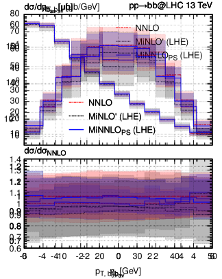
Figure 2: Validation of MiNNLO_PS predictions against NNLO QCD results. See text for details.

We start by validating the predictions of our MiNNLO_PS generator in the fully inclusive phase space of the bottom-quark pair against fixed-order NNLO results [48] from Matrix [49]. The fully inclusive MiNNLO_PS cross section for bottom-quark pair production amounts to $428.7(6)_{-11\%}^{+13\%}\,\mu b$, which is in perfect agreement with the fixed-order NNLO QCD result of $435(2)_{-15\%}^{+16\%}\,\mu b$. For a more direct comparison, the MiNNLO_PS distributions are shown here at the Les-Houches-Event (LHE) level without showering effects. Figure 2 displays three differential distributions in the kinematics of the bottom quarks namely the average rapidity ($y_{b_{\rm av}}$), pseudo-rapidity ($\eta_{b_{\rm av}}$), and transverse momentum ($p_{T,b_{\rm av}}$) of the bottom and antibottom quark. These observables are all non-trivial in the Born phase space and therefore they are genuinely NNLO QCD accurate. Besides MiNNLO_PS (blue solid) and fixed-order NNLO QCD predictions (red dashed), we also include MiNLO^′ results (black dotted) as a reference, which are NLO QCD accurate in all 0-jet (and 1-jet) observables. First of all, we see in Figure 2 that the NNLO QCD corrections included through the MiNNLO_PS procedure have an impact of $\mathcal{O}(+10\%)$ with respect to MiNLO^′. Moreover, the corrections are very flat as a function of the rapidities, while there are slight shape effects in $p_{T,b_{\rm av}}$. However, one should bear in mind that the 0-jet and 1-jet merged MiNLO^′ prediction already includes important corrections (beyond fixed-order NLO QCD) due to the NLO QCD corrections to hard parton radiation in the 1-jet phase space. When comparing MiNNLO_PS predictions with the fixed-order NNLO QCD results, we find that all observables are fully compatible within their respective perturbative uncertainties. We note that these two calculations differ by terms beyond accuracy and they are not expected to yield identical results. Despite this fact, one can see that the central predictions are extremely close and the size of the uncertainty bands is very similar. With this we conclude the validation of the NNLO QCD accuracy of the MiNNLO_PS generator and move on to considering predictions for $B$ hadron production at the LHC.

Analysis	Energy	Process	Measured cross section ($\mu b$)	MiNNLOPS ($\mu b$)
ATLAS [12]	7 TeV	$pp\rightarrow B^{+}$+$X$	$10.6\pm 0.3\text{\scriptsize(stat)}\pm 0.7\text{\scriptsize(syst)}$ $\pm 0.2\text{\scriptsize(lumi)}\pm 0.4\text{\scriptsize(bf)}$	$10.17(5)_{-14.0\%}^{+13.3\%}$
CMS [16]	13 TeV	$pp\rightarrow B^{+}$+$X$	$15.3\pm 0.4\text{\scriptsize(stat)}\pm 2.1\text{\scriptsize(syst)}\pm 0.4\text{\scriptsize(lumi)}$	$11.47(6)_{-13.2\%}^{+11.3\%}$
LHCb-1 [19]	7 TeV	$pp\rightarrow B^{\pm}$+$X$	$38.9\pm 0.3\text{\scriptsize(stat)}\pm 2.5\text{\scriptsize(syst)}\pm 1.3\text{\scriptsize(bf)}$	${42.2(1)}_{-11.4\%}^{+13.9\%}$
		$pp\rightarrow B^{0}$+$X$	$38.1\pm 0.6\text{\scriptsize(stat)}\pm 3.7\text{\scriptsize(syst)}\pm 4.7\text{\scriptsize(bf)}$	$42.3(1)_{-11.3\%}^{+14.7\%}$
		$pp\rightarrow B^{0}_{s}$+$X$	$10.5\pm 0.2\text{\scriptsize(stat)}\pm 0.8\text{\scriptsize(syst)}\pm 1.0\text{\scriptsize(bf)}$	$9.32(6)_{-11.5\%}^{+13.6\%}$
LHCb-2 [21]	7 TeV	$pp\rightarrow B^{\pm}$+$X$	$43.0\pm 0.2\text{\scriptsize(syst)}\pm 2.5\text{\scriptsize(stat)}\pm 1.7\text{\scriptsize(bf)}$	$42.2(1)_{-11.4\%}^{+13.9\%}$
	13 TeV	$pp\rightarrow B^{\pm}$+$X$	$86.6\pm 0.5\text{\scriptsize(stat)}\pm 5.4\text{\scriptsize(syst)}\pm 3.4\text{\scriptsize(bf)}$	$78.5(3)_{-9.3\%}^{+9.0\%}$
LHCb-3 [20]	7 TeV	$pp\rightarrow B$+$X$	$72.0\pm 0.3\text{\scriptsize(stat)}\pm 6.8\text{\scriptsize(syst)}$	$65.3(1)_{-10.5\%}^{+12.6\%}$
	13 TeV	$pp\rightarrow B$+$X$	$144\pm 1\text{\scriptsize(stat)}\pm 21\text{\scriptsize(syst)}$	$116.2(3)_{-12.3\%}^{+7.6\%}$

Table 1: Fiducial cross sections for the production of different $B$ hadron final states for various LHC analyses and compared against MiNNLO_PS predictions. See text for details.

First, we consider various cross-section measurements of $B$ meson (and hadron) production at different LHC energies and by different experiments in Table 1, with standard experimental uncertainties (statistical, systematical, luminosity) and one related to the assumed branching fractions (bf) of the $B$ hadrons. These analyses measure the cross section for the production of different $B$ hadrons. The ATLAS 7 TeV analysis of Ref. [12] and the CMS 13 TeV analysis of Ref. [16] select only $B^{+}$ mesons, for instance. The LHCb-1 analysis at 7 TeV [19], on the other hand, measures separately $B^{\pm}$, $B^{0}$ and $B^{0}_{s}$ meson cross sections (the latter two include also the charge conjugate mesons), while the LHCb-2 analysis [21] includes both $B^{+}$ and $B^{-}$ meson, providing their cross sections at 7 TeV and 13 TeV. Only the LHCb-3 study of Ref. [20] accounts for all relevant $B$ hadrons, including also some baryons, in order to provide predictions as close as possible to the originally produced bottom quarks. By and large, it is quite remarkable how well our MiNNLO_PS predictions agree with the measured cross sections within the quoted experimental and theoretical uncertainties, except for the CMS measurement at 13 TeV, where the MiNNLO_PS prediction is somewhat lower. Moreover, the experimental and theoretical uncertainties are largely of similar size, which shows that NNLO+PS accuracy is required, also in view of future measurements.

1	1	1	1

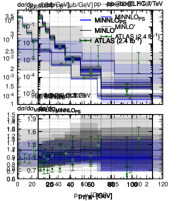
Figure 3: Comparison to ATLAS 7 TeV data [12]. See text for details.

We continue by studying our MiNNLO_PS predictions in comparison to differential measurements. In Figure 3 we consider the data (green points) from the $B^{+}$-meson analysis by ATLAS at 7 TeV for the $B^{+}$ rapidity ($y_{B^{+}}$) and transverse momentum ($p_{T,B^{+}}$). The upper figures show the two single differential distributions in the selected phase space, while the lower ones are the double differential distributions, namely the $p_{T,B^{+}}$ observable in slices of $y_{B^{+}}$. From the $y_{B^{+}}$ distribution it is clear that NNLO corrections of the MiNNLO_PS prediction (blue, solid) with respect to the MiNLO^′ result is completely flat and practically zero in this fiducial setup, while they induce a substantial reduction of the theoretical higher-order uncertainties estimated from scale variation. For the $p_{T,B^{+}}$ spectrum, on the other hand, we see that MiNNLO_PS predicts a softer behaviour in the tail of the distribution, which induces a slight improvement in the description of the data. However, in either case, both MiNLO^′ and MiNNLO_PS predictions are in full agreement with the measured $y_{B^{+}}$ and $p_{T,B^{+}}$ distributions within uncertainties. This is true, also for the double-differential $p_{T,B^{+}}$–$y_{B^{+}}$ results with the exception of a fluctuation of the data in a single bin. Overall, the picture remains the same though: MiNNLO_PS features much smaller uncertainty bands compared to MiNLO^′ , a softer $p_{T,B^{+}}$ spectrum in each $y_{B^{+}}$ slice, and a remarkable agreement with data.

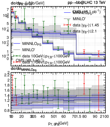
Figure 4: Comparison to CMS 13 TeV data [16]. See text for details.

Next, we present a comparison against the CMS measurement at 13 TeV of $y_{B^{+}}$ and $p_{T,B^{+}}$ in Figure 4. In this analysis, the $10\leq p_{T,B^{+}}\leq 17$ GeV region is measured with a smaller rapidity range (up to $|y|\leq 1.45$) and the extended range ($p_{T,B^{+}}\leq 100$ GeV) is measured up to $|y|\leq 2.1$, which explains the differently labelled data points. As one can see, all data points are consistently above the MiNNLO_PS predictions (despite being largely within the quoted uncertainties). We already observed this (small) discrepancy for the measured cross section in Table 1. The shape of the differential distributions, on the other hand, are well described by the MiNNLO_PS predictions.

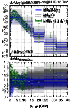
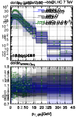
1

1

1

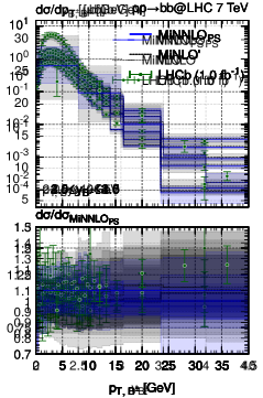
1

1

1

1

1

1

1

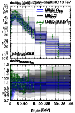
Figure 5: Comparison to LHCb data at 7 and 13 TeV [21]. See text for details.

A very similar picture as for the ATLAS 7 TeV comparison in Figure 3 emerges for the LHCb-2 $B^{\pm}$ data at 7 TeV and 13 TeV in Figure 5, which shows the rapidity ($y_{B^{\pm}}$) and transverse momentum ($p_{T,B^{\pm}}$) of the $B^{\pm}$ mesons. One should notice that due to their asymmetric detector design LHCb can measure only in one rapidity direction, but up to significantly larger values of it. Moreover, the LHCb-2 exhibits a very fine binning in $p_{T,B^{\pm}}$. Once again, we observe an extremely good agreement with the MiNNLO_PS predictions. This is is true not only in terms of normalization, but also in terms of the shapes, especially for the finely binned $p_{T,B^{\pm}}$ distribution.

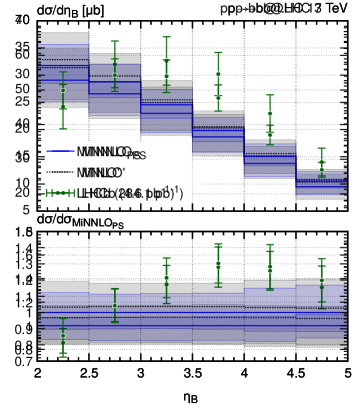
Figure 6: Comparison to LHCb rapidity distributions at 7 and 13 TeV [20]. See text for details.

In Figure 6 we show results for the LHCb-3 analysis for the pseudorapidity of the $B$ hadron ($\eta_{B}$), which includes all relevant $B$ hadrons that yield a sufficiently large contribution to the cross section. In this case, the $\eta_{B}$ shape, especially of the 13 TeV measurement, cannot be reproduced by our predictions. This is in line with the fact that neither the FONLL result quoted in this analysis [20] nor the recent NNLO QCD calculation [48] predict such a shape. Given that all other rapidity measurements are in excellent agreement with SM predictions, especially those presented here from our MiNNLO_PS generator, it seems unlikely that this is induced by some new-physics phenomenon.

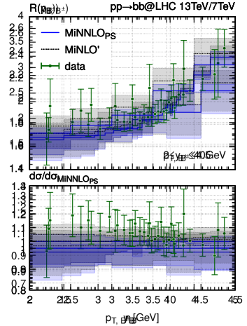
Figure 7: Comparison to 13 TeV/7 TeV ratios measured by LHCb [21, 20]. See text for details.

Finally, we briefly comment on the 13 TeV/7 TeV ratios presented in the LHCb-2 analysis for the $p_{T,B^{\pm}}$ and $y_{B^{\pm}}$ distributions, and in the LHCb-3 analysis for the $\eta_{B}$ distribution, shown in Figure 7. In all cases, the MiNNLO_PS corrections are quite small ($\sim-5\%$) and flat in each distribution. Moreover, the scale uncertainties are reduced to the $\sim 10\%$ level and slightly smaller for MiNNLO_PS compared to MiNLO^′. The experimental data is full agreement with the predictions.

4 Summary

To summarize, we have presented a fully exclusive simulation of $B$ hadron production at the LHC, which describes the underlying hard process $pp\to b\bar{b}$ at NNLO QCD accuracy. We have validated the accuracy of our NNLO+PS calculation for bottom-quark pair production against fixed-order NNLO QCD predictions. The comparison to LHC data from various analyses by ATLAS, CMS and LHCb at 7 and/or 13 TeV shows that the NNLO QCD corrections are important to reach an accurate description of $B$ meson (and $B$ hadron) observables. Not only do we find very good agreement of our MiNNLO_PS predictions with data both at the cross-section and at the distribution level, we also observe a clear reduction of uncertainties with respect to lower order predictions. We reckon that our new $b\bar{b}$ MiNNLO_PS generator, which can be used to simulate fully exclusively the kinematics of the bottom-flavoured hadronic final states, will be particularly useful for future $B$ hadron measurements at the LHC. The code will be made publicly available within the Powheg-Box-Res framework.

Our calculation allows us to have an accurate and realistic description of $b$-jet cross sections as well, enabling a direct comparison to $b$-jet measurements at the LHC. In this context, also the impact of different algorithms to define the jet flavour [83, 84, 85, 86, 87, 88, 89, 90, 91] can be studied, which received quite some attention recently. We leave such studies to future work.

Acknowledgements. We would like to thank Pier Francesco Monni, Paolo Nason and Emanuele Re for comments on the manuscript. We have used the Max Planck Computing and Data Facility (MPCDF) in Garching to carry out all simulations presented here.

References

- Albajar et al. [1987] C. Albajar et al. (UA1), Phys. Lett. B 186, 237 (1987).
- Albajar et al. [1988] C. Albajar et al. (UA1), Phys. Lett. B 213, 405 (1988).
- Abe et al. [1995] F. Abe et al. (CDF), Phys. Rev. Lett. 75, 1451 (1995), arXiv:hep-ex/9503013.
- Acosta et al. [2002] D. Acosta et al. (CDF), Phys. Rev. D 65, 052005 (2002), arXiv:hep-ph/0111359.
- Acosta et al. [2005] D. Acosta et al. (CDF), Phys. Rev. D 71, 032001 (2005), arXiv:hep-ex/0412071.
- Abulencia et al. [2007] A. Abulencia et al. (CDF), Phys. Rev. D 75, 012010 (2007), arXiv:hep-ex/0612015.
- Abachi et al. [1995] S. Abachi et al. (D0), Phys. Rev. Lett. 74, 3548 (1995).
- Abbott et al. [2000] B. Abbott et al. (D0), Phys. Lett. B 487, 264 (2000), arXiv:hep-ex/9905024.
- Abelev et al. [2014] B. B. Abelev et al. (ALICE), Phys. Lett. B 738, 97 (2014), arXiv:1405.4144 [nucl-ex].
- Abelev et al. [2013] B. Abelev et al. (ALICE), Phys. Lett. B 721, 13 (2013), [Erratum: Phys.Lett.B 763, 507–509 (2016)], arXiv:1208.1902 [hep-ex].
- Aad et al. [2012] G. Aad et al. (ATLAS), Nucl. Phys. B 864, 341 (2012), arXiv:1206.3122 [hep-ex].
- Aad et al. [2013] G. Aad et al. (ATLAS), JHEP 10, 042 (2013), arXiv:1307.0126 [hep-ex].
- Khachatryan et al. [2011] V. Khachatryan et al. (CMS), Phys. Rev. Lett. 106, 112001 (2011), arXiv:1101.0131 [hep-ex].
- Chatrchyan et al. [2011] S. Chatrchyan et al. (CMS), Phys. Rev. Lett. 106, 252001 (2011), arXiv:1104.2892 [hep-ex].
- Chatrchyan et al. [2012] S. Chatrchyan et al. (CMS), JHEP 06, 110 (2012), arXiv:1203.3458 [hep-ex].
- Khachatryan et al. [2017] V. Khachatryan et al. (CMS), Phys. Lett. B 771, 435 (2017), arXiv:1609.00873 [hep-ex].
- Aaij et al. [2010] R. Aaij et al. (LHCb), Phys. Lett. B 694, 209 (2010), arXiv:1009.2731 [hep-ex].
- Aaij et al. [2012] R. Aaij et al. (LHCb), JHEP 04, 093 (2012), arXiv:1202.4812 [hep-ex].
- Aaij et al. [2013] R. Aaij et al. (LHCb), JHEP 08, 117 (2013), arXiv:1306.3663 [hep-ex].
- Aaij et al. [2017a] R. Aaij et al. (LHCb), Phys. Rev. Lett. 118, 052002 (2017a), [Erratum: Phys.Rev.Lett. 119, 169901 (2017)], arXiv:1612.05140 [hep-ex].
- Aaij et al. [2017b] R. Aaij et al. (LHCb), JHEP 12, 026 (2017b), arXiv:1710.04921 [hep-ex].
- Nason et al. [1988] P. Nason, S. Dawson and R. K. Ellis, Nucl. Phys. B 303, 607 (1988).
- Nason et al. [1989] P. Nason, S. Dawson and R. K. Ellis, Nucl. Phys. B 327, 49 (1989), [Erratum: Nucl.Phys.B 335, 260–260 (1990)].
- Beenakker et al. [1989] W. Beenakker, H. Kuijf, W. L. van Neerven and J. Smith, Phys. Rev. D 40, 54 (1989).
- Mangano et al. [1992] M. L. Mangano, P. Nason and G. Ridolfi, Nucl. Phys. B 373, 295 (1992).
- Garzelli et al. [2021] M. V. Garzelli, L. Kemmler, S. Moch and O. Zenaiev, JHEP 04, 043 (2021), arXiv:2009.07763 [hep-ph].
- Cacciari and Greco [1994] M. Cacciari and M. Greco, Nucl. Phys. B 421, 530 (1994), arXiv:hep-ph/9311260.
- Mele and Nason [1991] B. Mele and P. Nason, Nucl. Phys. B 361, 626 (1991), [Erratum: Nucl.Phys.B 921, 841–842 (2017)].
- Cacciari and Catani [2001] M. Cacciari and S. Catani, Nucl. Phys. B 617, 253 (2001), arXiv:hep-ph/0107138.
- Kniehl et al. [2005a] B. A. Kniehl, G. Kramer, I. Schienbein and H. Spiesberger, Phys. Rev. D 71, 014018 (2005a), arXiv:hep-ph/0410289.
- Kniehl et al. [2005b] B. A. Kniehl, G. Kramer, I. Schienbein and H. Spiesberger, Eur. Phys. J. C 41, 199 (2005b), arXiv:hep-ph/0502194.
- Kramer and Spiesberger [2018] G. Kramer and H. Spiesberger, Phys. Rev. D 98, 114010 (2018), arXiv:1809.04297 [hep-ph].
- Benzke et al. [2019] M. Benzke, B. A. Kniehl, G. Kramer, I. Schienbein and H. Spiesberger, Eur. Phys. J. C 79, 814 (2019), arXiv:1907.12456 [hep-ph].
- Cacciari et al. [1998] M. Cacciari, M. Greco and P. Nason, JHEP 05, 007 (1998), arXiv:hep-ph/9803400.
- Cacciari et al. [2001] M. Cacciari, S. Frixione and P. Nason, JHEP 03, 006 (2001), arXiv:hep-ph/0102134.
- Cacciari and Nason [2002] M. Cacciari and P. Nason, Phys. Rev. Lett. 89, 122003 (2002), arXiv:hep-ph/0204025.
- Cacciari et al. [2012] M. Cacciari, S. Frixione, N. Houdeau, M. L. Mangano, P. Nason and G. Ridolfi, JHEP 10, 137 (2012), arXiv:1205.6344 [hep-ph].
- Cacciari et al. [2006] M. Cacciari, P. Nason and C. Oleari, JHEP 04, 006 (2006), arXiv:hep-ph/0510032.
- Kartvelishvili et al. [1978] V. G. Kartvelishvili, A. K. Likhoded and V. A. Petrov, Phys. Lett. B 78, 615 (1978).
- Peterson et al. [1983] C. Peterson, D. Schlatter, I. Schmitt and P. M. Zerwas, Phys. Rev. D 27, 105 (1983).
- Frixione et al. [2007a] S. Frixione, P. Nason and G. Ridolfi, JHEP 09, 126 (2007a), arXiv:0707.3088 [hep-ph].
- Buonocore et al. [2018] L. Buonocore, P. Nason and F. Tramontano, Eur. Phys. J. C 78, 151 (2018), arXiv:1711.06281 [hep-ph].
- Alwall et al. [2014] J. Alwall, R. Frederix, S. Frixione, V. Hirschi, F. Maltoni, O. Mattelaer, H. S. Shao, T. Stelzer, P. Torrielli and M. Zaro, JHEP 07, 079 (2014), arXiv:1405.0301 [hep-ph].
- Mangano et al. [2016] M. L. Mangano et al., (2016), 10.23731/CYRM-2017-003.1, arXiv:1607.01831 [hep-ph].
- d’Enterria and Snigirev [2017] D. d’Enterria and A. M. Snigirev, Phys. Rev. Lett. 118, 122001 (2017), arXiv:1612.05582 [hep-ph].
- Langenfeld et al. [2009] U. Langenfeld, S. Moch and P. Uwer, Phys. Rev. D 80, 054009 (2009), arXiv:0906.5273 [hep-ph].
- Aliev et al. [2011] M. Aliev, H. Lacker, U. Langenfeld, S. Moch, P. Uwer and M. Wiedermann, Comput. Phys. Commun. 182, 1034 (2011), arXiv:1007.1327 [hep-ph].
- Catani et al. [2021] S. Catani, S. Devoto, M. Grazzini, S. Kallweit and J. Mazzitelli, JHEP 03, 029 (2021), arXiv:2010.11906 [hep-ph].
- Grazzini et al. [2018] M. Grazzini, S. Kallweit and M. Wiesemann, Eur. Phys. J. C78, 537 (2018), arXiv:1711.06631 [hep-ph].
- Czakon et al. [2021] M. L. Czakon, T. Generet, A. Mitov and R. Poncelet, JHEP 10, 216 (2021), arXiv:2102.08267 [hep-ph].
- Mazzitelli et al. [2021] J. Mazzitelli, P. F. Monni, P. Nason, E. Re, M. Wiesemann and G. Zanderighi, Phys. Rev. Lett. 127, 062001 (2021), arXiv:2012.14267 [hep-ph].
- Mazzitelli et al. [2022] J. Mazzitelli, P. F. Monni, P. Nason, E. Re, M. Wiesemann and G. Zanderighi, JHEP 04, 079 (2022), arXiv:2112.12135 [hep-ph].
- Monni et al. [2020a] P. F. Monni, P. Nason, E. Re, M. Wiesemann and G. Zanderighi, JHEP 05, 143 (2020a), arXiv:1908.06987 [hep-ph].
- Monni et al. [2020b] P. F. Monni, E. Re and M. Wiesemann, Eur. Phys. J. C 80, 1075 (2020b), arXiv:2006.04133 [hep-ph].
- Lombardi et al. [2021a] D. Lombardi, M. Wiesemann and G. Zanderighi, JHEP 06, 095 (2021a), arXiv:2010.10478 [hep-ph].
- Lombardi et al. [2021b] D. Lombardi, M. Wiesemann and G. Zanderighi, JHEP 11, 230 (2021b), arXiv:2103.12077 [hep-ph].
- Buonocore et al. [2022] L. Buonocore, G. Koole, D. Lombardi, L. Rottoli, M. Wiesemann and G. Zanderighi, JHEP 01, 072 (2022), arXiv:2108.05337 [hep-ph].
- Lombardi et al. [2022] D. Lombardi, M. Wiesemann and G. Zanderighi, Phys. Lett. B 824, 136846 (2022), arXiv:2108.11315 [hep-ph].
- Zanoli et al. [2022] S. Zanoli, M. Chiesa, E. Re, M. Wiesemann and G. Zanderighi, JHEP 07, 008 (2022), arXiv:2112.04168 [hep-ph].
- Gavardi et al. [2022] A. Gavardi, C. Oleari and E. Re, JHEP 09, 061 (2022), arXiv:2204.12602 [hep-ph].
- Haisch et al. [2022] U. Haisch, D. J. Scott, M. Wiesemann, G. Zanderighi and S. Zanoli, JHEP 07, 054 (2022), arXiv:2204.00663 [hep-ph].
- Lindert et al. [2022] J. M. Lindert, D. Lombardi, M. Wiesemann, G. Zanderighi and S. Zanoli, JHEP 11, 036 (2022), arXiv:2208.12660 [hep-ph].
- Zhu et al. [2013] H. X. Zhu, C. S. Li, H. T. Li, D. Y. Shao and L. L. Yang, Phys. Rev. Lett. 110, 082001 (2013), arXiv:1208.5774 [hep-ph].
- Li et al. [2013] H. T. Li, C. S. Li, D. Y. Shao, L. L. Yang and H. X. Zhu, Phys. Rev. D 88, 074004 (2013), arXiv:1307.2464 [hep-ph].
- Catani et al. [2014] S. Catani, M. Grazzini and A. Torre, Nucl. Phys. B890, 518 (2014), arXiv:1408.4564 [hep-ph].
- Catani et al. [2018] S. Catani, M. Grazzini and H. Sargsyan, JHEP 11, 061 (2018), arXiv:1806.01601 [hep-ph].
- Catani et al. [2023] S. Catani, S. Devoto, M. Grazzini and J. Mazzitelli, (2023), arXiv:2301.11786 [hep-ph].
- Nason [2004] P. Nason, JHEP 11, 040 (2004), arXiv:hep-ph/0409146 [hep-ph].
- Nason and Ridolfi [2006] P. Nason and G. Ridolfi, JHEP 08, 077 (2006), arXiv:hep-ph/0606275 [hep-ph].
- Frixione et al. [2007b] S. Frixione, P. Nason and C. Oleari, JHEP 11, 070 (2007b), arXiv:0709.2092 [hep-ph].
- Alioli et al. [2010] S. Alioli, P. Nason, C. Oleari and E. Re, JHEP 06, 043 (2010), arXiv:1002.2581 [hep-ph].
- Ježo and Nason [2015] T. Ježo and P. Nason, JHEP 12, 065 (2015), arXiv:1509.09071 [hep-ph].
- Cascioli et al. [2012] F. Cascioli, P. Maierhöfer and S. Pozzorini, Phys. Rev. Lett. 108, 111601 (2012), arXiv:1111.5206 [hep-ph].
- Buccioni et al. [2018] F. Buccioni, S. Pozzorini and M. Zoller, Eur. Phys. J. C78, 70 (2018), arXiv:1710.11452 [hep-ph].
- Buccioni et al. [2019] F. Buccioni, J.-N. Lang, J. M. Lindert, P. Maierhöfer, S. Pozzorini, H. Zhang and M. F. Zoller, Eur. Phys. J. C 79, 866 (2019), arXiv:1907.13071 [hep-ph].
- Ježo et al. [2016] T. Ježo, J. M. Lindert, P. Nason, C. Oleari and S. Pozzorini, Eur. Phys. J. C 76, 691 (2016), arXiv:1607.04538 [hep-ph].
- Bärnreuther et al. [2014] P. Bärnreuther, M. Czakon and P. Fiedler, JHEP 02, 078 (2014), arXiv:1312.6279 [hep-ph].
- Ball et al. [2017] R. D. Ball et al. (NNPDF), Eur. Phys. J. C77, 663 (2017), arXiv:1706.00428 [hep-ph].
- Buckley et al. [2015] A. Buckley, J. Ferrando, S. Lloyd, K. Nordström, B. Page, M. Rüfenacht, M. Schönherr and G. Watt, Eur. Phys. J. C75, 132 (2015), arXiv:1412.7420 [hep-ph].
- Salam and Rojo [2009] G. P. Salam and J. Rojo, Comput. Phys. Commun. 180, 120 (2009), arXiv:0804.3755 [hep-ph].
- Sjöstrand et al. [2015] T. Sjöstrand, S. Ask, J. R. Christiansen, R. Corke, N. Desai, P. Ilten, S. Mrenna, S. Prestel, C. O. Rasmussen and P. Z. Skands, Comput. Phys. Commun. 191, 159 (2015), arXiv:1410.3012 [hep-ph].
- Skands et al. [2014] P. Skands, S. Carrazza and J. Rojo, Eur. Phys. J. C 74, 3024 (2014), arXiv:1404.5630 [hep-ph].
- Banfi et al. [2006] A. Banfi, G. P. Salam and G. Zanderighi, Eur. Phys. J. C 47, 113 (2006), arXiv:hep-ph/0601139.
- Buckley and Pollard [2016] A. Buckley and C. Pollard, Eur. Phys. J. C 76, 71 (2016), arXiv:1507.00508 [hep-ph].
- Ilten et al. [2017] P. Ilten, N. L. Rodd, J. Thaler and M. Williams, Phys. Rev. D 96, 054019 (2017), arXiv:1702.02947 [hep-ph].
- Caletti et al. [2021] S. Caletti, O. Fedkevych, S. Marzani, D. Reichelt, S. Schumann, G. Soyez and V. Theeuwes, JHEP 07, 076 (2021), arXiv:2104.06920 [hep-ph].
- Fedkevych et al. [2022] O. Fedkevych, C. K. Khosa, S. Marzani and F. Sforza, (2022), arXiv:2202.05082 [hep-ph].
- Caletti et al. [2022a] S. Caletti, A. J. Larkoski, S. Marzani and D. Reichelt, Eur. Phys. J. C 82, 632 (2022a), arXiv:2205.01109 [hep-ph].
- Caletti et al. [2022b] S. Caletti, A. J. Larkoski, S. Marzani and D. Reichelt, JHEP 10, 158 (2022b), arXiv:2205.01117 [hep-ph].
- Czakon et al. [2022] M. Czakon, A. Mitov and R. Poncelet, (2022), arXiv:2205.11879 [hep-ph].
- Gauld et al. [2022] R. Gauld, A. Huss and G. Stagnitto, (2022), arXiv:2208.11138 [hep-ph].