SegForestNet: Spatial-Partitioning-Based Aerial Image Segmentation

Abstract

Aerial image analysis, specifically the semantic segmentation thereof, is the basis for applications such as automatically creating and updating maps, tracking city growth, or tracking deforestation. In true orthophotos, which are often used in these applications, many objects and regions can be approximated well by polygons. However, this fact is rarely exploited by state-of-the-art semantic segmentation models. Instead, most models allow unnecessary degrees of freedom in their predictions by allowing arbitrary region shapes. We therefore present a refinement of our deep learning model which predicts binary space partitioning trees, an efficient polygon representation. The refinements include a new feature decoder architecture and a new differentiable BSP tree renderer which both avoid vanishing gradients. Additionally, we designed a novel loss function specifically designed to improve the spatial partitioning defined by the predicted trees. Furthermore, our expanded model can predict multiple trees at once and thus can predict class-specific segmentations. Taking all modifications together, our model achieves state-of-the-art performance while using up to 60% fewer model parameters when using a small backbone model or up to 20% fewer model parameters when using a large backbone model.

1 Introduction

Computer vision techniques, such as object detection and semantic segmentation, are used for many aerial image analysis applications. As an example, traffic can be analyzed by using object detection to find vehicles in aerial images. Semantic segmentation is the basis for creating and updating maps [11] and can be used for tracking city growth [13] or tracking deforestation [23].

However, any error in the prediction of a computer vision model, i.e., object detection or semantic segmentation, causes errors in applications based on said prediction. Precise predictions are required, which can be achieved by exploiting domain knowledge. One fact rarely exploited in the deep learning-based analysis of aerial images is that many objects and regions can be approximated well by polygons, especially in true orthophotos. By restricting a model’s prediction to a limited number of polygons, the degrees of freedom in the prediction are reduced. Arbitrary region shapes, e.g., circle-shaped cars which make no sense, are no longer feasible predictions.

We created BSPSegNet[14], a model for aerial image segmentation which predicts polygons as shown in Fig. 1. The model partitions the input image into $8\times 8$ blocks. For each block, a binary space partitioning (BSP) tree [10] with depth 2 is predicted, i.e., every block is partitioned into up to four segments with a separate class prediction for each segment. The parameters of the inner nodes of the BSP tree encode parameters of a line partitioning a region into two subregions, while the parameters of the leaf nodes are class logits. The lines encoded by the inner nodes together with the block boundaries form polygons. As we demonstrated in our earlier paper, the ground truth of common aerial image datasets can be encoded extremely accurately this way ($99\%$ accuracy and $99\%$ mean Intersection-over-Union (mIoU)).

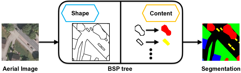
Figure 1: Overview of our approach: our model predicts binary space partitioning (BSP) trees from aerial images. The inner nodes of such a tree define the shape of regions, while the leaf nodes define the content of each region. The leaf nodes effectively map shapes to classes. BSP trees can be rendered in a differentiable way into a full segmentation thus enabling end-to-end model training. Our proposed refinements improve gradient computations in the BSP renderer and parts of the model. Additionally, a novel loss function improves the predicted inner node parameters, i.e., the predicted shapes. Furthermore, we extended the approach to predict multiple trees at the same time in order to enable class-specific shape predictions.

However, despite reaching state-of-the-art performance in semantic segmentation, BSPSegNet still does not offer proven improvements over existing models. In this article, we aim to improve BSPSegNet such that it performs better than the state-of-the-art for segmentation. We present multiple contributions:

1. We replace BSPSegNet’s two feature decoders with an architecture using residual connections and modify the model’s differentiable BSP tree renderer to avoid using sigmoid activations. BSPSegNet tries to push the output of these activations close to $0$ or $1$. However, in these value regions the derivative of the sigmoid function is almost $0$. Vanishing gradients are avoided due to these modifications.

2. We introduce a novel loss function punishing BSP trees which create partitions containing multiple different classes (according to the ground truth). This loss specifically affects only the inner nodes of the BSP trees, instead of all the nodes as categorical cross entropy does, thus improving the shapes of the predicted partitions.

3. We expand BSPSegNet’s prediction s.t. it is able to predict multiple BSP trees for each $8\times 8$ block, thus enabling class-specific segmentations for more precise shape predictions.

Due to the last modification, we rename our model to SegForestNet. SegForestNet is able to reach state-of-the-art performance while using up to $60\%$ less parameters, i.e., it is less prone to overfitting to a small dataset. Small dataset size is a common problem in aerial image analysis.

With these modifications SegForestNet can be trained end-to-end without the two phase training previously recommended in [14]. In the first phase, an autoencoder phase, a mapping of the ground truth to BSP trees was learned. In the second phase, this new ground truth representation was used to learn the actual semantic segmentation without using the differentiable BSP renderer and thus avoiding its effects on gradients. Our modifications allow the faster and more efficient training of SegForestNet without the autoencoder phase.

In addition to the above contributions, we also experimented with different signed distance functions (SDFs) and tree structures. SDFs are used by the inner node nodes in order to partition a segment into subsegments. By trying different SDFs, we were able to generalize the shape of the partitioning boundary from lines to other shapes such as circles. Also, our approach generalizes to different tree structures such as quadtrees [9] and k-d trees [1]. However, we found that neither of these two changes provide any benefit for the semantic segmentation of aerial images. Since we believe that these ideas may be useful in other domains with more organic shapes, e.g., the segmentation of images captured by cameras of self-driving cars, we still present these experiments here so that they become more easily reproducible.

In this article’s next section we will discuss related work, followed by a description of SegForestNet. We then evaluate our contributions by comparing SegForestNet on several datasets to multiple state-of-the-art semantic segmentation models. We finally conclude with a summary.

Our implementation can be found on GitHub.

2 Related Work

Modern semantic segmentation models rely on deep learning and an encoder-decoder structure [30, 49, 19, 3, 43, 31]. An encoder is used to map an input image to a feature map with a reduced spatial resolution but a much higher number of channels/features. While a large number of features is computed, the spatial information is bottlenecked. This implies that downsampling, e.g., through max-pooling or strided convolutions, is performed. Using such a feature map, a decoder predicts the desired semantic segmentation. To get a segmentation of the same resolution as the input image, the decoder uses bilinear sampling and/or transpose convolutions (also called deconvolutions) in order to upsample the spatial resolution of the feature map back to the initial input resolution.

U-Net [32] is a popular model following this paradigm. Though designed for medical image analysis, it is also used for other types of data, including even 3D data [7]. U-Net’s encoder and decoder are almost symmetrical and skip connections at each spatial resolution are used to allow predictions with high frequency details. Other models, such as Fully Convolutional Networks for Semantic Segmentation (FCN) [25], have an asymmetrical architecture with a significantly more sophisticated encoder than decoder. They rely on existing classification models, such as VGG [37], ResNet [16], MobileNetv2 [35] or Xception [6], as encoder (also called backbone or feature extractors in these cases) by removing the final classification layers. Instead, semantic segmentation models append a novel decoder to these encoders. The complexity of these decoders varies. While FCN uses a rather simple decoder, DeepLabv3+ [4] uses a more sophisticated decoder and also adds atrous spatial pyramid pooling [2] to the encoder. By doing so, DeepLabv3+ is able to account for context information at different scales. Other modifications to the basic encoder-decoder idea are adding parallel branches to process specific features such as edges/boundaries [39], processing videos instead of images [52], explicitly modelling long-range spatial and channel relations [29], separating the image into fore- and background [50], or point-wise affinity propagation to handle imbalanced class distributions with an unusually high number of background pixels [24].

More recent research also works on more complex problems, e.g., instance segmentation [15] and panoptic segmentation [21, 45, 47, 48]. In instance segmentation pixel masks of detected objects, such as cars or persons, are predicted. Panoptic segmentation is a combination of semantic segmentation and instance segmentation: a class is predicted for each pixel in the input image while for all pixels of countable objects an additional instance ID is predicted. Models dealing with these more complex tasks still usually require a semantic segmentation as a component to compute the final prediction. AdaptIS [38] is such a model. When performing instance segmentation, it uses U-Net as a backbone while using ResNet and DeepLabv3+ when performing panoptic segmentation.

Our previous model, BSPSegNet [14], predicts BSP trees to perform a semantic segmentation. These trees are usually used in computer graphics [36] rather than computer vision. Each inner node of a BSP tree partitions a given region into two segments while the leaf nodes define each segment’s content, i.e., its class in the case of a semantic segmentation. Since BSP trees are resolution-indepedent, BSPSegNet’s decoder does not have to perform any kind of upsampling. Furthermore, BSPSSegNet is the only segmentation model which inherently semantically separates features into shape and content features. Similar works using computer graphics techniques for computer vision are PointRend [22] and models reconstructing 3D meshes [40, 41, 28, 12]. PointRend iteratively refines a coarse instance segmentation into a finer representation. BSPnet [5] also uses BSP, but instead of a segmentation, it tries to reconstruct polygonal 3D models. Additionally, rather than predicting a BSP tree hierarchy, it instead predicts a set of BSP planes.

As mentioned before, BSP trees are a data structure more common in computer graphics than in computer vision. Other commonly used data structures in computer graphics and other applications, e.g., data compression, are $k$-d trees [1], quadtrees [9], and bounding volume hierarchies [8]. They differ from BSP trees in that they perform a partitioning using an axis-aligned structure which makes slopes expensive to encode compared to BSP trees.

3 Semantic Segmentation through Spatial Partitioning

We will first briefly describe BSPSegNet’s architecture in this section in order to be able to precisely discuss our contributions. The third subsection presents the first contribution mentioned in the introduction, which reduces the risk of vanishing gradients, while the fourth subsection presents our second contribution, the novel loss function. The fifth subsection then discusses the changes necessary to enable to the prediction of multiple partitioning trees simultaneously, our third contribution. In a final subsection we show how SegForestNet’s differentiable BSP rendering generalizes to different signed distance functions (SDFs) and tree structures.

3.1 BSPSegNet

Fig. 2 (top) shows a common encoder-decoder architecture used by state-of-the-art models. An encoder maps an input image to a feature map with a bottlenecked spatial resolution. This feature map is then decoded into a semantic segmentation at the same spatial resolution as the input image. Skip connections at different spatial resolutions help to maintain high frequency details.

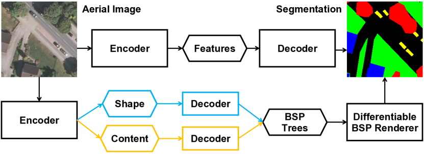
Figure 2: A comparison of state-of-the-art models (top) and BSPSegNet/SegForestNet (bottom; ours). All models use an encoder-decoder architecture, however, our models semantically splits the feature map (hexagon) into shape and content features. These are decoded into the inner nodes and leaf nodes of BSP trees respectively (see Fig. 3). Our models also needs a differentiable BSP renderer to enable end-to-end training. The renderer is a fixed function without learnable parameters.

The bottom of Fig. 2 shows BSPSegNet in comparison. As other state-of-the-art models, it uses an encoder-decoder architecture. However, it uses two separate decoders. The feature map computed by the encoder is split along the feature dimension into two separate maps: one for shape features (blue) and one for content features (orange). Each feature map is processed by a different decoder. While the decoders share the same architecture, they both have their own unique weights. The shape features are decoded into the inner nodes of the BSP trees, which represent the shape of the regions in the final segmentation, as shown in Fig. 3. The content features are decoded into the leaf nodes of the BSP trees, which represent each region’s class logits.

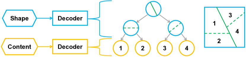
Figure 3: A partitioning of a square region (right) defined by a BSP tree (center). Shape features are decoded into the parameters of the inner nodes (blue), which define lines (green) creating the partitioning. Content features are decoded into the parameters of the leaf nodes (orange), which are the class logits predicted for each partition.

Like in other semantic segmenation models, BSPSegNet uses the feature extraction part of a classification model like MobileNetv2 or Xception as an encoder. By removing pooling operations or reducing the stride of convolution operations, the encoder is modified such that the input image is downsampled by a factor of $8$ along each spatial dimension. To keep in line with classification model design, the earlier downsampling operations are kept while the later ones are removed. This enables more efficient inference and training, as the spatial resolution is reduced early. Furthermore, the number of features in the final feature map computed by the encoder is reduced such that there is a bottleneck. The shape feature map has fewer features than the number of parameters required for the inner nodes, while the content feature map has fewer features than the parameters required for the leaf nodes.

BSPSegNet subdivides the input image into $8\times 8$ blocks (the same as the downsampling factor in the encoder) and predicts a separate BSP tree for each block, i.e., the spatial resolution of the feature map is such that there is exactly one spatial unit per block. The two decoders keep the spatial resolution and only modify the number of features. This is done by concatenating three blocks, each consisting of a $1\times 1$ convolution outputting $256$ features, batch normalization and a LeakyReLU activation. These blocks are followed by one final $1\times 1$ convolution to predict the final BSP tree parameters.

3.2 BSPSegNet’s Differentiable BSP Renderer

The differentiable BSP renderer is based on the idea of a region map R. For each pixel $\textbf{p}=(x,y)$, the entry $\textbf{R}_{iyx}$ is the probability that p is part of the $i$-th region (leaf node). This implies $\sum_{i=1}^{k}\textbf{R}_{iyx}=1$ for all pixels p with $k$ equal to the number of leaf nodes.

Initially, BSPSegNet starts with all $\textbf{R}_{iyx}$ set to $1$ and then updates the region map for every inner node. Each inner node consists of three parameters, two parameters for the normal vector n and one parameter $d$. These parameters together define a line in the two-dimensional image space. BSPSegNet does neither normalize n, nor does it enforce $|\textbf{n}|=1$ through any kind of loss. Rather, it lets the network learn to predict an appropriately scaled $d$. For every inner node and pixel p, the signed distance function $f(\textbf{p})=\textbf{n}\cdot\textbf{p}-d$ is computed. The equations

$$g(\textbf{p})=\sigma(\lambda_{1}\cdot f(\textbf{p}))$$ (1)

$$\textbf{R}_{iyx}:=\textbf{R}_{iyx}\cdot\lambda_{2}\cdot g(\textbf{p})$$ (2)

$$\textbf{R}_{iyx}:=\textbf{R}_{iyx}\cdot\lambda_{2}\cdot(1-g(\textbf{p}))$$ (3)

with the sigmoid function $\sigma$ are then used to update the region map R. For each inner node, equation 2 is used for all leaf nodes $i$ reachable from the left child node while equation 3 is used for all $i$ reachable by the right child node.

Depending on where the pixel p lies, the function $g$ either approaches $0$ or $1$. It approaches $1$ if p is reachable via the left child node and it approaches $0$ if p is reachable via the right child node. Therefore, $\textbf{R}_{iyx}$ is multiplied with a value close to $0$ for those regions $i$ which p does not belong to. Thus, eventually, all $\textbf{R}_{iyx}$ for $i$ to which p does not belong will be close to $0$. The one remaining entry $\textbf{R}_{iyx}$ will be close to $\lambda_{2}^{D}$, where $D$ is the depth of the BSP tree.

After iterating over all inner nodes, a Softmax operation across the region dimension $i$ is applied. This ensures that each $\textbf{R}_{iyx}$ represents the aforementioned probability. The hyperparameter $\lambda_{2}$ controls how close the respective final entries of R will be to $0$ or $1$, while $\lambda_{1}$ controls how large $|f(\textbf{p})|$ must be in order for p to be assigned to one specific child node ($g(\textbf{p})$ close to $0$ or $1$) instead of the model expressing uncertainty about which child region p belongs to ($g(\textbf{p})\approx 0.5$).

The final output $h$ of the BSP renderer is

$$h(\textbf{p})=\sum_{i=1}^{k}\textbf{R}_{iyx}\cdot\textbf{v}_{i}$$ (4)

with the vectors $\textbf{v}_{i}$ of class logits, one vector for each leaf node. The function $h$ can be computed in parallel for all pixels p. BSP trees are resolution-independent, therefore the final output resolution is determined by how densely $h$ is sampled, i.e., for how many pixels p the function is computed. This is also the reason why BSPSegNet, in contrast to other segmentation models, does not have to perform any kind of upsampling in its decoders. By sampling $h$ at the same resolution as the input image, a pixelwise semantic segmentation can be computed like for any other state-of-the-art model.

3.3 Refined Gradients

As mentioned in the introduction, a two-phase training process is recommended for the original BSPSegNet. In the second phase, the differentiable BSP renderer is skipped altogether. We hypothesize that insufficient gradients are responsible: by pushing the computation of $g$ (Eq. 1) into value ranges where its derivative is almost $0$ gradients vanish. Additionally, the two feature decoders do not use residual connections, which would help gradients to propagate through the model. Our first contribution aims to improve on these two points in order to avoid the two-phase training process and to enable the use of decoders with more layers which can learn more complex mapping functions from features to BSP tree parameters. The goal is to enable true end-to-end training without the need to learn a mapping to an intermediate representation. This way, training is faster, allowing for more iterations during development, e.g., for hyperparameter optimization, or saving energy and thus reducing costs.

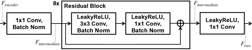
Figure 4: Our refined decoder architecture using residual blocks. The initial and the last convolution change the number of features $F$. The number of features are set such that there is a bottleneck with regard to the tree parameters, i.e., $F_{encoder}<F_{tree}$.

The first part of this contribution is a new feature decoder architecture. Again, we use the same architecture for both decoders, but they still do not share weights. Our new architecture, shown in Fig. 4, starts and ends with a $1\times 1$ convolution, the first one maps the bottlenecked feature dimension coming from the encoder to an intermediate number of features, while the last convolution maps the intermediate features to the final number of tree parameters. In between these two convolutions are several residual blocks. Each block consists of a depthwise $3\times 3$ convolution with zero padding and a $1\times 1$ convolution. The number of features stays constant throughout the residual blocks. Each convolution in the decoders, except for the very last one mapping to the tree parameters, is followed by a batch normalization layer [17] and a LeakyReLU activation [46]. This architecture not only uses residual connections for improved gradient propagation, but it also includes spatial context for each block, i.e., for each BSP tree, instead of solely relying on the receptive field of the encoder.

The second part of our first contribution is an updated region map R computation (Eqs. 1-3). We start by setting all $\textbf{R}_{iyx}$ to $0$ initially instead of $1$. For each inner node, we use the equations

$$g(\textbf{p})=\lambda\cdot f(\textbf{p})$$ (5)

$$\textbf{R}_{iyx}:=\textbf{R}_{iyx}+\text{ReLU}(g(\textbf{p}))$$ (6)

$$\textbf{R}_{iyx}:=\textbf{R}_{iyx}+\text{ReLU}(-g(\textbf{p}))$$ (7)

for updating R where Eq. 6 replaces Eq. 2 and Eq. 7 replaces Eq. 3. After processing all inner nodes, there still is a Softmax operation across the region dimension $i$. Using our Eqs. 5-7, we avoid vanishing gradients by replacing the sigmoid function with ReLU. This necessitates moving from multiplications in Eqs. 2 and 3 to additions in Eqs. 6 and 7. As a nice side effect, we also have only one hyperparameter $\lambda$ to optimize instead of two, thus simplifying the model. Our $\lambda$ combines the meaning of the previous $\lambda_{1}$ and $\lambda_{2}$.

3.4 Region Map-Specific Loss

Cross-entropy, the most common loss function used for semantic segmentation, is applied pixelwise and therefore gives the model to be trained a signal for each mispredicted pixel. However, from the point-of-view of BSPSegNet and SegForestNet, there is no distinction between wrong class logits in a leaf node and wrong line parameters in an inner node in this loss signal. We therefore present a novel loss function, our second contribution, which specifically punishes the later, i.e., wrong line parameters in inner nodes. We do so by formulating three additional losses which we combine with cross-entropy into a new SegForestNet-specific loss function. Each new loss is designed to punish a specific undesirable trait of the region map R which may occur in the model’s predictions.

First, as an intermediate result used later by two of the new losses, we compute

$$\textbf{Y}_{\textbf{B}}^{i}=\sum_{(x,y)\in\textbf{B}}\textbf{Y}_{yx}\cdot\textbf{R}_{iyx}$$ (8)

for every $8\times 8$ pixel block B and region/leaf node $i$ where every $\textbf{Y}_{yx}$ is a one-hot class vector. $\textbf{Y}_{\textbf{B}}^{i}$ is therefore a weighted vector containing the number of pixels per class in region $i$ of block B. This vector is weighted by R, i.e., when a pixel belongs only partially to a region $i$ according to R it is counted only partially for $\textbf{Y}_{\textbf{B}}^{i}$. From $\textbf{Y}_{\textbf{B}}^{i}$ the size $s_{\textbf{B}}^{i}$ of a region in pixels and the region’s class probability distribution $\textbf{P}_{\textbf{B}}^{i}$ can be easily computed:

$$s_{\textbf{B}}^{i}=\sum_{c=1}^{|C|}\textbf{Y}_{\textbf{B}}^{i}(c)$$ (9)

$$\textbf{P}_{\textbf{B}}^{i}=\frac{\textbf{Y}_{\textbf{B}}^{i}}{s_{\textbf{B}}^{i}}$$ (10)

where $\textbf{Y}_{\textbf{B}}^{i}(c)$ is the number of pixels in region $i$ of block B belonging to class $c$.

Our first new loss specifically punishes region maps R which define segmentations with regions $i$ in blocks B which contain more than one class according to the ground truth. We calculate

$$\mathcal{L}_{\textbf{Y}}=\frac{1}{N}\sum_{i,\textbf{B}}H(\textbf{P}_{\textbf{B}}^{i})$$ (11)

with the Gini impurity $H(\textbf{P}_{\textbf{B}}^{i})=1-\sum_{c=1}^{|C|}\left(\textbf{P}_{\textbf{B}}^{i}(c)\right)^{2}$ and $N$ equal to the number of blocks B multiplied by the number of leaf nodes $i$ per BSP tree. $\mathcal{L}_{\textbf{Y}}$ is the average Gini impurity across all regions $i$ and blocks B. We use $H$ as a proxy for the entropy. Using the actual entropy instead did not produce better results, however, due to including a logarithm, it was slower and less numerically stable to calculate. $\mathcal{L}_{\textbf{Y}}$ ensures that every predicted region $i$ contains only a single class according to the ground truth as this loss becomes smaller the closer $\textbf{P}_{\textbf{B}}^{i}$ is to a one-hot vector, i.e., only one class is in the partition $i$ of block B.

We also compute

$$\mathcal{L}_{s}=\frac{1}{N}\sum_{i,\textbf{B}}\max\{s_{\text{min}}-s_{\textbf{B}}^{i},0\}$$ (12)

with a hyperparameter $s_{\text{min}}$ specifying a minimum desired region size. A minimum region size ensures that the predicted lines used for partitioning intersect the blocks they belong to. This is done to make sure that the model quickly learns to utilize all available regions rather then trying to find a solution that utilizes only a subset of the regions which may result in a larger error long-term but may present itself as an undesirable local minimum during training. We observed that most $8\times 8$ blocks contain only a single class according to the ground truth. Therefore, using only a single or very few partitions/regions per block may present itself as a local minimum to the model that is hard to avoid or to get out of during training.

While we do not enforce constrains on the normal n and the distance $d$ used to calculate the signed distance function $f$ in Eq. 5, we still want our model to favor predictions which result in sharp boundaries between regions $i$, rather than having lots of pixels which belong to multiple regions partially. The hyperparameter $\lambda$ can address this issue in theory, however, for any adjustments made to $\lambda$, the model may learn to adjust its predictions of n and $d$ accordingly, rendering $\lambda$ useless. We therefore also compute the loss

$$\mathcal{L}_{\textbf{R}}=\frac{1}{|\textbf{I}|}\sum_{(x,y)\in\textbf{I}}H(\textbf{R}_{yx})$$ (13)

where I is the set of image pixels and $\textbf{R}_{yx}$ is the probability vector defining how likely pixel $(x,y)\in\textbf{I}$ belongs to any of the regions $i$. By minimizing $H$, we make sure that our model favors predictions of $\textbf{R}_{yx}$ which are one-hot, thus defining sharp boundaries between regions. Again, the Gini impurity $H$ serves as a proxy to the entropy producing results of equal quality.

The full loss function we use for model training consists of cross-entropy $\mathcal{L}_{\text{CE}}$ and the three additional region map R specific components just described:

$$\mathcal{L}_{\text{total}}=\mu_{1}\mathcal{L}_{\text{CE}}+\mu_{2}\mathcal{L}_{\textbf{Y}}+\mu_{3}\mathcal{L}_{s}+\mu_{4}\mathcal{L}_{\textbf{R}}.$$ (14)

We set the loss weights $\mu_{i}$ s.t. $\sum_{i=1}^{4}\mu_{i}=1$. This constraint limits the range for hyperparameter optimization as any desired effective $\mu_{i}$ can be achieved by adjusting the constrained $\mu_{i}$ and the learning rate accordingly. $\mathcal{L}_{\text{CE}}$ is the most important component of the loss as it is the only component affecting the leaf nodes and therefore the predicted class logits. All four loss components affect the region map R and therefore the inner nodes and the line parameters they contain. As initially described, $\mathcal{L}_{\textbf{Y}}$, $\mathcal{L}_{s}$ and $\mathcal{L}_{\textbf{R}}$ are specifically designed to improve the predicted R.

3.5 Class-Specific Trees per Block

In order to allow our model, SegForestNet to learn class-specific partitionings of $8\times 8$ blocks into regions, we allow partitioning the classes $C$ into subsets $C_{j}$ and predicting a separate BSP tree for each subset. By creating a single subset with all classes our model can emulate the original BSPSegNet. By creating subsets which contain exactly one class we can create class-specific trees. Our approach generalizes to any partitioning of $C$ though.

For each subset $C_{j}$ we create a separate pair of decoders (shape and content). The encoder’s output is split among all subsets s.t. there is no overlap in features going into any pair of two distinct decoders. Also, the feature dimensions and the split are specified s.t. $F_{encoder}<F_{tree}$ for all decoders (see Fig. 4). The output dimension of the content decoder for each $C_{j}$ is set to $|C_{j}|\cdot N_{\text{leaves}}$ where $N_{\text{leaves}}$ is the number of leaf nodes per tree, i.e., each content decoder only predicts class logits for the classes in its respective $C_{j}$. For each $C_{j}$ we obtain a semantic segmentation with a reduced number of classes. To obtain the final semantic segmentation with all classes we simply concatenate the class logits predicted by all the trees.

The computation of $\mathcal{L}_{\text{total}}$ so far only considered a single predicted tree. However, all loss components but $\mathcal{L}_{\text{CE}}$ need to account for the fact that there are now multiple predicted trees. First, we calculate a separate $\textbf{Y}_{\textbf{B}}^{i}$ (Eq. 8) for each $C_{j}$. To do so, we split the one-hot vector $\textbf{Y}_{yx}$ into $\textbf{Y}_{yx}^{j}$, which consists of all the classes in $C_{j}$, and $\textbf{Y}_{yx}^{\lnot j}$, which consists of all the other classes. From these two vectors we compute a new one-hot class vector $\textbf{Y}_{yx}^{j^{\prime}}$ by appending $\sum_{c\in C_{\lnot j}}\textbf{Y}_{yx}^{\lnot j}(c)$ to $\textbf{Y}_{yx}^{j}$. The one-hot vector $\textbf{Y}_{yx}^{j^{\prime}}$ then consists of all classes in $C_{j}$ with an extra dimension representing all other classes. This vector can be used to compute tree-specific versions of $\textbf{Y}_{\textbf{B}}^{i}$ which can then be used for tree-specific loss components $\mathcal{L}_{\textbf{Y}}^{j}$, $\mathcal{L}_{s}^{j}$ and $\mathcal{L}_{\textbf{R}}^{j}$. Finally, we use the equations

$$\mathcal{L}_{\textbf{Y}}=\sum_{j}\frac{|C_{j}|}{|C|}\cdot\mathcal{L}_{\textbf{Y}}^{j}$$ (15)

$$\mathcal{L}_{s}=\sum_{j}\frac{|C_{j}|}{|C|}\cdot\mathcal{L}_{s}^{j}$$ (16)

$$\mathcal{L}_{\textbf{R}}=\sum_{j}\frac{|C_{j}|}{|C|}\cdot\mathcal{L}_{\textbf{R}}^{j}$$ (17)

to calculate the loss components necessary for Eq. 14, i.e., we weight each tree-specific loss by the number of classes in its respective subset $C_{j}$.

3.6 Generalized Differentiable Rendering of Trees

The approach of using a region map R for differentiable rendering generalizes to other signed distance functions $f$ and tree structures. In this last subsection we discuss alternatives to $f$ and how to implement other tree structures than binary space partitioning trees.

Eq. 5 can be used with any signed distance function $f$, i.e., with any function which satisfies the following conditions:

1. $f(\textbf{p})=0\Leftrightarrow$ the point p lies exactly on a boundary defined by $f$

2. $\text{sgn}(f(\textbf{p}))$ specifies on which side of the boundary defined by $f$ the point p lies

3. $|f(\textbf{p})|$ is the distance of p to the boundary defined by $f$

The third condition can even be relaxed for the use in Eq. 5. It is sufficient if $|f(\textbf{p})|$ increases monotonically with the distance of p to the boundary instead of it being the actual distance. Especially if p is far from the boundary an approximate distance suffices.

Figure 5: The decision boundaries created by signed distance functions based on different geometric primitives. From left to right: line, square, circle, ellipse, hyperbola, parabola. The blue area shows points for which the respective signed distance function is non-negative. As an example, in the inside of the circle $f_{3}$ is negative whereas it is positive on the outside.

So far, we only used lines as partition boundaries. Therefore, three values need to be predicted for each inner node: two values for the normal vector n and one value for the distance $d$ to the origin. The signed distance $f_{1}(\textbf{p})$ of a point p to the line can then be computed as

$$f_{1}(\textbf{p})=\textbf{n}\cdot\textbf{p}-d.$$ (18)

Fig. 5 shows partitionings defined by signed distance functions based on other geometric primitives. The corresponding equations are as follows. To compute the approximate signed distance $f_{2}(\textbf{p})$ to a square, its center x (two values) and its size $s$ (one value) need to be predicted:

$$f_{2}(\textbf{p})=\max\{|\textbf{x}_{1}-\textbf{p}_{1}|,|\textbf{x}_{2}-\textbf{p}_{2}|\}-s.$$ (19)

In this equation $\textbf{x}_{i}$ and $\textbf{p}_{i}$ are the two components of the vectors x and p. As with the square, the signed distance $f_{3}(\textbf{p})$ to a circle requires a predicted center x and radius $r$ (one value) as well:

$$f_{3}(\textbf{p})=\lVert\textbf{x}-\textbf{p}\rVert_{2}^{2}-r.$$ (20)

This formulation is a pseudo signed distance which avoids the need to compute a square root and expects the model to learn to predict the square of the radius. The boundary of an ellipse can be defined by $d_{1}+d_{2}=c$ where $d_{i}$ are distances to fixed points and $c\in\mathbb{R}^{+}$ is a constant. To compute an approximate signed distance $f_{4}(\textbf{p})$, two points x and y, each consisting of two values, need to be predicted as well as one value for the constant $c$. The signed distance then is

$$f_{4}(\textbf{p})=\lVert\textbf{x}-\textbf{p}\rVert_{2}+\lVert\textbf{y}-\textbf{p}\rVert_{2}-c.$$ (21)

Similar to an ellipse, a hyperbola can be defined by $d_{1}-d_{2}=c$ with $d_{i}$ and $c$ as before. The corresponding approximate signed distance $f_{5}(\textbf{p})$ is

$$f_{5}(\textbf{p})=\left|\lVert\textbf{x}-\textbf{p}\rVert_{2}-\lVert\textbf{y}-\textbf{p}\rVert_{2}\right|-c.$$ (22)

A parabola can be defined as the set points satisfying $d_{1}=d_{2}$ where $d_{1}$ is the distance to a fixed point and $d_{2}$ is the distance to a line. Therefore, five values need to be predicted, two for a fixed point x, two for a normal vector n and one for a distance $d$ of the line to the origin. The approximate signed distance $f_{6}(\textbf{p})$ is

$$f_{6}(\textbf{p})=\lVert\textbf{x}-\textbf{p}\rVert_{2}-f_{1}(\textbf{p})$$ (23)

All (pseudo) signed distance functions $f_{i}$ except $f_{2}$ use formulations s.t. that arbitrarily rotated, scaled and translated instances of the underlying geometric primitives used for partitioning can be predicted.

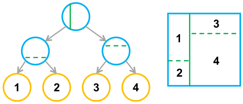
Figure 6: Visualization of a $k$-d tree (left) and a region it partitions (right). The parameters of each inner node (blue) are a fixed dimension, indicated by the orientation of the line used for partitioning, and a predicted threshold, indicated by the position of the line along the fixed dimension.

While BSPSegNet and SegForestNet only use BSP trees, differentiable rendering of other tree structures is possible by using the same region map R approach. A $k$-d tree [1], as shown in Fig. 6, is spatial partitioning data structure similar to a BSP tree that be used to partition a space with an arbitrary number of dimensions. It is also a binary tree. Instead of using a signed distance function to decide on which side of a boundary a given point lies, each inner node of $k$-d tree uses a threshold and a dimension index to decide whether a point lies in the left or right subset. The threshold $t$ is a value that needs to predicted while the dimension index $i$ is a fixed value chosen when instantiating the model. Eqs. 5-7 can be used for $k$-d trees as well with the signed distance function

$$f_{7}(\textbf{p})=t-\textbf{p}_{i}$$ (24)

where $\textbf{p}_{i}$ is the $i$-th component of the vector p. An inner node of a $k$-d tree requires only a single parameter to be predicted as opposed to the three to five parameters required for the signed distance functions used by an inner node of a BSP tree. However, generally $k$-d trees need to be deeper, e.g., to be able to define slopes, which counteracts this advantage. This depth disadvantage can be mitigated by making $i$ a predicted parameter. We call a tree with such inner nodes a dynamic $k$-d tree. A downside of this mitigation strategy is that one or two additional parameters (depending on the implementation) need to be predicted per inner node to decide whether the first dimension $i=1$ or the second dimension $i=2$ shall be used for partitioning. Even with this extra flexibility a dynamic $k$-d tree still has a depth disadvantage in the worst case, e.g., in the aforementioned slope example.

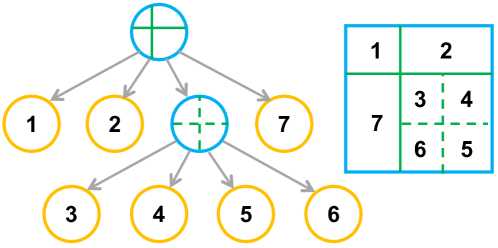
Figure 7: Visualization of a quadtree (left) and a region it partitions (right). The parameters of each inner node (blue) are the predicted coordinates of a point. This point partitions a given region into four quadrants which are then children of the associated inner node.

A quadtree [9], shown in Fig. 7, is a spatial partitioning data structure specifically designed to partition two dimensional planes. In each inner node of a quadtree a point x is used to partition the space into four quadrants. Compared to a $k$-d tree, a quadtree inner node partitions a space along both dimensions instead of only a single fixed dimension $i$ and it uses a different threshold $t$ for each dimension by using the components of x as thresholds. The equations

$$t_{1}=\textbf{x}_{1}-\textbf{p}_{1},t_{2}=\textbf{x}_{2}-\textbf{p}_{2}$$ (25)

$$t_{3}=\text{ReLU}(t_{1}),t_{4}=\text{ReLU}(-t_{1})$$ (26)

$$t_{5}=\text{ReLU}(t_{2}),t_{6}=\text{ReLU}(-t_{2})$$ (27)

$$\textbf{R}_{iyx}:=\textbf{R}_{iyx}+\lambda\cdot t_{4}\cdot t_{5}$$ (28)

$$\textbf{R}_{iyx}:=\textbf{R}_{iyx}+\lambda\cdot t_{3}\cdot t_{5}$$ (29)

$$\textbf{R}_{iyx}:=\textbf{R}_{iyx}+\lambda\cdot t_{4}\cdot t_{6}$$ (30)

$$\textbf{R}_{iyx}:=\textbf{R}_{iyx}+\lambda\cdot t_{3}\cdot t_{6}$$ (31)

are used to update the region map R for a quadtree at a location $\textbf{p}=(x,y)$. Note: in Eqs. 28-31 $i$ refers to indices of leaf nodes reachable from one of the child nodes. In Eq. 28 $i$ needs to be set to the indices of the leaf nodes covering the top-left partition, in Eq. 29 $i$ refers to the top-right partition, in Eq. 30 $i$ refers to the bottom-left partition and in Eq. 31 $i$ refers to the bottom-right partition.

This region map R based framework is general enough to even allow for trees in which different inner nodes are instances of different tree types (BSP, $k$-d, quadtree) or use different signed distance functions in the case of BSP tree inner nodes. When using class-specific trees, i.e., when partitioning the set of classes $C$ into subsets $C_{j}$, separate region maps specific to each of the subsets have to be computed anyway. Consequently, different tree configurations can be used for each of the subsets $C_{j}$ if so desired.

4 Evaluation

In this section we evaluate our contributions. First, we describe the datasets and the test setup we used. We will then present a toy example which proves that our generalizations in section 3.6 may be helpful if the alternate signed distance functions or tree structures suit the data. We then explore good value ranges for the hyperparameters we introduced, followed by an ablation study. We finish the section with a comparison to state-of-the-art models.

4.1 Datasets

We used seven different datasets for evaluation. We used aerial images, in particular true orthophotos, from the German cities Hannover, Buxtehude, Nienburg, Vaihingen and Potsdam. The later two datasets are part of the ISPRS 2D Semantic Labeling Benchmark Challenge [18]. Additionally, we used images from Toulouse [33]. The Toulouse dataset also includes instance labels for buildings for performing panoptic segmentation or instance segmentation. However, we only used the semantic labels. Our last dataset was iSAID [42], which is actually an instance segmentation dataset based on the object detection dataset DOTA [44]. Again, we ignored the instance labels. However due to its origin, iSAID has very sparse non-background labels, i.e., it cannot be considered a true semantic segmentation datasets which have much denser non-background label coverage.

Hannover, Buxtehude and Nienburg consist of 16 patches of $2500\times 2500$ pixels each. We omitted one such patch from Hannover since it consisted almost entirely of trees. We randomly divided the image patches into subsets s.t. roughly $70\%$ of pixels were used for training with the remainder split evenly into validation and test sets. Since Toulouse consists of only four images, we used two for training, one for validation and one for testing. iSAID is already pre-split into training and validation. We used the validation images as our test images and split the training set into training ($95\%$ of pixels) and actual validation. For Vaihingen and Potsdam, we used the images originally released without ground truth as test images and used the remaining images as training (roughly $90\%$ of pixels) and validation (roughly $10\%$ of pixels).

The ground truth classes of the German city images are impervious surfaces, buildings, low vegetation, tree, car, and clutter/background, the later two being rare. The Toulouse dataset also contains sports venues and water as separate classes in addition to the classes used for segmentation of the German cities. In Toulouse the classes car, sports venues, water, and background are rare. Since the background class is so rare and also is used to express uncertainty about the true class in the case of at least Potsdam, we ignored this class for all metrics, including training losses. The exception is the iSAID. Due to its sparsity of non-background pixels, less than $3\%$ of pixels belong to a non-background class, we did not ignore the background class in this case. iSAID has 15 non-background classes including different vehicle and sports venue categories.

For data augmentation, we randomly sampled 8000 input patches from the training images. The position (random translation) of the input patches was chosen s.t. input patches from the entire image could be sampled. The size of the square area being sampled was randomly scaled between $70\%$ and $130\%$ of $224\times 224$ pixels, the actual input size, making objects randomly appear smaller or larger for augmentation. The same scaling was applied to both spatial dimensions. The random shearing was chosen independently for both axes, sampled uniformly from $[-6\degree,6\degree]$. Random rotation depended on the dataset and was chosen from $[-50\degree,50\degree]$ for Vaihingen and from $[-30\degree,30\degree]$ for all other datasets. This dataset-specific augmentation for Vaihingen improved results on this dataset slightly. No flipping (horizontal or vertical) was used. All channels were normalized to zero mean and a standard deviation of $1$. After normalization, noise sampled from a normal distribution with standard deviation $0.1$ was added. The noise was sampled for each pixel and each channel individually. Furthermore, we used bilinear filtering. For the ground truth, we used the bilinear interpolation coefficients as voting weights to determine the discrete class for each pixel. Validation and test images were partitioned into axis-aligned input patches with no overlap and stride equal to the input patch size. We performed this input patch creation once for each dataset. Additionally, we computed the NDVI [34] for all datasets but iSAID, which lacks the necessary infrared channel. Other exceptions made for iSAID were sampling 28000 input patches and ensuring that the entropy of the class distribution of each sample was at least $0.04$ to ensure that the patches actually contained non-background pixels.

We used all available input channels and therefore adapted the number of input channels of the very first convolution of every model to the dataset used. All datasets except Vaihingen, which has no green channel, consist of at least RGB images with a few grayscale images in iSAID which we converted to RGB. The German cities all also have infrared channels and a digital surface model (”depth”). Toulouse actually consists of multispectral images with eight channels, including RGB and infrared.

4.2 Training and Test Setup

We used PyTorch v1.10 with CUDA 10.2 to train models on nVidia GeForce RTX 2080 Ti GPUs. Depending on the backbone used, we set the mini-batch size to 36 (MobileNetv2 [35]) or 18 (all other backbones). As an optimizer we used AdamW [20, 27] with a cosine annealing learning rate schedule [26]. As loss function we either used categorical cross entropy or our novel loss function (Eq. 14). For the cross entropy part, we set class weights s.t. rarer classes have higher weights based on the class distribution in the training images.

We used random search for hyperparameter optimization for all models, in particular optimizing their learning rates. For this, we computed the mean Intersection-over-Union (mIoU) on the validation subset of Buxtehude. We then used the maximum validation mIoU across all epochs of a run with a randomly chosen value for the hyperparameter being optimized to evaluate the performance of this run and thus hyperparameter value. The final hyperparameters used can be found in our published code. After hyperparameter optimization, we ran each experiment ten times and computed means and standard deviations from these ten runs. For the final comparison of our contributions to the state-of-the-art, we again used the maximum validation mIoU to identify the epoch after which each model performed best and then evaluated these particular model parameters on the test data.

We also made some small modifications to state-of-the-art models and backbones to either improve their performance slightly or simplify them while keeping their performance the same: we use LeakyReLUs [46] instead of ReLUs and we removed all atrous/dilated convolutions. For DeepLabv3+ we modified the strides of the backbone s.t. the spatial bottleneck had a downsampling factor of $8$. Training all models from scratch, we changed the first convolution in each backbone to accept all input channels offered by each respective dataset.

For the decoder of SegForestNet we used eight residual blocks with $F_{intermediate}=96$ (see Fig. 4). For the shape features, $F_{encoder}$ and $F_{tree}$ were set to $8$ and $9$ respectively. For the content features, we chose $F_{encoder}=16$ and $F_{tree}=4\cdot|C|$ with $|C|$ being the number of classes in the dataset. The numbers for $F_{tree}$ are the result of using BSP trees with depth $=2$, i.e., trees with three inner nodes and four leaf nodes.

4.3 Toy Experiment

While the generalization to different signed distance functions and different tree structures does not provide benefits for the semantic segmentation of aerial images, we still performed two experiments using toy datasets to show that these generalization may prove useful in other contexts. In street scenes captured by cameras attached to cars or in industrial applications rounded shapes, e.g., tires, pipes or drums, may occur frequently and thus a signed distance function capturing such shapes more accurately, e.g. $f_{3}$ (Eq. 20), may prove beneficial.

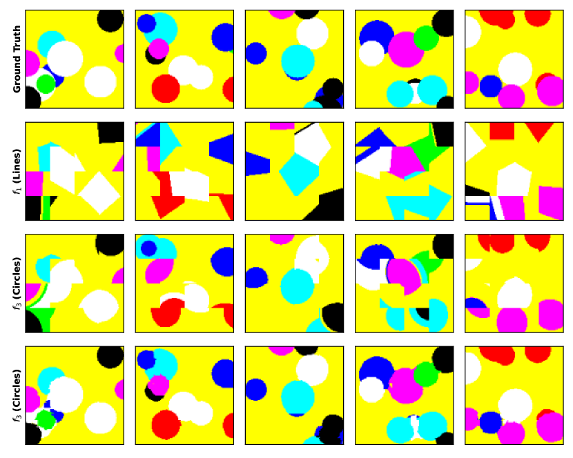
Figure 8: Toy dataset showing randomly created circles on a solid background. The ground truth visualization is equal to the input images, as there was a one-to-one correspondence of colors to classes. Using a signed distance function more suitable to the data (third row) produces more accurate predictions compared to using the default line-based signed distance function (second row). The restricted models in rows two and three were chosen to make the difference more visually obvious. The last row shows the prediction of a less restricted model to prove that the alternate signed distance functions can produce good results.

We created the first toy dataset by generating $128\times 128$ pixel RGB images showing circles as depicted in Fig. 8. We only used the eight corners of the RGB cube as colors and assigned a different class to each corner/color. One color was used as background and circles of random translation, size and color were drawn onto the background. The background color was never used for any of the random circles. We used a model which subdivides the image into blocks of size $32\times 32$ instead of $8\times 8$. For each block a shallow BSP tree of depth one was predicted. We heavily limited the prediction capability of the model to make the visual difference more clear. We trained the model ten times using $f_{1}$ (Eq. 18) in the inner nodes and ten times using $f_{3}$ (Eq. 20) instead. Using $f_{1}$, the model achieves an average validation mIoU of $63.3\%$ ($\pm 0.9\%$) across the ten trainings, while the $f_{3}$-based model achieves $64.9\%$ ($\pm 1.9\%$). The model with the more data-appropriate signed distance function, $f_{3}$, performed better.

While a tree depth of one, i.e., only a single inner node in each tree, might suggest that every $32\times 32$ block may contain only two different classes, there are blocks with three or more classes. An example is visible in the bottom-left of the $f_{1}$-based prediction in the last column of Fig. 8. This is due to the linear combination of the class logit predictions in the leaf nodes. To understand this phenomenon, suppose the predicted class logits are represented by the vectors $(v_{1},v_{2},0)$ and $(0,v_{2},v_{3})$ with $v_{1}>v_{2}>0$ and $v_{3}>v_{2}>0$ with the five missing dimensions for the other classes all being $0$ in both vectors. For any pixel in the segmentation the region map consists of a vector of the form $(\alpha,1-\alpha)$, i.e., the predicted class logits are $\alpha\cdot(v_{1},v_{2},0)+(1-\alpha)\cdot(0,v_{2},v_{3})=(\alpha v_{1},v_{2},(1-\alpha)v_{3})$. Depending on the value of $\alpha\in(0,1)$, which itself is dependent on the signed distance of the pixel to the decision boundary, the largest class logit may be $\alpha v_{1}$, $v_{2}$, or $(1-\alpha)v_{3}$, thus resulting in three regions with different classes despite there being only a single decision boundary. With other class logit distributions even more distinct regions are possible.

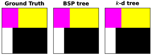
Figure 9: Toy dataset for investigating the impact of different tree structures. Again, the ground truth visualization is equal to the input images. Both tested tree structures can segment the images in the dataset perfectly eventually if the model is trained sufficiently long.

The toy dataset for the second experiment was created by partitioning $128\times 128$ pixel RGB vertically into two segments and then partitioning each segment horizontally resulting in examples as shown in Fig. 9. As before, we used the corners of the RGB cube as colors and classes. The resulting images can be perfectly segmented by a BSP tree of depth two using $f_{1}$ as signed distance function as well as by a $k$-d tree of depth two. However, the $k$-d tree needs fewer parameters to describe the inner nodes, thus is more efficient. For both tree structures, BSP trees and $k$-d trees, we trained ten models using this toy dataset. Both models eventually learned to segment the toy images perfectly, with the $k$-d trees having the negligible advantage of reaching this state an epoch or two sooner. The experiment still proves that region map-based differentiable rendering generalizes to other tree structures which may be desirable for types of data other than aerial images.

4.4 New Hyperparameters

We introduced several new hyperparameters throughout our contributions, $\lambda$ in Eq. 5 and $\mu_{1}$ to $\mu_{4}$ in Eq. 14. To study them, we used SegForestNet with MobileNetv2 as backbone, BSP trees using $f_{1}$ (Eq. 18) as signed distance function and a tree depth of 2. As we expect $\lambda$ to have no real effect anyway, especially since we introduced $\mu_{4}$, we simply set $\lambda=1$ and did not study it further. We ran random searches with 100 to 200 iterations to optimize each of the different $\mu_{i}$. We optimized $\mu_{3}$ and $\mu_{4}$ together in the same random search. We set $s_{\text{min}}=8$ (Eq. 12), i.e., each of the four regions should use at least one eighth of the area of each block. We chose this as a compromise, so that each region in a $8\times 8$ block contributes a significant part without restricting the model too much by setting $s_{\text{min}}$ too high.

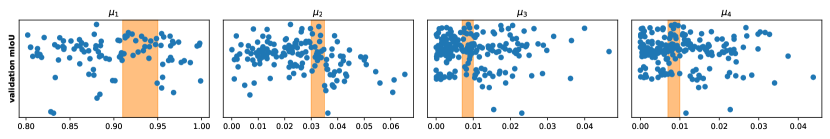
Figure 10: Validation mIoU on Buxtehude across $\mu_{i}$ (Eq. 14). As all $\mu_{i}$ except $\mu_{3}$ and $\mu_{4}$ were optimized in separate random searches, the corresponding mIoU ranges differ. However, as only finding the proper settings for $\mu_{i}$ is important, the exact mIoU ranges do not matter anyway. The highlighted intervals show the optimal range for each $\mu_{i}$.

The results of our random searches are shown in Fig. 10. The impact of cross-entropy, which was controlled by $\mu_{1}$, was the most significant. It also had a rather large range of $0.91$ to $0.95$ in which it produced optimal results. The other $\mu_{i}$ produced a slight increase in performance as they were increased, especially when considering the lower bound of the performance, with rather sharp drops in performance beyond a certain threshold. For $\mu_{2}$ that threshold was $0.035$, while it was $0.01$ for $\mu_{3}$ and $\mu_{4}$. We therefore chose values for $\mu_{2}$ to $\mu_{4}$ which were just below that threshold: $\mu_{2}=0.034$ and $\mu_{3}=\mu_{4}=0.0095$. We then computed $\mu_{1}=1-(\mu_{2}+\mu_{3}+\mu_{4})=0.947$ which is still in the optimal range for $\mu_{1}$. We therefore picked these values for the hyperparameters in Eq. 14.

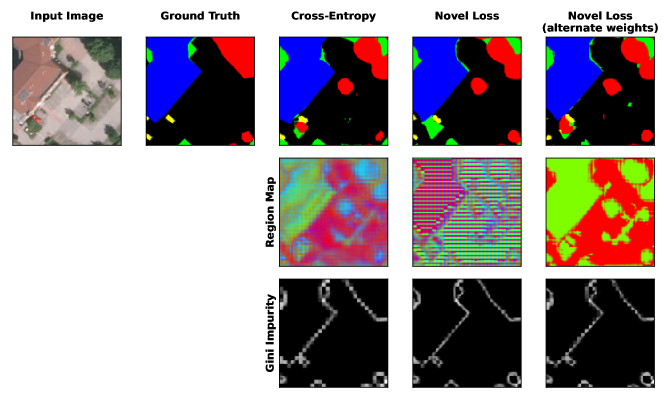
Figure 11: Visualization of the region map R and the Gini impurity $H$ (Eq. 11) for different loss functions and different values for $\mu_{i}$ (Eq. 14). The second to last column used optimized values for $\mu_{i}$, while the last column used $\mu_{1}=0.95$, $\mu_{2}=\mu_{3}=0$, and $\mu_{4}=0.05$. These visualizations show that our novel loss achieves the desired effects of sharp region boundaries and minimum region sizes (middle row) and pure regions containing just a single class according to the ground truth (bottom row).

In order to verify that the different loss components have the desired effects, we created a visualization of the region map R and the Gini impurity $H$ (Eq. 11). To create these visualizations, we used a variant of Eq. 4 in which we used colors or $H(\textbf{P}_{\textbf{B}}^{i})$ in place of the class logits $\textbf{v}_{i}$. Using colors (red, green, blue, and cyan) instead of class logits created a visualization showing which pixel belongs to which of the four regions in a block (Fig. 11, middle row). Using $H(\textbf{P}_{\textbf{B}}^{i})$ instead created a visualization highlighting pixels in gray or even white which belong to regions which contain more than one class according to the ground truth (Fig. 11, bottom row). Using our novel loss with optimized values for $\mu_{i}$ created region maps with the desired minimum region size and sharp region boundaries. Furthermore, the average $H(\textbf{P}_{\textbf{B}}^{i})$ are smaller compared to using cross-entropy. Cross-entropy also created blurry boundaries and seemed to associate certain regions with certain classes: the green region was used for buildings (blue in the ground truth), the cyan region was used for trees (red in the ground truth) and the red region for the remaining classes. Using our novel loss but with unoptimized $\mu_{i}$, in particular setting $\mu_{2}$ (pure regions containing only class according to the ground truth) and $\mu_{3}$ (minimum region size) to $0$, showed that the individual losses have the desired effects. The average $H(\textbf{P}_{\textbf{B}}^{i})$ is slightly higher (hard to see in Fig. 11) and certain regions (blue and cyan) are never used. Still, the region boundaries are sharp since $\mu_{4}$ is sufficiently high.

4.5 Ablation Study

In an ablation study, shown in Table I, we examined the effect of each contribution individually. As before, we used SegForestNet with MobileNetv2 as backbone. The new region map computation (Eqs. 5 to 7) had the greatest impact. Not only did it improve performance and reduce the variance, it was also required for the novel loss to actually provide a benefit. Without the new region map computation the new decoder architecture also provided a significant performance improvement but without the reduction in variance. With the new region map computation there was still a small performance improvement provided by the new decoder architecture. Furthermore, the new decoder architecture reduced the total model size by $5\%$ due to each decoder using only $85.3$k parameters instead of $137.7$k. As mentioned before, the novel loss only was beneficial in combination with the new region map computation and even then the improvements were rather small. Overall, there was an improvement of almost $1\%$ when using all contributions. We did not include class-specific trees in this ablation study as their benefit is dataset dependant which we show in the next section.

TABLE I: Ablation study. The top-most row is SegForestNet with all our contributions, while the bottom-most row is the original BSPSegNet. The last column shows max. validation mIoU on Buxtehude.

new	new region	novel
decoder	map computation	loss	mIoU
✓	✓	✓	$77.4\%\pm 0.2\%$
✓	✓		$77.3\%\pm 0.1\%$
✓		✓	$76.8\%\pm 1.5\%$
✓			$77.3\%\pm 0.3\%$
	✓	✓	$77.3\%\pm 0.2\%$
	✓		$77.1\%\pm 0.2\%$
		✓	$73.1\%\pm 1.9\%$
			$76.5\%\pm 1.5\%$

4.6 Comparison to State-Of-The-Art

Finally, we compared SegForestNet to state-of-the-art models. Results are shown in Table II and Fig. 12 with samples of predicted segmentations in Fig. 13. We grouped models according to their number of parameters (Table III) in order to be able to compare models of similar size and complexity with each other. We created four groups, small models (less than five million parameters), medium size models (around ten million parameters), large models (20 to 30 million parameters) and very large models (more than 30 million parameters). Since all tested models except U-Net and U-Net++ have interchangeable backbones we tested all models in a smaller variant, using MobileNetv2 as a backbone, and a larger variant, using Xception as a backbone. With these two backbones, SegForestNet appears in the small model and the large model group. Additionally, SegForestNet was tested in two variants, the base variant in which only a single BSP tree per $8\times 8$ block was predicted, and a variant, SegForestNet*, in which one BSP tree per class per block was predicted. Some older models, e.g., U-Net, still show competitive performance and thus we chose a selection of older and newer models to compare SegForestNet to: FCN [25], DeepLab v3+ [4], (S-)RA-FCN [29], PFNet [24], FarSeg [50], U-Net++ [51] and U-Net [32].

TABLE II: Average test mIoU across ten runs for various models. Our models are SegForestNet and SegForestNet*. Models marked with ${\dagger}$ use Xception as the backbone, while all others use MobileNetv2 instead. The two U-Net variants are an exception, since they have a fixed architecture rather then exchangeable backbones. The models are grouped according to their size (Table III) with the best model in each bracket highlighted in bold.

	Hannover	Nienburg	Buxtehude	Potsdam	Vaihingen	Toulouse	iSAID
FCN	$72.6\%\pm 0.2\%$	$73.2\%\pm 0.4\%$	$76.2\%\pm 0.2\%$	$78.1\%\pm 0.2\%$	$72.0\%\pm 0.2\%$	$54.1\%\pm 2.9\%$	$38.3\%\pm 0.9\%$
SegForestNet	$72.9\%\pm 0.5\%$	$73.8\%\pm 0.3\%$	$76.2\%\pm 0.3\%$	$\textbf{78.9}\%\pm 0.3\%$	$72.9\%\pm 0.3\%$	$52.9\%\pm 3.2\%$	$44.5\%\pm 0.7\%$
DeepLab v3+	$72.9\%\pm 0.3\%$	$73.8\%\pm 0.3\%$	$76.5\%\pm 0.3\%$	$77.8\%\pm 0.8\%$	$72.2\%\pm 0.3\%$	$52.8\%\pm 3.8\%$	$34.9\%\pm 1.2\%$
RA-FCN	$71.0\%\pm 0.4\%$	$71.0\%\pm 0.4\%$	$74.1\%\pm 0.8\%$	$74.1\%\pm 1.1\%$	$70.3\%\pm 0.3\%$	$49.4\%\pm 2.2\%$	$35.4\%\pm 4.1\%$
SegForestNet*	$\textbf{73.6}\%\pm 0.2\%$	$74.1\%\pm 0.3\%$	$76.2\%\pm 0.2\%$	$78.8\%\pm 0.3\%$	$\textbf{72.9}\%\pm 0.2\%$	$\textbf{54.2}\%\pm 1.6\%$	$42.8\%\pm 0.5\%$
PFNet	$73.0\%\pm 0.4\%$	$\textbf{74.2}\%\pm 0.3\%$	$\textbf{76.8}\%\pm 0.4\%$	$\textbf{78.9}\%\pm 0.3\%$	$72.6\%\pm 0.2\%$	$53.9\%\pm 1.3\%$	$\textbf{45.8}\%\pm 0.4\%$
FarSeg	$72.9\%\pm 0.3\%$	$74.2\%\pm 0.2\%$	$76.7\%\pm 0.2\%$	$\textbf{77.6}\%\pm 0.5\%$	$\textbf{72.2}\%\pm 0.3\%$	$54.5\%\pm 1.9\%$	$43.4\%\pm 0.8\%$
U-Net++	$\textbf{73.8}\%\pm 0.3\%$	$\textbf{75.6}\%\pm 0.2\%$	$\textbf{77.4}\%\pm 0.2\%$	$77.3\%\pm 0.3\%$	$71.7\%\pm 0.2\%$	$\textbf{56.8}\%\pm 2.0\%$	$\textbf{45.4}\%\pm 0.6\%$
$\text{FCN}^{\dagger}$	$73.4\%\pm 0.1\%$	$74.1\%\pm 0.2\%$	$76.4\%\pm 0.2\%$	$79.4\%\pm 0.2\%$	$72.7\%\pm 0.2\%$	$54.3\%\pm 1.1\%$	$48.4\%\pm 0.5\%$
$\text{SegForestNet}^{\dagger}$	$73.7\%\pm 0.5\%$	$74.5\%\pm 0.3\%$	$76.8\%\pm 0.1\%$	$79.1\%\pm 0.3\%$	$73.1\%\pm 0.4\%$	$55.1\%\pm 0.7\%$	$50.4\%\pm 0.6\%$
$\text{DeepLab v3+}^{\dagger}$	$73.5\%\pm 0.2\%$	$74.7\%\pm 0.2\%$	$76.6\%\pm 0.2\%$	$78.8\%\pm 0.2\%$	$72.7\%\pm 0.3\%$	$55.2\%\pm 0.6\%$	$48.9\%\pm 0.3\%$
$\text{SegForestNet*}^{\dagger}$	$\textbf{74.0}\%\pm 0.3\%$	$74.3\%\pm 0.5\%$	$76.9\%\pm 0.2\%$	$79.5\%\pm 0.2\%$	$72.9\%\pm 0.3\%$	$53.8\%\pm 1.3\%$	$49.2\%\pm 0.8\%$
$\text{PFNet}^{\dagger}$	$73.9\%\pm 0.2\%$	$\textbf{74.9}\%\pm 0.2\%$	$\textbf{77.2}\%\pm 0.2\%$	$\textbf{79.6}\%\pm 0.4\%$	$\textbf{73.3}\%\pm 0.3\%$	$\textbf{55.2}\%\pm 1.6\%$	$\textbf{50.6}\%\pm 0.2\%$
$\text{FarSeg}^{\dagger}$	$54.3\%\pm 29.6\%$	$61.7\%\pm 25.9\%$	$56.3\%\pm 29.6\%$	$64.3\%\pm 27.6\%$	$59.5\%\pm 25.9\%$	$54.8\%\pm 1.8\%$	$46.3\%\pm 3.2\%$
U-Net	$\textbf{74.4}\%\pm 0.1\%$	$\textbf{75.8}\%\pm 0.2\%$	$\textbf{77.2}\%\pm 0.5\%$	$\textbf{78.2}\%\pm 0.5\%$	$\textbf{71.5}\%\pm 0.3\%$	$\textbf{57.3}\%\pm 0.9\%$	$\textbf{47.8}\%\pm 0.3\%$
$\text{RA-FCN}^{\dagger}$	$67.0\%\pm 1.5\%$	$69.1\%\pm 0.3\%$	$71.4\%\pm 0.8\%$	$72.6\%\pm 0.8\%$	$65.5\%\pm 1.5\%$	$48.2\%\pm 1.9\%$	$34.0\%\pm 1.4\%$

TABLE III: Size of the tested models in terms of number of model parameters as a proxy for model complexity. We grouped the models in four brackets: small (less than 5M), medium (about 10M), large (20-30M), and very large (more than 30M). The symbol ${\dagger}$ is used as in Table II.

	# of model parameters [M]
FCN	1.8
SegForestNet	2.0
DeepLab v3+	2.3
RA-FCN	2.3
SegForestNet*	2.9 - 4.7
PFNet	4.9
FarSeg	9.1
U-Net++	9.2
$\text{FCN}^{\dagger}$	20.9
$\text{SegForestNet}^{\dagger}$	21.1
$\text{DeepLab v3+}^{\dagger}$	22.2
$\text{SegForestNet*}^{\dagger}$	22.2 - 24.4
$\text{PFNet}^{\dagger}$	26.4
$\text{FarSeg}^{\dagger}$	29.2
U-Net	31.4
$\text{RA-FCN}^{\dagger}$	40.0

TABLE IV: Count of how often each model appears in the Pareto front of a given dataset (compare Fig. 12). SegForestNet’ is a combination of SegForestNet or SegForestNet*: if either of the later two is in the Pareto front of a given dataset, the count for SegForestNet’ is increased by 1. The symbol ${\dagger}$ is used as in Table II.

# of times in
Pareto front	models
7	FCN
6	SegForestNet’
5	SegForestNet
4	SegForestNet*, U-Net++, $\text{SegForestNet'}^{\dagger}$
3	PFNet, $\text{PFNet}^{\dagger}$, U-Net
2	$\text{FCN}^{\dagger}$, $\text{SegForestNet}^{\dagger}$, $\text{SegForestNet*}^{\dagger}$
1	DeepLab v3+, FarSeg
0	RA-FCN, $\text{DeepLab v3+}^{\dagger}$, $\text{FarSeg}^{\dagger}$, $\text{RA-FCN}^{\dagger}$

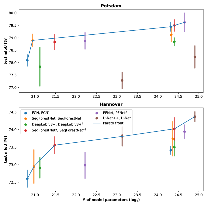
Figure 12: Visualization of the columns for Potsdam and Hannover from Table II. Dots show means and bars indicate the standard deviation. The symbol ${\dagger}$ is used as in Table II.

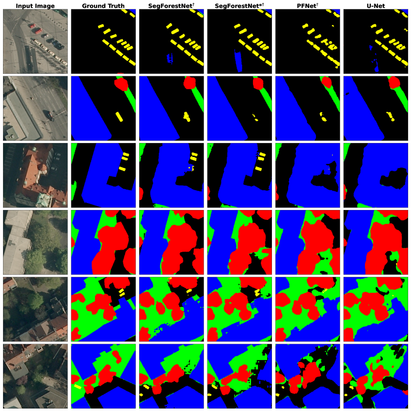
Figure 13: Samples of validation and test examples from Hannover. All models except U-Net use Xception as backbone.

We trained all models ourselves: we used optimized parameters suggested by the respective authors, except that we optimized the learning rates via random search. All models were trained ten times. To avoid overfitting, we used the validation mIoU for each training run to identify the epoch in which the model performed best and then used the parameters from this best epoch to determine the mIoU on the test set. All results shown are the average test mIoUs.

There is no clear winner between SegForestNet and its variant SegForestNet*. Sometimes, e.g, when using the MobileNetv2 backbone to train a model on Potsdam or iSAID, SegForestNet performs better while at other times, e.g., same backbone but training on Hannover or Toulouse, SegForestNet* performs better. The situation may even differ for different backbones on the same dataset, e.g., when using the Xception backbone to train a model on Potsdam, SegForestNet* outperforms SegForestNet. Therefore, no clear recommendation whether to use class-specific segmentations (SegForestNet*) or not (SegForestNet) can be given. Rather, this is has to be determined based on the backbone and dataset to be used.

On all datasets except iSAID most models performed well, even older models. The exceptions were RA-FCN and FarSeg. RA-FCN throughout performed noticably worse than all other models. It also has scaling issues, as its number of parameters increased far more when going from the MobileNetv2 backbone to the Xception backbone while at the same time its performance became worse instead of better. FarSeg’s performance with MobileNetv2 was decent (when ignoring the full model’s relatively large size) but its performance became very unstable when using Xception. Due to these noticable performance deficits, we excluded RA-FCN and FarSeg in Fig. 12.

Generally, the best peforming models appeared to be SegForestNet (in at least one variant), PFNet, U-Net++ and U-Net. In the small and large model brackets the best performing model always is SegForestNet, SegForestNet* or PFNet. Most of the time at least one SegForestNet variant and PFNet are very close in performance. In the small model bracket, SegForestNet is the best model once, while SegForestNet* is so three times and PFNet is the best model four times (SegForestNet and PFNet share their victory on Potsdam). In the large model segment, SegForestNet* is the best model once and PFNet is the best model on all other datasets. But again, when compared to the standard deviation, the SegForestNet variants and PFNet can be said to perform equally well most of the time. In the other model size brackets, U-Net++ and U-Net almost always performed best, however, there was little competition in these brackets.

An advantage SegForestNet has over the competition is that the model is relatively small. When using MobileNetv2 for all models and comparing to PFNet, it uses almost $60\%$ fewer parameters. SegForestNet* uses up to $40\%$ fewer parameters than PFNet, depending on the dataset since the number of predicted trees depends on the numer of classes in the dataset. These numbers decrease to $20\%$ and $16\%$ respectively when moving from MobileNetv2 to Xception as a backbone. SegForestNet’s advantage is even larger when compared to the U-Net variants. This, same performance at a much smaller size, proves that the prediction of polygons instead of allowing arbitrary shapes, is a useful inductive bias to learning the semantic segmentation of aerial and satellite images. With dataset size and therefore overfitting being a common problem for aerial image analysis, smaller models are beneficial as they are less prone to overfitting.

What the best model for a given dataset is also depends on the computational budget available. We used the number of model parameters as a proxy for this budget and computed how often each model appeared in the Pareto front, see Fig. 12, in each of the seven datasets. The results are shown in Table IV. The table again highlights that the SegForestNet variants, PFNet and the U-Net variants are the top models. The seemingly good performance of FCN with MobileNetv2 is simply due to it being the smallest model in the comparison. Which model is the best suited depends on the dataset and the available computational budget.

Fig. 13 shows a qualitative comparison of the best models. All of these models provide good results, while no model is perfect. SegForestNet generally performs better for cars. The other models more often overlook cars entirely and tend to have multiple distinct car segments merge into each other. Areas in shadow proof difficult for all shown models with sealed surfaces sometimes mistaken as buildings or low vegetation/grass mistaken as sealed surface. SegForestNet tends to have straighter lines where appropriate, e.g., buildings and cars, while still being able to predict sufficiently rounded shapes, e.g., trees. However, when errors occur, e.g., when low vegetation in shadow gets mistaken as a sealed surface, SegForestNet produces visible block artefacts.

5 Conclusion

In this paper we present a model for the semantic segmentation of aerial images using binary space partitioning trees, as well as three modifications to this model to improve its performance. The first modificatios, a refined decoder and new region map computation strategy, are aimed at improving gradients during backpropagation, while the second is a novel loss function improving the shape of the predicted segments and the last modification is an extension which enables class-specific segmentations. Taking all modifications together, our model achieves state-of-the-art performance while using up to $60\%$ fewer model parameters when using a small backbone model or up to $20\%$ fewer model parameters when using a large backbone model. In the future, we want to investigate how to let our model learn by itself what the optimal type of tree, signed distance function in each inner node, and number of trees is for a given dataset. This would reduce the number of design decisions having to be made when applying our model. Additionally, we want to expand our model to be able to predict instance IDs in order to perform instance and/or panoptic segmentation.

References

- [1] Jon Louis Bentley. Multidimensional binary search trees used for associative searching. Communications of the ACM, 18(9):509–517, 1975.
- [2] Liang-Chieh Chen, George Papandreou, Iasonas Kokkinos, Kevin Murphy, and Alan L Yuille. Deeplab: Semantic image segmentation with deep convolutional nets, atrous convolution, and fully connected crfs. IEEE transactions on pattern analysis and machine intelligence, 40(4):834–848, 2017.
- [3] Liang-Chieh Chen, George Papandreou, Florian Schroff, and Hartwig Adam. Rethinking atrous convolution for semantic image segmentation. arXiv preprint arXiv:1706.05587, 2017.
- [4] Liang-Chieh Chen, Yukun Zhu, George Papandreou, Florian Schroff, and Hartwig Adam. Encoder-decoder with atrous separable convolution for semantic image segmentation. In ECCV, pages 801–818, 2018.
- [5] Zhiqin Chen, Andrea Tagliasacchi, and Hao Zhang. Bsp-net: Generating compact meshes via binary space partitioning. In Proceedings of the IEEE/CVF Conference on Computer Vision and Pattern Recognition, pages 45–54, 2020.
- [6] François Chollet. Xception: Deep learning with depthwise separable convolutions. In Proceedings of the IEEE conference on computer vision and pattern recognition, pages 1251–1258, 2017.
- [7] Özgün Çiçek, Ahmed Abdulkadir, Soeren S Lienkamp, Thomas Brox, and Olaf Ronneberger. 3d u-net: learning dense volumetric segmentation from sparse annotation. In International conference on medical image computing and computer-assisted intervention, pages 424–432. Springer, 2016.
- [8] Christer Ericson. Real-time collision detection. Crc Press, 2004.
- [9] Raphael A Finkel and Jon Louis Bentley. Quad trees a data structure for retrieval on composite keys. Acta informatica, 4(1):1–9, 1974.
- [10] Henry Fuchs, Zvi M Kedem, and Bruce F Naylor. On visible surface generation by a priori tree structures. In Proceedings of the 7th annual conference on Computer graphics and interactive techniques, pages 124–133, 1980.
- [11] Nicolas Girard, Guillaume Charpiat, and Yuliya Tarabalka. Aligning and updating cadaster maps with aerial images by multi-task, multi-resolution deep learning. In Asian Conference on Computer Vision, pages 675–690. Springer, 2018.
- [12] Georgia Gkioxari, Jitendra Malik, and Justin Johnson. Mesh r-cnn. In Proceedings of the IEEE/CVF International Conference on Computer Vision, pages 9785–9795, 2019.
- [13] Jairo A Gómez, Jorge E Patiño, Juan C Duque, and Santiago Passos. Spatiotemporal modeling of urban growth using machine learning. Remote Sensing, 12(1):109, 2020.
- [14] Daniel Gritzner and Jörn Ostermann. Semantic segmentation of aerial images using binary space partitioning. In German Conference on Artificial Intelligence (Künstliche Intelligenz), pages 116–134. Springer, 2021.
- [15] Kaiming He, Georgia Gkioxari, Piotr Dollár, and Ross Girshick. Mask r-cnn. In Proceedings of the IEEE international conference on computer vision, pages 2961–2969, 2017.
- [16] Kaiming He, Xiangyu Zhang, Shaoqing Ren, and Jian Sun. Deep residual learning for image recognition. In Proceedings of the IEEE conference on computer vision and pattern recognition, pages 770–778, 2016.
- [17] Sergey Ioffe and Christian Szegedy. Batch normalization: Accelerating deep network training by reducing internal covariate shift. In International conference on machine learning, pages 448–456. PMLR, 2015.
- [18] ISPRS. 2D Semantic Labeling - ISPRS. http://www2.isprs.org/commissions/comm3/wg4/semantic-labeling.html, 2020. Accessed: 2020-01-28.
- [19] Simon Jégou, Michal Drozdzal, David Vazquez, Adriana Romero, and Yoshua Bengio. The one hundred layers tiramisu: Fully convolutional densenets for semantic segmentation. In Proceedings of the IEEE conference on computer vision and pattern recognition workshops, pages 11–19, 2017.
- [20] Diederik P Kingma and Jimmy Ba. Adam: A method for stochastic optimization. arXiv preprint arXiv:1412.6980, 2014.
- [21] Alexander Kirillov, Kaiming He, Ross Girshick, Carsten Rother, and Piotr Dollár. Panoptic segmentation. In Proceedings of the IEEE/CVF Conference on Computer Vision and Pattern Recognition, pages 9404–9413, 2019.
- [22] Alexander Kirillov, Yuxin Wu, Kaiming He, and Ross Girshick. Pointrend: Image segmentation as rendering. In Proceedings of the IEEE/CVF conference on computer vision and pattern recognition, pages 9799–9808, 2020.
- [23] Seong-Hyeok Lee, Kuk-Jin Han, Kwon Lee, Kwang-Jae Lee, Kwan-Young Oh, and Moung-Jin Lee. Classification of landscape affected by deforestation using high-resolution remote sensing data and deep-learning techniques. Remote Sensing, 12(20):3372, 2020.
- [24] Xiangtai Li, Hao He, Xia Li, Duo Li, Guangliang Cheng, Jianping Shi, Lubin Weng, Yunhai Tong, and Zhouchen Lin. Pointflow: Flowing semantics through points for aerial image segmentation. In Proceedings of the IEEE/CVF Conference on Computer Vision and Pattern Recognition, pages 4217–4226, 2021.
- [25] Jonathan Long, Evan Shelhamer, and Trevor Darrell. Fully convolutional networks for semantic segmentation. In CVPR, pages 3431–3440, 2015.
- [26] Ilya Loshchilov and Frank Hutter. Sgdr: Stochastic gradient descent with warm restarts. arXiv preprint arXiv:1608.03983, 2016.
- [27] Ilya Loshchilov and Frank Hutter. Decoupled weight decay regularization. arXiv preprint arXiv:1711.05101, 2017.
- [28] Lars Mescheder, Michael Oechsle, Michael Niemeyer, Sebastian Nowozin, and Andreas Geiger. Occupancy networks: Learning 3d reconstruction in function space. In Proceedings of the IEEE/CVF Conference on Computer Vision and Pattern Recognition, pages 4460–4470, 2019.
- [29] Lichao Mou, Yuansheng Hua, and Xiao Xiang Zhu. A relation-augmented fully convolutional network for semantic segmentation in aerial scenes. In Proceedings of the IEEE/CVF Conference on Computer Vision and Pattern Recognition, pages 12416–12425, 2019.
- [30] G Papandreou, L-Ch Chen, K Murphy, and AL Yuille. Weakly-and semi-supervised learning of a dcnn for semantic image segmentation. arxiv 2015. arXiv preprint arXiv:1502.02734.
- [31] Ulrike Pestel-Schiller, Ye Yang, and Jörn Ostermann. Semantic segmentation of natural and man-made fruits using a spatial-spectral two-channel-cnn for sparse data. In 12th Workshop on Hyperspectral Imaging and Signal Processing: Evolution in Remote Sensing (WHISPERS), September 2022.
- [32] Olaf Ronneberger, Philipp Fischer, and Thomas Brox. U-net: Convolutional networks for biomedical image segmentation. In International Conference on Medical image computing and computer-assisted intervention, pages 234–241. Springer, 2015.
- [33] Ribana Roscher, Michele Volpi, Clément Mallet, Lukas Drees, and Jan Dirk Wegner. Semcity toulouse: A benchmark for building instance segmentation in satellite images. ISPRS Annals of Photogrammetry, Remote Sensing and Spatial Information Sciences, V-5-2020:109–116, 2020.
- [34] John W Rouse Jr, R Hect Haas, JA Schell, and DW Deering. Monitoring the vernal advancement and retrogradation (green wave effect) of natural vegetation. Technical report, 1973.
- [35] Mark Sandler, Andrew Howard, Menglong Zhu, Andrey Zhmoginov, and Liang-Chieh Chen. Mobilenetv2: Inverted residuals and linear bottlenecks. In CVPR, pages 4510–4520, 2018.
- [36] Fabien Sanglard. Game Engine Black Book: DOOM v1.1. Sanglard, Fabien, 2019.
- [37] Karen Simonyan and Andrew Zisserman. Very deep convolutional networks for large-scale image recognition. arXiv preprint arXiv:1409.1556, 2014.
- [38] Konstantin Sofiiuk, Olga Barinova, and Anton Konushin. Adaptis: Adaptive instance selection network. In Proceedings of the IEEE/CVF International Conference on Computer Vision, pages 7355–7363, 2019.
- [39] Towaki Takikawa, David Acuna, Varun Jampani, and Sanja Fidler. Gated-scnn: Gated shape cnns for semantic segmentation. In Proceedings of the IEEE/CVF International Conference on Computer Vision, pages 5229–5238, 2019.
- [40] Maxim Tatarchenko, Alexey Dosovitskiy, and Thomas Brox. Octree generating networks: Efficient convolutional architectures for high-resolution 3d outputs. In Proceedings of the IEEE International Conference on Computer Vision, pages 2088–2096, 2017.
- [41] Nanyang Wang, Yinda Zhang, Zhuwen Li, Yanwei Fu, Wei Liu, and Yu-Gang Jiang. Pixel2mesh: Generating 3d mesh models from single rgb images. In Proceedings of the European Conference on Computer Vision (ECCV), pages 52–67, 2018.
- [42] Syed Waqas Zamir, Aditya Arora, Akshita Gupta, Salman Khan, Guolei Sun, Fahad Shahbaz Khan, Fan Zhu, Ling Shao, Gui-Song Xia, and Xiang Bai. isaid: A large-scale dataset for instance segmentation in aerial images. In Proceedings of the IEEE Conference on Computer Vision and Pattern Recognition Workshops, pages 28–37, 2019.
- [43] Huikai Wu, Junge Zhang, Kaiqi Huang, Kongming Liang, and Yizhou Yu. Fastfcn: Rethinking dilated convolution in the backbone for semantic segmentation. arXiv preprint arXiv:1903.11816, 2019.
- [44] Gui-Song Xia, Xiang Bai, Jian Ding, Zhen Zhu, Serge Belongie, Jiebo Luo, Mihai Datcu, Marcello Pelillo, and Liangpei Zhang. Dota: A large-scale dataset for object detection in aerial images. In The IEEE Conference on Computer Vision and Pattern Recognition (CVPR), June 2018.
- [45] Yuwen Xiong, Renjie Liao, Hengshuang Zhao, Rui Hu, Min Bai, Ersin Yumer, and Raquel Urtasun. Upsnet: A unified panoptic segmentation network. In Proceedings of the IEEE/CVF Conference on Computer Vision and Pattern Recognition, pages 8818–8826, 2019.
- [46] Bing Xu, Naiyan Wang, Tianqi Chen, and Mu Li. Empirical evaluation of rectified activations in convolutional network. arXiv preprint arXiv:1505.00853, 2015.
- [47] Tien-Ju Yang, Maxwell D Collins, Yukun Zhu, Jyh-Jing Hwang, Ting Liu, Xiao Zhang, Vivienne Sze, George Papandreou, and Liang-Chieh Chen. Deeperlab: Single-shot image parser. arXiv preprint arXiv:1902.05093, 2019.
- [48] Yibo Yang, Hongyang Li, Xia Li, Qijie Zhao, Jianlong Wu, and Zhouchen Lin. Sognet: Scene overlap graph network for panoptic segmentation. In Proceedings of the AAAI Conference on Artificial Intelligence, volume 34, pages 12637–12644, 2020.
- [49] Fisher Yu and Vladlen Koltun. Multi-scale context aggregation by dilated convolutions. arXiv preprint arXiv:1511.07122, 2015.
- [50] Zhuo Zheng, Yanfei Zhong, Junjue Wang, and Ailong Ma. Foreground-aware relation network for geospatial object segmentation in high spatial resolution remote sensing imagery. In Proceedings of the IEEE/CVF conference on computer vision and pattern recognition, pages 4096–4105, 2020.
- [51] Zongwei Zhou, Md Mahfuzur Rahman Siddiquee, Nima Tajbakhsh, and Jianming Liang. Unet++: A nested u-net architecture for medical image segmentation. In Deep learning in medical image analysis and multimodal learning for clinical decision support, pages 3–11. Springer, 2018.
- [52] Yi Zhu, Karan Sapra, Fitsum A Reda, Kevin J Shih, Shawn Newsam, Andrew Tao, and Bryan Catanzaro. Improving semantic segmentation via video propagation and label relaxation. In Proceedings of the IEEE/CVF Conference on Computer Vision and Pattern Recognition, pages 8856–8865, 2019.
Acknowledgments
The aerial images of the 3Cities dataset were provided by the Landesamt für Geoinformation und Landesvermessung Niedersachsen (LGLN; https://www.lgln.niedersachsen.de/startseite/) in 2013.