TT-TFHE: a Torus Fully Homomorphic Encryption-Friendly
Neural Network Architecture

Abstract

This paper presents TT-TFHE, a deep neural network Fully Homomorphic Encryption (FHE) framework that effectively scales Torus FHE (TFHE) usage to tabular and image datasets using a recent family of convolutional neural networks called Truth-Table Neural Networks (TTnet). The proposed framework provides an easy-to-implement, automated TTnet-based design toolbox with an underlying (python-based) open-source Concrete implementation (CPU-based and implementing lookup tables) for inference over encrypted data. Experimental evaluation shows that TT-TFHE greatly outperforms in terms of time and accuracy all Homomorphic Encryption (HE) set-ups on three tabular datasets, all other features being equal. On image datasets such as MNIST and CIFAR-10, we show that TT-TFHE consistently and largely outperforms other TFHE set-ups and is competitive against other HE variants such as BFV or CKKS (while maintaining the same level of 128-bit encryption security guarantees). In addition, our solutions present a very low memory footprint (down to dozens of MBs for MNIST), which is in sharp contrast with other HE set-ups that typically require tens to hundreds of GBs of memory per user (in addition to their communication overheads). This is the first work presenting a fully practical solution of private inference (i.e. a few seconds for inference time and a few dozens MBs of memory) on both tabular datasets and MNIST, that can easily scale to multiple threads and users on server side.

1 Introduction

Deep Neural Networks (DNNs) have achieved remarkable results in various fields, including image recognition, natural language processing or medical diagnostics. “Machine Learning as a Service” (MLaaS) is a recent and popular DNN-based business use-case (Philipp et al., 2020; Li et al., 2017; Ribeiro et al., 2015), where clients pay for predictions from a service provider. However, this approach requires trust between the client and the service provider. In cases where the data is sensitive, such as military, financial, or health information, clients may be hesitant (or are simply not allowed) to share their data with the service provider for privacy reasons. On the service provider’s side, training DNNs requires large amounts of data, technical expertise, and computer resources, which can be expensive and time-consuming. As a result, service providers may hesitate to give the model directly to the client, as it may be easily reverse-engineered (or at least make the attacker’s task much easier), hindering the growth of MLaaS activity. Allowing the clients to perform the inference locally is also not very practical as any model update would have to be pushed to all clients, not to mention the complex support of the various client hardware/software configurations, etc.

HE/FHE (Gentry, 2009) is an ideal technology to address Privacy-Preserving in Machine Learning (PPML) as it allows the computations to be performed directly on encrypted data. By encrypting its data before sharing it with the service provider, the client ensures that it remains private while the service provider can still provide accurate predictions. This solves the trust issue and also gives a competitive advantage in regions where data regulations are stricter, such as Europe’s General Data Protection Regulation (GDPR) (Regulation, 2016). The most popular HE schemes are BGV/BFV (Brakerski et al., 2014; Brakerski, 2012; Fan & Vercauteren, 2012), CKKS (Cheon et al., 2017) and Torus-FHE (TFHE) (Chillotti et al., 2016, 2020a) and this paper presents our proposed solution that utilizes TFHE to provide a privacy-preserving MLaaS framework for DNNs. TFHE enables very fast gate bootstrapping as well as circuit bootstapping and operations over Boolean gates. Moreover, extended versions of TFHE, such as Concrete (Chillotti et al., 2020b) allows programmable bootstrapping enabling evaluation of certain functions during the bootstrapping step itself.

The security and flexibility provided by HE come at a cost, as the computation, communication, and memory overheads are significant, especially for complex functions such as DNNs:

• Time overhead: on server side, an FHE logic gate computation within a TFHE scheme takes milliseconds  (Chillotti et al., 2016), compared to nanoseconds for a standard logic gate. On client side the overhead for encryption/decryption of the data is usually not an issue, as milliseconds are enough for those operations.

• Communication overhead: an MNIST image sent in clear represents a few kBs, while encrypted within any HE scheme it is of the order of a few MBs (excluding the public key which typically requires hundred(s) of MBs) (Clet et al., 2021). Moreover, PPML schemes not based on TFHE, such as those based on CKKS, require a significant communication overhead due to the need for multiple exchanges between the client and the cloud  (Clet et al., 2021).

• Memory overhead: TFHE-based schemes typically require a few of MBs of RAM on server side, while those based on CKKS need several GBs per image (Gilad-Bachrach et al., 2016; Brutzkus et al., 2019), even up to hundreds of GBs for the most time-efficient solutions (Lee et al., 2022) (384GB of RAM usage to infer a single CIFAR-10 image using ResNet).

• Technical difficulties and associated portability issues: mastering an HE/FHE framework requires highly technical and rare expertise.

These challenges can be approached from different directions, but only a few works have considered designing DNNs models that are compatible/efficient with state-of-the-art HE frameworks in a flexible and portable manner. This paper focuses on the integration of the recent FHE scheme, Torus-FHE (TFHE), with DNNs.

Our contributions.

To address the above issue, we propose a DNN design framework called TT-TFHE that effectively scales TFHE usage to tabular and large datasets using a new family of Convolutional Neural Networks (CNNs) called Truth-Table Neural Networks (TTnet). Our proposed framework provides an easy-to-implement, automated TTnet-based design toolbox that utilizes the Pytorch and Concrete (python-based) open-source libraries for state-of-the-art deployment of DNN models on CPU, leading to fast and accurate inference over encrypted data. The TTnet architecture, being lightweight and differentiable, allows for the implementation of CNNs with direct expressions as truth tables, making it easy to use in conjunction with the TFHE open-source library (specifically the Concrete implementation) for automated operation on lookup tables. Therefore, in this paper, we try to tackle the TFHE efficiency overhead as well as the technical/portability issue.

Our experimental results.

Evaluation on three tabular datasets (Cancer, Diabetes, Adult) shows that our proposed TT-TFHE framework outperforms in terms of accuracy (by up to $+3\%$) and time (by a factor $7$x to $1200$x) any state-of-the-art DNN & HE set-up. For all these datasets, our inference time runs in a few seconds, with very small memory and communication requirements, enabling for the first time a fully practical deployment in industrial/real-world scenarios, where tabular datasets are prevalent (Cartella et al., 2021; Buczak & Guven, 2015; Clements et al., 2020; Ulmer et al., 2020; Evans, 2009).

For MNIST and CIFAR-10 image benchmarks, we further explore an approach for private inference proposed by LoLa (Brutzkus et al., 2019), in which the user/client side is able to compute a first layer and send the encrypted results to the cloud. In this real-world scenario, the user/client performs the computation of a standard public layer (such as the first block of the open-source VGG16 model) and sends the encrypted results to the cloud for further computation using HE. Through experimental evaluation, we demonstrate that our proposed framework greatly outperforms all previous TFHE set-ups (Sanyal et al., 2018; Fu et al., 2021; Chillotti et al., 2021) in terms of inference time. Specifically, we show that TT-TFHE can infer one MNIST image in 7 seconds with an accuracy of 98.1% or one CIFAR-10 image in 570 seconds with an accuracy of 74%, which is from one to several orders of magnitude faster than previous TFHE schemes, and even comparable to the fastest state-of-the-art HE set-ups (that do not benefit from the TFHE advantages) while maintaining the same 128-bit security level.

Our solutions represent a significant step towards practical privacy-preserving inference, as they offer fast inference with limited requirements in terms of memory on server side (only a few MBs, in contrary to other non-TFHE-based schemes), and thus can easily be scaled to multiple users. In addition, they benefit from lower communication overhead. In other words, this is the first work presenting a fully practical solution of private inference (i.e. a few seconds for inference time and a few MBs of memory/communication) on both tabular datasets and MNIST.

Outline.

In Section 2, we present related works in the field of HE and HE-friendly neural networks. In Section 3, we introduce our proposed TT-TFHE framework, while in Section 4 we provide an evaluation of the performance of our framework on various datasets and various privacy settings. Finally, in Section 5, we discuss the limitations of the proposed framework and present our conclusions.

2 Related Works

A lot of interest has been observed in PPML in the recent past, especially for implementing DNNs. Most of these efforts assume that the (unencrypted) model is deployed in the cloud, and the encrypted inputs are sent from the client side for processing. Inference timing of HE-enabled DNN models is the key parameter, but other factors, such as ease of automation and simplicity of such transformation have also attracted some attention (Boemer et al., 2019; Dathathri et al., 2019; Carpov et al., 2015).

Broadly, the problem can be approached from four complementary directions: 1) Optimizing the implementation of some DNN building blocks, such as the activation layers, using HE operations (Jovanovic et al., 2022; Lee et al., 2022); 2) Parallelizing the computation and batching of images (Gilad-Bachrach et al., 2016; Chou et al., 2018; Brutzkus et al., 2019) (this is aided by the ring encoding of HE in certain cases). Such efforts also include implementing a hybrid client-server protocol for computation (Juvekar et al., 2018; Mishra et al., 2020); 3) Optimizing the underlying HE operations (Chillotti et al., 2016, 2021; Ducas & Micciancio, 2015); 4) Designing a HE-friendly DNN (Sanyal et al., 2018; Lou & Jiang, 2019; Fu et al., 2021). This fourth category has been relatively less explored and is the main focus of this work.

To the best of our knowledge, the FHE-DiNN paper (Bourse et al., 2018) was the first to propose a quantified DNN to facilitate FHE operations. Then, the TAPAS framework (Sanyal et al., 2018) pushed this strategy further by identifying Binary Neural Networks (BNNs) as effective DNN modeling techniques for HE-enabled inference. This direction has been enhanced later by GateNet (Fu et al., 2021), which optimizes the BNN models by grouping the channels to reduce the number of gates.

Yet, none of these works actually explored the automation perspectives for optimizing a model itself for HE inference, as they still heavily leverage some manual optimizations concerning the underlying FHE library. TT-TFHE, however, is fully automated. Moreover, compared to previously proposed automated approaches, the translation from non-HE model to HE-enabled model is much simpler as all optimizations are handled during the design phase of the model, making TT-TFHE much more amenable for typical machine learning experts with little knowledge of FHE.

3 TT-TFHE Framework

3.1 Threat model

PPML methods are designed to protect against a variety of adversaries, including malicious insiders and external attackers who may have access to the neural network’s inputs, outputs, or internal parameters. The level of secrecy required depends on the specific application and the potential impact of a successful attack. Common secrecy goals include protecting the input to the inference, ensuring that only authorized parties know the result of the inference, and keeping the weights and biases of the neural network secret from unauthorized parties. Some PPML approaches also aim to keep the architecture of the neural network confidential from unauthorized parties. However, most PPML methods do not address this last point, and some interactive approaches assume that the architecture of the neural network is known to all parties. Moreover, attacks on MLaaS settings exist and are very tricky to defend against  (Tramèr et al., 2016; Juuti et al., 2019). Thus, in this paper, we assume that an attacker can access the neural network and only the client’s data privacy matters.

3.2 FHE general set-up

In this paper, the client $\mathcal{C}$ will encrypt its data locally and send it along with its public key to the server $\mathcal{S}$ (there is no need to send it again once it is pre-shared). The server will compute its algorithm on the encrypted data and send the encrypted result to $\mathcal{C}$, who will decrypt its result locally. The server will have no access to the data in clear.

Figure 1: The $N_{1}/{\tt TT}$ setting. The client computes locally a layer $N_{1}$, encrypts the obtained output, and sends it to the server/cloud with the public key (which can be pre-shared). The server will compute through FHE the TTnet layer with the linear regression and send the result to the client. The client can decrypt this output and make a few last computations to obtain the result of the inference. When $N_{1}$ is identity ($\emptyset/{\tt TT}$ or more generally $\emptyset/N_{2}$ for some neural network $N_{2}$), we denote the setting as Fully Private (Full-Pr).

The classical configuration is that the entire model is computed privately on server side and we call this configuration Fully Private (Full-Pr). However, as it is anyway quite hard to defend against model weight-stealing attacks (our threat model does not include model privacy) and as already proposed by the LoLa team  (Brutzkus et al., 2019), we also consider situations where the client can perform some local pre-processing (i.e. a first layer or block of the neural network) to speed up the server computation without compromising its data security. This setting helps the user to perform its inference faster than in a Full-Pr situation with little memory cost on their side. Such pre-computation would usually be from a public architecture such as VGG, AlexNet or a ResNet (Simonyan & Zisserman, 2014; Krizhevsky et al., 2017; He et al., 2016) which are fully available online. In our case, this layer will then typically be followed by a TTnet model and a linear regression that will be computed through FHE on server side. This is a common approach in deep learning, where most models are fine-tuned from one of these three, or with fixed first layers followed by a shallow network.

We will denote $N_{1}/N_{2}$ a configuration where the client performs the computation of the neural network $N_{1}$ locally and the remaining part $N_{2}$ is performed privately on server side. The final linear regression after $N_{2}$ is always performed privately on server side, but some of the last few computations can be done by the client (for example a part of the sum and the final $ArgMax$  (Podschwadt et al., 2022)). The general setup $N_{1}/{\tt TT}$ (where the part performed on server is a TTnet) is depicted in Figure 1. $\emptyset/{\tt TT}$ will represent one extreme case where the entire TTnet neural network is performed privately (Full-Pr) and $N/\emptyset$ will represent the other extreme case where the entire neural network $N$ is performed on client side, except the final linear regression. We will denote ${\tt VGG}_{1L}$ the first layer of ${\tt VGG16}$ (the first convolution), and ${\tt VGG}_{1B}$ its first block (the first two convolutions and the pooling layer afterwards).

3.3 Truth-table DCNN (TTnet)

(a) Converting a function $\Phi_{F}$ into a truth table. The above example has two layers: the first one has parameters (input channel, output channel, kernel size, stride) = $(1,4,4,2)$, while the second $(4,1,2,2)$. The patch size (the patch being the region of the input that produces the feature, which is commonly referred to as the receptive field (Araujo et al., 2019)) of $\Phi_{F}$ is $6$ (i.e., green box) since the output feature (i.e., light green box) requires $6$ input entries (i.e., orange and blue box).

(b) LTT overview of a Expanding AutoEncoder LTT in 1 dimension: the Conv1D with kernel size = 1 is the amplification layer. The intermediate values are real and the input/output values are binary.

Figure 2: A Learning Truth Table (LTT) block. The intermediate values and weights are floating points, input/output values are binary.

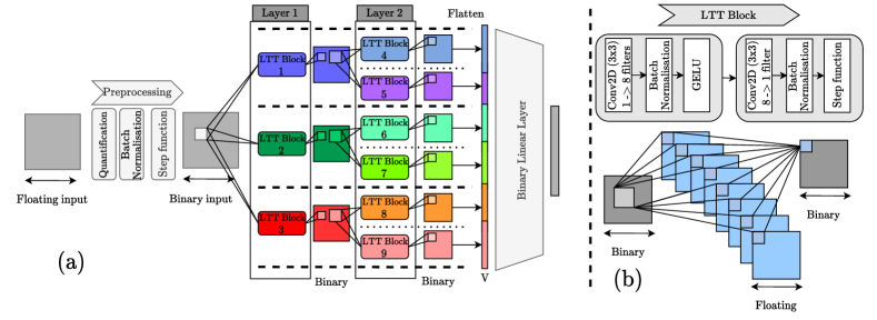
Figure 3: (a) General architecture of the TTnet model with a one-channel input. Layer 0 is a pre-processing layer that allows image binarization. Then follow two layers of Learning Truth Table (LTT) blocks: three blocks in the first layer, six in the second. It should be noted that the LTT block of layer 2 does not take as input all the filters of layer 1, as it is usually the case: it only takes the filter of their groups. Finally, the last linear layer performs the classification. (b) Architecture of a LTT block. It is composed of two layers of grouped 2D-CNN with an expanding factor of 8. It can be seen as an expanding auto-encoder. The intermediate values are real and the input/output values are binary.

Truth Table Deep Convolutional Neural Networks (TTnet) were proposed in (Benamira et al., 2022) as DCNNs convertible into truth tables by design, with security applications (a companion video is provided by the authors https://youtu.be/loGlpVcy0AI). While recent developments in DNN architecture have focused on improving performance, the resulting models have become increasingly complex and difficult to verify, interpret and implement. Thus, the authors focused on CNNs, which are widely used in the field, and tried to transform them into tractable Boolean functions. A depiction of the general architecture of TTnet can be found in Figure 3 of Appendix A.

CNN filter as a tractable Boolean function.

Their proposed method converts CNN filters into binary truth tables by 1) decreasing the input size (noted as $n$ in the rest of the paper) which reduces the complexity of the CNN filter function, 2) using the Heaviside step function denoted as $bin_{act}=(1+sgn(x))/2$ to transform the inputs and outputs into binary values. This results in a tractable Boolean function (for $n$ not too large) that can be stored as a truth table, as seen in Figure 2(a). To achieve high accuracy, the CNN filter must also be non-linear before the step function. Then, the CNN filter becomes a tractable non-linear truth table, which is referred to as a Learning Truth Table (LTT) block.

Description of an LTT block.

Among all the families of LTT blocks possible - we represent in Figure 2(b) an Expanding Auto-Encoder LTT block (E-AE LTT). An E-AE LTT block is composed of two layers of grouped CNN with an expanding factor. Figure 2(a) shows a computation of E-AE 1D LTT block. We can observe that the input size is small ($n=6$), the input/output values are binary and SeLU is an activation function. Note that the inputs are binary but the weights and the intermediate values are real. We integrated LTT blocks into $\mathcal{TT}$net as CNN filters are integrated into DCNNs: each LTT layer is composed of multiple LTT blocks and there are multiple LTT layers in total.

3.4 Challenges and optimizations for integrating TTnet with TFHE-Concrete

The Concrete library (Chillotti et al., 2020b) is a software implementation of TFHE. It is designed to provide a highly efficient and secure platform for performing mathematical operations on Boolean encrypted data. The library utilizes automated operations on lookup tables (concrete-numpy) to achieve high performance while maintaining a high level of security. The library is also designed to be very user-friendly, with simple and intuitive interfaces for performing encryption and decryption operations. The Concrete library has been shown to provide significant improvements in terms of memory and communication overheads compared to other HE schemes. Furthermore, it is open source, which allows researchers and practitioners to easily integrate it into their projects and benefit from its advanced features.

The use of TTnet architecture in combination with TFHE (and more specifically with Concrete) naturally provides a number of advantages. Firstly, the lightweight and differentiable nature of TTnet allows for the implementation of CNNs with direct expressions as truth tables, which is well-suited for Concrete. Additionally, the reduced complexity of the TTnet architecture leads to reduced computations and good scalability. Yet, the integration of TTnet into the TFHE framework presents several challenges that need to be addressed in order to achieve high performance. We detail below the constraints imposed by FHE libraries and the optimizations implemented to overcome these limitations and achieve state-of-the-art performance on various datasets.

Constraints imposed by Concrete.

The Concrete implementation of the TFHE library, which utilizes automated operations on lookup tables, imposes a maximum limit of $16$ on the input bit size $n$ of the truth table. However, $n$ has a strong impact on efficiency (cf Appendix B) and our tests show that $n=4$ or $n=6$ seem to offer the best trade-offs. Indeed, since we learn kernels of convolutional layers of size $(3,2)$ or $(2,3)$, it is convenient to use $n$ a multiple of $2$ and/or $3$. Moreover, input sizes larger than $n=8$ lead to a prohibitive average time per call.

Concrete proposes a built-in linear regression feature, but we tested that it performs not as well as an ad-hoc linear regression with multiplications and additions.

Finally, a very important limitation is that Concrete does not support multi-precision table lookups: the call time of each table lookup (even the small ones) will be equal to the call time of the largest bitwidth operations in the whole circuit. For example, if one of the computations operates on 16 bits, all lookup tables, even small, will require the call time of a 16-bit table lookup. This can be problematic when handling the final linear regression as we will have to sum many Boolean values and the sum result bitwidth might be larger than our planned table lookup size, therefore slowing down our entire implementation. If the sum result of our linear regression requires 16 bits, all our $4$-bit lookup tables call time will be on par with $16$-bit table lookups, going from $75$ms to almost $5$s per call. For now, the computation time is too slow for results that require a sum on more than 4 bits. To overcome this limitation, we implemented several optimizations to improve the accuracy of the model, particularly for image datasets (see below).

Limitations imposed by TTnet.

The original TTnet paper proposed a training method that is not suitable for high accuracy performance as it was trained to resist PGD attacks (Madry et al., 2017), which reduces accuracy. Additionally, the pre-processing and final sparse layers in TTnet being binary, this also leads to a significant decrease in accuracy. To address these limitations, we replace the final sparse binary linear regression with a linear layer with floating point weights (later quantified on 4 bits not to deteriorate too much the performances on Concrete) and propose a new training method that emphasizes accuracy (see below). We also propose to use a setting $N_{1}/{\tt TT}$, where a first layer $N_{1}$ (a layer or block of a general open-source model) is applied to overcome the loss of information due to the first binarization. This is for example a standard method used in BNNs.

Training optimizations.

To improve the accuracy of our model, we took several steps to optimize the training process. First, we removed the use of PGD attacks during training, as they have been shown to reduce accuracy. Next, we employed the DoReFa-Net method (Zhou et al., 2016) for CIFAR-10, a technique for training convolutional neural networks with low-bitwidth activations and gradients. Finally, to overcome the limitations of the TTnet grouping method, we extended the training to 500 epochs, resulting in a more accurate model.

Architectural optimizations.

For tabular datasets, the straightforward enhancements proposed in the previous sections are sufficient to achieve high accuracy. However, this is not the case for image datasets such as MNIST, CIFAR-10, and ImageNet. Therefore, we modify the general architecture of our model. Specifically, we use an architecture similar to the one presented for ImageNet in the original TTnet paper. The limitation of our model is that it can see far in the spatial dimension but has limited representation in the channel dimension. To balance this property, we use three techniques: multi-headers , residual connections (He et al., 2016), and channel shuffling (Zhang et al., 2018). We have a single layer composed of four different functions in parallel: one LTT block with a kernel size of (3,2) and group 1 (to see far in space and low in channel), one LTT block with a kernel size of (2,3) and group 1, one LTT block with a kernel size of 1 and 6 groups (to see low in space but high in channel representation), and an identity function (as a residual connection for stability). We tried with a second layer to increase accuracy, but with the current version of Concrete (without the support of multi-precision table lookups), this led to sub-optimal performance/accuracy trade-offs with a drastic increase in FHE inference time.

Client server usage as optimizations.

We describe here a solution to the issue of Concrete not supporting the results of linear regression that would be on more than 4 bits: we utilize the client’s computing resources not only to prepare the input to the server, but also to post-process the server’s output. Namely, the client will compute a small part of the final linear regression. Indeed, we quantify the weights of the final linear regression of TTnet to 4 bits, which we divide into 4 binary matrices. Then, the server performs partial sums on each of these 4 matrices. Since the outputs of TTnet are binary, the weights are binary, and the maximum number input bitwidth for our lookup tables is 4 bits. For optimal performance, we perform sub-sums of size 16 to ensure that the result of each sub-sum is always lesser than $2^{4}$ as proposed by Zama’s team. It is important to note that by doing this, we maintain the privacy of the weights of the linear regression as they remain unknown to the client. Additionally, the function computation by the client is very light, for example in the case of the MNIST dataset in the ${\tt VGG}_{1B}$/${\tt TT}$ setting, it will represent at most $\frac{N_{\text{features}}}{N_{bits}}=\frac{576}{16}=12$ sums of 4-bit integers to be performed for each $4$ weight matrices. The client will eventually add these four outputs to obtain its final result, i.e. computing $\sum_{i=0}^{3}{2^{i}*w_{i}*\text{output}_{i}}$. Also, note that this client computation is fixed and will remain the same even if the model needs to be updated. Finally, this limitation is due to Concrete and likely temporary as Concrete identified lookup tables multi-precision as an “important feature to come”.

Patching optimizations.

Due to its highly decoupled nature, our model performance is dependent on the number of patches. The classification of an image can be viewed as $N$ independent computations, where $N$ is the number of patches of the original image. This is a unique property and is highly useful for addressing the issue of Concrete requiring a lot of RAM when compiling complex circuits, especially when one will have to scale to larger datasets. For example on MNIST, we have a patch of size (8x8x1) instead of an entire image of size (28x28x1).

4 Results

The project implementation was done in Python, with the PyTorch library (Paszke et al., 2019) for training, in numpy for testing in clear, and the Concrete-numpy library for FHE inference. Our workstation consists of 4 Nvidia GeForce 3090 GPUs (only for training) with 24576 MiB memory and eight cores Intel(R) Core(TM) i7-8650U CPU clocked at 1.90 GHz, 16 GB RAM. For all experiments, the CPU Turbo Boost is deactivated and the processes were limited to using four cores.

The details of all our models’ architecture can be found in Appendix C.

4.1 Tabular datasets

Table 1: Tabular dataset results for TT-TFHE and competitors. All results are in Full-Pr setting. All our models use a table lookup bitwidth of $n=5$, except for Diabetes where we use $n=6$.

	FHE	#CPU	Adult		Cancer		Diabetes
	family	cores	Acc.	Time	Acc.	Time	Acc.	Time
ETHZ/CCS22	CKKS	64	81.6%	420s	-	-	-	-
TAPAS	TFHE	16	-	-	97.1%	3.5s	54.9%	250s
Ours		4	85.3%	5.6s	97.1%	1.9s	57.0%	1.2s

Our experimental results shown in Table 1 (in Table 6 of Appendix F for results normalized to a single CPU) demonstrate the superior performance of the proposed TT-TFHE framework on three tabular datasets (Cancer, Diabetes, Adult) in terms of both accuracy and computational efficiency. The framework achieved an increase in accuracy of up to $+3\%$ compared to state-of-the-art DNN & HE set-ups based on TFHE such as TAPAS (Sanyal et al., 2018) or on CKKS such as the recent work from the ETHZ team (Jovanovic et al., 2022). More impressively, the inference time per CPU was significantly reduced by a factor $1205$x, $7$x, and $825$x on Adult, Cancer, and Diabetes datasets respectively.

This enables the practical deployment of our framework in industrial and real-world scenarios where tabular datasets are prevalent  (Cartella et al., 2021; Buczak & Guven, 2015; Clements et al., 2020; Ulmer et al., 2020; Evans, 2009), with low memory and communication overhead (see Table 5 in Appendix D). Note that these results are in the Full-Pr setting, as the binarization process in TT-TFHE does not lead to any particular issue for tabular datasets.

4.2 Image datasets

Our experimental results and comparisons for image datasets are given in Table 2 (in Table 7 of Appendix F for all results normalized to a single CPU).

Table 2: Image dataset results for TT-TFHE and competitors. Results denoted with * are estimated by the original authors, not measured. All our models use a table lookup bitwidth of $n=4$, except the underlined ones that use $n=6$.

		Full-Pr ($\emptyset$/$N$)				${\tt VGG}_{1B}$/$\emptyset$	${\tt VGG}_{1L}$/$N$		${\tt VGG}_{1B}$/$N$
TFHE-based schemes		TAPAS	GateNet	Zama	Ours	Ours	Zama	Ours	Ours
#CPU cores		16	2	6	4	4	128	4	4
MNIST	Acc. (%)	98.6	98.8*	97.1	97.2	97.5	-	98.2	98.1
	Time	37h	44h*	115s	83.6s	0.04s	-	8.7s	7s
CIFAR-10	Acc. (%)	-	80.5*	-	-	70.4	62.3	69.4/72.1	74.1/75.3
	Time	-	3920h*	-	-	0.4s	29m	9.5m/6.2h	9.5m/6.2h

		Full-Pr ($\emptyset$/$N$)
non-TFHE-based schemes		CryptoNets	Fast CryptoNets	SHE	Lola	Lee et. al.
#CPU cores		4	6	10	8	1
MNIST	Acc. (%)	99	98.7	99.5	99.0	-
	Time	4.2m	39s	9.3s	2.2s	-
CIFAR-10	Acc. (%)	-	76.7	92.5	74.1	91.3
	Time	-	11h	37.6m	12.2m	37.8m

4.2.1 Fully private (Full-Pr) setting

In the Full-Pr configuration, we focused on the performance of our method on the MNIST dataset, as the binarization process in TT-TFHE resulted in a significant loss of accuracy for CIFAR-10 or an increase in inference time. TT-TFHE offers a competitive trade-off compared to other TFHE-based methods, such as TAPAS (Sanyal et al., 2018), GateNet (Fu et al., 2021) or Zama (Chillotti et al., 2021). It is three orders of magnitude faster than TAPAS or GateNet, while showing only a slightly lower accuracy of 1.4%. In comparison to Zama, our method is $2$x faster per CPU for the same level of accuracy. Additionally, we highlight that for our single layer LTT block of size $n=6$, we require 1600 calls to $6$-bit lookup tables, which leads to an inference time of only 83 seconds on four CPU cores.

TT-TFHE is even competitive in terms of inference time with some non-TFHE-based schemes such as (Fast) CryptoNets (Gilad-Bachrach et al., 2016), but can be one order of magnitude slower with slightly lower accuracy. Therefore, one can observe that the Full-Pr setting of TFHE implemented in our framework generally underperforms compared to the very latest Full-Pr CKKS or BFV setups. This is explained by the first binarization process in TT-TFHE, which compresses too much information embedded in the input image. Yet, we again emphasize the many advantages of TFHE-based solutions compared to non-TFHE-based ones: little memory required allowing easy/efficient multi-client inference, low communication overhead, no security warning on TFHE while CKKS secret key can be recovered in polynomial time (Li & Micciancio, 2021) (a fix was proposed afterward  (Li et al., 2022) but not yet implemented in SEAL for example), etc. We will see in the next sub-section that the performance situation is very different in the setting where the client can perform some pre-computation layer.

4.2.2 Other settings

We first observe that when allowing the client to apply a simple pre-processing layer, the performance increases drastically for TT-TFHE. We have implemented and benchmarked both ${\tt VGG}_{1L}/{\tt TT}$ and ${\tt VGG}_{1B}/{\tt TT}$ settings, both with TTnet models with $n=6$ and $n=4$ and we obtained a $10$x performance improvement, with an increase in accuracy. For reference, we have also tested the ${\tt VGG}_{1B}/\emptyset$ setting where only a linear regression is computed privately on server: we remark that adding a TTnet in the server computation indeed improves accuracy by about 4%.

One could argue that more VGG blocks could be computed on client side to further increase the accuracy, but this would reduce the generality of the first layers and lead to PPML solutions that would not adapt very well to multiple use cases. We have tried blocks of other more recent CNNs than VGG, such as DenseNet (Huang et al., 2017), but the results remain very similar.

We can compare the TT-TFHE results to some TFHE-based competitors, as Zama proposed a similar setting with ${\tt VGG}_{1L}$ pre-computed by the client for CIFAR-10, and against which we infer $100$x faster per CPU and with a $10\%$ increase in accuracy.

Our TT-TFHE results are now even competitive against non-TFHE-based solutions (even though they miss many of TFHE advantages), being faster than (Fast) CryptoNets (Gilad-Bachrach et al., 2016) and SHE (Lou & Jiang, 2019), and on par with Lola (Brutzkus et al., 2019) and Lee et. al. (Lee et al., 2022) per CPU. We note that SHE and Lee et. al. have better accuracy than our model.

4.3 Memory/communication cost of TT-TFHE

In Table 5 from Appendix D, we compare the memory and communication needs for all our settings. We can observe that the deeper the representation, the smaller the communication needs: the inputs to the server become smaller as we go deeper into the neural network (there are also fewer computations to do in the server). Some settings do not need public keys as only a linear regression is done, and thus no programmable bootstrapping is involved (Chillotti et al., 2021). Then, the largest the lookup tables (in terms of the number of features and size), the larger will be the public keys as there will be more bootstrapping. Also, the optimization proposed in Section 3.4 to ease the linear regression comes with a cost: it increases the size of the outputs. Indeed, only the ${\tt VGG}_{1B}$/$\emptyset$ setting does not use this optimization as there is no lookup-table involved and thus no bootstrapping. Finally, the encrypted inputs size increases with the number of features.

Comparison with other methods.

As stated in (Clet et al., 2021), CKKS is more memory greedy than TFHE for communication. In Table 4 of Appendix D, we compare between each method the amount of RAM needed on server side for CIFAR-10 dataset. The best accuracy is the ResNet proposed by (Lee et al., 2022), but it also leads to the highest consumption in RAM. With LoLa setting, the accuracy is indeed lower but it requires $32$x lesser RAM. Then, our method reduces again the memory on server by almost a factor of $15$x for the same accuracy. RAM size on server matters for cloud computing as pricing increases along with memory needs, thus low-memory solutions help the scalability of the MLaaS.

5 Limitations and Conclusion

Limitations.

Our proposed framework is still not as performant as the latest non-TFHE-based solutions with regard to running time and accuracy. Moreover, CIFAR-10 and larger datasets remain out of reach for industrial use. Finally, TT-TFHE is for the moment limited by the constraints of the Concrete library.

Conclusion.

In this paper, we presented a new framework, TT-TFHE, which greatly outperforms all TFHE-based PPML solutions in terms of inference time, while maintaining acceptable accuracy. Our proposed framework is a practical solution for real-world applications, particularly for tabular data and small image datasets like MNIST, as it requires minimal memory/communication cost, provides strong security for the client’s data, and is easy to deploy. We believe that this research will spark further investigations into the utilization of truth tables for privacy-preserving data usage, emphasized by the recently NIST Artificial Intelligence Risk Management Framework (AI, 2023).

Appendix

Appendix A General architecture of TTnet

Appendix B On Concrete table lookups

Table 3 presents the average time per call on lookup tables of different sizes for Concrete. We can observe that computation time doubles between $5$-bit and $6$-bit tables. From $8$-bit to $9$-bit, it increases by a factor $3.8$x with almost $3$ seconds for each call. Thus, we focused on tables with a maximum size of $6$ bits. The code used to obtain this table is available on Zama website. Experiments were performed on our CPU, without Turbo Boost.

Table 3: Measured time of a lookup table call through TFHE library Concrete, according to the table input bit sizes.

Input bit size	Average time per call (ms)		Input bit size	Average time per call (ms)
1	49.3		9	2979.5
2	57.6		10	2756
3	57.3		11	3023.2
4	74.6		12	3732.5
5	75.2		13	3956.5
6	169.9		14	4030.1
7	353.4		15	4009.4
8	774.4		16	4499.5

Appendix C Architecture of our models

We detail below the architecture of the various models we use. All the linear regression weights are quantified to 4-bit.

Adult.

This model is composed of one LTT block of kernel size $5$ and stride 4 with no padding. It results in 274 rules being activated, i.e. with weight during linear regression different than $0$.

Cancer.

This model is composed of one LTT block of kernel size $5$ and stride 4 with no padding. It results in 80 rules being activated, i.e. with weight during linear regression different than $0$.

Diabetes.

This model is composed of one LTT block of kernel size $6$ and stride 5 with no padding. It results in 295 rules being activated, i.e. with weight during linear regression different than $0$.

MNIST - Full-Pr.

This model is composed of one LTT block of kernel size $6$ and stride 2 with no padding. The input is resized to $20*20$ before entering the LTT block. It is followed then by a linear layer of $1600$ features to $10$ classes.

MNIST - ${\tt VGG}_{1B}$/$\emptyset$.

This model is composed of the first VGG block followed by a linear layer of $1176$ features to $10$ classes.

MNIST - ${\tt VGG}_{1L}$/TT.

This model is composed of the first VGG block followed by one LTT block of kernel size $2$ and stride 1 with no padding and $24$ channels. It is followed then by a linear layer of $1176$ features to $10$ classes.

MNIST - ${\tt VGG}_{1B}$/TT.

This model is composed of the first VGG block followed by one LTT block of kernel size $2$ and stride 1 with no padding and $16$ channels. It is followed then by a linear layer of $576$ features to $10$ classes.

CIFAR-10 - ${\tt VGG}_{1B}$/$\emptyset$.

This model is composed of the first VGG block followed by a linear layer of $64*11*11=7744$ features to $10$ classes.

CIFAR-10 - ${\tt VGG}_{1L}$/TT.

There are two models for this setup:

• The first model is composed of the first VGG layer followed by three LTT blocks in parallel of kernel size $(2,2)$ and stride 1 with no padding and one residual layer in parallel. The outputs are then concatenated into a vector of size $64*11*11*4=30976$. It is followed then by a linear layer of $30976$ features to $10$ classes.

• The second model is composed of the first VGG layer followed by three LTT blocks and one residual layer all in parallel. The first LTT block uses a kernel size $(3,2)$ and stride 2 with no padding, the second one a kernel size $(2,3)$ and stride 2 with no padding, the third one a kernel size of size $1$ and $6$ groups and stride 2 with no padding. The outputs are then concatenated into a vector of size $64*11*11*4=30976$. It is followed then by a linear layer of $30976$ features to $10$ classes.

CIFAR-10 - ${\tt VGG}_{1B}$/TT.

There are two models for this setup:

• The first model is composed of the first VGG block followed by three LTT blocks in parallel of kernel size $(2,2)$ and stride 1 with no padding and one residual layer in parallel. The outputs are then concatenated into a vector of size $64*11*11*4=30976$. It is followed then by a linear layer of $30976$ features to $10$ classes.

• The second model is composed of the first VGG block followed by three LTT blocks and one residual layer all in parallel. The first LTT block uses a kernel size $(3,2)$ and stride 2 with no padding, the second one a kernel size $(2,3)$ and stride 2 with no padding, the third one a kernel size of size $1$ and $6$ groups and stride 2 with no padding. The outputs are then concatenated into a vector of size $64*11*11*4=30976$. It is followed then by a linear layer of $30976$ features to $10$ classes.

Appendix D On memory/communication costs

We present in Table 4 the reported RAM used of each method. Cryptonets, SHE, Lola and Lee et al. are all Full-Pr, whereas Zama and ours are not as we let the user do one VGG layer or one VGG block locally. We measured the RAM used by Zama on Google Colab with 8 Intel(R) Xeon(R) CPU @ 2.20GHz, and a maximum of 52GB of RAM available. We observe that we use less memory than every proposed method with a competitive accuracy. Only Lee et al. and SHE outperform our accuracy by more than $17\%$ but with huge memory cost: indeed we only need 0.82 GB which is $468\times$ less than Lee et al.. SHE did not report their RAM needs, but they used a 1 TB machine to run their experiments.

Table 4: RAM usage between different methods for the inference of a single image of CIFAR-10. CryptoNets authors did not report results on CIFAR-10, but LoLa team (Brutzkus et al., 2019) estimated that it would take around 100 GBs to infer one image of this dataset with CryptoNets. SHE memory is reported as an upper bound as numbers were not given except for the experimental setup.

Dataset	Method	FHE type	Accuracy	Server RAM
CIFAR-10	CryptoNets	BFV	-	100 GB
	SHE	LTFHE	92.5%	< 1 TB
	LoLa	BFV	74.1%	12 GB
	Lee et al.	CKKS	91.31%	384 GB
	Zama ${\tt VGG}_{1L}$/N	TFHE	62.31%	14.8 GB
	Ours ${\tt VGG}_{1L}$/TT	TFHE	69.4%	0.82 GB
	Ours ${\tt VGG}_{1B}$/TT	TFHE	74.1%	0.82 GB

In Table 5 we report all our memory and communication needs for our TT-TFHE framework. We can observe that we stay relatively low in memory thanks to small lookup tables as the model with lookup tables of bitwidth of $n=6$ need more than $10\times$ the RAM than the model that uses a bitwidth of $n=4$ in exchange for a decrease in accuracy and faster inference time as showed in Table 2.

Table 5: Memory and communication needs for TT-TFHE in various settings. The client will have to send the public keys and the encrypted inputs to the server and then receive the encrypted outputs from it. The communication cost is therefore the sum of these three items. All tabular models use a table lookup bitwidth of $n=5$ and images model a table lookup bitwidth of $n=4$, except for underlined results who use a bitwidth of $n=6$.

		Adult	Cancer	Diabetes	MNIST				CIFAR-10
		Full-Pr	Full-Pr	Full-Pr	Full-Pr	${\tt VGG}_{1B}$/$\emptyset$	${\tt VGG}_{1L}$/TT	${\tt VGG}_{1B}$/TT	${\tt VGG}_{1B}$/$\emptyset$	${\tt VGG}_{1L}$/TT	${\tt VGG}_{1B}$/TT
Client	Encryption Keys	21.6 kB	22 kB	21.6 kB	70.9 kB	10 kB	21.7 kB	21.7 kB	10 kB	21.7 kB / 263.8 kB	21.7 kB / 263.8 kB
	Public Keys	101.6 MB	168.96 MB	101.6 MB	440 MB	0 MB	102 MB	101.9 MB	0 MB	103.0 MB / 3.2 GB	103.0 MB / 3.2 GB
	Encrypted Input Size	4.3 MB	1.2 MB	4.6 MB	100 MB	11.5 MB	18.4 MB	9 MB	75.7 MB	363.2 MB / 5.7 GB	363.2 MB / 5.7 GB
	Encrypted Output Size	1.9 MB	0.5 MB	2.0 MB	220 MB	0.1 MB	40.6 MB	30 MB	0.1 MB	806.6 MB / 12.6 GB	806.6 MB / 12.6 GB
Server	RAM	3.4 MB	1.04 MB	3.4 MB	237.1 MB	0.6 MB	46.13 MB	31.45 MB	0.5 MB	823.1 MB / 10 GB	823.1 MB / 10 GB
Communication Cost (with key)		107.8 MB	170.66 MB	108.2 MB	760 MB	11.6 MB	131 MB	140.9 MB	76.3 MB	1.3 GB / 21.5 GB	1.3 GB / 21.5 GB
Communication Cost (without key)		6.2 MB	1.7 MB	6.6 MB	320 MB	11.6 MB	29 MB	39 MB	76.3 MB	1.2 GB / 18.3 GB	1.2 GB / 18.3 GB

Appendix E Tabular Datasets

All datasets have been split 5 times in a 80-20 train-test split for k-fold testing.

Adult.

The Adult dataset comprises 48,842 individuals, each with 18 binary attributes and a label that indicates whether their income is above or below 50K$ USD or not. The dataset is available at https://archive.ics.uci.edu/ml/datasets/Adult.

Cancer.

The Cancer dataset is composed of 569 data points, each with 30 numerical characteristics. The objective is to predict whether a tumor is malignant or benign. To achieve this, we transformed each integer value into a one-hot vector, resulting in a total of 81 binary features. The dataset is available at https://archive.ics.uci.edu/ml/datasets/Breast+Cancer+Wisconsin+(Diagnostic).

Diabetes.

The Diabetes dataset includes 100000 patient records, each with 50 characteristics that are both categorical and numerical. We retained 43 of these features, 5 of which are numerical, and the rest are categorical. This resulted in 291 binary features and 5 numerical features. The goal is to predict one of the three labels for hospital readmission. The dataset is available at https://archive.ics.uci.edu/ml/datasets/Diabetes+130-US+hospitals+for+years+1999-2008.

Appendix F Comparisons with single-CPU estimations

In this section, we provide the result tables, where the timings have been normalized to a single CPU, for easier comparisons. This scaling seems appropriate as we tested for example that the code produced by Zama for CIFAR-10 in ${\tt VGG}_{1L}$/$N$ setting runs precisely 16 times slower on 8 GPUs than on their benchmark with 128 CPUs.

Table 6: Tabular dataset results for TT-TFHE and competitors. All results are in Full-Pr setting. All our models use a table lookup bitwidth of $n=5$, except for Diabetes where we use $n=6$.

	FHE	#CPU	Adult		Cancer		Diabetes
	family	cores	Acc.	Time	Acc.	Time	Acc.	Time
ETHZ/CCS22	CKKS	1	81.6%	7.5h	-	-	-	-
TAPAS	TFHE	1	-	-	97.1%	56s	54.9%	66m
Ours		1	85.3%	22.4s	97.1%	7.6s	57.0%	4.8s

Table 7: Image dataset results for TT-TFHE and competitors. Results denoted with * are estimated by the original authors, not measured. All our models use a table lookup bitwidth of $n=4$, except the underlined ones that use $n=6$.

		Full-Pr ($\emptyset$/$N$)				${\tt VGG}_{1B}$/$\emptyset$	${\tt VGG}_{1L}$/$N$		${\tt VGG}_{1B}$/$N$
TFHE-based schemes		TAPAS	GateNet	Zama	Ours	Ours	Zama	Ours	Ours
#CPU cores		1	1	1	1	1	1	1	1
MNIST	Acc. (%)	98.6	98.8*	97.1	97.2	97.5	-	98.2	98.1
	Time	592h	88h*	11.5m	5.6m	0.16s	-	34.8s	28s
CIFAR-10	Acc. (%)	-	80.5*	-	-	70.4	62.3	69.4/72.1	74.1/75.3
	Time	-	7840h*	-	-	1.6s	61.8h	38m/24.8h	38m/24.8h

		Full-Pr ($\emptyset$/$N$)
non-TFHE-based schemes		CryptoNets	Fast CryptoNets	SHE	Lola	Lee et. al.
#CPU cores		1	1	1	1	1
MNIST	Acc. (%)	99	98.7	99.5	99.0	-
	Time	16.6m	3.9m	93s	17.6s	-
CIFAR-10	Acc. (%)	-	76.7	92.5	74.1	91.3
	Time	-	66h	6.3h	97m	37.9m

References

- AI (2023) AI, N. Artificial intelligence risk management framework (ai rmf 1.0). 2023.
- Araujo et al. (2019) Araujo, A., Norris, W., and Sim, J. Computing receptive fields of convolutional neural networks. Distill, 2019. doi: 10.23915/distill.00021. https://distill.pub/2019/computing-receptive-fields.
- Benamira et al. (2022) Benamira, A., Peyrin, T., and Kuen-Yew, B. H. Truth-table net: A new convolutional architecture encodable by design into sat formulas, 2022. URL https://arxiv.org/abs/2208.08609.
- Boemer et al. (2019) Boemer, F., Lao, Y., Cammarota, R., and Wierzynski, C. ngraph-he: a graph compiler for deep learning on homomorphically encrypted data. In Proceedings of the 16th ACM International Conference on Computing Frontiers, pp. 3–13, 2019.
- Bourse et al. (2018) Bourse, F., Minelli, M., Minihold, M., and Paillier, P. Fast homomorphic evaluation of deep discretized neural networks. In Annual International Cryptology Conference, pp. 483–512. Springer, 2018.
- Brakerski (2012) Brakerski, Z. Fully Homomorphic Encryption without Modulus Switching from Classical GapSVP. In Safavi-Naini, R. and Canetti, R. (eds.), Advances in Cryptology - CRYPTO 2012 - 32nd Annual Cryptology Conference, Santa Barbara, CA, USA, August 19-23, 2012. Proceedings, volume 7417 of Lecture Notes in Computer Science, pp. 868–886. Springer, 2012. doi: 10.1007/978-3-642-32009-5\_50. URL https://doi.org/10.1007/978-3-642-32009-5_50.
- Brakerski et al. (2014) Brakerski, Z., Gentry, C., and Vaikuntanathan, V. (leveled) fully homomorphic encryption without bootstrapping. ACM Transactions on Computation Theory (TOCT), 6(3):1–36, 2014.
- Brutzkus et al. (2019) Brutzkus, A., Gilad-Bachrach, R., and Elisha, O. Low latency privacy preserving inference. In International Conference on Machine Learning, pp. 812–821. PMLR, 2019.
- Buczak & Guven (2015) Buczak, A. L. and Guven, E. A survey of data mining and machine learning methods for cyber security intrusion detection. IEEE Communications surveys & tutorials, 18(2):1153–1176, 2015.
- Carpov et al. (2015) Carpov, S., Dubrulle, P., and Sirdey, R. Armadillo: a compilation chain for privacy preserving applications. In Proceedings of the 3rd International Workshop on Security in Cloud Computing, pp. 13–19, 2015.
- Cartella et al. (2021) Cartella, F., Anunciacao, O., Funabiki, Y., Yamaguchi, D., Akishita, T., and Elshocht, O. Adversarial attacks for tabular data: Application to fraud detection and imbalanced data. arXiv preprint arXiv:2101.08030, 2021.
- Cheon et al. (2017) Cheon, J. H., Kim, A., Kim, M., and Song, Y. Homomorphic encryption for arithmetic of approximate numbers. In International conference on the theory and application of cryptology and information security, pp. 409–437. Springer, 2017.
- Chillotti et al. (2016) Chillotti, I., Gama, N., Georgieva, M., and Izabachene, M. Faster fully homomorphic encryption: Bootstrapping in less than 0.1 seconds. In international conference on the theory and application of cryptology and information security, pp. 3–33. Springer, 2016.
- Chillotti et al. (2020a) Chillotti, I., Gama, N., Georgieva, M., and Izabachène, M. Tfhe: fast fully homomorphic encryption over the torus. Journal of Cryptology, 33(1):34–91, 2020a.
- Chillotti et al. (2020b) Chillotti, I., Joye, M., Ligier, D., Orfila, J.-B., and Tap, S. Concrete: Concrete operates on ciphertexts rapidly by extending tfhe. In WAHC 2020–8th Workshop on Encrypted Computing & Applied Homomorphic Cryptography, volume 15, 2020b.
- Chillotti et al. (2021) Chillotti, I., Joye, M., and Paillier, P. Programmable bootstrapping enables efficient homomorphic inference of deep neural networks. In International Symposium on Cyber Security Cryptography and Machine Learning, pp. 1–19. Springer, 2021.
- Chou et al. (2018) Chou, E., Beal, J., Levy, D., Yeung, S., Haque, A., and Fei-Fei, L. Faster cryptonets: Leveraging sparsity for real-world encrypted inference. arXiv preprint arXiv:1811.09953, 2018.
- Clements et al. (2020) Clements, J. M., Xu, D., Yousefi, N., and Efimov, D. Sequential deep learning for credit risk monitoring with tabular financial data. arXiv preprint arXiv:2012.15330, 2020.
- Clet et al. (2021) Clet, P.-E., Stan, O., and Zuber, M. Bfv, ckks, tfhe: Which one is the best for a secure neural network evaluation in the cloud? In International Conference on Applied Cryptography and Network Security, pp. 279–300. Springer, 2021.
- Dathathri et al. (2019) Dathathri, R., Saarikivi, O., Chen, H., Laine, K., Lauter, K., Maleki, S., Musuvathi, M., and Mytkowicz, T. Chet: an optimizing compiler for fully-homomorphic neural-network inferencing. In Proceedings of the 40th ACM SIGPLAN Conference on Programming Language Design and Implementation, pp. 142–156, 2019.
- Ducas & Micciancio (2015) Ducas, L. and Micciancio, D. Fhew: bootstrapping homomorphic encryption in less than a second. In Annual international conference on the theory and applications of cryptographic techniques, pp. 617–640. Springer, 2015.
- Evans (2009) Evans, D. S. The online advertising industry: Economics, evolution, and privacy. Journal of economic perspectives, 23(3):37–60, 2009.
- Fan & Vercauteren (2012) Fan, J. and Vercauteren, F. Somewhat Practical Fully Homomorphic Encryption. IACR Cryptol. ePrint Arch., pp. 144, 2012. URL http://eprint.iacr.org/2012/144.
- Fu et al. (2021) Fu, C., Huang, H., Chen, X., and Zhao, J. Gatenet: Bridging the gap between binarized neural network and fhe evaluation. In ICLR Workshop on Security and Safety in Machine Learning Systems, 2021.
- Gentry (2009) Gentry, C. Fully homomorphic encryption using ideal lattices. In Proceedings of the forty-first annual ACM symposium on Theory of computing, pp. 169–178, 2009.
- Gilad-Bachrach et al. (2016) Gilad-Bachrach, R., Dowlin, N., Laine, K., Lauter, K., Naehrig, M., and Wernsing, J. Cryptonets: Applying neural networks to encrypted data with high throughput and accuracy. In International conference on machine learning, pp. 201–210. PMLR, 2016.
- He et al. (2016) He, K., Zhang, X., Ren, S., and Sun, J. Deep residual learning for image recognition. In Proceedings of the IEEE conference on computer vision and pattern recognition, pp. 770–778, 2016.
- Huang et al. (2017) Huang, G., Liu, Z., Van Der Maaten, L., and Weinberger, K. Q. Densely connected convolutional networks. In Proceedings of the IEEE conference on computer vision and pattern recognition, pp. 4700–4708, 2017.
- Jovanovic et al. (2022) Jovanovic, N., Fischer, M., Steffen, S., and Vechev, M. Private and reliable neural network inference. In Proceedings of the 2022 ACM SIGSAC Conference on Computer and Communications Security, pp. 1663–1677, 2022.
- Juuti et al. (2019) Juuti, M., Szyller, S., Marchal, S., and Asokan, N. Prada: protecting against dnn model stealing attacks. In 2019 IEEE European Symposium on Security and Privacy (EuroS&P), pp. 512–527. IEEE, 2019.
- Juvekar et al. (2018) Juvekar, C., Vaikuntanathan, V., and Chandrakasan, A. GAZELLE: A low latency framework for secure neural network inference. In 27th USENIX Security Symposium (USENIX Security 18), pp. 1651–1669, 2018.
- Krizhevsky et al. (2017) Krizhevsky, A., Sutskever, I., and Hinton, G. E. Imagenet classification with deep convolutional neural networks. Communications of the ACM, 60(6):84–90, 2017.
- Lee et al. (2022) Lee, E., Lee, J.-W., Lee, J., Kim, Y.-S., Kim, Y., No, J.-S., and Choi, W. Low-complexity deep convolutional neural networks on fully homomorphic encryption using multiplexed parallel convolutions. In International Conference on Machine Learning, pp. 12403–12422. PMLR, 2022.
- Li & Micciancio (2021) Li, B. and Micciancio, D. On the security of homomorphic encryption on approximate numbers. In Annual International Conference on the Theory and Applications of Cryptographic Techniques, pp. 648–677. Springer, 2021.
- Li et al. (2022) Li, B., Micciancio, D., Schultz, M., and Sorrell, J. Securing approximate homomorphic encryption using differential privacy. In Advances in Cryptology–CRYPTO 2022: 42nd Annual International Cryptology Conference, CRYPTO 2022, Santa Barbara, CA, USA, August 15–18, 2022, Proceedings, Part I, pp. 560–589. Springer, 2022.
- Li et al. (2017) Li, L. E., Chen, E., Hermann, J., Zhang, P., and Wang, L. Scaling machine learning as a service. In International Conference on Predictive Applications and APIs, pp. 14–29. PMLR, 2017.
- Lou & Jiang (2019) Lou, Q. and Jiang, L. She: A fast and accurate deep neural network for encrypted data. Advances in Neural Information Processing Systems, 32, 2019.
- Madry et al. (2017) Madry, A., Makelov, A., Schmidt, L., Tsipras, D., and Vladu, A. Towards deep learning models resistant to adversarial attacks. arXiv preprint arXiv:1706.06083, 2017.
- Mishra et al. (2020) Mishra, P., Lehmkuhl, R., Srinivasan, A., Zheng, W., and Popa, R. A. Delphi: A cryptographic inference service for neural networks. In 29th USENIX Security Symposium (USENIX Security 20), pp. 2505–2522, 2020.
- Paszke et al. (2019) Paszke, A., Gross, S., Massa, F., Lerer, A., Bradbury, J., Chanan, G., Killeen, T., Lin, Z., Gimelshein, N., Antiga, L., Desmaison, A., Kopf, A., Yang, E., DeVito, Z., Raison, M., Tejani, A., Chilamkurthy, S., Steiner, B., Fang, L., Bai, J., and Chintala, S. Pytorch: An imperative style, high-performance deep learning library. In Advances in Neural Information Processing Systems 32, pp. 8024–8035. Curran Associates, Inc., 2019.
- Philipp et al. (2020) Philipp, R., Mladenow, A., Strauss, C., and Völz, A. Machine learning as a service: Challenges in research and applications. In Proceedings of the 22nd International Conference on Information Integration and Web-based Applications & Services, pp. 396–406, 2020.
- Podschwadt et al. (2022) Podschwadt, R., Takabi, D., Hu, P., Rafiei, M. H., and Cai, Z. A survey of deep learning architectures for privacy-preserving machine learning with fully homomorphic encryption. IEEE Access, 10:117477–117500, 2022.
- Regulation (2016) Regulation, P. Regulation (eu) 2016/679 of the european parliament and of the council. Regulation (eu), 679:2016, 2016.
- Ribeiro et al. (2015) Ribeiro, M., Grolinger, K., and Capretz, M. A. Mlaas: Machine learning as a service. In 2015 IEEE 14th International Conference on Machine Learning and Applications (ICMLA), pp. 896–902. IEEE, 2015.
- Sanyal et al. (2018) Sanyal, A., Kusner, M., Gascon, A., and Kanade, V. Tapas: Tricks to accelerate (encrypted) prediction as a service. In International Conference on Machine Learning, pp. 4490–4499. PMLR, 2018.
- Simonyan & Zisserman (2014) Simonyan, K. and Zisserman, A. Very deep convolutional networks for large-scale image recognition. arXiv preprint arXiv:1409.1556, 2014.
- Tramèr et al. (2016) Tramèr, F., Zhang, F., Juels, A., Reiter, M. K., and Ristenpart, T. Stealing machine learning models via prediction APIs. In 25th USENIX security symposium (USENIX Security 16), pp. 601–618, 2016.
- Ulmer et al. (2020) Ulmer, D., Meijerink, L., and Cinà, G. Trust issues: Uncertainty estimation does not enable reliable ood detection on medical tabular data. In Machine Learning for Health, pp. 341–354. PMLR, 2020.
- Zhang et al. (2018) Zhang, X., Zhou, X., Lin, M., and Sun, J. Shufflenet: An extremely efficient convolutional neural network for mobile devices. In Proceedings of the IEEE conference on computer vision and pattern recognition, pp. 6848–6856, 2018.
- Zhou et al. (2016) Zhou, S., Wu, Y., Ni, Z., Zhou, X., Wen, H., and Zou, Y. Dorefa-net: Training low bitwidth convolutional neural networks with low bitwidth gradients. arXiv preprint arXiv:1606.06160, 2016.