A new dynamical modeling of the WASP-47
system with CHEOPS observations

Among the hundreds of known hot Jupiters (HJs), only five have been found to have companions on short-period orbits. Within this rare class of multiple planetary systems, the architecture of WASP-47 is unique, hosting an HJ (planet -b) with both an inner and an outer sub-Neptunian mass companion (-e and -d, respectively) as well as an additional non-transiting, long-period giant (-c). The small period ratio between planets -b and -d boosts the transit time variation (TTV) signal, making it possible to reliably measure the masses of these planets in synergy with the radial velocity (RV) technique. In this paper, we present new space- and ground-based photometric data of WASP-47b and WASP-47-d, including 11 unpublished light curves from the ESA mission CHaracterising ExOPlanet Satellite (CHEOPS). We analyzed the light curves in a homogeneous way together with all the publicly available data to carry out a global $N$-body dynamical modeling of the TTV and RV signals. We retrieved, among other parameters, a mass and density for planet -d of $M_{\mathrm{d}}=15.5\pm 0.8$ $M_{\oplus}$ and $\rho_{\mathrm{d}}=1.69\pm 0.22$ g cm^-3, which is in good agreement with the literature and consistent with a Neptune-like composition. For the inner planet (-e), we found a mass and density of $M_{\mathrm{e}}=9.0\pm 0.5$ $M_{\oplus}$ and $\rho_{\mathrm{e}}=8.1\pm 0.5$ g cm^-3, suggesting an Earth-like composition close to other ultra-hot planets at similar irradiation levels. Though this result is in agreement with previous RV plus TTV studies, it is not in agreement with the most recent RV analysis (at 2.8$\sigma$), which yielded a lower density compatible with a pure silicate composition. This discrepancy highlights the still unresolved issue of suspected systematic offsets between RV and TTV measurements. In this paper, we also significantly improve the orbital ephemerides of all transiting planets, which will be crucial for any future follow-up.

1 Introduction

Hot Jupiters (HJs), that is, giant, gaseous planets ($0.3\lesssim M_{\mathrm{p}}\lesssim 13$ $M_{\mathrm{jup}}$) orbiting their host stars on very short orbits ($P\lesssim 10$ d), have been the subject of many “firsts” in the history of exoplanetary research, as the first planet discovered around a solar-type star (51 Peg b; Mayor & Queloz 1995) is an HJ and the first reported transiting planet (HD 209458 b; Charbonneau et al. 2000; Henry et al. 2000), which is also the first planet where an atmospheric feature has been detected (Charbonneau et al. 2002), is an HJ. Although 479 HJs have been discovered so far by various techniques, albeit mostly by combining transit photometry and radial velocity (RV) measurements, many key questions are still unanswered about their formation, migration, and successive evolution (Dawson & Johnson, 2018; Fortney et al., 2021).

Table 1: Mass measurements of the WASP-47 planets published in the literature.

Reference	$M_{\textrm{e}}/M_{\oplus}$	$M_{\textrm{b}}/M_{\oplus}$	$M_{\textrm{d}}/M_{\oplus}$	$M_{\textrm{c}}\sin i/M_{\oplus}$	Method
Hellier et al. (2012)	—	$364\pm 16$	—	—	RV
Neveu-VanMalle et al. (2016)	—	$360\pm 19$	—	$396\pm 70$	RV
Dai et al. (2015)	$12.2\pm 3.7$	$370\pm 29$	$10.4\pm 8.4^{\dagger}$	—	RV
Becker et al. (2015)	$<22^{\ddagger}$	$341^{+73}_{-55}$	$15\pm 7$	—	RV+TTV
Almenara et al. (2016)	$9.1^{+1.8}_{-2.9}$	$364\pm 8$	$15.7\pm 1.1$	$361^{+80}_{-54}$	RV+TTV¶
Weiss et al. (2017)	$9.1\pm 1.0$	$358\pm 12$	$13.6\pm 2.0$	$416\pm 16$	RV+TTV
Sinukoff et al. (2017)	$9.1\pm 1.2$	$356\pm 12$	$12.7\pm 2.7$	$411\pm 18$	RV
Vanderburg et al. (2017)	$6.8\pm 0.7$	$363\pm 7$	$13.1\pm 1.5$	$398\pm 9$	RV§
Bryant & Bayliss (2022)	$6.8\pm 0.6$	$364\pm 7$	$14.2\pm 1.3$	$399\pm 9$	RV§
This work (see also Table 11)	$9.0\pm 0.5$	$374\pm 17$	$15.5\pm 0.8$	$447\pm 20$	RV+TTV

Hundreds of multiple planetary systems have been detected with space-based missions such as Convection, Rotation and planetary Transits (CoRoT; Auvergne et al. 2009), Kepler/K2 (Borucki et al., 2010; Ricker et al., 2015), and the Transiting Exoplanet Survey Satellite (TESS; Ricker et al. 2015). These systems show great diversity in their architecture, with planets spanning the full range of planetary masses and being arranged in very different dynamical configurations. However, HJs have been known for a long time to be preferentially lonely when compared to other classes (Latham et al., 2011; Huang et al., 2016; Steffen et al., 2012), and almost all their known companions are long-period massive planets at $P\gtrsim 200$ d detected through either modulation or long-term trends in their RVs (Knutson et al., 2014). The rarity of HJ companions with inner or short-period orbits has been confirmed by a recent global analysis of TESS photometry by Hord et al. (2021). There are only a handful of notable examples of HJs with nearby companions: WASP-47, the subject of this paper (see below), Kepler-730 (Zhu et al., 2018; Cañas et al., 2019), TOI-1130 (Huang et al., 2020), WASP-132 (Hord et al., 2022), and the most recently reported TOI-2000 (Sha et al., 2021). Together, these five planets represent less than $1\%$ of the known HJs. Notably, WASP-47 is unique among the mentioned systems for showing clear transit time variations (TTVs), allowing researchers to jointly exploit TTVs and RVs to measure the planetary masses and other orbital parameters in a much more reliable way than using the two techniques separately (Malavolta et al., 2017).

WASP-47 has been dubbed “the gift that keeps on giving” (Kane et al., 2020) due to the many layers of scientific investigation it has stimulated. The first member of this planetary system, HJ WASP-47b ($1.14\pm 0.02$ $M_{\mathrm{jup}}$, $1.127\pm 0.013$ $R_{\mathrm{jup}}$, $P\simeq 4.159$ d) was discovered by Hellier et al. (2012) from ground-based photometric data (SuperWASP). A few years later, WASP-47 was observed by K2 during its Campaign 3, enabling the detection of two additional companions (Becker et al., 2015): WASP-47e ($6.8\pm 0.7$ $M_{\oplus}$, $1.81\pm 0.03$ $R_{\oplus}$, $P\simeq 0.789$ d), an inner super-Earth, and WASP-47d ($13.1\pm 1.5$ $M_{\oplus}$, $3.58\pm 0.05$ $R_{\oplus}$, $P\simeq 9.031$ d), an outer Neptunian. Around the same time, the results from the first extensive RV campaign (Neveu-VanMalle et al., 2016) revealed the presence of a fourth non-transiting Jupiter-sized planet on a much longer orbit, WASP-47c ($1.25\pm 0.03$ $M_{\mathrm{jup}}$, $P\simeq 588$ d). Subsequent RV analysis with fresh data have further refined and/or constrained the planetary masses (Dai et al., 2015; Sinukoff et al., 2017; Vanderburg et al., 2017). The opportunity of combining TTV and RV analysis in a joint approach was exploited by Almenara et al. (2016) and Weiss et al. (2017), the former within a photodynamical framework. All the published measurements of planetary masses for WASP-47 are summarized in Table 2. It is worth mentioning that the measurement of the spin-orbit angle obtained through the Rossiter-McLaughlin effect is consistent with an aligned configuration ($\lambda=0^{\circ}\pm 24^{\circ}$) for WASP-47b (Sanchis-Ojeda et al., 2015) and that a phase-curve re-analysis of K2 photometry constrained the WASP-47b albedo to values significantly lower than the average of HJs (Kane et al., 2020). Lastly, a very recent analysis by Bryant & Bayliss (2022) focusing on the characterization of planet -e has made use of both TESS and ESPRESSO data for the first time.

Despite the extensive amount of work carried out on WASP-47 so far, a convincing and complete description of the evolutionary history of this system is still elusive. Our current understanding of this system will change once the James Webb Space Telescope (JWST) enables a detailed atmospheric characterization of WASP-47’s transiting planets, especially of the small ones: -e and -d (Bryant & Bayliss, 2022). Unfortunately, a reasonably accurate prediction of the future transits of planet -d is difficult, as even the best available ephemerides based on a combination of K2 and RV data will have drifted by about one hour (1-$\sigma$) at epoch 2023.0. The photometric detection of WASP-47d is indeed beyond the reach of ground-based facilities, and TESS has been unable to significantly detect the only transit predicted to fall in Sector 42 (and will not re-observe it at least until the end of Cycle 6 in 2024). The need to recover a new set of reliable ephemerides is one of the initial motivations of our investigation. In addition, the mass measurements of planet -d and -e have historically been slightly inconsistent with each other due to a small statistical tension between the most precise estimate through a photodynamical approach and studies wholly based on RV data (Table 2). Although the most recent ESPRESSO measurements (Bryant & Bayliss, 2022) appear to have solved this tension for planet -d (but still not for -e), WASP-47 remains one of the very few systems for which a precise mass measurement can be achieved by either TTVs or RVs, potentially shedding some light on an old debate about a possible systematic discrepancy between the two techniques (Mills & Mazeh, 2017; Petigura et al., 2018).

In this paper, we present new data from the CHaracterising ExOPlanet Satellite (CHEOPS) and new ground-based photometric data for WASP-47b and WASP-47d, and we perform a global dynamical re-analysis of all the available data, including the latest TESS and ESPRESSO data sets. We focus particularly on the determination of the orbital and physical parameters of planet -d and -e in order to address the aforementioned issues. In Section 2, we describe all the photometric and spectroscopic data analyzed in this work. In Section 3, we deal with the light curve fitting and the dynamical modeling. Finally, we present and discuss our results, including a comparison with the literature, in Section 4.

2 Observations

For our dynamical analysis, we gathered all the publicly available RV and photometric data of WASP-47. This included both public data (from K2, TESS, and several RV surveys) and new proprietary data from CHEOPS and ground-based telescopes, described below. A log summarizing all the analyzed photometric data is reported in the Appendix. The time stamps associated with all the measurements were consistently converted to the $\textrm{BJD}_{\textrm{TDB}}$ standard, as prescribed by Eastman et al. (2010).

2.1 CHEOPS photometry

Launched in 2019, CHEOPS (Benz et al., 2021) is an ESA S-class mission currently carrying out its 3.5-year nominal observing program. The scientific instrument of CHEOPS is a 32-cm reflecting telescope designed to deliver defocused images for the performance of ultra high-precision photometric measurements of bright stars. The high-performance capabilities of CHEOPS when working with transit timing in particular have been demonstrated by Borsato et al. (2021).

Eleven visits of WASP-47 were scheduled with CHEOPS in 2020 and 2021 within the Guaranteed Time Observations (GTO) programs CH_PR100017 and CH_PR100025 (see Table 8 for a list of the CHEOPS data sets). Ten visits were centered on the transits of WASP-47b (Table 13), and one was centered on WASP-47d (Table 15). All the light curves were extracted from the raw satellite data by the official CHEOPS Data Reduction Pipeline v13.1 (DRP; Hoyer et al. 2020), and their plots are shown in the left panel of Fig. 1 (planet -b) and in Fig. 3 (planet -d). The exposure time was set to 60 s and the minimum efficiency to 50%, resulting in some of the light curves showing noticeable gaps every 98.77 min (the orbital period of CHEOPS) due to the spacecraft crossings of the South Atlantic Anomaly as well as Earth-related constraints (blockage of the line-of-sight by the Earth and high levels of stray light).

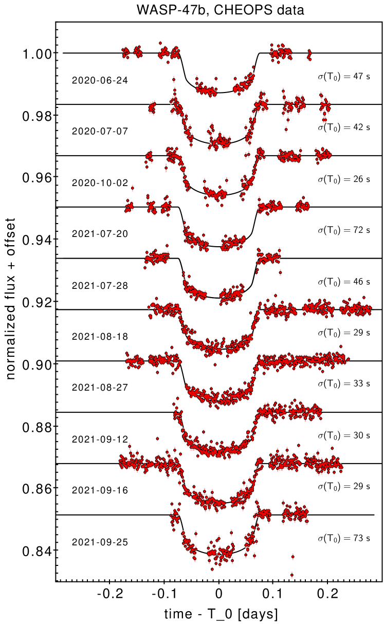
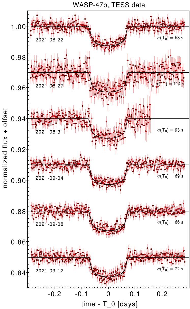
Figure 1: Space-based light curves of WASP-47b from CHEOPS and TESS analyzed for the present work after de-trending. For each light curve, the corresponding label shows the acquisition date in UT and the timing error $\sigma_{T_{0}}$ (in seconds). Arbitrary vertical offsets of 0.0165 and 0.03 were added, respectively, to both sets for visualization purposes.

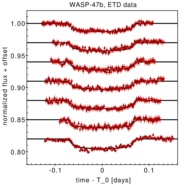
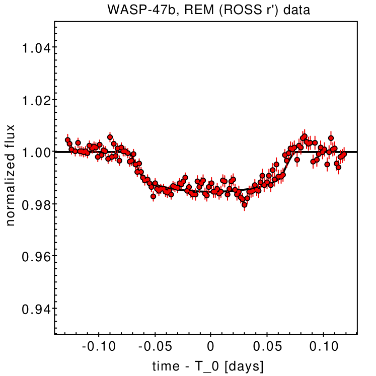
Figure 2: Ground-based light curves of WASP-47b from ETD and REM analyzed for the present work. An arbitrary vertical offset of 0.03 was added to the ETD light curves for visualization purposes. The light curves are sorted in chronological order (see Table 14) increasing towards bottom.

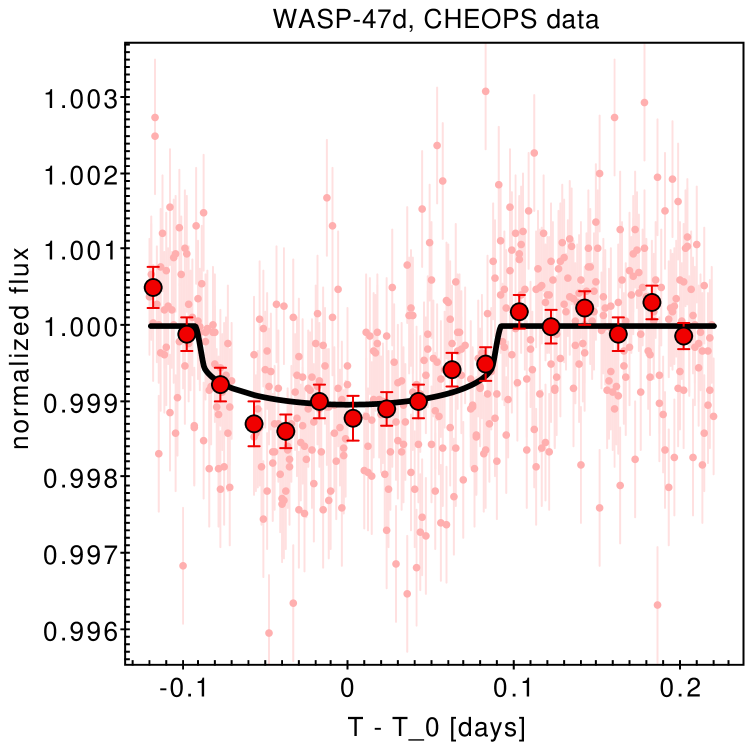
Figure 3: CHEOPS light curve of WASP-47d after de-trending. The pink data points are at the original sampling cadence (60 s), and the red circles were averaged over 20-min intervals.

2.2 K2 and TESS photometry

During its Campaign 3, K2 monitored WASP-47 in short-cadence mode (net cadence: 58.3 s) for 69 nearly uninterrupted days, from November 14, 2014, to January 23, 2015. These data sets were used to study the transits of planets -d and -e for the first time (Becker et al., 2015). We also use their light curves in our analysis, as they are already corrected for jitter-induced systematic errors by fitting splines as a function of spatial drift, following the procedure by Vanderburg & Johnson (2014). Overall, 108 transit light curves from K2 were ingested in our analysis: 16 of planet -b, seven of planet -d, and 85 of planet -e. These are summarized in Table 13, 15, and 16-17, respectively.

Almost seven years later, WASP-47 was observed by TESS for the first time (and the only time so far) in Sector 42 (camera 1, CCD 4), from August 20 to September 16, 2021. Being a known planet host, it was designated as a 120-s cadence target. The resulting data set is the same investigated by Bryant & Bayliss (2022), who used of the Pre-search Data Conditioned Simple Aperture Photometry (PDCSAP) light curve made available by the Science Processing Operations Center (SPOC) pipeline (Jenkins et al., 2016). Unfortunately, the PDCSAP light curve is missing a large one-week section, including two transits of WASP-47b (on August 27 and 31), due to a “scattered light” quality flag. Unlike Bryant & Bayliss (2022), we based our analysis on Simple Aperture Photometry (SAP) data, where the two missing transits are preserved and do not appear to be impacted by a significant amount of systematic noise, as is demonstrated in Section 3.1. While the SAP algorithm does not correct the light curves for photometric dilution due to contaminating sources, we emphasize that no Gaia DR3 source (limiting magnitude $G\simeq 21$) is present at all within a radius of $30^{\prime\prime}$ from WASP-47, and the brightest one within $60^{\prime\prime}$ has $G=17.50$, implying a negligible dilution factor. We also note that a constant dilution factor does not have any systematic effect on the measurement of transit times because it does not alter the symmetry of the transit signal.

Overall, six TESS light curves of planet -b (Table 13; right panel of Fig. 1) were ingested. As already noted by Bryant & Bayliss (2022), individual transits from planet -d and -e are hidden in the TESS photometric scatter, and their detection is at most marginal. Our preliminary fitting tests confirmed this, and we did not attempt to retrieve their timings. The next visit to WASP-47 by TESS is not expected until at least the end of Cycle 6 (October 2024).

2.3 Ground-based photometry

One transit of WASP-47b was observed on September 24, 2021, by the 60-cm Rapid-Eye Mount telescope (REM; Zerbi et al. 2001) through the ROS2 instrument (Molinari et al., 2014), a charge-coupled device (CCD) camera able to observe the same field of view ($9.1^{\prime}\times 9.1^{\prime}$) simultaneously in four photometric bands (Sloan $g^{\prime}$, $r^{\prime}$, $i^{\prime}$, and $z^{\prime}$). These observations (PI: Nascimbeni) were carried out as part of the TASTE program, a ground-based multi-site long-term TTV campaign to monitor transiting planets (Nascimbeni et al., 2011). Two bright reference stars (TYC 5805-338-1 and TYC 5805-739-1) were always imaged along with the target, allowing us to perform differential photometry. In addition, in order to mitigate systematic errors from guiding drifts, pixel-to-pixel non-homogeneity, and flat-field errors, a generous amount of defocus was applied ($\textrm{FWHM}\gtrsim 10$ pix).

The four transit light curves from the observation were extracted by running STARSKY (Nascimbeni et al., 2013), the photometric pipeline developed for TASTE. The STARSKY pipeline automatically selects the best combination of photometric aperture radii and weighting scheme to minimize the final out-of-transit scatter. No linear detrending against the external parameters automatically tested by STARSKY proved to be effective (i.e., linear baseline, airmass, $x$-$y$ position, background level, stellar FWHM). Guiding drifts unfortunately turned out to be much larger than anticipated, totaling more than 30 pixels throughout the whole series. The resulting systematic errors impacted the $g^{\prime}$, $i^{\prime}$, and $z^{\prime}$ data to an unacceptable extent, while the $r^{\prime}$ light curve was mostly spared, thanks to its much better flat-field correction and its structure being more homogeneous at small spatial scales. For this reason, we only considered the $r^{\prime}$ light curve (right panel of Fig. 2) for our subsequent analysis.

Seven additional transit light curves of WASP-47b (of six distinct transit events) were collected from 2020 to 2021 by Y. Jongen and A. Wünsche and are available on the public archive of the Exoplanet Transit Database (ETD; Poddaný et al. 2010). They were gathered through an $R$ filter with a PlaneWave CDK 17” telescope coupled with a Moravian G4 16k CCD camera at the Deep Sky Chile facility (Jongen) and with an unfiltered PlaneWave CDK 20” telescope coupled with the same camera at the El Sauce Observatory in Chile (Wünsche). The exposure time was set to 120 s by both observers. After visually checking their quality and converting the time stamps to $\textrm{BJD}_{\textrm{TDB}}$, the transit light curves were included in our analysis as well. These light curves are detailed in Table 14 and plotted in the left panel of Fig. 2.

2.4 Radial velocities

We collected all the available high-precision RV data for our analysis from the scientific literature:

• 19 from ESPRESSO (Bryant & Bayliss, 2022),

• 47 from HIRES (Sinukoff et al., 2017),

• 69 from HARPS-N (Vanderburg et al., 2017),

• 26 from PFS (Dai et al., 2015),

• 51 from CORALIE (Hellier et al., 2012; Neveu-VanMalle et al., 2016),

for a total of 212 independent data points spanning nine years (2010-2019).

3 Data analysis

Table 2: Stellar and limb darkening parameters adopted in the transit fitting process (Section 3.1) and subsequent dynamical analysis (Section 3.2).

Stellar parameters
Mass ($M_{\odot}$)		$1.058\pm 0.047$
Radius ($R_{\odot}$)		$1.156\pm 0.009$
Limb darkening parameters
Instrument	$u_{1}$	$u_{2}$
CHEOPS	$0.571\pm 0.020$	$0.096\pm 0.044$
REM ($r$)	$0.558\pm 0.023$	$0.112\pm 0.054$
TESS	$0.444\pm 0.016$	$0.120\pm 0.038$
K2	$0.562\pm 0.020$	$0.102\pm 0.044$
ETD	$0.558\pm 0.023$	$0.112\pm 0.054$

3.1 Light curve fitting

All the photometric data described in the previous section were homogeneously (re-)analyzed through the PyORBIT (Malavolta et al., 2016, 2018) code. The CHEOPS light curves also went through an additional detrending stage using cheope, an optimized python tool (of which pycheops is the back-end; Maxted et al. 2022) specifically developed to filter, correct, and fit CHEOPS data. The detrending model of cheope is defined as a linear combination of terms, including a quadratic baseline $f_{0}+\mathrm{d}f/\mathrm{d}t+\mathrm{d}^{2}f/\mathrm{d}t^{2}$, the first and second order derivative of the centroid offset in $x$ and $y$ pixel coordinates ($\mathrm{d}f/\mathrm{d}x$, $\mathrm{d}^{2}f/\mathrm{d}x^{2}$, $\mathrm{d}f/\mathrm{d}y$, $\mathrm{d}^{2}f/\mathrm{d}y^{2}$), background ($\mathrm{d}f/\mathrm{d}b$), contamination ($\mathrm{d}f/\mathrm{d}\textrm{contam}$), and the first three harmonics of the spacecraft roll angle (in $\cos\phi$ and $\sin\phi$). There is also an additional term called “glint” that empirically models the internal reflections as a spline-based smooth function (Borsato et al., 2021). The combination of terms to be adopted as the best detrending model was selected automatically by cheope according to its Bayes factor, first through an lmfit optimization (Newville et al., 2014) to find a reasonable starting point and then with an emcee fit (Foreman-Mackey et al., 2013).

For both CHEOPS and all the other data sets, the stellar activity signal and any residual instrumental trend were subtracted using wōtan (Hippke et al., 2019) after masking the transits of planets -b, -d, and -e to get the normalized light curves. The filter adopted was a Tukey’s bi-weight with a window filter duration set equal to the transit duration plus its 1-$\sigma$ uncertainty. All the detrended transits from ground- and space-based telescopes are shown in Figs. 1, 2, and 3. As for the TESS Sector 42 light curves, we focused our analysis on the extraction of six transits of planet -b only, after masking the transits of planets -d and -e, which were only marginally detectable in this data set and hence not usable for an individual $T_{0}$ fit.

In order to extract the central transit times $T_{0}$, we applied PyORBIT independently on each of the five data sets (i.e., CHEOPS, TESS, K2, REM, and ETD), performing a modeling of each light curve using PyDE+emcee (Parviainen et al., 2016; Foreman-Mackey et al., 2013). We assumed Keplerian orbits for all three fitted planets, -b, -e, and -d. We fixed the $a/R_{\star}$ parameter of each planet at the values found on the highest S/N data set (K2; Vanderburg et al. 2017), leaving the individual $T_{0}$ values, the planetary radius $R_{\mathrm{p}}/R_{\star}$, and the orbital inclination $i$ for each planet as the only free parameters in order to take into account changes in the impact parameter as a function of time or different transit depths through different instruments and filters. The stellar parameters were derived by the CHEOPS Stellar Characterization team following the procedure described by Borsato et al. (2022), Section 3.2.1. The two parameters that are crucial for our dynamical analysis, the stellar radius ($R_{\odot}$) and mass ($M_{\odot}$), are listed in Table 6. We adopted a quadratic law $u_{1}$, $u_{2}$ for the limb darkening coefficients, but we re-parameterized them as fitting parameters $q_{1}$ and $q_{2}$ , as done by Kipping (2013). The priors set on the coefficients $u_{1}$ and $u_{2}$ are reported in Table 6. We assumed a Gaussian prior distribution over the coefficients for all the instruments using a bi-linear interpolation of the limb-darkening profile defined in Claret (2017, 2021).

We used PyDE to find the best starting point for the MCMC sampler. For each data set, PyDE used a population size of $4\times N_{par}$, where $N_{par}$ is the number of free parameters, and let it evolve for $64\,000$ generations, and for the Bayesian sampler, we set 100 chains for $150\,000$ steps, discarding the first $40\,000$ by adopting a thinning factor of 100. All the final $T_{0}$ values of this analysis are summarized in Tables 13 to 17 of Appendix References, while the physical best-fit values of the common parameters among individual data sets ($R_{\mathrm{p}}$, $i$) are shown in Table 8. As anticipated in Section 2, we directly compared the transit timings we extracted from TESS SAP photometry with those obtained from the PDCSAP light curves by Bryant & Bayliss (2022) and listed in their Table 4 to check for any systematic offset. The average $\Delta T_{0}=T_{0,\textrm{PDCSAP}}-T_{0,\textrm{SAP}}$ evaluated over the four transits in common yielded 14 s (with average error bars of $\sim 66$ s), and no pair disagreed by more than 0.5 $\sigma$. In other words, timings from SAP and PDCSAP are in perfect statistical agreement.

Table 3: Best-fit values of planetary radius $R_{\mathrm{p}}$ (derived from $R_{\mathrm{p}}/R_{\star}$) and orbital inclination $i$. All these parameters were fitted as common parameters among individual data sets.

Parameter	WASP-47b	WASP-47d	WASP-47e
CHEOPS
$R_{\mathrm{p}}\,(R_{\oplus})$	$12.72\pm 0.12$	$\phantom{0}3.88\pm 0.20$	–
$i$ (∘)	$89.21\pm 0.51$	$89.23\pm 0.51$	–
TESS
$R_{\mathrm{p}}\,(R_{\oplus})$	$12.61\pm 0.17$	–	–
$i$ (∘)	$88.6\pm 0.6$	–	–
K2
$R_{\mathrm{p}}\,(R_{\oplus})$	$12.86\pm 0.10$	$\phantom{0}3.65\pm 0.03$	$\phantom{0}1.83\pm 0.02$
$i$ (∘)	$89.00\pm 0.17$	$89.23\pm 0.10$	$86.73\pm 1.76$
ETD
$R_{\mathrm{p}}\,(R_{\oplus})$	$12.95\pm 0.17$	–	–
$i$ (∘)	$89.06\pm 0.58$	–	–
REM
$R_{\mathrm{p}}\,(R_{\oplus})$	$13.64\pm 0.28$	–	–
$i$ (∘)	$87.86\pm 0.45$	–	–

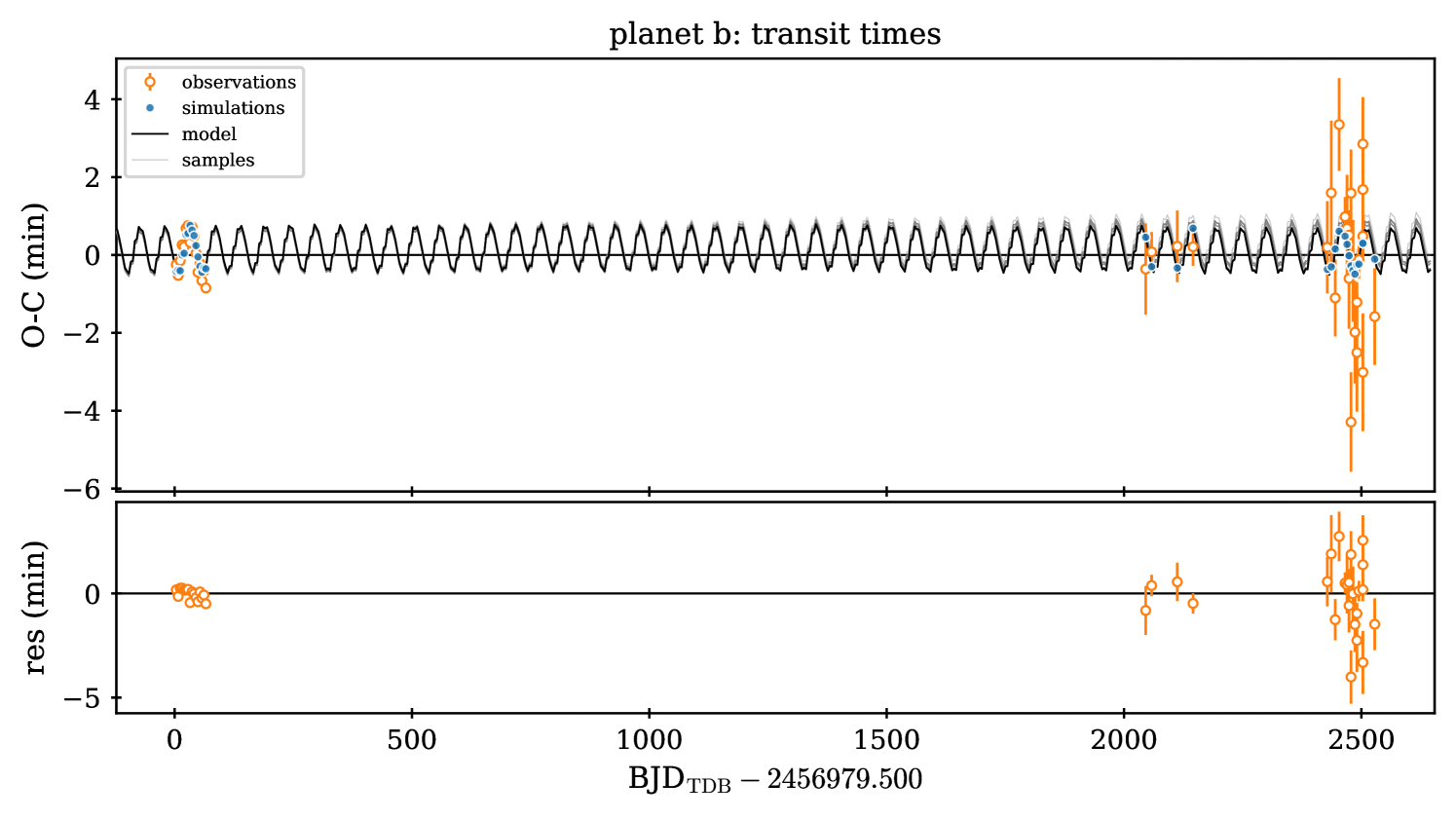
Figure 4: Transit times of WASP-47b. Upper panel: Observed - Calculated $(O-C)$ diagram. The $O-C$ was calculated by subtracting the predicted $T_{0}$ calculated from the linear ephemeris to the observed transit times. The $O-C$ values computed from the observed $T_{0}$s are plotted as open orange circles, while the $O-C$ of the TRADES-simulated $T_{0}$s from the best-fit model are plotted as blue circles. Samples drawn from the posterior distribution within HDI are shown as grey lines. Lower panel: Residuals computed as the difference between observed and simulated $T_{0}$s.

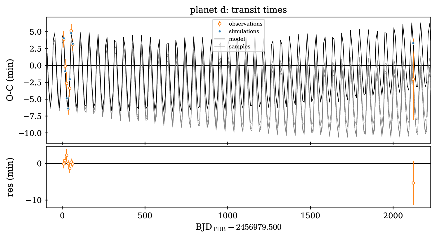
Figure 5: Transit times of WASP-47d. Upper panel: Observed - Calculated $(O-C)$ diagram. The $O-C$ was calculated by subtracting the predicted $T_{0}$ calculated from the linear ephemeris to the observed transit times. The $O-C$ values computed from the observed $T_{0}$s are plotted as open orange circles, while the $O-C$ of the TRADES-simulated $T_{0}$s from the best-fit model are plotted as blue circles. Samples drawn from the posterior distribution within HDI are shown as grey lines. Lower panel: Residuals computed as the difference between observed and simulated $T_{0}$s.

3.2 Dynamical modeling

We employed the TRADES dynamical integrator (Borsato et al., 2014), which has already been successfully applied to Kepler/K2 (Borsato et al., 2019) and CHEOPS data (Borsato et al., 2021) as well as to simulate the Ariel TTV science case (Borsato et al., 2022). The TRADES dynamical integrator allowed us to fit transit times ($T_{0}$) and RVs simultaneously during the integration of the orbits. We fitted the mass ratios ($M_{\mathrm{p}}/M_{\star}$), the periods ($P$), and the mean longitude ($\lambda$) for all the planets. The eccentricity ($e$) and the argument of periastron ($\omega$) were fitted as ($\sqrt{e}\cos\omega,\sqrt{e}\sin\omega$) for planets -b, -c, and -d, while we used the (initial) circular orbit ($e=0$, $\omega=90^{\circ}$) for planet -e due to its extremely short tidal circularization timescale (Vanderburg et al., 2017). We adopted our initial values for $M_{b}$, $M_{c}$, $M_{d}$, $M_{e}$, $e$ and $\omega$ from Almenara et al. (2016). We fixed the longitude of the ascending node ($\Omega$) of -b, -c, and -e to $180^{\circ}$. For the orbital inclination $i$, we took the weighted average of the fitted values from Section 3.1 and Table 8 (for instance, $i_{\mathrm{b}}=88.88\pm 0.14^{\circ}$). We found that by assuming $i_{\mathrm{d}}<90^{\circ}$, one of the most recent transits of planet -b was missed by our integration (i.e., the impact parameter for that transit was greater than one). Almenara et al. (2016) reported a best-fit inclination higher than $90^{\circ}$, but the authors specified that the supplementary angle is equally probable. If both planets -b and -d transit in the same stellar hemisphere (with respect to the observer’s line of sight), then their relative distance would be shorter with respect to the case with planet -d on the opposite hemisphere. The mutual gravitational interaction would of course be much stronger in the former case, moving planet -b on some occasions to a non-transiting configuration that is not observed in our data. Therefore, we assumed that planet -d transits the opposite hemisphere with respect to -b ($i_{\mathrm{b}}<90^{\circ}$) and adopted the value $180^{\circ}-i_{\mathrm{d}}$ as the initial parameter for TRADES. We also fitted the $i$ and $\Omega$ of -d, and we set $i_{\mathrm{c}}$ to $90^{\circ}$. All the orbital parameters are astrocentric and defined at the reference time $2456979.5\,\mathrm{BJD_{TDB}}$, the same as in Almenara et al. (2016). The initial periods were set to the linear ephemeris fitted to $T_{0}$s determined in Section 3.1. For each RV data set, we fitted a $\log_{2}$-based jitter and an RV offset ($\gamma$). However, we found that changing the starting point of the jitter (e.g., $\log_{2}$ of 0.5 and $<1\times 10^{-6}\,\mathrm{ms^{-1}}$) did not affect the final distribution of the chains and, therefore, did not change the best-fit solution. We split the CORALIE data set into three subsets, as done in Almenara et al. (2016), for a total of seven RV data sets. In all, we fitted 34 parameters, all with uniform-uninformative priors in the parameter space.

In order to save computational time, we first ran a local minimizer and used the result as a starting point for the python package emcee (Foreman-Mackey et al., 2013, 2019), for which we initialized 68 walkers with a tight Gaussian. We adopted as a sampler algorithm a mix of the differential evolution proposal (80% of the walkers; Nelson et al., 2014) and the snooker differential evolution proposal (20% of the walkers; ter Braak & Vrugt, 2008). We let the code run for 110 000 steps and discarded the first 100 000 steps as burn-in after checking the convergence of the chains by means of visual inspection as well as through diagnostics from Geweke 1991 (within $2$-$3\sigma$) and Gelman-Rubin statistics (Gelman & Rubin, 1992). Our uncertainties are computed as the high density interval (HDI) at $68.27\%$ from the posterior distribution as the equivalent of the credible intervals at the $16$th and $84$th percentile. We defined our best-fit solution as the maximum likelihood estimator (MLE), that is, the parameter sample that maximizes the log-likelihood ($\log\mathcal{L}$) of the posterior distribution within the HDI. We also computed a symmetric uncertainty ($\sigma$) as the $68.27$th percentile of the (sorted) absolute residuals of the posterior with respect to the best-fit solution. (See Table 11 for a summary of the fitted and physical parameters of the system determined with TRADES. See the O-C diagrams of planet -b, -d, and -e in Figs. 4, 5, and 6 and the RV plot in Fig 7.)

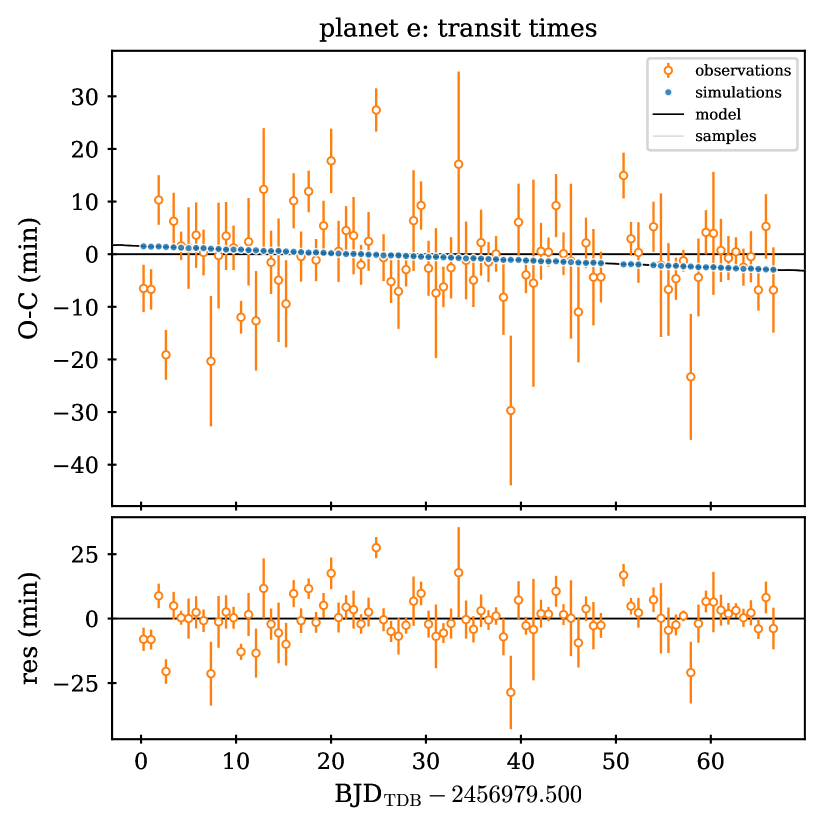
Figure 6: Transit times of WASP-47e. Elements are the same as in Figs. 4 and 5, but for planet -e.

Figure 7: Radial velocities of WASP-47. Upper panel: RV plot. There is a different marker and color for each data set. The TRADES best-fit RV model is plotted with open black shapes. The maximum-likelihood orbital solution is shown by a light gray line. The CORALIE data set was divided into three data sets, as described in Almenara et al. (2016). Lower panel: RV residuals with respect to the TRADES RV best-fit model. The corresponding jitter determined from the best-fit model has been added in quadrature to the measured uncertainty of each data point.

Table 4: Summary of the best-fit MLE parameters for the WASP-47 system determined with TRADES.

parameter (unit)	MLE (HDI & $\sigma$)	priors
planet b
$M_{\mathrm{p}}/M_{\star}\,(M_{\odot}/M_{\star}\times 10^{-3})$	$1.0617_{-0.0007}^{+0.0015}\pm 0.0012$
$P$ (days)	$4.158548_{-0.000017}^{+0.000008}\pm 0.000013$	$\mathcal{U}(3.8,4.5)$
$\sqrt{e}\cos\omega$	$0.0005_{-0.0091}^{+0.0042}\pm 0.007$
$\sqrt{e}\sin\omega$	$0.0239_{-0.004}^{+0.009}\pm 0.007$
$\lambda\,(^{\circ})$	$329.05_{-0.01}^{+0.03}\pm 0.02$	$\mathcal{U}(0,360)$
$M_{\mathrm{p}}\,(M_{\oplus})$	$374_{-16}^{+17}\pm 17$	$\mathcal{U}(80,636)$
$e$	$0.0006_{-0.0002}^{+0.0005}\pm 0.0004$	$\mathcal{U}(0.0,0.5)$
$\omega\,(^{\circ})$	$89_{-11}^{+19}\pm 17$	$\mathcal{U}(0,360)$
$\mathcal{M}\,(^{\circ})$	$60_{-19}^{+11}\pm 17$	$\mathcal{U}(0,360)$
planet c
$M_{\mathrm{p}}/M_{\star}\,(M_{\odot}/M_{\star}\times 10^{-3})$	$1.270_{-0.017}^{+0.005}\pm 0.012$
$P$ (days)	$589.57_{-0.02}^{+0.02}\pm 0.02$	$\mathcal{U}(560,600)$
$\sqrt{e}\cos\omega$	$-0.19060_{-0.02}^{+0.00001}\pm 0.015$
$\sqrt{e}\sin\omega$	$0.478_{-0.016}^{+0.007}\pm 0.014$
$\lambda\,(^{\circ})$	$166.02_{-0.01}^{+0.03}\pm 0.02$	$\mathcal{U}(0,360)$
$M_{\mathrm{p}}\,(M_{\oplus})$	$447_{-22}^{+18}\pm 20$	$\mathcal{U}(159,636)$
$e$	$0.264_{-0.012}^{+0.007}\pm 0.011$	$\mathcal{U}(0.0,0.5)$
$\omega\,(^{\circ})$	$111.8_{-0.2}^{+2.7}\pm 2$	$\mathcal{U}(0,360)$
$\mathcal{M}\,(^{\circ})$	$234.3_{-2.7}^{+0.2}\pm 2$	$\mathcal{U}(0,360)$
planet d
$M_{\mathrm{p}}/M_{\star}\,(M_{\odot}/M_{\star}\times 10^{-3})$	$0.0440_{-0.0017}^{+0.0007}\pm 0.0013$
$P$ (days)	$9.09577_{-0.00008}^{+0.00016}\pm 0.00013$	$\mathcal{U}(8.7,9.3)$
$\sqrt{e}\cos\omega$	$0.0037_{-0.0115}^{+0.0017}\pm 0.009$
$\sqrt{e}\sin\omega$	$0.031_{-0.006}^{+0.016}\pm 0.012$
$\lambda\,(^{\circ})$	$278.61_{-0.01}^{+0.04}\pm 0.03$	$\mathcal{U}(0,360)$
$i\,(^{\circ})$	$90.805_{-0.014}^{+0.020}\pm 0.018$	$\mathcal{U}(80,100)$
$\Omega\,(^{\circ})$	$179.954_{-0.012}^{+0.006}\pm 0.010$	$\mathcal{U}(0,360)$
$M_{\mathrm{p}}\,(M_{\oplus})$	$15.5_{-0.9}^{+0.7}\pm 0.8$	$\mathcal{U}(1,159)$
$e$	$0.0010_{-0.0007}^{+0.0008}\pm 0.0008$	$\mathcal{U}(0.0,0.5)$
$\omega\,(^{\circ})$	$83_{-3}^{+18}\pm 14$	$\mathcal{U}(0,360)$
$\mathcal{M}\,(^{\circ})$	$16_{-15}^{+10}\pm 14$	$\mathcal{U}(0,360)$
planet e
$M_{\mathrm{p}}/M_{\star}\,(M_{\odot}/M_{\star}\times 10^{-3})$	$0.0254_{-0.0003}^{+0.0010}\pm 0.0008$
$P$ (days)	$0.789608_{-0.000001}^{+0.000002}\pm 0.000001$	$\mathcal{U}(0.7,0.86)$
$\lambda\,(^{\circ})$	$149.074_{-0.033}^{+0.015}\pm 0.03$	$\mathcal{U}(0,360)$
$M_{\mathrm{p}}\,(M_{\oplus})$	$9.0_{-0.4}^{+0.6}\pm 0.5$	$\mathcal{U}(1,80)$
$\mathcal{M}\,(^{\circ})$	$244.15_{-0.033}^{+0.015}\pm 0.025$	$\mathcal{U}(0,360)$
RV data-sets
$\gamma_{\mathrm{CORALIE1}}\,(\mathrm{ms^{-1}})$	$-27069_{-2}^{+3}\pm 2$
$\gamma_{\mathrm{CORALIE2}}\,(\mathrm{ms^{-1}})$	$-27084.9_{-4.2}^{+0.4}\pm 3.2$
$\gamma_{\mathrm{CORALIE3}}\,(\mathrm{ms^{-1}})$	$-27065_{-2}^{+8}\pm 6$
$\gamma_{\mathrm{PFS}}\,(\mathrm{ms^{-1}})$	$17.80_{-0.09}^{+1.20}\pm 0.8$
$\gamma_{\mathrm{HIRES}}\,(\mathrm{ms^{-1}})$	$4.6_{-0.6}^{+0.2}\pm 0.5$
$\gamma_{\mathrm{HARPS}}\,(\mathrm{ms^{-1}})$	$-27041.1_{-0.3}^{+0.4}\pm 0.3$
$\gamma_{\mathrm{ESPRESSO}}\,(\mathrm{ms^{-1}})$	$-27165.7_{-0.5}^{+0.1}\pm 0.3$

4 Discussion and conclusions

The global analysis presented in this work is the most comprehensive dynamical modeling of the WASP-47 planetary system carried out so far. We exploited all the available RV and TTV data sets and merged them with 19 unpublished light curves, 11 of which were observed with CHEOPS. Our newly derived planetary masses ($M_{b}$, $M_{c}$, $M_{d}$, and $M_{e}$) from the final best-fit parameters (Table 11) can be compared with the values reported in the literature and listed in Table 2.

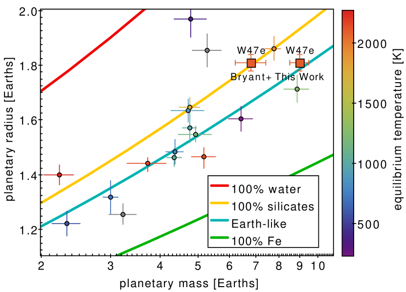
Figure 8: Mass-radius diagram with all the known planets with a relative error on bulk density better than 20% (circle points) color coded according to their equilibrium temperature. The colored lines represent models at different bulk compositions from Zeng et al. (2019). The two measurements of WASP-47e by us and by Bryant & Bayliss (2022) are plotted as squares.

For the two low-mass planets (-d, -e), we found best-fit masses ($M_{d}/M_{\oplus}=15.5\pm 0.8$, $M_{e}/M_{\oplus}=9.0\pm 0.5$) with relative errors of about 5%, which is smaller than all the previous relative errors and is now limited mostly by our knowledge of the stellar mass (relative error on $M_{\star}$: $\sim$4%). In particular, for the innermost planet, our solution is perfectly consistent with the upper extreme $M_{e}/M_{\oplus}=9.1\pm 1.0$ set by Weiss et al. 2017 (joint RV plus TTV analysis), but it is not consistent with the lower extreme $M_{e}/M_{\oplus}=6.8\pm 0.6$ set by Bryant & Bayliss 2022 using RVs only, apparently confirming, at 2.8$\sigma$ significance, some kind of systematic offset between the two techniques (Mills & Mazeh, 2017; Petigura et al., 2018). We did not see a similar behavior for planet -d, whose best-fit mass is fully consistent with all the previous measurements but more precise. By calculating the bulk densities as derived quantities from Table 11 and propagating the errors, we get $\rho_{\mathrm{d}}=1.69\pm 0.22\,\mathrm{g\,cm^{-3}}$ and $\rho_{\mathrm{e}}=8.1\pm 0.5\,\mathrm{g\,cm^{-3}}$, thus confirming a Neptune-like density and composition for planet -d (implying an extended volatile envelope) but also moving planet -e very close to what planetary structure models predict to be an Earth-like composition rather than a pure-silicate one (in contrast to the claims by Vanderburg et al. 2017 and Bryant & Bayliss 2022; see Fig. 8). If that conclusion were true, then planet -e would not appear as an outlier in the planetary density versus stellar irradiation diagram anymore and there would be no reason to hypothesize a different formation path with respect to other ultra-short period planets at similar irradiation levels, such as K2-141b and HD 213885b (Malavolta et al., 2018; Espinoza et al., 2020). Moreover, WASP-47 is a rather metal-rich star at $\textrm{[Fe/H]}=+0.36\pm 0.05$, according to Mortier et al. (2013). The high density of WASP-47e, which fits into the “super-Mercury” class, would confirm the finding by Adibekyan et al. (2021) that the bulk density of super-Earths correlates with stellar iron fraction. On the other hand, the relatively low density of planet -d would also confirm the trend discovered by Wilson et al. (2022), who found that sub-Neptunes around metal-rich stars have, on average, lower densities. Taken together, our findings would support the general idea that a higher stellar metallicity leads to forming planets with larger cores and, hence, generates denser hot super-Earths (such as -e) and warm sub-Neptunes that are able to retain more extended atmospheric envelopes (-d).

We caution, however, that the existing tension on $M_{\mathrm{e}}$ could be due to subtle methodological biases in RV and/or RV plus TTV analyses that are yet to be fully explored and a deeper understanding of the effects at play in such dynamically complex systems is needed. This is true of course for not only WASP-47 but for all planetary systems for which both techniques can be applied and that are steadily growing in number, especially after the launch of K2 and TESS. Two factors are most frequently discussed when dealing with such issues: the impact of stellar activity and the way RV and TTV information is merged at the analysis stage. Notably, WASP-47 is not a particularly active star, and all the studies up to and including Vanderburg et al. (2017) explicitly neglected any contribution from stellar activity on both photometric and spectroscopic data. Bryant & Bayliss (2022), on the other hand, noticed an excess scatter in the ESPRESSO data and concluded that the inclusion of a Gaussian process kernel in their RV modeling was justified by a lower BIC value of their fit, even though the statistical significance of the peak on the periodogram of the RV residuals at the claimed rotational period is marginal. The treatment of stellar activity, however, does not appear to be the (only) explanation for the $M_{\mathrm{e}}$ discrepancy we see since Bryant & Bayliss (2022) came to a value that is almost identical to that reported by Vanderburg et al. (2017) without modeling for it: $M_{\mathrm{e}}=6.8\pm 0.7$ vs. $6.8\pm 0.6$ $M_{\oplus}$. Beyond that, in an RV plus TTV study such ours, it is extremely difficult to model stellar activity in a consistent framework because the two techniques are effected in different ways and at different timescales (Boisse et al., 2011; Oshagh et al., 2013; Ioannidis et al., 2016); indeed, transit light curves are impacted more by the local rather than global distribution of star spots over the photosphere. With WASP-47, an additional issue prevents us from adopting a more complicated data model (i.e., including stellar activity and/or a photodynamical approach): computational time. Having to deal with four planets, 34 free parameters, and an extensive set of 133 transits and 212 RVs, each of the MCMC steps of the optimization process described in Section 3.2 took about 15 s on a medium-power computing workstation, and the whole fit required weeks to reach convergence. This sizable computing time is mostly due to an unfortunate combination of a very long observing baseline (15 years) and the very short period of the inner planet ($P_{\mathrm{e}}\simeq 0.79$ d), forcing the N-body integration time step to unusually small values. Of course, under these assumptions, the inclusion of a Gaussian process treatment of stellar activity or, even worse, the implementation of a photodynamical algorithm would increase the computational time up to an unreasonable amount, at least with ordinarily available hardware. We emphasize, however, that our result agrees with previous RV plus TTV studies both based (Almenara et al., 2016) and not based (Weiss et al., 2017) on a photodynamical approach, so fitting our light curves and performing the dynamical modeling at separate stages cannot be the sole reason for the discrepancy discussed above.

As for the giant planets (-b and -c), it is worth noting that our newly derived masses are compatible with those presented by Vanderburg et al. (2017) and Bryant & Bayliss (2022) and statistically consistent with all the previous measurements reported in Table 2. The precision of our values $M_{b}/M_{\oplus}=374\pm 17$, $M_{c}/M_{\oplus}=447\pm 20$ is larger by a factor of about two with respect to the most recent RV works. This is easily understood if we consider that our error on $M_{\star}$ ($4.4\%$) is larger than theirs (3%) and our dynamical analysis probes are $M_{\mathrm{p}}/M_{\star}$ rather than $M_{\mathrm{p}}/M_{\star}^{2/3}$, the latter being true for a pure RV analysis. In other words, our study is more sensitive to the uncertainty on stellar mass. The same is true for the derived planetary density $\rho_{\mathrm{b}}=0.98\pm 0.09$ $\mathrm{g\,cm^{-3}}$.

An important byproduct of our analysis is the derivation of new, updated mean ephemerides for all the WASP-47 transiting planets, as this data can be exploited by any future follow-up study. Our best-fit relations are:

$$T_{\mathrm{0,b}} = 2459407.761987\pm 0.0000002\textrm{ BJD}_{\textrm{TDB}}$$

$$+N\times(4.159151\pm 0.0000004),$$

$$T_{\mathrm{0,d}} = 2457024.430107\pm 0.0000003\textrm{ BJD}_{\textrm{TDB}}$$

$$+N\times(9.030501\pm 0.000013),$$

$$T_{\mathrm{0,e}} = 2457012.13666\pm 0.00003\textrm{ BJD}_{\textrm{TDB}}$$

$$+N\times(0.78961\pm 0.00003),$$

where $N$ is an integer number commonly known as “epoch” and set arbitrarily to zero at our reference transit time $T_{\mathrm{ref}}$. We highlight that the 1$\sigma$ uncertainty on transit prediction at 2023.0 for planet -d has now been reduced from about one hour to just six minutes. Of course this is crucial for planning space-based observations, where the cost of the invested observing time and the time-sensitive nature of the observations makes pinpointing the transit window as precisely as possible critical.

Observations of WASP-47 are not yet scheduled with JWST, at least during Cycle 1, even though its transiting planets -e, -b, and -d have been recognized as suitable targets for transmission spectroscopy (Bryant & Bayliss, 2022) and will very likely be proposed in the next cycles. Such observations will be crucial to test our planetary formation theories. It is widely accepted that three main channels for HJ migration exist (Dawson & Johnson, 2018): one is through the protoplanetary disk at low eccentricity, another is through high-eccentricity dynamical migration with tidal damping at later times, and the third is through in situ formation close to or at the final orbit. A planet migrating through the disc or having formed in situ would accrete a large amount of gas from inside the ice line, whereas an HJ that migrated dynamically may have originated from beyond the ice line with a different composition (Öberg et al., 2011; Madhusudhan et al., 2017; Knierim et al., 2022). Simulations show that the dynamical migration channel would invariably destroy any close-in planets, as the orbit of the HJ would intersect with that of the close-in planets prior to circularization (Mustill et al., 2015). Thus, unlike ordinary HJs, for very rare systems such as WASP-47, we can rule out one of the main scenarios and test the other models through detailed atmospheric characterization.

Other space-based follow-up opportunities include, at least in principle, TESS, PLATO (Rauer et al., 2014), and ARIEL (Tinetti et al., 2018). As for TESS, we mentioned in the introduction that no other sector will include WASP-47, at least up to the end of Cycle 6, implying that this target will not be re-observed until fall 2024, at best. Unfortunately, individual transits of planets -e and -d are essentially undetectable by TESS due to its noise properties, and the time baseline of each sector is limited to about four weeks. Future sectors, if any, will thus not be effective in significantly extending the TTV analysis carried out so far.

On the other hand, PLATO will be able to deliver high-precision transit light curves of planets -e and -d since the predicted noise level ranges from 90 to 180 ppm in one hour, according to the number of co-pointing PLATO cameras involved (Montalto et al., 2021). Due to its very low ecliptic latitude, WASP-47 will not lie within the proposed Long-duration Observing Phase fields of PLATO (Nascimbeni et al., 2022), where targets will be continuously observed for at least two years. However, WASP-47 could be selected for the Short-duration Observing Phase and monitored for two to three months without any significant interruption (see Fig. 1 of Heller et al. 2022).

As a closing note, ARIEL, though focused on the atmospheric characterization of exoplanets through emission and transmission spectroscopy (Tinetti et al., 2021), has also been proposed as a very powerful instrument to investigate TTVs (Borsato et al., 2022). WASP-47 is consistently included in the provisional ARIEL target list (Zingales et al., 2018; Edwards & Tinetti, 2022) as a “Tier 2” object (aim: in-depth atmospheric characterization through repeated observations), but these observations are only devoted to observing eclipses of planet -b.

Appendix A Data tables

Transits of planets WASP-47b, WASP-47d, WASP-47e fitted in the present work (Section 3.1) and included in our global dynamical analysis (Section 3.2).

Table 5: Transits of planet WASP-47b from space-based telescopes included in our global analysis.

source	UT date	N	cadence	$\sigma_{\mathrm{phot}}$	$T_{0}$	$\sigma(T_{0})$	$\sigma(T_{0})$
(+ band)	(of $T_{0}$)		(s)	(ppm)	($\mathrm{BJD_{TDB}}$)	(days)	(s)
CHEOPS	2020-06-24	242	60	1050	2459025.11931	0.00054	47
CHEOPS	2020-07-07	251	60	1960	2459037.59764	0.00048	42
CHEOPS	2020-10-02	283	60	1190	2459124.93989	0.00031	26
CHEOPS	2021-07-20	271	60	1130	2459416.08220	0.00083	72
CHEOPS	2021-07-28	236	60	1140	2459424.39829	0.00053	46
CHEOPS	2021-08-18	522	60	1270	2459445.19505	0.00033	29
CHEOPS	2021-08-27	537	60	1140	2459453.51274	0.00038	33
CHEOPS	2021-09-12	357	60	1220	2459470.14844	0.00035	30
CHEOPS	2021-09-16	512	60	1390	2459474.30828	0.00034	29
CHEOPS	2021-09-25	247	60	2630	2459482.62705	0.00085	73
TESS	2021-08-22	412	120	2150	2459449.35394	0.00079	68
TESS	2021-08-27	411	120	3900	2459453.51314	0.00132	114
TESS	2021-08-31	319	120	3330	2459457.66953	0.00107	93
TESS	2021-09-04	412	120	2040	2459461.83102	0.00080	69
TESS	2021-09-08	411	120	2040	2459465.98830	0.00076	66
TESS	2021-09-12	412	120	2110	2459470.14753	0.00083	72
K2	2014-11-21	741	60	347	2456982.97692	0.00043	37
K2	2014-11-25	754	60	342	2456987.13597	0.00008	7
K2	2014-11-29	821	60	357	2456991.29538	0.00008	7
K2	2014-12-03	732	60	342	2456995.45461	0.00022	19
K2	2014-12-08	740	60	349	2456999.61388	0.00009	8
K2	2014-12-12	833	60	348	2457003.77342	0.00008	7
K2	2014-12-16	739	60	352	2457007.93265	0.00008	7
K2	2014-12-20	709	60	354	2457012.09155	0.00043	37
K2	2014-12-24	709	60	362	2457016.25091	0.00008	7
K2	2014-12-28	828	60	354	2457020.40989	0.00008	7
K2	2015-01-02	449	60	361	2457024.56863	0.00037	32
K2	2015-01-06	728	60	361	2457028.72772	0.00008	7
K2	2015-01-10	729	60	362	2457032.88682	0.00008	7
K2	2015-01-14	860	60	346	2457037.04569	0.00008	7
K2	2015-01-18	741	60	352	2457041.20502	0.00008	7
K2	2015-01-22	739	60	345	2457045.36340	0.00041	36

Table 6: Transits of planet WASP-47b from ground-based telescopes included in our global analysis.

source	UT date	N	cadence	$\sigma_{\mathrm{phot}}$	$T_{0}$	$\sigma(T_{0})$	$\sigma(T_{0})$
(+ band)	(of $T_{0}$)		(s)	(ppm)	($\mathrm{BJD_{TDB}}$)	(days)	(s)
REM ($g^{\prime}$)	2021-09-25	137	60	3002	2459482.61821	0.00197	171
REM ($r^{\prime}$)	2021-09-25	139	60	2119	2459482.62461	0.00106	91
REM ($i^{\prime}$)	2021-09-25	139	60	2672	2459482.62212	0.00145	125
ETD ($R$)	2020-08-30	145	60	1315	2459091.66670	0.00064	56
ETD ($R$)	2021-07-12	144	60	1581	2459407.76213	0.00082	71
ETD ($R$)	2021-08-06	141	60	1658	2459432.71923	0.00081	70
ETD ($R$)	2021-08-31	155	60	1617	2459457.67291	0.00077	67
ETD ($R$)	2021-09-25	147	60	1540	2459482.62786	0.00073	63
ETD (clear)	2021-09-25	142	60	1723	2459482.62868	0.00084	72
ETD ($R$)	2021-10-20	129	60	1730	2459507.58050	0.00085	74

Table 7: Transits of planet WASP-47d included in our global analysis.

source	UT date	N	cadence	$\sigma_{\mathrm{phot}}$	$T_{0}$	$\sigma(T_{0})$	$\sigma(T_{0})$
(+ band)	(of $T_{0}$)		(s)	(ppm)	($\mathrm{BJD_{TDB}}$)	(days)	(s)
CHEOPS	2020-06-24	242	60	1050	2459025.11931	0.00054	47
K2	2014-11-21	741	60	347	2456982.97692	0.00043	37
K2	2014-11-25	754	60	342	2456987.13597	0.00008	7
K2	2014-11-29	821	60	357	2456991.29538	0.00008	7
K2	2014-12-03	732	60	342	2456995.45461	0.00022	19
K2	2014-12-08	740	60	349	2456999.61388	0.00009	8
K2	2014-12-12	833	60	348	2457003.77342	0.00008	7
K2	2014-12-16	739	60	352	2457007.93265	0.00008	7
K2	2014-12-20	709	60	354	2457012.09155	0.00043	37
K2	2014-12-24	709	60	362	2457016.25091	0.00008	7
K2	2014-12-28	828	60	354	2457020.40989	0.00008	7
K2	2015-01-02	449	60	361	2457024.56863	0.00037	32

Table 8: CHEOPS data sets used in our analysis.

CH_PR100025_TG005601_V0200      CH_PR100025_TG005602_V0200      CH_PR100017_TG000101_V0200

CH_PR100025_TG005603_V0200      CH_PR100025_TG006201_V0200      CH_PR100025_TG003601_V0200

CH_PR100025_TG006301_V0200      CH_PR100025_TG006302_V0200      CH_PR100025_TG003602_V0200

CH_PR100025_TG006303_V0200      CH_PR100025_TG003603_V0200      CH_PR100025_TG003603_V0200

Table 9: Transits of planet WASP-47e included in our global analysis, part one.

source	UT date	N	cadence	$\sigma_{\mathrm{phot}}$	$T_{0}$	$\sigma(T_{0})$	$\sigma(T_{0})$
(+ band)	(of $T_{0}$)		(s)	(ppm)	($\mathrm{BJD_{TDB}}$)	(days)	(s)
K2	2014-11-18	205	60	254	2456979.75947	0.00304	262
K2	2014-11-19	200	60	264	2456980.54893	0.00257	222
K2	2014-11-19	201	60	224	2456981.35038	0.00332	287
K2	2014-11-20	203	60	246	2456982.12025	0.00384	332
K2	2014-11-21	325	60	252	2456982.92710	0.00318	275
K2	2014-11-22	199	60	252	2456983.71289	0.00270	233
K2	2014-11-23	200	60	253	2456984.50296	0.00505	437
K2	2014-11-23	205	60	250	2456985.29435	0.00330	285
K2	2014-11-24	200	60	228	2456986.08074	0.00329	285
K2	2014-11-25	166	60	266	2456986.85811	0.00602	520
K2	2014-11-26	203	60	273	2456987.65827	0.00467	404
K2	2014-11-26	490	60	254	2456988.45285	0.00316	273
K2	2014-11-27	199	60	255	2456989.24063	0.00251	216
K2	2014-11-28	200	60	279	2456990.02070	0.00245	211
K2	2014-11-29	147	60	240	2456990.82061	0.00474	410
K2	2014-11-30	204	60	234	2456991.60066	0.00448	387
K2	2014-11-30	200	60	260	2456992.40463	0.00489	423
K2	2014-12-01	202	60	274	2456993.18662	0.00362	313
K2	2014-12-02	201	60	261	2456993.97574	0.00593	512
K2	2014-12-03	177	60	263	2456994.75999	0.00508	439
K2	2014-12-04	408	60	239	2456995.56292	0.00331	286
K2	2014-12-04	205	60	241	2456996.34540	0.00296	256
K2	2014-12-05	202	60	262	2456997.14358	0.00266	230
K2	2014-12-06	200	60	259	2456997.92454	0.00275	237
K2	2014-12-07	201	60	247	2456998.71861	0.00327	283
K2	2014-12-08	436	60	250	2456999.51625	0.00350	302
K2	2014-12-08	198	60	246	2457000.29460	0.00373	322
K2	2014-12-09	202	60	254	2457001.08737	0.00246	213
K2	2014-12-10	201	60	236	2457001.87632	0.00405	350
K2	2014-12-11	204	60	281	2457002.66183	0.00265	229
K2	2014-12-11	202	60	244	2457003.45503	0.00373	323
K2	2014-12-12	562	60	271	2457004.25990	0.00611	528
K2	2014-12-13	199	60	283	2457005.03130	0.00306	264
K2	2014-12-14	198	60	249	2457005.81762	0.00296	255
K2	2014-12-15	201	60	234	2457006.60588	0.00432	373
K2	2014-12-15	201	60	253	2457007.39847	0.00258	223
K2	2014-12-16	200	60	259	2457008.19565	0.00477	412
K2	2014-12-17	200	60	254	2457008.98670	0.00362	313
K2	2014-12-18	201	60	230	2457009.76817	0.00270	233
K2	2014-12-19	198	60	267	2457010.55274	0.00578	499
K2	2014-12-19	201	60	257	2457011.34426	0.00246	212
K2	2014-12-20	330	60	252	2457012.13715	0.00429	370
K2	2014-12-21	204	60	255	2457012.93793	0.00681	589

Table 10: Transits of planet WASP-47e included in our global analysis, part two.

source	UT date	N	cadence	$\sigma_{\mathrm{phot}}$	$T_{0}$	$\sigma(T_{0})$	$\sigma(T_{0})$
(+ band)	(of $T_{0}$)		(s)	(ppm)	($\mathrm{BJD_{TDB}}$)	(days)	(s)
K2	2014-12-22	202	60	251	2457013.71727	0.00428	370
K2	2014-12-23	203	60	245	2457014.50350	0.00308	266
K2	2014-12-23	437	60	278	2457015.29893	0.00384	331
K2	2014-12-24	483	60	253	2457016.08502	0.00295	255
K2	2014-12-25	201	60	265	2457016.87618	0.00274	237
K2	2014-12-26	200	60	255	2457017.65928	0.00437	377
K2	2014-12-26	200	60	263	2457018.43617	0.00806	696
K2	2014-12-27	199	60	252	2457019.24832	0.00340	294
K2	2014-12-28	202	60	263	2457020.03209	0.00206	178
K2	2014-12-29	202	60	254	2457020.81683	0.00758	654
K2	2014-12-30	202	60	264	2457021.61423	0.00370	320
K2	2014-12-30	203	60	272	2457022.40380	0.00212	183
K2	2014-12-31	201	60	238	2457023.19910	0.00341	294
K2	2015-01-01	204	60	234	2457023.98302	0.00273	236
K2	2015-01-02	203	60	260	2457024.76911	0.00598	517
K2	2015-01-03	197	60	277	2457025.55298	0.00472	407
K2	2015-01-03	201	60	254	2457026.35331	0.00363	314
K2	2015-01-04	201	60	258	2457027.13956	0.00633	547
K2	2015-01-05	202	60	278	2457027.92824	0.00362	313
K2	2015-01-06	574	60	267	2457028.81569	0.00465	402
K2	2015-01-07	426	60	276	2457029.53520	0.00262	226
K2	2015-01-07	199	60	281	2457030.31036	0.00386	334
K2	2015-01-08	200	60	256	2457031.09123	0.00237	205
K2	2015-01-09	202	60	241	2457031.87981	0.00380	329
K2	2015-01-10	705	60	277	2457032.69619	0.00495	427
K2	2015-01-10	360	60	268	2457033.46157	0.00282	243
K2	2015-01-11	199	60	254	2457034.24470	0.00566	489
K2	2015-01-12	194	60	244	2457035.03214	0.00453	391
K2	2015-01-13	180	60	255	2457035.82366	0.00243	210
K2	2015-01-14	204	60	244	2457036.61598	0.00198	171
K2	2015-01-14	200	60	262	2457037.39259	0.00715	618
K2	2015-01-15	200	60	260	2457038.19202	0.00411	355
K2	2015-01-16	202	60	213	2457038.98832	0.00280	242
K2	2015-01-17	170	60	238	2457039.77635	0.00498	430
K2	2015-01-18	201	60	246	2457040.56530	0.00370	320
K2	2015-01-18	471	60	253	2457041.35437	0.00278	240
K2	2015-01-19	202	60	261	2457042.14436	0.00263	227
K2	2015-01-20	199	60	270	2457042.93246	0.00312	270
K2	2015-01-21	169	60	258	2457043.72336	0.00304	263
K2	2015-01-22	199	60	251	2457044.50829	0.00253	218
K2	2015-01-22	365	60	257	2457045.30637	0.00452	390
K2	2015-01-23	203	60	261	2457046.08877	0.00422	365

References

- Adibekyan et al. (2021) Adibekyan, V., Dorn, C., Sousa, S. G., et al. 2021, Science, 374, 330
- Akeson et al. (2013) Akeson, R. L., Chen, X., Ciardi, D., et al. 2013, PASP, 125, 989
- Almenara et al. (2016) Almenara, J. M., Díaz, R. F., Bonfils, X., & Udry, S. 2016, A&A, 595, L5
- Almenara et al. (2015) Almenara, J. M., Díaz, R. F., Mardling, R., et al. 2015, MNRAS, 453, 2644
- Auvergne et al. (2009) Auvergne, M., Bodin, P., Boisnard, L., et al. 2009, A&A, 506, 411
- Becker et al. (2015) Becker, J. C., Vanderburg, A., Adams, F. C., Rappaport, S. A., & Schwengeler, H. M. 2015, ApJ, 812, L18
- Benz et al. (2021) Benz, W., Broeg, C., Fortier, A., et al. 2021, Experimental Astronomy, 51, 109
- Boisse et al. (2011) Boisse, I., Bouchy, F., Hébrard, G., et al. 2011, A&A, 528, A4
- Borsato et al. (2019) Borsato, L., Malavolta, L., Piotto, G., et al. 2019, MNRAS, 484, 3233
- Borsato et al. (2014) Borsato, L., Marzari, F., Nascimbeni, V., et al. 2014, A&A, 571, A38
- Borsato et al. (2022) Borsato, L., Nascimbeni, V., Piotto, G., & Szabó, G. 2022, Experimental Astronomy, 53, 635
- Borsato et al. (2021) Borsato, L., Piotto, G., Gandolfi, D., et al. 2021, MNRAS, 506, 3810
- Borucki et al. (2010) Borucki, W. J., Koch, D., Basri, G., et al. 2010, Science, 327, 977
- Bryant & Bayliss (2022) Bryant, E. M. & Bayliss, D. 2022, AJ, 163, 197
- Cañas et al. (2019) Cañas, C. I., Wang, S., Mahadevan, S., et al. 2019, ApJ, 870, L17
- Charbonneau et al. (2000) Charbonneau, D., Brown, T. M., Latham, D. W., & Mayor, M. 2000, ApJ, 529, L45
- Charbonneau et al. (2002) Charbonneau, D., Brown, T. M., Noyes, R. W., & Gilliland, R. L. 2002, ApJ, 568, 377
- Claret (2017) Claret, A. 2017, A&A, 600, A30
- Claret (2021) Claret, A. 2021, Research Notes of the American Astronomical Society, 5, 13
- Dai et al. (2015) Dai, F., Winn, J. N., Arriagada, P., et al. 2015, ApJ, 813, L9
- Dawson & Johnson (2018) Dawson, R. I. & Johnson, J. A. 2018, ARA&A, 56, 175
- Eastman et al. (2010) Eastman, J., Siverd, R., & Gaudi, B. S. 2010, PASP, 122, 935
- Edwards & Tinetti (2022) Edwards, B. & Tinetti, G. 2022, AJ, 164, 15
- Espinoza et al. (2020) Espinoza, N., Brahm, R., Henning, T., et al. 2020, MNRAS, 491, 2982
- Foreman-Mackey et al. (2019) Foreman-Mackey, D., Farr, W., Sinha, M., et al. 2019, The Journal of Open Source Software, 4, 1864
- Foreman-Mackey et al. (2013) Foreman-Mackey, D., Hogg, D. W., Lang, D., & Goodman, J. 2013, PASP, 125, 306
- Fortney et al. (2021) Fortney, J. J., Dawson, R. I., & Komacek, T. D. 2021, Journal of Geophysical Research (Planets), 126, e06629
- Gelman & Rubin (1992) Gelman, A. & Rubin, D. B. 1992, Statistical Science, 7, 457
- Geweke (1991) Geweke, J. F. 1991, Evaluating the accuracy of sampling-based approaches to the calculation of posterior moments, Staff Report 148, Federal Reserve Bank of Minneapolis
- Hartman & Bakos (2016) Hartman, J. D. & Bakos, G. Á. 2016, Astronomy and Computing, 17, 1
- Heller et al. (2022) Heller, R., Harre, J.-V., & Samadi, R. 2022, A&A, 665, A11
- Hellier et al. (2012) Hellier, C., Anderson, D. R., Collier Cameron, A., et al. 2012, MNRAS, 426, 739
- Henry et al. (2000) Henry, G. W., Marcy, G. W., Butler, R. P., & Vogt, S. S. 2000, ApJ, 529, L41
- Hippke et al. (2019) Hippke, M., David, T. J., Mulders, G. D., & Heller, R. 2019, AJ, 158, 143
- Hord et al. (2022) Hord, B. J., Colón, K. D., Berger, T. A., et al. 2022, AJ, 164, 13
- Hord et al. (2021) Hord, B. J., Colón, K. D., Kostov, V., et al. 2021, AJ, 162, 263
- Hoyer et al. (2020) Hoyer, S., Guterman, P., Demangeon, O., et al. 2020, A&A, 635, A24
- Huang et al. (2016) Huang, C., Wu, Y., & Triaud, A. H. M. J. 2016, ApJ, 825, 98
- Huang et al. (2020) Huang, C. X., Quinn, S. N., Vanderburg, A., et al. 2020, ApJ, 892, L7
- Ioannidis et al. (2016) Ioannidis, P., Huber, K. F., & Schmitt, J. H. M. M. 2016, A&A, 585, A72
- Jenkins et al. (2016) Jenkins, J. M., Twicken, J. D., McCauliff, S., et al. 2016, in Society of Photo-Optical Instrumentation Engineers (SPIE) Conference Series, Vol. 9913, Software and Cyberinfrastructure for Astronomy IV, ed. G. Chiozzi & J. C. Guzman, 99133E
- Kane et al. (2020) Kane, S. R., Fetherolf, T., & Hill, M. L. 2020, AJ, 159, 176
- Kipping (2013) Kipping, D. M. 2013, MNRAS, 435, 2152
- Knierim et al. (2022) Knierim, H., Shibata, S., & Helled, R. 2022, A&A, 665, L5
- Knutson et al. (2014) Knutson, H. A., Fulton, B. J., Montet, B. T., et al. 2014, ApJ, 785, 126
- Latham et al. (2011) Latham, D. W., Rowe, J. F., Quinn, S. N., et al. 2011, ApJ, 732, L24
- Madhusudhan et al. (2017) Madhusudhan, N., Bitsch, B., Johansen, A., & Eriksson, L. 2017, MNRAS, 469, 4102
- Malavolta et al. (2017) Malavolta, L., Borsato, L., Granata, V., et al. 2017, AJ, 153, 224
- Malavolta et al. (2018) Malavolta, L., Mayo, A. W., Louden, T., et al. 2018, AJ, 155, 107
- Malavolta et al. (2016) Malavolta, L., Nascimbeni, V., Piotto, G., et al. 2016, A&A, 588, A118
- Maxted et al. (2022) Maxted, P. F. L., Ehrenreich, D., Wilson, T. G., et al. 2022, MNRAS, 514, 77
- Mayor & Queloz (1995) Mayor, M. & Queloz, D. 1995, Nature, 378, 355
- Mills & Mazeh (2017) Mills, S. M. & Mazeh, T. 2017, ApJ, 839, L8
- Molinari et al. (2014) Molinari, E., Covino, S., Crimi, G., et al. 2014, in Society of Photo-Optical Instrumentation Engineers (SPIE) Conference Series, Vol. 9147, Ground-based and Airborne Instrumentation for Astronomy V, ed. S. K. Ramsay, I. S. McLean, & H. Takami, 91476X
- Montalto et al. (2021) Montalto, M., Piotto, G., Marrese, P. M., et al. 2021, A&A, 653, A98
- Mortier et al. (2013) Mortier, A., Santos, N. C., Sousa, S. G., et al. 2013, A&A, 558, A106
- Mustill et al. (2015) Mustill, A. J., Davies, M. B., & Johansen, A. 2015, ApJ, 808, 14
- Nascimbeni et al. (2013) Nascimbeni, V., Cunial, A., Murabito, S., et al. 2013, A&A, 549, A30
- Nascimbeni et al. (2011) Nascimbeni, V., Piotto, G., Bedin, L. R., & Damasso, M. 2011, A&A, 527, A85
- Nascimbeni et al. (2022) Nascimbeni, V., Piotto, G., Börner, A., et al. 2022, A&A, 658, A31
- Nelson et al. (2014) Nelson, B., Ford, E. B., & Payne, M. J. 2014, ApJS, 210, 11