Rapid Black Hole Spin-down by Thick Magnetically Arrested Disks

Abstract

Black hole (BH) spin can play an important role in galaxy evolution by controlling the amount of energy and momentum ejected from near the BH into the surroundings. We focus on the magnetically-arrested disk (MAD) state in the sub- and super-Eddington regimes, when the accretion disk is radiatively-inefficient and geometrically-thick, and the system launches strong BH-powered jets. Using a suite of 3D general relativistic magnetohydrodynamic (GRMHD) simulations, we find that for any initial spin, a MAD rapidly spins down the BH to the equilibrium spin of $0<a_{\rm eq}\lesssim 0.1$, very low compared to $a_{\rm eq}=1$ for the standard thin luminous (Novikov-Thorne) disks. This implies that rapidly accreting (super-Eddington) BHs fed by MADs tend to lose most of their rotational energy to magnetized relativistic outflows. In a MAD, a BH only needs to accrete $10\%$ of its own mass to spin down from $a=1$ to $a=0.2$. We construct a semi-analytic model of BH spin evolution in MADs by taking into account the torques on the BH due to both the hydrodynamic disk and electromagnetic jet components, and find that the low value of $a_{\rm eq}$ is due to both the jets slowing down the BH rotation and the disk losing a large fraction of its angular momentum to outflows. Our results have crucial implications on how BH spins evolve in active galaxies and other systems such as collapsars, where BH spin-down timescale can be short enough to significantly affect the evolution of BH-powered jets.

1 Introduction

It is well established that supermassive BHs (SMBHs) ranging in mass from $10^{6}$ to $10^{9}M_{\odot}$ lie at the center of nearly every galaxy. Active galactic nuclei (AGN) are powered by the accretion of gas onto SMBHs. AGN release energy in the form of radiation, winds, and under the right circumstances, relativistic jets. The result is AGN feedback, and it is thought to play a key role in galaxy evolution (Ciotti & Ostriker, 2007; Kormendy & Ho, 2013). Scaling relations between SMBHs and properties of their host galaxies (e.g. stellar velocity dispersion, Ferrarese & Merritt 2000; King 2003; King & Nealon 2021; bulge mass, Marconi & Hunt 2003; Häring & Rix 2004; and total stellar mass, Reines & Volonteri 2015) are powerful tools to understand the coevolution of BHs and galaxies.

Massive jets heat and ionize the gas in and around galaxies, preventing cooling and stifling star formation, and sweep gas out of the galactic bulge (Silk & Rees, 1998; Di Matteo et al., 2005). Moreover, the energy deposited in the surrounding environment affects the fueling of the BH itself, consequently regulating its duty-cycle.

The outflows are likely powered in part by the accretion of gas onto the SMBH. The Eddington limit is an important reference point in understanding BH growth, and thus galaxy structure and evolution. Estimations of the Eddington ratio from observations are largely uncertain. Most AGN accrete below the Eddington luminosity ($L_{\rm Edd}$), but there is evidence that some accrete at super-Eddington rates. In the super-Eddington regime, the flow becomes radiation-dominated, and the accretion disk is geometrically-thick. While many details of this accretion regime remain unclear, super-Eddington accretion is expected, and even inevitable, in some circumstances. Super-Eddington accretion can be observed in relatively local AGN (Lanzuisi et al., 2016; Tsai et al., 2018) and tidal disruption events (TDEs, Rees, 1988); it can be inferred in ultraluminous X-ray sources (ULXs, Sutton et al., 2013; Kitaki et al., 2017; Walton et al., 2018) and gamma-ray bursts (GRBs, Paczynski & Xu, 1994).

Whereas in low redshift AGN super-Eddington accretion episodes are rare, the conditions for super-Eddington accretion were favorable at higher redshifts (Aird et al., 2018). The gas content of early galaxies correlates with the accretion rate of the SMBH, implying that a BH will accrete above the Eddington rate given sufficient gas supply (Izumi, 2018). Furthermore, there is no theoretical evidence that super-Eddington accretion is not possible (Szuszkiewicz, 2004; Fragile et al., 2012; Sadowski et al., 2014; Jiang et al., 2019).

Quasars at up to $z\approx 7$ have been found to have BH masses of $10^{9}M_{\odot}$ (Mortlock et al., 2011; Yang et al., 2021). To grow to such a large mass at that redshift from a reasonable BH seed, a BH would need to spend at least some time accreting at or above the Eddington rate (Volonteri & Rees, 2005; Volonteri et al., 2015; Begelman & Volonteri, 2017). In fact, super-Eddington accretion episodes may be the most reasonable way to achieve $10^{9}M_{\odot}$ SMBHs by $z\approx 7$, as maintaining accretion rates at or below the Eddington rate at the highest redshifts might require tuned conditions (Yoo & Miralda-Escudé, 2004).

For a given luminosity, the lower the BH mass, the less gas reservoir is needed to achieve the Eddington rate. It follows that high accretion rates will more likely be found in galaxies hosting low-mass SMBHs. Cosmological simulations from Anglés-Alcázar et al. (2017) showed that underweight BHs (those that lie below the $M_{\rm BH}-M_{\rm bulge}$ relation) go through super-Eddington accretion episodes until the bulge reaches a critical mass, and the accretion rate then levels off and the BHs join the correlation. The short timescales involved with these episodes make them difficult to be observed. Similarly, the tightly-correlated $M-\sigma$ relation may not represent all local AGN BH masses, but is instead an upper bound on BH mass and represents those that are fed at up to the Eddington rate (King, 2010). If that is the case, BHs that lie below the $M-\sigma$ relation transiently accrete at super-Eddington rates and are likely not observable.

An example of this may be the Narrow line Seyfert 1 (NLS1) galaxies, which are thought to host central BHs with masses lower than other Seyferts’ SMBHs. NLS1s are a subclass of broadline Seyfert galaxies. These are AGN detectable through both the active core and the radiation from the host galaxy. They are characterized by extreme multiwavelength properties, including narrow Balmer lines, strong Fe II emission, and super-soft X-ray emission with extreme variability. NLS1s are thought to accrete at close to Eddington and even super-Eddington rates in some cases (Pounds et al., 1995; Mathur, 2000; Komossa et al., 2006; Jin et al., 2016, 2017). Furthermore, NLS1s feature steep X-ray spectra that are similar to high-redshift quasars with super-Eddington luminosities. Indeed, NLS1s could be the early-stage of AGN evolution, specifically the low-redshift, low-luminosity versions of quasars that are actively undergoing super-Eddington accretion.

The centers of many galaxy clusters are observed to be hot, despite their central cooling timescales being much shorter than their lifetimes. BH feedback via jets could be the source of heating that is responsible for avoiding catastrophic cooling (see review by Gitti et al. 2012). Centered on the galaxy NGC 1275 is the Perseus cluster, the brightest known X-ray cluster. It is believed that jets inflate bubbles that displace the intracluster medium (ICM) to the North and South of the central BH. These jets, powered by the accretion and spin of the BH, may be the energy source for the observed luminosity (Sanders & Fabian, 2007), by e.g. driving the turbulence that heats the gas (Zhuravleva et al., 2014).

The galaxy cluster MS 0735 contains an AGN with outflows that extend far beyond the size of the host galaxy, plowing through the ICM and forming large cavities. McNamara et al. (2009) argue that because the energy of the outflows is comparable to the rest mass energy of the SMBH, the outflows may be powered in part by the rotational energy of the BH. For example, the rotational energy of a maximally-spinning $10^{9}$ solar mass BH is over $10^{62}$ erg. This is large compared to the thermal energy of the surrounding X-ray atmosphere, enough to quench a cooling flow for several Gyrs. Accretion power alone is likely not enough to power the jets that heat the ICM, and therefore, they must be powered in part by BH spin energy. It is now generally accepted that spin power is coupled to the AGN feedback loop (McNamara et al., 2009).

It is widely thought that the rotational energy of the BH powers relativistic jets with the help of large-scale magnetic fields through the Blandford-Znajek (BZ, Blandford & Znajek, 1977; Penrose, 1969; Lasota et al., 2014) process. Naturally, the jet power depends on the value of BH spin, scaling approximately as $P_{\rm jet}\sim a^{2}$ (MacDonald & Thorne, 1982; Thorne et al., 1990; Narayan & McClintock, 2012). This scaling is consistent with observations of blazars (Chen et al., 2021) and X-ray binaries (Narayan & McClintock 2012; Steiner et al. 2013; McClintock et al. 2014; but see Fender et al. 2010).

Radio loudness, which is the total radio luminosity (core plus extended emission) normalized by the B-band nuclear luminosity, shows an apparent spread by factor of $10^{3}$ between the radio-loud and radio-quiet AGN (Sikora et al., 2007). Differences in the accretion rate alone would not be sufficient to explain the dichotomy, because at the same optical luminosity, which is presumably the tracer of accretion rate, the radio-loudness appears to exhibit the dichotomy. One possibility to explain this dichotomy could be that the radio-loud AGN have much more rapidly-spinning BHs than radio-quiet AGN (Sikora et al., 2007; Tchekhovskoy et al., 2010; Martínez-Sansigre & Rawlings, 2011; Wu et al., 2011). In this so-called “spin paradigm” the value of BH spin controls the jet power (Wilson & Colbert, 1995; Blandford, 1999), as opposed to the “accretion paradigm” (Blandford & Rees, 1992) where BH accretion rate determines the spectral state of the accretion flow and the jet power. However, in order to achieve the full range of $10^{3}$ in radio luminosity requires a range of a factor of $10^{1.5}\simeq 30$ in the spin, implying that radio-quiet AGN would have to have a spin $\sim 0.03$, which is increasingly difficult to achieve unless the jet power dependence on spin can be steeper than $a^{2}$ (Tchekhovskoy et al., 2010).

A BH spin will evolve due to the torques acting on the BH, and over time, the spin will evolve toward an equilibrium value, $a_{\rm eq}$. BH spin evolution has been studied for various disk configurations (Bardeen, 1970; Thorne, 1974; Popham & Gammie, 1998; Gammie et al., 2004; Narayan et al., 2022). Early 2D simulations by Gammie et al. (2004) found an equilibrium spin of $a_{\rm eq}\approx 0.93$, lower than a disk with no large-scale magnetic field. Tchekhovskoy et al. (2012); Tchekhovskoy (2015); Narayan et al. (2022) found a much lower value of $a_{\rm eq}$ than Gammie et al. (2004), and the effect is due to the presence of strong magnetic fields.

Thanks to recent advances in GRMHD global simulations of accretion disks, it is becoming clear that in the presence of a large amount large-scale vertical magnetic flux, accretion disks naturally end up in a magnetically arrested disk (MAD) state (Tchekhovskoy et al., 2011). Indeed, the large-scale magnetic field threading the disk tends to be dragged inward by the accretion flow. Eventually, the magnetic flux saturates within the inner regions of the disk. This saturated state, the MAD state, is a robust result of GRMHD simulations of accretion disks. Furthermore, it can also occur when the initial magnetic field strength is weak (Jacquemin-Ide et al., 2021) or the magnetic flux is small (Christie et al., 2019).

Evidence is building that some AGN contain MADs with highly efficient jets (Chen et al., 2021). GRMHD models of MADs with high BH spin produce strong jets (Tchekhovskoy et al., 2011; McKinney et al., 2012). Thus, modeling MAD accretion systems could allow us to study the effect the powerful jets have on the BH spin and, hence, jet power. In particular, maximizing jet power, as in MADs, extracts the maximum possible rotational energy from the BH.

In this paper we use the simulations of Tchekhovskoy et al. (2011, 2012) to investigate the dynamical differences between the MAD and the geometrically-thin Novikov-Thorne disk (Novikov & Thorne, 1973), including the impact of jets and their underlying magnetic fields on the evolution of BH spin in time. In Section 2 we give the equations of BH spin evolution and describe the numerical set-up for MAD simulations, where magnetic flux on the BH and jet power are maximized. In Section 3, we present our results and derive the semi-analytic model to reveal the physics behind the spin evolution in MADs. In Section 4, we discuss our results and conclude.

2 Equations and Method

2.1 Spin evolution

BHs are defined by three parameters: electric charge $Q$, angular momentum $J$, and mass $M$. We assume that BHs are formed from charge-neutral matter, so we work in the Kerr vacuum metric with two parameters, $J$ and $M$.

We define dimensionless BH spin as $-1\leq a\equiv J/J_{\rm max}=J/M^{2}\leq 1$, where $J$ is the BH angular momentum, and $M$ is the BH mass. Here and below, we use geometrical units such that $c=G=1$, and assume that the spin axis is parallel to that of the angular momentum vector of the accreting gas.

The change in BH mass-energy $M$ and angular momentum $J$ are given by

$$dM=e_{\rm in}dm$$ (1)

and

$$dJ=l_{\rm in}Mdm$$ (2)

(Bardeen, 1970), where $dm$ is the amount of accreted rest mass, and $e_{\rm in}$ and $l_{\rm in}$ are the the specific energy and angular momentum, respectively, of that mass.

Combining equations (1) and (2) gives an ODE that describes spin evolution as a function of BH mass:

$$\frac{da}{d\log M}=\frac{l_{\rm in}}{e_{\rm in}}-2a,$$ (3)

where $\log$ is a natural logarithm. Equations (1), (2), and (3) can be solved for the dependencies $a(m)$ or $a(t)$.

Gammie et al. (2004) defined the dimensionless spin-up parameter,

$$s=\frac{da}{dm}M=\frac{da}{dt}\frac{M}{\dot{m}},$$ (4)

to describe BH spin evolution due to accretion: $s$ is positive when the BH is spinning up, negative when the BH is spinning down, and zero when the BH has reached the equilibrium spin, $a_{\rm eq}$.

Using equation (4) we recast equation (3) to find an expression for $s$ as a function of the specific energy and angular momentum fluxes,

$$s=l_{\rm in}(M,a)-2ae_{\rm in}(a).$$ (5)

Here, the angular momentum is positive when the disk is prograde and negative when the disk is retrograde relative to the BH spin. Thus, the accretion of angular momentum $l_{\rm in}$ will lead to spin-up (spin-down) for prograde (retrograde) disks. Accreted energy is always positive, so the second term spins down (up) the BH for positive (negative) spin. The terms in equation (5) are intuitive in that the accretion of positive accreted angular momentum spins up the BH (increases $a$), but the accreted rest-mass spins down the BH.

2.2 Standard thin disk

In a “standard”, razor-thin, radiatively-efficient disk model, or Novikov-Thorne (hereafter NT) model Novikov & Thorne (1973), gas moves in Keplerian orbits and experiences viscous forces that cause the gas to lose angular momentum and migrate inward to smaller radii until it reaches the inner-most stable circular orbit (ISCO), also known as the marginally-stable orbit. Inside of the orbit, of radius $R_{\rm ms}$, the gas plunges into the event horizon. In this case the inner radius of the disk is $R_{\rm in}=R_{\rm ms}$. The equations for $e_{\rm in}$, $l_{\rm in}$, and $R_{\rm ms}$ describing the NT disk spin evolution are taken from Moderski & Sikora (1996). Analytic expressions for $e_{\rm in}$ and $l_{\rm in}$ can be found in Bardeen (1970).

Physically, the primary origin of viscosity is thought to be the magnetorotational instability (MRI, Balbus & Hawley, 1991, 1998), driven by the magnetic field in the disk. The NT disk model describes the high/soft, or thermal, spectral state of accretion that occurs when the luminosity is $1-10\%$ of $L_{\rm Edd}$. The model neglects the large-scale poloidal magnetic field: relativistic jets do not form and do not play any role in the spin evolution. The BH spin changes only due to mass accretion onto the BH. This can only increase the angular momentum and energy of the BH, resulting in the spin-up to the maximum spin, $a_{\rm eq}=1$. In this work, we ignore the accretion of low angular momentum photons in the NT disk model: including them would limit the BH spin-up to $a_{\rm eq}=0.998$ (Thorne, 1974).

2.3 Simulations of Magnetically Arrested Disks

Unlike for the NT disk, there is no analytic model to describe MAD spin evolution. Therefore, numerical simulations of MADs must be used. We use 3D GRMHD simulations of BH accretion in the MAD regime with BH spins $-0.9$, $-0.5$, $-0.2$, $0.0$, $0.1$, $0.2$, $0.5$, $0.9$, and $0.99$ (Tchekhovskoy et al., 2011, 2012). The initial conditions are such that an accretion disk will form with scale height $h/r\approx 0.3$, and enough magnetic flux $\Phi_{\rm BH}$ will accumulate on the BH to obstruct the accreting gas and lead to a MAD. The simulation parameters are given in Table 1. Because BH mass and spin evolve over cosmological time, much longer than the duration of any GRMHD simulation, we “stitch” together simulations for different BH spin values to represent the BH spin evolution over cosmological time. Our simulations reach the quasi-steady MAD state by $t\sim 10,000r_{\rm g}/c$. From here we time-average quantities to the end of each simulation, as shown in Table 1, to reduce the effect of fluctuations due to magnetic flux eruptions. The simulations reach inflow equilibrium out to 20-50 $r_{\rm g}$ within the time-average, where the distance depends on the simulation.

Table 1: Simulation details.

$a$	Resolution	$\Delta_{\phi}$	$r_{\rm in}/r_{g}$	$r_{\rm max}/r_{g}$	$t_{\rm avg}$
	($N_{r}\times N_{\theta}\times N_{\phi}$)				$(r_{g}/c)$
-0.9	$288\times 128\times 64$	$2\pi$	15	34	($10000;20100$)
-0.5	$288\times 128\times 32$	$\pi$	15	36.21	($10000;16350$)
-0.2	$288\times 128\times 32$	$\pi$	15	35.64	($10000;15200$)
0.0	$288\times 128\times 32$	$\pi$	15	35	($10000;18550$)
0.1	$288\times 128\times 32$	$\pi$	15	35	($10000;18725$)
0.2	$288\times 128\times 32$	$\pi$	15	35	($10000;13400$)
0.5	$288\times 128\times 32$	$\pi$	15	34.475	($10000;13050$)
0.9	$288\times 128\times 64$	$2\pi$	15	34.1	($10000;19900$)
0.99	$288\times 128\times 64$	$2\pi$	15	34	($10000;14650$)

We calculate the specific angular momentum and energy fluxes from the simulations using the stress-energy tensor, defined as

$$T^{\mu\nu}=T^{\mu\nu}_{\rm HD}+T^{\mu\nu}_{\rm EM}.$$ (6)

The hydrodynamic component is given by

$$T^{\mu\nu}_{\rm HD}=(\rho+u+p)u^{\mu}u^{\nu}+pg^{\mu\nu}$$ (7)

and is used to calculate specific fluxes $e_{\rm in}$ and $l_{\rm in}$ on the BH from the disk. Here, $\rho$ is the gas density, $u$ is the specific internal energy and $p$ is thermal pressure of the gas, and $u^{\mu}$ is the gas contravariant 4-velocity. Electromagnetic (EM) fluxes are calculated using the electromagnetic component of the stress-energy tensor, given by

$$T^{\mu\nu}_{\rm EM}=b^{2}u^{\mu}u^{\nu}+\frac{1}{2}b^{2}g^{\mu\nu}-b^{\mu}b^{\nu},$$ (8)

where $p_{\rm mag}=b^{2}/2=b^{\mu}b_{\mu}/2$ is the magnetic pressure and $b^{\mu}$ is the comoving magnetic field 4-vector. The mass, specific energy, and specific angular momentum fluxes are calculated as

$$\dot{m}(r)=\iint\rho u^{r}dA_{\theta\phi},$$ (9)

$$e(r)=\frac{\dot{E}(r)}{\dot{m}(r)}=\frac{1}{\dot{m}(r)}\int_{\theta}\int_{\phi}T^{r}_{t}dA_{\theta\phi},$$ (10)

and

$$l(r)=\frac{1}{M}\frac{\dot{L}(r)}{\dot{m}(r)}=\frac{1}{M}\frac{1}{\dot{m}(r)}\int_{\theta}\int_{\phi}T^{r}_{\phi}dA_{\theta\phi},$$ (11)

where $dA_{\theta\phi}$ is the area element in the $\theta-\phi$ plane.

The torques on the BH are due to accreted fluxes, so in our simulations we calculate the fluxes at the BH event horizon, $r=r_{\rm H}=r_{g}(1+\sqrt{1-a^{2}})$, where $r_{g}=GM/c^{2}$ is BH gravitational radius. The total, electromagnetic, and hydrodynamic specific angular momentum fluxes are indeed calculated at $r_{\rm H}$ as $l_{\rm in}=l(r=r_{\rm H})$, as is the electromagnetic specific energy flux. However, we calculate the hydrodynamic specific energy flux at $r=5r_{g}$ rather than at the horizon because numerical floors add nonphysical internal energy near the horizon. We have verified that decreasing the floors by a factor of 10 did not lead to any significant differences the measured values of fluxes. Thus, we expect that this solution gives the physical value at the horizon.

In terms of the specific energy flux $e_{\rm in}$ onto the BH, we can write down the efficiency with which the BH converts the rest-mass energy into the power of the outflows, as follows:

$$\eta=\frac{\dot{m}-\dot{E}}{\dot{m}}=1-e_{\rm in}.$$ (12)

3 Results

We compared the angular momentum supply at the BH event horizon radius for the thin disk model and the MAD simulations. Surprisingly, we found that the hydrodynamic disk in the MAD simulations does not behave in the same way as the NT disk. The infalling material in the inner accretion disk becomes strongly sub-Keplerian, with an angular momentum flux, computed using the hydrodynamic component of $T^{r}_{\phi}$, on the BH only $37\%$ of the non-relativistic Keplerian value, shown in Figure 1. It is conceivable that due to the presence of large-scale magnetic fields, the angular momentum is extracted from the gas, leading to a sub-Keplerian flow. Hence, the disk has less angular momentum to offer the BH and might not be able to significantly contribute to spinning up the BH.

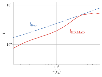
Figure 1: Non-relativistic Keplerian specific angular momentum (blue; $l_{\rm Kep}=r^{1/2}$) and MAD (red) normalized angular momentum flux vs. radius for $a=0.9$. The angular momentum in the hydrodynamic flow in the MAD, $l_{\rm HD,MAD}$, is sub-Keplerian as the gas falls onto the BH, indicating that some mechanism is robbing the disk of angular momentum thereby depriving the BH of the angular momentum supply.

3.1 BH spin evolution for NT and MAD flows

To determine BH spin evolution, we solved the coupled ODEs, equations (1), (2), and (3), for BH spin $a(m)$ and mass $M(m)$, for both the standard NT disk and MAD flows. Figure 2 shows the BH spin evolution $a(m)$ for the NT (Fig. 2a) and MAD (Fig. 2b) cases. The NT evolution is calculated using the equations described in Section 2.1. From each MAD simulation, we calculate the fluxes at the horizon, $e_{\rm in}$ and $l_{\rm in}$. We then interpolate these values over the full range of spins, generating the interpolation functions, $e_{\rm in}(a)$ and $l_{\rm in}(M,a)$, that we plug into the ODEs. We then solve the equations to model the full spin evolution.

For each disk type, we consider three values for the initial spin: $a_{0}=-1$, $a_{0}=0$, and $a_{0}=1$. For any initial spin $a_{0}$, the NT disk in Figure 2(a) will spin up the BH to equilibrium at the maximum $a_{\rm eq}=1$ before the BH has accreted twice its initial mass, $m/M_{0}=2$. The infalling gas supplies angular momentum and energy to the BH, and in the NT model there is nothing to remove angular momentum or energy from the BH. Thus, $a$ can only increase. For the MAD case shown in Figure 2(b), the BH spins down rapidly to the low value of $a_{\rm eq,MAD}\approx 0.07$, and in doing so it has only accreted roughly $50\%$ of its initial mass.

We illustrate how this timescale translates into physical units at the upper $x$-axis in Fig. 2 by adopting a fixed Eddington ratio, $\lambda_{0}$, and giving a cosmological spin-down timescale in Myrs. The Eddington accretion rate is given by $\dot{M}_{\rm Edd}=(4\pi Gm_{p}M)/(\epsilon\sigma_{\rm T}c)$, where $\sigma_{\rm T}$ is the Thomson cross-section. We assume a radiative efficiency, $\epsilon=0.1$. For a BH accreting at the Eddington rate ($\lambda_{0}=1$), the MAD BH will spin down to $a_{\rm eq}$ in approximately $22$ Myrs.

In order to explain how the equilibrium spin in the MAD case, $a_{\rm eq,MAD}$, can become so small, as well as why the spin-down is so much faster compared to the NT case, we need to understand the physics of the torques acting on the BH. First, we know that MADs launch powerful electromagnetic jets, and from the BZ model we know that they are powered by BH spin. Additionally, the accretion disk will exert a torque on the BH. Each in part carry their own angular momentum and energy. We now identify the influence of each of these factors.

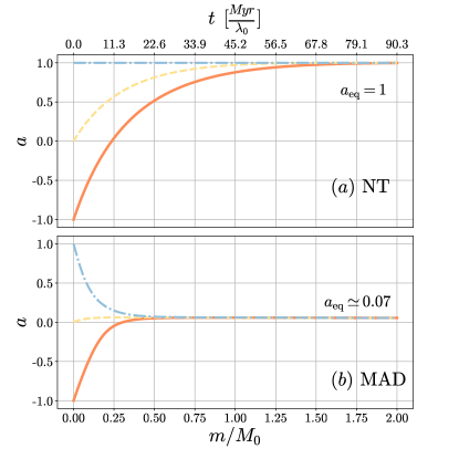
Figure 2: Dimensionless spin $a(m)$ and $a(t)$ for different values of initial spin: $a_{0}=-1$, $0$, $1$. The lower $x$-axis gives the mass accreted over the initial BH mass: when $m/M_{0}=1$, the BH has accreted its entire initial mass. The upper $x$-axis gives spin evolution in Myrs over an initial Eddington rate $\lambda_{0}$. [panel (a):] The BH with a Novikov-Thorne (NT) disk gains angular momentum and energy, and will spin up to $a_{\rm eq}=1$. [panel (b):] A MAD will spin down the BH to $a_{\rm eq}\approx 0.07$. The MAD spin-down timescale is very short (much shorter than NT spin-up timescale): the BH reaches its equilibrium spin after accreting only half of its initial mass. For a fixed $\lambda_{0}$, this spin-down timescale is independent of initial BH mass.

3.2 BH power output

We showed that in the NT disk, the BH can only spin up with time. The BH eats energy and angular momentum, and there are no large-scale magnetic fields to efficiently carry away the angular momentum. In a MAD, energy and angular momentum do not travel just into the horizon, but also outward in the form of jets and winds. They derive their power in part from the EM BZ power of the rapidly spinning BH. We define the EM power efficiency as the ratio of the time-averaged EM energy flux leaving the BH to the time-averaged rest mass flux entering the BH:

$$\eta_{\rm EM}=\frac{\langle P_{\rm EM}\rangle}{\langle\dot{m}\rangle c^{2}}.$$ (13)

We plot the EM efficiency $\eta_{\rm EM}$ as a function of spin in Figure 3. The electromagnetic energy flux on the BH is used to calculate the jet efficiency for each simulation and is shown as black points. To produce the pink and orange curves, we use the least squares fits in the form $C_{1}a^{4}+C_{2}a^{2}$ for each of the negative and positive values of $a$. This results in the fit for $\eta_{\rm EM}$:

$$\eta_{\rm EM}\times 100=\left\{\begin{array}[]{ll}-19.8a^{4}+48.9a^{2},&a\leq 0,\\ 106.3a^{4}+39.5a^{2},&a\geq 0.\\ \end{array}\right.$$ (14)

For a NT disk, $\eta_{\rm NT}$ never exceeds $45\%$. In the work of Gammie et al. (2004), the torque on the central BH was provided by a disk model that reached a maximum jet efficiency of $16\%$. MADs are known to achieve enormous efficiencies of $150\%$ (Tchekhovskoy et al., 2011) and even higher (McKinney et al., 2012). An efficiency of $100\%$ means that all accretion power is processed into jet power. Thus an efficiency exceeding $100\%$ implies that the jets are feeding on the angular momentum of the BH.

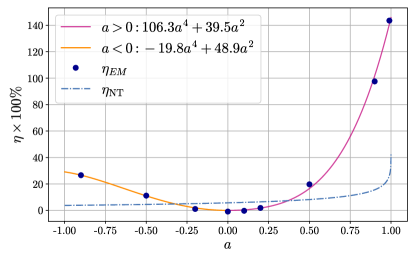
Figure 3: Dimensionless efficiency $\eta$ as a function of BH spin $a$ for different models. The radiative efficiency $\eta_{\rm NT}$ for the Novikov-Thorne disk is shown in the blue dash-dotted line, and the electromagnetic outflow efficiency $\eta_{\rm EM}=P_{\rm EM}/\dot{m}c^{2}$ at the event horizon is shown with dark blue dots. We provide separate fits to $\eta_{\rm EM}(a)$ dependence for positive (pink) and negative (orange) spins (see eq. 14). A rapidly-spinning BH fed by a MAD can achieve EM energy outflow efficiencies $>100\%$. These fits form the inputs to our semi-analytic MAD spin-down model.

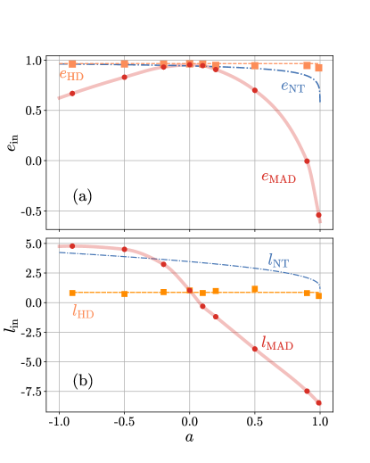
Figure 4: Specific energy and angular momentum fluxes in the Novikov-Thorne and MAD models. [panel (a):] Specific energy flux: The Novikov-Thorne energy flux, $e_{\rm NT}$, on the BH remains positive and decreases rapidly at high prograde spin (blue dash-dotted curve). In a MAD, the hydrodynamic portion, $e_{\rm HD}$, stays close to unity (orange dashed line), although it shows a slight decrease near $a=1$ (orange squares). Additionally accounting for the EM contribution leads to the total specific MAD energy flux, $e_{\rm MAD}$ (red dots connected by light red line). [panel (b):] In the NT model, the specific angular momentum flux, $l_{\rm in,NT}$, decreases with increasing spin (blue dash-dotted line). Surprisingly, in a MAD, $l_{\rm in,HD}$ is much smaller than the NT value (orange squares) and roughly constant at all spins: the MAD specific angular momentum flux is significantly sub-NT. In fact, the hydrodynamic component of the angular momentum flux is essentially constant across all values of spin (orange dashed line). In our semi-analytic model of MAD spin-down, we use the two (constant) fits shown with the dashed orange lines, $l_{\rm HD}$ and $e_{\rm HD}$.

For the BH to launch jets, it needs to hold magnetic flux. Jet power is directly proportional to magnetic flux, $\Phi_{\rm BH}$. BH generates jet power via the BZ mechanism at the efficiency (Blandford & Znajek, 1977; Tchekhovskoy, 2015),

$$\eta_{\rm BZ}=\frac{\langle P_{\rm BZ}\rangle}{\langle\dot{m}\rangle c^{2}}=\frac{\kappa}{4\pi c}\left(\frac{\Omega_{\rm H}r_{g}}{c}\right)^{2}\langle\phi^{2}_{\rm BH}\rangle f(\Omega_{\rm H}),$$ (15)

where $\kappa$ is a constant that depends on the magnetic field geometry (0.044 for a parabolic geometry), $\Omega_{\rm H}=ac/(2r_{\rm H})$ is the angular frequency of the BH horizon, $r_{\rm H}$ is the radius of the BH horizon, and $\Phi_{\rm BH}$ is the magnetic flux on the BH. The approximation, $f(\Omega_{\rm H})=1$, can be used for $a\leq 0.95$, but for rapidly-spinning BHs with $a>0.95$, the following approximation maintains accuracy, $f(\Omega_{\rm H})\approx 1+1.38(\Omega_{\rm H}r_{\rm g}/c)^{2}-9.2(\Omega_{\rm H}r_{\rm g}/c)^{4}$ (Tchekhovskoy, 2015). We use $\eta_{\rm BZ}$ to guide our choice of fit for $\eta_{\rm EM}$ in Figure 3 and equation (14).

3.3 Disk and jet contributions to spin-down

Both the disk and the jets exert a torque on the BH. To understand why the MAD spins down to such a low value of spin and why it happens so quickly, we now decompose the total torque into its EM and hydrodynamic constituents, which we compute via the corresponding fluxes at the event horizon. We distinguish the jets from the disk using a cutoff condition on the magnetization, $\sigma\equiv 2p_{\rm mag}/\rho c^{2}>30$; in the simulations, we set the density floor, which limits the magnetization to $\max\sigma=50$. Here, $p_{\rm mag}$ is the magnetic pressure. Using the above condition, we find that, unsurprisingly, most of the electromagnetic (EM) flux escapes through the jets, and most of the hydrodynamic flux enters through the disk. To keep things simple, from now on, we will assign the torque by the jets to be the entire electromagnetic component and the torque by the disk to be the entire hydrodynamic component. We note that despite this naming convention, some “jet” magnetic field lines may connect to the BH through the disk.

We plot specific angular momentum and energy fluxes vs. spin in Figure 4. Figure 4(a) shows that the NT disk (blue dashed line) supplies the BH the most angular momentum flux and energy flux at $a=-1$ and the least at $a=1$, and always supplies positive energy and angular momentum. The total MAD energy flux computed from our simulations, $e_{\rm MAD}$, is shown in red, where each data point corresponds to a simulation. We find that its hydrodynamic constituent remains roughly constant, $e_{\rm in,HD}\approx 0.97$, for all but the highest positive values of $a$. However, at such high values of $a$, it is the EM component that dominates $e_{\rm MAD}$. Figure 4(b) reveals that the hydrodynamic specific angular momentum (orange) supplied by the MAD is significantly less than that supplied by the NT disk. It is striking that $l_{\rm in,HD}$ remains roughly constant at $\approx 0.86$ for all values of $a$.

Interestingly, the MAD spin-down cannot be reproduced by simply taking the torque from the NT disk and adding the spin-down contribution from the jets. In fact, we cannot assume that the two disks supply the same angular momentum and energy to the BH. In fact, the MAD hydrodynamic torque is quite different than that of the NT disk. This is one reason for why the MAD spins the BHs down to $a_{\rm eq}\approx 0.07$, and why it happens so quickly: at every stage of its evolution, a MAD supplies very little angular momentum to the BH.

We illustrate the MAD spin-down in Figure 5 through the dimensionless spin-up parameter (Gammie et al., 2004), which is defined in equation (4). Whenever $s=0$ the BH spin is no longer evolving and has reached equilibrium. The blue dashed line shows the spin-up parameter for the thin Novikov-Thorne disk, where the blue vertical band shows where $s_{\rm NT}=0$ at $a=1$, just as we showed in Figure 2. The red curve shows the total spin-up from the MAD simulations and was calculated using the form of equation (5) with equations (10) and (11). The red vertical band shows $s_{\rm MAD}=0$ at $a\approx 0.1$, just as we showed $a_{\rm eq,MAD}\approx 0.1$ in Section 3.1. The spin-up parameter remains positive for a NT disk, since accretion supplies angular momentum and energy, increasing the BH spin. For a MAD with $s<0$, the BH loses energy to relativistic jets and its spin decreases back down to the equilibrium value.

We note that several simulations, e.g. those with $a=0.2$ and $a=0.5$, have a relatively short duration, which limits the time interval over which we averaged them over to measure the spin-up parameter (Table 1). However, the simulations that bracket the equilibrium spin, those for $a=0.0$ and $a=0.1$, extend out to later times. To compute the equilibrium spin numerically, we use linear interpolation between the simulated values of $s$ for these two longer simulations.

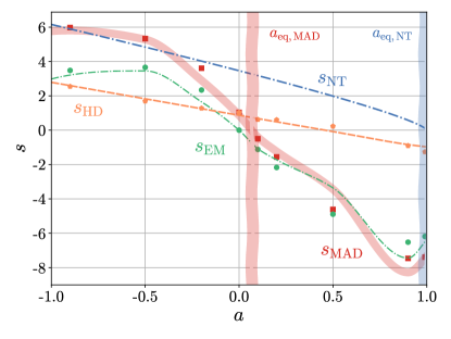
Figure 5: Dimensionless spin-up parameter $s$ as a function of BH spin $a$ for MAD and NT disk models. We show the NT model in blue. MAD hydrodynamic disk is shown in orange, and our model for the disk is shown by the dashed orange line. In a MAD, the disk component follows a similar trend as the NT disk, but its torque on the BH is much smaller except at the highest spin values. The EM component is shown in green, with our jet model shown by the green dashed line. The total MAD data is shown by red points, and our total MAD spin-down model is shown by the thick, red curve. The values of equilibrium spin $a_{\rm eq}$ for MAD and NT disks are shown as vertical lines at $a=0.1$ and $a=1$, respectively: these are where the spin-up curves vanish, $s=0$. Our semi-analytic $s_{\rm MAD}$ model agrees well with the simulation data. Differences for positive spin are primarily caused by an imperfect fit for $\eta_{\rm EM}$ (as seen in Fig. 3), affecting $s_{\rm EM}$. Our semi-analytic model for MAD torques on the BH shows how and why MADs spins down their BHs to a very low value of $a_{\rm eq,MAD}\approx 0.07$. MADs are significantly modified by the large-scale, dynamically-important magnetic fields.

3.4 Model for MAD spin-down

Here we construct a model that reproduces the MAD simulation data. Jet power must play an important role in BH spin-down because the jets extract BH rotational energy at high spin. Moderski & Sikora (1996) described the spin evolution, including the effect of jet-like outflows, analytically by taking the BH spin evolution equations (Eqns. 1 and 3) and including the terms for jet power. We write them as

$$\frac{da}{dt}=\frac{\dot{m}}{M}\left(l_{\rm in,HD}-2ae_{\rm in,HD}\right)-\frac{P_{\rm EM}}{Mc^{2}}\left(\frac{1}{k\Omega_{\rm H}}-2a\right)$$ (16)

and

$$\frac{d\log M}{dt}=\frac{\dot{m}}{M}e_{\rm in,HD}-\frac{P_{\rm EM}}{Mc^{2}},$$ (17)

where $k=\Omega_{\rm F}/\Omega_{\rm H}$, the ratio of the angular frequency of the magnetic field lines to the angular frequency of the BH event horizon, $\Omega_{\rm H}$. The first terms now only describe the disk (hydrodynamic) contributions.

As we did for the NT disk and MAD, we similarly recast equation (16) in the form of equation (4) to now determine how the disk and jets contribute to BH spin-up. The new expression for $s$ is then

$$s=\left(l_{\rm in,HD}-2ae_{\rm in,HD}\right)-\eta_{\rm EM}\left(\frac{1}{k\Omega_{\rm H}}-2a\right).$$ (18)

We now use approximate fits for $k$, $\Omega_{\rm H}$, $\eta_{\rm EM}$, $l_{\rm in,HD}$, and $e_{\rm in,HD}$ (see Figs. 3, 4, and 6) to construct our semi-analytic model. Namely, we approximate $l_{\rm in,HD}$ with the constant value, $l_{\rm HD,avg}=0.86$, and $e_{\rm in,HD}$ with the average value of $0.97$, both shown by the dashed orange lines in Figure 4. We use the fit, $\eta_{\rm EM}$, in the form $\eta\propto C_{1}a^{4}+C_{2}a^{2}$ as we show in Figure 3 and equation (15).

The standard monopole BZ model has $k=1/2$, which gives the maximum EM efficiency. We calculate $k$ at the horizon and then average in $t$, $\theta$ and $\phi$. Figure 6 shows that for our semi-analytic model, we approximate this dependence with the average value, $k=0.23$, for $a<0$. For $a>0$, we find a good fit for $k$,

$$k=\left\{\begin{array}[]{ll}0.23,&a<0,\\ \min(0.1+0.5a,0.35),&a>0.\\ \end{array}\right.$$

Similar to Penna et al. (2013), $k$ is smaller than what is predicted by the standard BZ model.

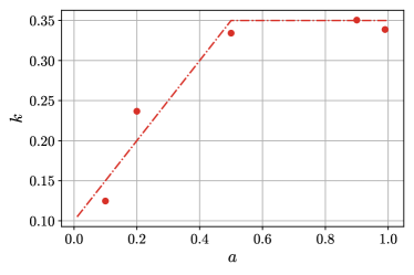
Figure 6: We plot $k=\Omega_{\rm F}/\Omega_{\rm H}$ and its dependence on spin, which is crucial for converting jet power into angular momentum in our semi-analytic model. The red dashed line shows the fit that we used to construct our analytic model for $a>0$. We did not find a strong dependence on spin for $a<0$ and so used a constant value, $k=0.23$, in our model for $a<0$.

For $a=0$, there is no energy extraction along the field lines because $\Omega_{\rm H}=0$, so we set the second term in equations (16), (17), and (18) to $0$. This might not be obvious in equations (16) and (18). However, because $\Omega_{\rm H}=ac/2r_{\rm H}$ and $\eta_{\rm EM}\propto a^{2}$, the $\Omega_{\rm H}\propto a$ term in the denominator cancels out: thus, for zero spin, this results in zero contribution from the jet terms (which contain $P_{\rm EM}$ and $\eta_{\rm EM}$).

With these constraints in our model we produce the thick red curve in Figure 5, which gives us the total MAD spin-up $s_{\rm MAD}$ curve. This fits the data well, and we expect that this analytic model to be useful for modeling spin evolution. See Section 4 for more details.

Figure 7 shows the spin, mass and jet efficiency evolution in MAD flows vs. time over a characteristic BH mass-doubling timescale $\tau$. The timescale $\tau$ is defined such that $t/\tau=m/M_{0}$, where $m$ is the accreted mass and $M_{0}$ is the initial BH mass. In the top panels of Fig. 7 we have fit the spin evolution to,

$$a(t)=|a_{0}-a_{\rm eq}|e^{-t/\tau_{\rm MAD}}+a_{\rm eq},$$ (19)

(black dotted line), where $\tau_{\rm MAD}=\tau/18.5$ and $a_{0}$ is the initial spin. The second row of panels from the top shows the dependence of BH mass $M$ vs. $t$, we find that both the total mass and irreducible mass of the BH eventually increase with time, as expected. Although the total and irreducible BH masses are initially distinct, they very soon converge, by $t/\tau\approx 0.05$. The bottom panel shows the efficiency $\eta$ vs. time. As the BH spins down, the EM efficiency drops. In comparison, the hydrodynamic efficiency, $|1-e_{in,\rm HD}|$, remains roughly constant, consistent with the fact that in MADs, the disk torques do not significantly affect BH spin evolution with time.

Interestingly, the inset in the left middle panel of Fig. 7 shows that for the prograde case, the total BH mass slightly decreases before increasing. We see that during the short time the BH mass decreases, the rapidly rotating BH is spinning down so fast that the total efficiency $\eta$, the red curve in the bottom panel of Fig. 7, exceeds $100\%$. This is the first demonstration that, as a function of time, the BH actually loses mass due to the jets outshining accretion. The cause of this phenomenon is that the BH rapidly loses rotation energy at high spin electromagnetically (through the jets), faster than the irreducible mass increases due to the energy supplied by accretion (through the disk).

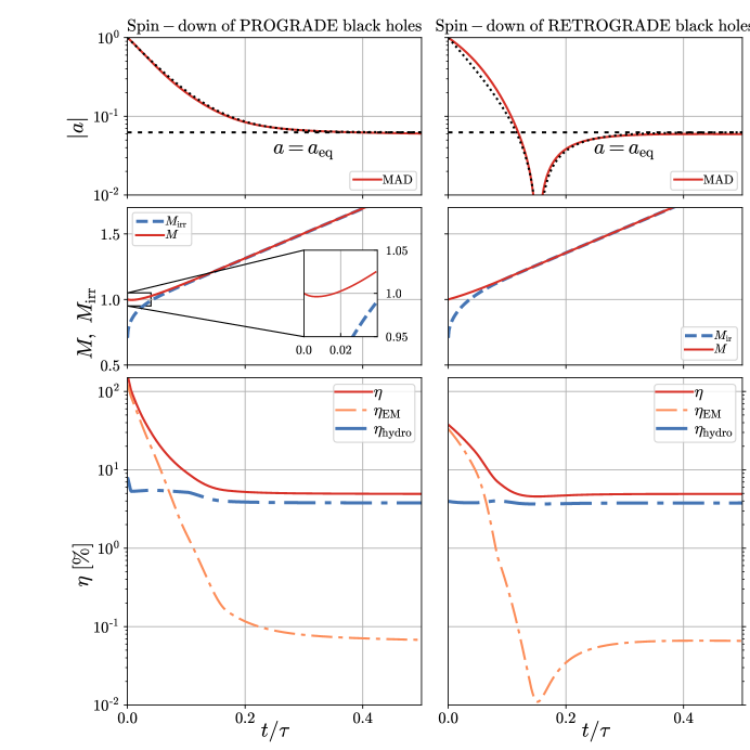
Figure 7: BH spin, mass, and efficiency vs. time for prograde (left column) and retrograde (right column) MADs; the time is measured in units of $\tau$, the timescale for the BH to accrete its own mass, $t/\tau=m/M_{0}$. [Top panel]: BH spin exponentially decays in time, closely following the fitting formula (19). A MAD BH will spin down to $a_{\rm eq}\approx 0.07$ by the time it has accreted a small fraction of its initial mass. For instance, a maximally spinning prograde BH spins down to $a=0.2$ by $t/\tau=0.1$, i.e., after consuming $10\%$ of its own mass, and to $a=0.1$ by $t/\tau=0.2$, i.e., after consuming $20\%$ of its own mass. [Middle panel]: Total BH mass (red solid) and irreducible BH mass (blue dashed) vs. time. At $t/\tau\lesssim 0.01$, the mass of the prograde BH briefly decreases before increasing again, as seen in the inset (left middle panel). This shows that BH loses rotational energy faster via the BZ mechanism than the accretion can replenish it (i.e., $\eta>100\%$). At later times, BH mass increases for both prograde and retrograde BHs. [Bottom panel]: Total (red), EM (orange), and hydrodynamic (blue) outflow energy efficiencies. In the prograde case, the EM efficiency drops by more than three orders of magnitude from $a=1$ to late times, when BH spin reaches its equilibrium value, $a_{\rm eq}\approx 0.07$.

3.5 Analytic model to calculate $a_{\rm eq}$ in MADs

Because the BH reaches $a_{\rm eq}$ when $s=0$, we can work backward and use our semi-analytic model to find the value of $a_{\rm eq}$ analytically. We set equation (18) to $0$ and solve for $a_{\rm eq}$. As before, we use the average values in our model for the disk fluxes: $\langle l_{in,\rm HD}\rangle\approx 0.87$ and $\langle e_{in,\rm HD}\rangle\approx 0.97$. We use the positive fit $\eta_{EM}\approx 0.4a^{2}$. For $k$ we use the fit for low positive spin, $k=0.1+0.5a$. For small $a$, $\Omega_{\rm H}\approx a/4$. Using these approximations, dropping any terms that are higher order than $\propto a^{2}$ (they are small for low spin), we get a quadratic equation for $a_{\rm eq}$ that gives us the positive solution, $a_{\rm eq,MAD}^{\rm analytic}\approx 0.06$. This is remarkably close to the equilibrium spin value we have obtained directly from the simulation results, $a_{\rm eq,MAD}^{\rm simulated}\approx 0.07$ (see Sec 3.1).

4 Discussion and Conclusion

4.1 Semi-analytic Model of MAD Spin-down

We have used a suite of 3D GRMHD simulations of MADs from Tchekhovskoy et al. (2011, 2012); Tchekhovskoy (2015) to study the BH spin evolution in MADs. Tchekhovskoy et al. (2012) were the first to find that a MAD will spin down a BH to an equilibrium spin of $a_{\rm eq}\approx 0.07$. Here, using the equations describing the BH spin evolution in time under the torques from the accretion disk and the jets, we showed that the MADs will cause the BH to rapidly spin down, such that the BH reaches its equilibrium spin after accreting only $50\%$ of its initial mass (see Fig. 2). Indeed, BH spin-down by a MAD disk is much more efficient than the BH spin-up by a NT disk (see Fig. 2).

Such a rapid spin-down might come as a surprise, because intuitively we think of accretion as spinning up the BH, by supplying it with the angular momentum. To understand the physics behind the MAD spin-down, we split up the torques acting on the BH into their hydrodynamic and magnetic components, as seen in Fig. 5. Figure 1 shows that some mechanism, likely magnetic fields threading the inner disk, robs the disk gas of its angular momentum before it can reach the BH: the MAD specific angular momentum lies below the Keplerian one and, in fact, it decreases towards the BH inside the innermost stable circular orbit (ISCO), inside of which the specific angular momentum is assumed to be constant in the NT model. We thus end up with a strongly sub-Keplerian disk whose specific angular momentum decreases even further inside the ISCO and hence carries into the BH very little angular momentum, which is available for spinning up the BH.

In addition to the magnetic fields extracting angular momentum from the BH’s gas supply, strong and dynamically-important magnetic fields, which thread the BH, extract the angular momentum from the BH and send it out to large distances in the form of jets. Thus, the low equilibrium BH spin is a consequence of both of these effects: the lower-than-expected angular momentum supplied by the disk gas pales in comparison with the large magnetically-mediated angular momentum extraction out of the BH by the large-scale magnetic flux (see Figs. 4 and 5).

To quantify this, we have developed the first semi-analytic model that quantitatively describes what causes the BHs in the radiatively-inefficient MAD state to spin down so efficiently. We find that the hydrodynamic angular momentum and energy fluxes are essentially independent of the BH spin, as seen in Fig. 4. Thus, to the accuracy we are interested in, the hydrodynamic angular momentum ($l_{\rm HD}$) and energy ($e_{\rm HD}$) flux values – which we take to be constants in our semi-analytic model – are unique properties of the MAD state, at least for the typical disk thickness that we have studied here ($h/r\approx 0.3$). Using equation (18), we now can compute the hydrodynamic contribution to the spin-up parameter, $s_{\rm HD}$, which we plot with the orange dashed line in Fig. 5. It is remarkable that the gas retains so little angular momentum by the time it reaches the BH: in fact, $s_{\rm HD}$ vanishes at $a=0.5$, which means that at $a>0.5$, the hydrodynamic torques spin down the BH. This means that if we were to consider a hypothetical hydrodynamic disk model with the structure identical to MAD (but without the magnetic fields), this model would result in $a_{\rm eq}\simeq 0.5$.

The final step in building our semi-analytic model is to account for the EM torques, which we do via including the energy and angular momentum EM fluxes: we compute the values of these fluxes using the fitting formulas for the spin-dependence of the jet efficiency ($\eta_{\rm EM}$, Fig. 3) and the angular velocity of the magnetic field lines ($k=\Omega_{\rm F}/\Omega_{\rm H}$, Fig. 6).

4.2 Whodunnit?

Equation 18 gives the sum of the hydrodynamic and EM contributions, thus completing our semi-analytic model and giving us the spin-up parameter, $s$, which is shown in Fig. 5 with the thick light red curve. The model is in good quantitative agreement with the numerical values for $s$, shown with dark red squares. This agreement is even more remarkable given that in order to keep the model as simple as possible, we purposefully used quite rough approximations for the free parameters in the model (e.g., $l_{\rm HD}$, $e_{\rm HD}$, and $k$), as we discussed in Sec. 4.1.

Figure 5 shows that MADs have $|s_{\rm EM}|\gg|s_{\rm hydro}|$, i.e., the EM torques dominate the hydrodynamic ones, over a wide range of spin, $a\gtrsim 0.2$. This is made uniquely possible by the strongly sub-NT angular momentum of MADs: the specific angular momentum of the MAD (orange dashed line) lies much lower than that of the NT disk (blue dash-dotted line).

To gauge the relative importance of the various process for the rapid BH spin-down in MADs, we consider hypothetical disk models that differ in crucial aspects from our MAD simulations. For instance, in order to quantify the importance of sub-Keplerian nature of MADs on the spin-down, let us consider a disk model whose EM structure is that of the MAD, but whose hydrodynamic structure is that of the NT model. This combination might provide a rough description of luminous MADs, whose disks are thinner and hence closer to NT. For such disks, the equilibrium spin would shift to higher $a$ values to satisfy $s_{\rm NT}+s_{\rm EM}=0$. From Fig. 5, we can approximately see that this happens at $a_{\rm eq}\approx 0.3$. This means that even if the accretion flow were Keplerian (instead of significantly sub-Keplerian), the jets would still be strong enough to spin down the BH to a rather low, albeit higher, spin. If, additionally, the EM outflow efficiency drops substantially in luminous MADs compared to non-radiative ones (e.g., $\eta_{\rm EM}$ in equation (18) is lower by a factor of 2 than in our simulations, similar to what is seen in radiation-transport simulations of luminous MADs at $L/L_{\rm Edd}=0.35$, Liska et al. 2022), then the spin would evolve to $s_{\rm NT}+0.5s_{\rm EM}=0$, resulting in the equilibrium spin of $a_{\rm eq}\lesssim 0.5$.

These observations can have interesting implications for luminous MADs, ones in which the large-scale magnetic flux is saturated on the BH, but those that can efficiently cool down to small values of scale height, $h/r\ll 1$. Such disks are particularly important because they can power luminous jetted quasars. The rotation profile of such thinner disks can be much closer to the Keplerian one than of our thick MADs. However, from the above arguments, it follows that even in this case the equilibrium spin can remain significantly below unity (e.g., $a_{\rm eq}\sim 0.2-0.5$), defying the standard expectation of the “standard” NT disk model.

4.3 Comparison to other works

There has been plentiful other theoretical work studying BH spin evolution. As we mentioned above, Bardeen (1970) was the first to compute an equilibrium spin for a BH surrounded by a turbulent disk, $a_{\rm eq}=1$. Fully turbulent relativistic disk solutions were also calculated by Popham & Gammie (1998). They obtained smaller equilibrium spins, as low as $a_{\rm eq}=0.8$. They achieved this by modifying the inner boundary condition for the angular momentum. They found that deviations from the Keplerian angular momentum profile controlled the equilibrium spin. Finally, the turbulent viscosity acting on the disk controls the angular momentum profile. We find striking similarities with our results as deviations from a Keplerian angular momentum profile are also important in our model.

Gammie et al. (2004) were the first to use simulations of magnetized disks to measure the spin-up parameter and try to determine the equilibrium spin. They computed a large equilibrium spin when compared to our simulations, $a_{\rm eq}\simeq 0.93$. A possible explanation for this discrepancy is that their simulations are only 2D. Furthermore, compared to MADs, the jet power they measure in their simulations is weak (McKinney & Gammie, 2004). In this work, we find that the magnetized jet is quintessential for the rapid BH spin-down. Thus, we expect the difference in the equilibrium spin to be primarily the consequence of the difference in the jet power.

Narayan et al. (2022) ran long-duration GRMHD simulations of MADs. They calculate the BH spin-up parameter as a function of BH spin. Using a fifth-degree polynomial fit for $a$, they measured an equilibrium spin of 0.04. This value is a factor of 2 smaller than ours. However, they only ran one simulation with a BH spin close to their $a_{\rm eq}$, which may limit the accuracy to which $a_{\rm eq}$ can be determined.

It is also possible that the spin-up parameter and the equilibrium spin weakly depend on time. Indeed, Narayan et al. (2022) ran their simulations for a much longer time than ours. We investigated this possibility by computing the spin-up parameter as a function of time in our simulations. We found that the spin-up parameter does not show obvious trends in time, at least for the duration of our simulations.

In comparison to our work, Narayan et al. (2022) focus on low-luminosity AGN and do not account for the change of BH mass when computing the time evolution of BH spin. This limits their ability to evolve the system to late times, when the BH spin approaches its equilibrium value.

4.4 Observational implications

Our 3D GRMHD simulations of radiatively-inefficient accretion flows may be best applied to the super-Eddington accretion regime: in this regime, the accretion flow is so dense and optically-thick that the radiation does not have the time to escape out of the accretion flow and is instead advected into the BH or ejected as part of the outflow.

Figure 7 shows the time evolution of the BH spin and the associated quantities over cosmological timescales. The bottom panels reveal that the spin-down leads to a considerable decrease in the jet efficiency, $P_{\rm jet}(a={1})/P_{\rm jet}(a=a_{\rm eq})>10^{3}$. This can have significant observational consequences.

In the context of AGN, this could naturally explain the reported $10^{3}$ spread in the radio loudness of AGN (Sikora et al., 2007). Indeed, radio-quiet quasars can have low spin, whereas radio-loud quasars can have high spin, as expected in the spin paradigm (Sec. 1). The typical challenge facing this paradigm is that in order to explain such a large spread requires radio-quiet AGN to have very small spin, much lower than expected in the chaotic accretion model (Volonteri et al., 2007; Tchekhovskoy et al., 2010). If AGN undergo spectral state transitions similar to microquasars, their central BHs would undergo periods of spin-down during the jetted MAD stages and spin-up during the jet-less stages. Thus, the radio-quiet AGN can form as the direct consequence of BH spin-down due to MADs.

Gravitational wave detections (Abbott et al., 2016, 2019a, 2021) have led to new ways of constraining BH spin. Indeed, the gravitational wave signals contain information on the angular momentum of the BHs and their binary. However, disentangling the BH spin distribution from this signal requires careful Bayesian analysis and is subject to multiple biases. García-Bellido et al. (2021) have performed such an analysis. They find that in all the configurations they consider for the BH spin directions, the BH spin distribution is centered around small spins ($a<0.2$). This result is consistent with prior LIGO/Virgo/KAGRA Collaboration results (Abbott et al., 2019b). This distribution is consistent with our measurement of the equilibrium spin.

We note that the mass distribution measured by the LIGO/Virgo/KAGRA collaboration leans toward intermediate-mass BHs (Abbott et al., 2019b). It is unclear if a super-Eddington accretion disk is present in the formation and evolution of intermediate-mass BHs. Indeed, other evolution pathways, like mergers, could lead to a BH spin distribution centered around small spins.

Gamma-ray bursts are some of the most powerful astrophysical phenomena in the universe. The collapsar model describes GRBs as the consequence of a failed supernova where all the energy of the gravitational collapse is funneled into a jet (Woosley, 1993). The jet is fed by the rotation of a central engine, a BH, through the BZ mechanism. Even though they are short events, lasting around 100 seconds, they are subject to very high accretion rates and are highly super-Eddington.

Recent large-scale GRMHD simulations of collapsars bridging the gap between the BH scales and the photosphere were run by Gottlieb et al. (2022a, b). They showed that their simulations achieve the MAD state and launch powerful jets. They also found that, for realistic conditions, the accretion rate can reach 0.01 solar masses per second. This accretion rate would lead to around 1 solar mass accreted for a GRB lasting around 100 seconds. For a BH of 2 solar masses, this would lead to a considerable spin-down (see Fig. 2). We should expect the remnant BHs to have a spin distribution centered around the equilibrium spin. The spin evolution during GRBs will be the subject of future work.

Furthermore, such a powerful spin-down could shut off the jet produced by the BH engine (see jet efficiency in Fig. 7, and recall that ${m}/{M_{0}}={t}/{\tau}$). If the jet power is reduced considerably, the weaker jet could have trouble escaping the stellar envelope. However, the engine activity may be controlled by the magnetic reservoir in the stellar envelope instead of the angular momentum reservoir in the central BH (Gottlieb et al., 2022a). Thus, our results imply that collapsar models need to take into account the effects of BH spin-down to model the evolution of the jet engine.

We do not expect the accretion disk to accrete at super-Eddington rates most of the time. Therefore, it is important to determine how radiative effects influence the spin evolution of BHs. Indeed, cooler disks will be thinner and will have different properties when compared to thicker super-Eddington disks: they tend to more closely resemble a Keplerian disk as the scale height decreases. Cooling will likely modify the angular momentum profile and possibly the jet structure. Therefore, a thinner MAD will have a different equilibrium spin. However, as described in Sec. 4.2, the equilibrium spin is still expected to be much lower than unity, even in the presence of radiative effects. Future work will focus on the effects of cooling on the spin evolution of MADs. This will provide insight into the physics and observational signatures of luminous quasars accreting at sub-Eddington rates, $1-10\%$ of $L_{\rm Edd}$.

References

- Abbott et al. (2016) Abbott, B. P., Abbott, R., Abbott, T. D., et al. 2016, Physical Review Letters, 116, 061102, doi: 10.1103/PhysRevLett.116.061102
- Abbott et al. (2019a) —. 2019a, Physical Review X, 9, 031040, doi: 10.1103/PhysRevX.9.031040
- Abbott et al. (2019b) —. 2019b, The Astrophysical Journal, 882, L24, doi: 10.3847/2041-8213/ab3800
- Abbott et al. (2021) Abbott, R., Abbott, T. D., Abraham, S., et al. 2021, Physical Review X, 11, 021053, doi: 10.1103/PhysRevX.11.021053
- Aird et al. (2018) Aird, J., Coil, A. L., & Georgakakis, A. 2018, MNRAS, 474, 1225, doi: 10.1093/mnras/stx2700
- Anglés-Alcázar et al. (2017) Anglés-Alcázar, D., Faucher-Giguère, C.-A., Quataert, E., et al. 2017, MNRAS, 472, L109, doi: 10.1093/mnrasl/slx161
- Balbus & Hawley (1991) Balbus, S. A., & Hawley, J. F. 1991, ApJ, 376, 214, doi: 10.1086/170270
- Balbus & Hawley (1998) Balbus, S. A., & Hawley, J. F. 1998, Rev. Mod. Phys., 70, 1, doi: 10.1103/RevModPhys.70.1
- Bardeen (1970) Bardeen, J. M. 1970, Nature, 226, 64, doi: 10.1038/226064a0
- Begelman & Volonteri (2017) Begelman, M. C., & Volonteri, M. 2017, MNRAS, 464, 1102, doi: 10.1093/mnras/stw2446
- Blandford (1999) Blandford, R. D. 1999, in Astronomical Society of the Pacific Conference Series, Vol. 160, Astrophysical Discs - an EC Summer School, ed. J. A. Sellwood & J. Goodman, 265
- Blandford & Rees (1992) Blandford, R. D., & Rees, M. J. 1992, in American Institute of Physics Conference Series, Vol. 254, Testing the AGN paradigm, ed. S. S. Holt, S. G. Neff, & C. M. Urry, 3–19
- Blandford & Znajek (1977) Blandford, R. D., & Znajek, R. L. 1977, MNRAS, 179, 433, doi: 10.1093/mnras/179.3.433
- Chen et al. (2021) Chen, Y., Gu, Q., Fan, J., et al. 2021, ApJ, 913, 93, doi: 10.3847/1538-4357/abf4ff
- Christie et al. (2019) Christie, I. M., Lalakos, A., Tchekhovskoy, A., et al. 2019, MNRAS, 490, 4811, doi: 10.1093/mnras/stz2552
- Ciotti & Ostriker (2007) Ciotti, L., & Ostriker, J. P. 2007, ApJ, 665, 1038, doi: 10.1086/519833
- Di Matteo et al. (2005) Di Matteo, T., Springel, V., & Hernquist, L. 2005, Nature, 433, 604, doi: 10.1038/nature03335
- Fender et al. (2010) Fender, R. P., Gallo, E., & Russell, D. 2010, MNRAS, 406, 1425, doi: 10.1111/j.1365-2966.2010.16754.x
- Ferrarese & Merritt (2000) Ferrarese, L., & Merritt, D. 2000, ApJ, 539, L9, doi: 10.1086/312838
- Fragile et al. (2012) Fragile, P. C., Gillespie, A., Monahan, T., Rodriguez, M., & Anninos, P. 2012, ApJS, 201, 9, doi: 10.1088/0067-0049/201/2/9
- Gammie et al. (2004) Gammie, C. F., Shapiro, S. L., & McKinney, J. C. 2004, ApJ, 602, 312, doi: 10.1086/380996
- García-Bellido et al. (2021) García-Bellido, J., Nuño Siles, J. F., & Ruiz Morales, E. 2021, Physics of the Dark Universe, 31, 100791, doi: 10.1016/j.dark.2021.100791
- Gitti et al. (2012) Gitti, M., Brighenti, F., & McNamara, B. R. 2012, Advances in Astronomy, 2012, 950641, doi: 10.1155/2012/950641
- Gottlieb et al. (2022a) Gottlieb, O., Lalakos, A., Bromberg, O., Liska, M., & Tchekhovskoy, A. 2022a, Monthly Notices of the Royal Astronomical Society, 510, 4962, doi: 10.1093/mnras/stab3784
- Gottlieb et al. (2022b) Gottlieb, O., Liska, M., Tchekhovskoy, A., et al. 2022b, The Astrophysical Journal, 933, L9, doi: 10.3847/2041-8213/ac7530
- Häring & Rix (2004) Häring, N., & Rix, H.-W. 2004, ApJ, 604, L89, doi: 10.1086/383567
- Izumi (2018) Izumi, T. 2018, PASJ, 70, L2, doi: 10.1093/pasj/psy045
- Jacquemin-Ide et al. (2021) Jacquemin-Ide, J., Lesur, G., & Ferreira, J. 2021, A&A, 647, A192, doi: 10.1051/0004-6361/202039322
- Jiang et al. (2019) Jiang, Y.-F., Stone, J. M., & Davis, S. W. 2019, ApJ, 880, 67, doi: 10.3847/1538-4357/ab29ff
- Jin et al. (2016) Jin, C., Done, C., & Ward, M. 2016, MNRAS, 455, 691, doi: 10.1093/mnras/stv2319
- Jin et al. (2017) —. 2017, MNRAS, 468, 3663, doi: 10.1093/mnras/stx718
- King (2003) King, A. 2003, ApJ, 596, L27, doi: 10.1086/379143
- King & Nealon (2021) King, A., & Nealon, R. 2021, MNRAS, 502, L1, doi: 10.1093/mnrasl/slaa200
- King (2010) King, A. R. 2010, MNRAS, 408, L95, doi: 10.1111/j.1745-3933.2010.00938.x
- Kitaki et al. (2017) Kitaki, T., Mineshige, S., Ohsuga, K., & Kawashima, T. 2017, PASJ, 69, 92, doi: 10.1093/pasj/psx101
- Komossa et al. (2006) Komossa, S., Voges, W., Xu, D., et al. 2006, AJ, 132, 531, doi: 10.1086/505043
- Kormendy & Ho (2013) Kormendy, J., & Ho, L. C. 2013, ARA&A, 51, 511, doi: 10.1146/annurev-astro-082708-101811
- Lanzuisi et al. (2016) Lanzuisi, G., Perna, M., Comastri, A., et al. 2016, A&A, 590, A77, doi: 10.1051/0004-6361/201628325
- Lasota et al. (2014) Lasota, J. P., Gourgoulhon, E., Abramowicz, M., Tchekhovskoy, A., & Narayan, R. 2014, Phys. Rev. D, 89, 024041, doi: 10.1103/PhysRevD.89.024041
- Liska et al. (2022) Liska, M. T. P., Musoke, G., Tchekhovskoy, A., Porth, O., & Beloborodov, A. M. 2022, ApJ, 935, L1, doi: 10.3847/2041-8213/ac84db
- MacDonald & Thorne (1982) MacDonald, D., & Thorne, K. S. 1982, MNRAS, 198, 345, doi: 10.1093/mnras/198.2.345
- Marconi & Hunt (2003) Marconi, A., & Hunt, L. K. 2003, ApJ, 589, L21, doi: 10.1086/375804
- Martínez-Sansigre & Rawlings (2011) Martínez-Sansigre, A., & Rawlings, S. 2011, MNRAS, 414, 1937, doi: 10.1111/j.1365-2966.2011.18512.x
- Mathur (2000) Mathur, S. 2000, MNRAS, 314, L17, doi: 10.1046/j.1365-8711.2000.03530.x
- McClintock et al. (2014) McClintock, J. E., Narayan, R., & Steiner, J. F. 2014, Space Sci. Rev., 183, 295, doi: 10.1007/s11214-013-0003-9
- McKinney & Gammie (2004) McKinney, J. C., & Gammie, C. F. 2004, The Astrophysical Journal, 611, 977, doi: 10.1086/422244
- McKinney et al. (2012) McKinney, J. C., Tchekhovskoy, A., & Blandford, R. D. 2012, MNRAS, 423, 3083, doi: 10.1111/j.1365-2966.2012.21074.x
- McNamara et al. (2009) McNamara, B. R., Kazemzadeh, F., Rafferty, D. A., et al. 2009, ApJ, 698, 594, doi: 10.1088/0004-637X/698/1/594
- Moderski & Sikora (1996) Moderski, R., & Sikora, M. 1996, MNRAS, 283, 854, doi: 10.1093/mnras/283.3.854
- Mortlock et al. (2011) Mortlock, D. J., Warren, S. J., Venemans, B. P., et al. 2011, Nature, 474, 616, doi: 10.1038/nature10159
- Narayan et al. (2022) Narayan, R., Chael, A., Chatterjee, K., Ricarte, A., & Curd, B. 2022, MNRAS, 511, 3795, doi: 10.1093/mnras/stac285
- Narayan & McClintock (2012) Narayan, R., & McClintock, J. E. 2012, MNRAS, 419, L69, doi: 10.1111/j.1745-3933.2011.01181.x
- Noble et al. (2009) Noble, S. C., Krolik, J. H., & Hawley, J. F. 2009, ApJ, 692, 411, doi: 10.1088/0004-637X/692/1/411
- Novikov & Thorne (1973) Novikov, I. D., & Thorne, K. S. 1973, in Black Holes (Les Astres Occlus), 343–450
- Paczynski & Xu (1994) Paczynski, B., & Xu, G. 1994, ApJ, 427, 708, doi: 10.1086/174178
- Penna et al. (2013) Penna, R. F., Narayan, R., & S\kadowski, A. 2013, MNRAS, 436, 3741, doi: 10.1093/mnras/stt1860
- Penrose (1969) Penrose, R. 1969, Nuovo Cimento Rivista Serie, 1, 252
- Popham & Gammie (1998) Popham, R., & Gammie, C. F. 1998, ApJ, 504, 419, doi: 10.1086/306054
- Pounds et al. (1995) Pounds, K. A., Done, C., & Osborne, J. P. 1995, MNRAS, 277, L5, doi: 10.1093/mnras/277.1.L5
- Rees (1988) Rees, M. J. 1988, Nature, 333, 523, doi: 10.1038/333523a0
- Reines & Volonteri (2015) Reines, A. E., & Volonteri, M. 2015, ApJ, 813, 82, doi: 10.1088/0004-637X/813/2/82
- Sanders & Fabian (2007) Sanders, J. S., & Fabian, A. C. 2007, Monthly Notices of the Royal Astronomical Society, 381, 1381–1399, doi: 10.1111/j.1365-2966.2007.12347.x
- Sikora et al. (2007) Sikora, M., Stawarz, Ł., & Lasota, J.-P. 2007, ApJ, 658, 815, doi: 10.1086/511972
- Silk & Rees (1998) Silk, J., & Rees, M. J. 1998, A&A, 331, L1. https://arxiv.org/abs/astro-ph/9801013
- S\kadowski et al. (2014) S\kadowski, A., Narayan, R., McKinney, J. C., & Tchekhovskoy, A. 2014, MNRAS, 439, 503, doi: 10.1093/mnras/stt2479
- Stanzione et al. (2020) Stanzione, D., West, J., Evans, R. T., et al. 2020, in Practice and Experience in Advanced Research Computing, 106–111
- Steiner et al. (2013) Steiner, J. F., McClintock, J. E., & Narayan, R. 2013, ApJ, 762, 104, doi: 10.1088/0004-637X/762/2/104
- Sutton et al. (2013) Sutton, A. D., Roberts, T. P., & Middleton, M. J. 2013, MNRAS, 435, 1758, doi: 10.1093/mnras/stt1419
- Szuszkiewicz (2004) Szuszkiewicz, E. 2004, in Coevolution of Black Holes and Galaxies, ed. L. C. Ho, 60
- Tchekhovskoy et al. (2012) Tchekhovskoy, A., McKinney, J. C., & Narayan, R. 2012, in Journal of Physics Conference Series, Vol. 372, Journal of Physics Conference Series, 012040
- Tchekhovskoy (2015) Tchekhovskoy, A. 2015, in Astrophysics and Space Science Library, Vol. 414, The Formation and Disruption of Black Hole Jets, ed. I. Contopoulos, D. Gabuzda, & N. Kylafis, 45
- Tchekhovskoy et al. (2010) Tchekhovskoy, A., Narayan, R., & McKinney, J. C. 2010, ApJ, 711, 50, doi: 10.1088/0004-637X/711/1/50
- Tchekhovskoy et al. (2011) —. 2011, MNRAS, 418, L79, doi: 10.1111/j.1745-3933.2011.01147.x
- Thorne (1974) Thorne, K. S. 1974, The Astrophysical Journal, 191, 507, doi: 10.1086/152991
- Thorne et al. (1990) Thorne, K. S., Price, R. H., MacDonald, D. A., & Fuchs, H. 1990, Astronomische Nachrichten, 311, 122
- Tsai et al. (2018) Tsai, C.-W., Eisenhardt, P. R. M., Jun, H. D., et al. 2018, ApJ, 868, 15, doi: 10.3847/1538-4357/aae698
- Volonteri & Rees (2005) Volonteri, M., & Rees, M. J. 2005, ApJ, 633, 624, doi: 10.1086/466521
- Volonteri et al. (2007) Volonteri, M., Sikora, M., & Lasota, J. 2007, The Astrophysical Journal, 667, 704–713, doi: 10.1086/521186
- Volonteri et al. (2015) Volonteri, M., Silk, J., & Dubus, G. 2015, ApJ, 804, 148, doi: 10.1088/0004-637X/804/2/148
- Walton et al. (2018) Walton, D. J., Fürst, F., Harrison, F. A., et al. 2018, MNRAS, 473, 4360, doi: 10.1093/mnras/stx2650
- Wilson & Colbert (1995) Wilson, A. S., & Colbert, E. J. M. 1995, ApJ, 438, 62, doi: 10.1086/175054
- Woosley (1993) Woosley, S. E. 1993, The Astrophysical Journal, 405, 273, doi: 10.1086/172359
- Wu et al. (2011) Wu, Q., Cao, X., & Wang, D.-X. 2011, ApJ, 735, 50, doi: 10.1088/0004-637X/735/1/50
- Yang et al. (2021) Yang, J., Wang, F., Fan, X., et al. 2021, ApJ, 923, 262, doi: 10.3847/1538-4357/ac2b32
- Yoo & Miralda-Escudé (2004) Yoo, J., & Miralda-Escudé, J. 2004, ApJ, 614, L25, doi: 10.1086/425416
- Zhuravleva et al. (2014) Zhuravleva, I., Churazov, E., Schekochihin, A. A., et al. 2014, Nature, 515, 85, doi: 10.1038/nature13830