Role of Bootstrap Averaging in Generalized Approximate Message Passing

Abstract

Generalized approximate message passing (GAMP) is a computationally efficient algorithm for estimating an unknown signal $\mathbf{\boldsymbol{w}}_{0}\in\mathbb{R}^{N}$ from a random linear measurement $\mathbf{\boldsymbol{y}}=X\mathbf{\boldsymbol{w}}_{0}+\mathbf{\boldsymbol{\epsilon}}\in\mathbb{R}^{M}$, where $X\in\mathbb{R}^{M\times N}$ is a known measurement matrix and $\mathbf{\boldsymbol{\epsilon}}$ is the noise vector. The salient feature of GAMP is that it can provide an unbiased estimator $\hat{\mathbf{\boldsymbol{r}}}^{\rm G}\sim\mathcal{N}(\mathbf{\boldsymbol{w}}_{0},\hat{s}^{2}I_{N})$, which can be used for various hypothesis-testing methods. In this study, we consider the bootstrap average of an unbiased estimator of GAMP for the elastic net. By numerically analyzing the state evolution of approximate message passing with resampling, which has been proposed for computing bootstrap statistics of the elastic net estimator, we investigate when the bootstrap averaging reduces the variance of the unbiased estimator and the effect of optimizing the size of each bootstrap sample and hyperparameter of the elastic net regularization in the asymptotic setting $M,N\to\infty,M/N\to\alpha\in(0,\infty)$. The results indicate that bootstrap averaging effectively reduces the variance of the unbiased estimator when the actual data generation process is inconsistent with the sparsity assumption of the regularization and the sample size is small. Furthermore, we find that when $\mathbf{\boldsymbol{w}}_{0}$ is less sparse, and the data size is small, the system undergoes a phase transition. The phase transition indicates the existence of the region where the ensemble average of unbiased estimators of GAMP for the elastic net norm minimization problem yields the unbiased estimator with the minimum variance.

I Introduction

Consider estimating an unknown signal $\mathbf{\boldsymbol{w}}_{0}\in\mathbb{R}^{N}$ from a random linear measurement $\mathbf{\boldsymbol{y}}\in\mathbb{R}^{M}$ in the form,

$$\mathbf{\boldsymbol{y}}=X\mathbf{\boldsymbol{w}}_{0}+\mathbf{\boldsymbol{\epsilon}}.$$ (1)

In (1), $X\in\mathbb{R}^{M\times N}$ is a known measurement matrix whose elements are independent and identically distributed (i.i.d.) standard Gaussian variables, and $\mathbf{\boldsymbol{\epsilon}}\sim\mathcal{N}(\mathbf{\boldsymbol{0}},\Delta I_{M})$ is the measurement noise. We also assume that each element of the unknown signal $\mathbf{\boldsymbol{w}}_{0}$ is i.i.d., according to a distribution $q_{0}$.

Generalized approximate message passing (GAMP) [1, 2] is a computationally efficient algorithm for solving this problem. A striking feature of GAMP is its applicability to various hypothesis testing [3]. Specifically, GAMP can provide an unbiased estimator $\hat{\mathbf{\boldsymbol{r}}}^{\rm G}\sim\mathcal{N}(\mathbf{\boldsymbol{w}}_{0},\hat{s}^{2}I_{M})$ [2] in a high-dimensional asymptotic setting with $M,N\to\infty,M/N\to\alpha\in(0,\infty)$, where the variance $\hat{s}^{2}$ depends on the quality of the measurement $\mathbf{\boldsymbol{y}}$ and denoising function used in GAMP. This unbiased estimator has been used to test the significance of estimated signals [4, 5, 3, 6].

The statistical power of these tests depends on the variance $\hat{s}^{2}$, with a lower variance leading to a higher statistical power. However, reducing the variance $\hat{s}^{2}$ is not a trivial task. Replacing the denoising function used in GAMP with a powerful one based on nonconvex regularization, for example, can worsen the convergence of GAMP [7] or, even if convergence is achieved, the improvement may be insignificant [8]. This study aims to find an alternative way to reduce the variance without nonconvex regularization.

To reduce the variance, we use the bootstrap averaging [9] of computational statistics (commonly known as ensemble learning in machine learning [10, 11]). Specifically, we consider averaging the unbiased estimators of GAMP for multiple bootstrap samples with arbitrary size $M\mu_{B},\,\mu_{B}\in(0,\infty]$. For denoising function of GAMP, we consider the one for the elastic net [12].

However, the efficient computation and theoretical analysis of an averaged unbiased estimator remains unresolved. To resolve this problem, we use AMP with resampling (AMPR) [13, 14] that has been proposed for computing bootstrap statistics of the elastic net estimator by running a variant of GAMP once. We will argue that AMPR is actually computing the bootstrap average of the unbiased estimators of GAMP. That is, the averaged unbiased estimator can be computed efficiently, and its variance can be analyzed using the state evolution (SE) of AMPR, which has been developed to analyze the performance of AMPR in [14, 13]. We then conduct a thorough numerical analysis of the SE of the AMPR to investigate when bootstrap averaging reduces the variance of the unbiased estimator, and what phenomena occur when optimizing the bootstrap sample size and the hyperparameter of the elastic net regularization.

The findings of this study are summarized as follows:

• As mentioned above, the averaged unbiased estimator is obtained by AMPR. Furthermore, its variance can be estimated using the output of AMPR without knowing the actual signal $\mathbf{\boldsymbol{w}}_{0}$. Thus, we can minimize the variance by adjusting the bootstrap sample size and the hyperparameters of the elastic net (see Section III and IV)

• The variance of the averaged unbiased estimator can be reduced via bootstrapping, especially when the true data generation process is inconsistent with the sparsity assumption of the regularization and the data size is insufficient (see Section V-B)

• When $\mathbf{\boldsymbol{w}}_{0}$ is less sparse, and the data size is small, a phase transition occurs. This phase transition indicates the existence of the region where the value of the regularization parameter is infinitesimally small, and the number of unique data points in each bootstrap sample is less than the dimension of $\mathbf{\boldsymbol{w}}_{0}$. That is, in this region, the ensemble average of the unbiased estimators of GAMP for the elastic norm minimization problem (also known as the minimum norm interpolation in machine learning [15, 16, 17]) yields the best averaged unbiased estimator (see Section V-C)

I-A Notation

$\mathcal{N}(\mu,\sigma^{2})$ denotes a Gaussian distribution with mean $\mu$ and variance $\sigma^{2}$ and ${\rm Poisson}(\mu_{B})$ denotes a Poisson distribution with mean $\mu_{B}$. For a random variable $X\sim p_{X}$, we denote by $\mathbb{E}_{X}[\dots]$ an average $\int(\dots)p_{X}(x)dx$. Given a vector $\mathbf{\boldsymbol{x}}\in\mathbb{R}^{N}$ and scalar function $f:\mathbb{R}\to\mathbb{R}$, we write $f(\mathbf{\boldsymbol{x}})$ for the vector obtained by applying $f$ componentwise. For a vector $\mathbf{\boldsymbol{x}}=(x_{1},x_{2},\dots,x_{N})^{\top}\in\mathbb{R}^{N}$, we denote by $\mathbf{\boldsymbol{x}}^{2}=(x_{1}^{2},x_{2}^{2},\dots,x_{N}^{2})^{\top}$ the componentwise operations and by $\langle\mathbf{\boldsymbol{x}}\rangle=N^{-1}\sum_{i=1}^{N}x_{i}$ the empirical average.

II Background on AMPR

Algorithm 1 AMPR

1:Measurement matrix $X\in\mathbb{R}^{M\times N}$, measurement $\mathbf{\boldsymbol{y}}\in\mathbb{R}^{M}$, denoising function $g$ and its derivative $g^{\prime}$ from (4) and (7), the bootstrap sample size $\mu_{B}\in(0,\infty]$, and the number of iterations $T_{\rm it}$.

2:Select initial $\mathbf{\boldsymbol{h}}_{0}\in\mathbb{R}^{N},\hat{Q}_{0},\hat{v}_{0}\in(0,\infty)$.

3:Set $\mathbf{\boldsymbol{z}}_{0}=\mathbf{\boldsymbol{0}}_{M},\alpha_{N}=M/N$.

4:Let $\mathbf{\boldsymbol{\xi}}$ and $c$ be random variables distributed as $\mathbf{\boldsymbol{\eta}}\sim\mathcal{N}(0,I_{N})$ and $c\sim{\rm Poisson}(\mu_{B})$.

5:for $t=0,1,\dots,T_{\rm it}-1$ do

6:     $\hat{\mathbf{\boldsymbol{w}}}_{t}=\mathbb{E}_{\mathbf{\boldsymbol{\eta}}}[g(\mathbf{\boldsymbol{h}}_{t}+\sqrt{\hat{v}_{t}}\mathbf{\boldsymbol{\eta}},\hat{Q}_{t})]$.

7:     $\chi_{t}=\langle\mathbb{E}_{\mathbf{\boldsymbol{\eta}}}[g^{\prime}(\mathbf{\boldsymbol{h}}_{t}+\sqrt{\hat{v}_{t}}\mathbf{\boldsymbol{\eta}},\hat{Q}_{t})]\rangle$.

8:     $v_{t}=\langle\mathbb{E}_{\mathbf{\boldsymbol{\eta}}}[g(\mathbf{\boldsymbol{h}}_{t}+\sqrt{\hat{v}_{t}}\mathbf{\boldsymbol{\eta}},\hat{Q}_{t})^{2}]-\hat{\mathbf{\boldsymbol{w}}}_{t}^{2}\rangle$.

9:     $f^{(1)}_{t+1}=\mathbb{E}_{c}[\frac{c/\mu_{B}}{1+c/\mu_{B}\chi_{t}}],\,f^{(2)}_{t+1}=\mathbb{E}_{c}[(\frac{c/\mu_{B}}{1+c/\mu_{B}\chi_{t}})^{2}]$.

10:     $\hat{Q}_{t+1}=\alpha_{N}f^{(1)}_{t+1}$.

11:     $\mathbf{\boldsymbol{a}}_{t+1}=f_{t+1}^{(1)}(\mathbf{\boldsymbol{y}}-X\hat{\mathbf{\boldsymbol{w}}_{t}}+\chi_{t}\mathbf{\boldsymbol{a}}_{t})$.

12:     $\mathbf{\boldsymbol{h}}_{t+1}=X^{\top}\mathbf{\boldsymbol{a}}_{t}+\hat{Q}_{t+1}\hat{\mathbf{\boldsymbol{w}}}_{t}$.

13:     $\hat{v}_{t+1}=\alpha_{N}(f_{t+1}^{(2)}v_{t}+\frac{f_{t+1}^{(2)}-(f_{t+1}^{(1)})^{2}}{(f_{t+1}^{(t)})^{2}}\langle\mathbf{\boldsymbol{a}}_{t+1}^{2}\rangle)$ .

14:end for

15:Return $(\mathbf{\boldsymbol{h}}_{T_{\rm it}},\hat{Q}_{T_{\rm it}},\hat{v}_{T_{\rm it}})$.

II-A AMPR

Algorithm 1 shows AMPR [13] with an elastic net denoising function. Function $g:\mathbb{R}\times(0,\infty)\to\mathbb{R}$ is the elastic net denoising function and $g^{\prime}$ is a derivative of $g$ with respect to the first argument:

$$g(h,\hat{Q}) = \left\{\,\begin{IEEEeqnarraybox}[]{[}][c]{l?s}\IEEEstrut 0&if$|h| \leq\lambda\gamma$,\\ \frac{h-{\rm sgn}(h)\gamma\lambda}{\hat{Q}+\lambda(1-\gamma)}&otherwise,\IEEEstrut\end{IEEEeqnarraybox}\right.$$ (4)

$$g^{\prime}(h,\hat{Q}) = \left\{\,\begin{IEEEeqnarraybox}[]{[}][c]{l?s}\IEEEstrut 0&if$|h| \leq\lambda\gamma$,\\ \frac{1}{\hat{Q}+\lambda(1-\gamma)}&otherwise.\IEEEstrut\end{IEEEeqnarraybox}\right.$$ (7)

where $\lambda>0$ represents the regularization strength and $\gamma\in[0,1]$ is the $\ell_{1}$-ratio. At a fixed point, AMPR offers bootstrap statistics of the elastic net estimator as follows:

Proposition 1 (bootstrap statistics based on AMPR [13])

Let $\hat{\mathbf{\boldsymbol{w}}}^{\ast}$ be the elastic net estimator for a bootstrap sample $D^{\ast}$ of size $\mu_{B}M$.

$$\hat{\mathbf{\boldsymbol{w}}}^{\ast}=\mathop{\rm argmin}_{\mathbf{\boldsymbol{w}}\in\mathbb{R}^{N}}\sum_{\mu=1}^{M}\frac{c_{\mu}}{2\mu_{B}}(y_{\mu}-\mathbf{\boldsymbol{x}}_{\mu}^{\top}\mathbf{\boldsymbol{w}})^{2}+\sum_{i=1}^{N}\lambda(\gamma|w_{i}|+\frac{1-\gamma}{2}w_{i}^{2}),$$ (8)

where $c_{\mu}\sim_{\rm i.i.d.}{\rm Poisson}(\mu_{B})$ represents the number of times the data point $(\mathbf{\boldsymbol{x}}_{\mu},y_{\mu})$, $\mathbf{\boldsymbol{x}}_{\mu}$ being the $\mu$-th row of $X$, appears in the bootstrap sample $D^{\ast}$. Then once the AMPR reaches its fixed point at sufficiently large $T_{\rm it}$, the bootstrap statistics of $\hat{\mathbf{\boldsymbol{w}}}^{\ast}$ can be computed as

$$\mathbb{E}_{\mathbf{\boldsymbol{c}}}\left[\psi(\hat{w}_{i}^{\ast})\right]=\mathbb{E}_{\eta}[\psi(g(h_{i}+\sqrt{\hat{v}}\eta,\hat{Q}))],\quad\eta\sim\mathcal{N}(0,1),$$ (9)

where $\psi:\mathbb{R}\to\mathbb{R}$ is such that the expression in (9) is well-defined and otherwise arbitrary. The variables without iteration indexes $(h_{i},\hat{v},\hat{Q})$ are the output of AMPR at a fixed point.

Note that the averages $\mathbb{E}_{\eta}[g(h+\sqrt{\hat{v}}\eta;\hat{Q})],\mathbb{E}_{\eta}[g(h+\sqrt{\hat{v}}\eta;\hat{Q})^{2}]$ and $\mathbb{E}_{\eta}[g^{\prime}(h+\sqrt{\hat{v}}\eta;\hat{Q})]$ can be written in closed-form by the error function, thus computing these quantities is computationally easy. Also, $\mathbb{E}_{c}[\dots]$ is an average over a one-dimensional discrete random variable. It can be computed numerically without much computational overhead. Hence the computational complexity of computing the RHS of (9) is dominated by the matrix-vector product operations in lines 11-12 of Algorithm 1 instead of repeatedly computing $\hat{\mathbf{\boldsymbol{w}}}^{\ast}$ for numerous realizations of $\mathbf{\boldsymbol{c}}$, making AMPR a computationally efficient algorithm for computing the bootstrap statistics.

II-B SE of AMPR

Algorithm 2 SE of AMPR

1:Initial state of AMPR $(\mathcal{E}_{0},\hat{Q}_{1},\hat{v}_{1})$, variance of the measurement noise $\Delta$, distribution $q_{0}$ of the signal $\mathbf{\boldsymbol{w}}_{0}$, measurement ratio $\alpha$, denoising function $g$ and its derivative $g^{\prime}$ from (4) and (7), the bootstrap sample size $\mu_{B}\in(0,\infty]$, and the number of iterations $T_{\rm it}$.

2:Set $\hat{\chi}_{1}=\alpha^{-1}\hat{Q}_{1}^{2}(\mathcal{E}_{0}+\Delta)$

3:Let $\xi,\eta,w_{0}$ and $c$ be random variables distributed as $\xi,\eta\sim\mathcal{N}(0,1),w_{0}\sim q_{0}$, and $c\sim{\rm Poisson}(\mu_{B})$.

4:for $t=1,\dots,T_{\rm it}-1$ do

5:     $\hat{w}_{t}=g(\hat{Q}_{t}w_{0}+\sqrt{\hat{\chi}_{t}}\xi+\sqrt{\hat{v}_{t}}\eta;\hat{Q}_{t})$.

6:     $\mathcal{E}_{t}=\mathbb{E}_{w_{0},\xi}[(\mathbb{E}_{\eta}[\hat{w}_{t}]-w_{0})^{2}]$

7:     $\chi_{t}=\mathbb{E}_{w_{0},\xi,\eta}[g^{\prime}(\hat{Q}_{t}w_{0}+\sqrt{\hat{\chi}_{t}}\xi+\sqrt{\hat{v}_{t}}\eta,\hat{Q}_{t})]$.

8:     $v_{t}=\mathbb{E}_{w_{0},\xi}[\mathbb{E}_{\eta}[\hat{w}_{t}^{2}]-\mathbb{E}_{\eta}[\hat{w}_{t}]^{2}]$.

9:     $f^{(1)}_{t+1}=\mathbb{E}_{c}[\frac{c/\mu_{B}}{1+c/\mu_{B}\chi_{t}}],\,f^{(2)}_{t+1}=\mathbb{E}_{c}[(\frac{c/\mu_{B}}{1+c/\mu_{B}\chi_{t}})^{2}]$.

10:     $\hat{Q}_{t+1}=\alpha f^{(1)}_{t+1}$.

11:     $\hat{\chi}_{t+1}=\alpha(f_{t+1}^{(1)})^{2}(\mathcal{E}_{t}+\Delta)$

12:     $\hat{v}_{t+1}=\alpha(f_{t+1}^{(2)}v_{t}+(f_{t+1}^{(2)}-(f_{t+1}^{(1)})^{2})\mathcal{E}_{t})$ .

13:end for

AMPR displays remarkable behavior. Let $\hat{\mathbf{\boldsymbol{r}}}_{t}=\mathbf{\boldsymbol{h}}_{t}/\hat{Q}_{t},t=1,2,\dots,T_{\rm it}.$ Then $\hat{\mathbf{\boldsymbol{r}}}_{t}$ behaves like a white Gaussian noise-corrupted version of the true signal $\mathbf{\boldsymbol{w}}_{0}$ [13]. Furthermore, the variance can be estimated using SE.

Proposition 2 (SE of AMPR [13])

$\hat{\mathbf{\boldsymbol{r}}}_{t}$ behaves as a white Gaussian noise-corrupted version of the actual signal $\mathbf{\boldsymbol{w}}_{0}$:

$$\hat{\mathbf{\boldsymbol{r}}}_{t}\sim\mathcal{N}(\mathbf{\boldsymbol{w}}_{0},\hat{\sigma}_{t}^{2}),\quad\hat{\sigma}^{2}_{t}=\hat{\chi}_{t}/\hat{Q}_{t}^{2},$$ (10)

for some positive value $\hat{\chi}_{t}$, indicating that $\hat{\mathbf{\boldsymbol{r}}}_{t}$ can be used as an unbiased estimate of $\mathbf{\boldsymbol{w}}_{0}$. The variance is predicted in the asymptotic setting $M,N\to\infty,M/N\to\alpha\in(0,\infty)$ using the scalar SE specified in Algorithm 2. There, $\mathcal{E}_{t},t=1,2,\dots$ corresponds to the mean squared error (MSE) of the AMPR estimate $\hat{\mathbf{\boldsymbol{w}}}_{t}$: $\mathcal{E}_{t}=N^{-1}\|\hat{\mathbf{\boldsymbol{w}}}_{t}-\mathbf{\boldsymbol{w}}_{0}\|_{2}^{2}$. To track the performance of AMPR, $\mathcal{E}_{0}$ should be inputted as the MSE of $\hat{\mathbf{\boldsymbol{w}}}_{0}$.

Using the SE of the AMPR, we can predict the variance of the unbiased estimator in the asymptotic setting $M,N\to\infty,M/N\to\alpha\in(0,\infty)$ for each value of $\mu_{B},\lambda$, and $\gamma$. Hence variance can be minimized by tuning $(\mu_{B},\lambda,\gamma)$ using versatile black-box optimization methods implemented in various optimization libraries [18, 19].

III Averaged unbiased estimator

Here, we explain the meaning of the SE of AMPR. Subsequently, we argue that $\hat{\mathbf{\boldsymbol{r}}}_{t}$ of AMPR is the bootstrap average of the unbiased estimators of GAMP.

The first point is the meaning of $\xi$ and $\eta$ that appear in SE. Propositions 1 and 2 indicate that, once the AMPR reaches its fixed point at sufficiently large $T_{\rm it}$, for any functions $\phi,\psi:\mathbb{R}\to\mathbb{R}$ such that the following expression is well defined, the following holds in the asymptotic setting $M,N\to\infty,M/N\to\alpha\in(0,\infty)$:

$$\frac{1}{N}\sum_{i=1}^{N}\phi\left(\mathbb{E}_{\mathbf{\boldsymbol{c}}}[\psi(\hat{w}_{i}^{\ast})]\right)\to\mathbb{E}_{w_{0},\xi}\left[\phi\left(\mathbb{E}_{\eta}[\psi(g(\hat{Q}w_{0}\right.\right.\\ \left.\left.+\sqrt{\hat{\chi}}\xi+\sqrt{\hat{v}}\eta;\hat{Q}))]\right)\right],$$ (11)

where the variables $\hat{Q},\hat{\chi},\hat{v}$ are the outputs of SE at a fixed point. In (11), one can interpret that $\xi$ and $\eta$ effectively represents the randomness originating from $(X,\mathbf{\boldsymbol{y}})$ and $\mathbf{\boldsymbol{c}}$, respectively.

The next point is the relationship between AMPR and GAMP. For this, we define $\bar{q}_{t}\equiv\mathcal{E}_{t}+v_{t}$ and $\bar{\chi}_{t}=\hat{\chi}_{t}+\hat{v}_{t}$. Then, the evolution of $(\hat{Q}_{t},\bar{\chi}_{t},\bar{q}_{t},\chi_{t})$ is equivalent to the SE of GAMP for computing $\hat{\mathbf{\boldsymbol{w}}}^{\ast}$ for one realization of $\mathbf{\boldsymbol{c}}$ [1, 2]. Recall that $\hat{\mathbf{\boldsymbol{w}}}^{\ast}$ is specified in (8). In addition, $\bar{\chi}_{t}/\hat{Q}_{t}^{2}\,(=(\mathcal{E}_{t}+\hat{v}_{t})/\hat{Q}_{t}^{2})$ represents the variance of the unbiased estimate of GAMP $\hat{\mathbf{\boldsymbol{r}}}_{t}^{\rm G}(\mathbf{\boldsymbol{c}})$ at each iteration. These observations indicate that the unbiased estimator of GAMP at each iteration $t$ can be decomposed into two Gaussian variables:

$$\hat{\mathbf{\boldsymbol{r}}}_{t}^{\rm G}(\mathbf{\boldsymbol{c}}) = \mathbf{\boldsymbol{w}}_{0}+\frac{\sqrt{\bar{\chi}_{t}}}{\hat{Q}_{t}}\mathbf{\boldsymbol{\xi_{0}}}=\mathbf{\boldsymbol{w}}_{0}+\frac{\sqrt{\hat{\chi}_{t}}}{\hat{Q}_{t}}\mathbf{\boldsymbol{\xi}}+\frac{\sqrt{\hat{v}_{t}}}{\hat{Q}_{t}}\mathbf{\boldsymbol{\eta}},$$ (12)

where $\mathbf{\boldsymbol{\xi}}_{0},\mathbf{\boldsymbol{\xi}},\mathbf{\boldsymbol{\eta}}\sim\mathcal{N}(0,I_{N})$, and $\mathbf{\boldsymbol{\xi}}$ and $\mathbf{\boldsymbol{\eta}}$ represent the randomness originating from $(X,\mathbf{\boldsymbol{y}})$ and $\mathbf{\boldsymbol{c}}$, respectively. We can interpret that AMPR computes the bootstrap statistics by decomposing $\mathbf{\boldsymbol{\xi}}_{0}$ into $\mathbf{\boldsymbol{\xi}}$ and $\mathbf{\boldsymbol{\eta}}$, and averaging over $\mathbf{\boldsymbol{\eta}}$. This yields the unbiased estimator $\hat{\mathbf{\boldsymbol{r}}}_{t}$ as in (10) that is the bootstrap average of $\hat{\mathbf{\boldsymbol{r}}}^{\rm G}(\mathbf{\boldsymbol{cka}})$. We verify this point numerically in section V-A (see Fig. 1 and 2).

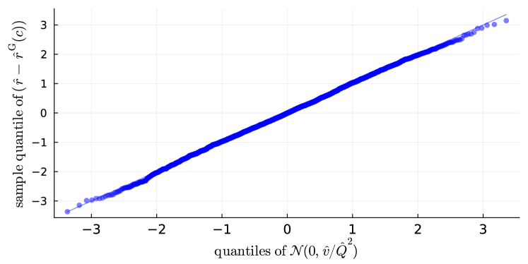
Figure 1: Q-Q plot of $\hat{\mathbf{\boldsymbol{r}}}-\hat{\mathbf{\boldsymbol{r}}}^{\rm G}(\mathbf{\boldsymbol{c}})$ for one realization of $X,\mathbf{\boldsymbol{y}}$, and $\mathbf{\boldsymbol{c}}$. The parameters are set as $(N,\alpha,\Delta,\lambda,\gamma,\mu_{B},\rho)=(4096,0.25,0.1,0.5,0.5,0.1)$.

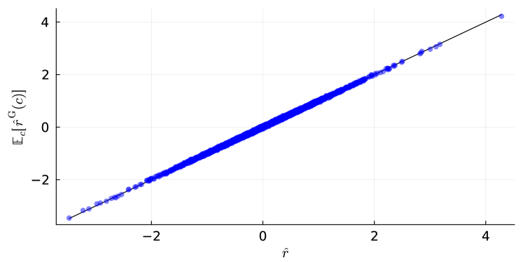
Figure 2: Scatter plot for $\hat{\mathbf{\boldsymbol{r}}}$ and $\mathbb{E}_{\mathbf{\boldsymbol{c}}}[\hat{\mathbf{\boldsymbol{r}}}^{\rm G}(\mathbf{\boldsymbol{c}})]$ for one realization of $X,\mathbf{\boldsymbol{y}}$. The parameters are set as $(N,\alpha,\Delta,\lambda,\gamma,\mu_{B},\rho)=(4096,0.8,0.25,0.1,0.5,0.5,0.1)$. $\mathbb{E}_{\mathbf{\boldsymbol{c}}}[\hat{\mathbf{\boldsymbol{r}}}^{\rm G}(\mathbf{\boldsymbol{c}})]$ was computed from $65536$ realizations of $\mathbf{\boldsymbol{c}}$.

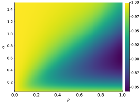
(a)

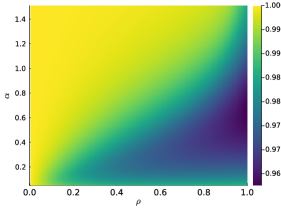
(b)

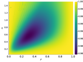
(c)

Figure 3: Ratio of optimal variances $\hat{\sigma}^{2}/\hat{s}^{2}$ is plotted against the sparsity of the true signal $\rho$ and the measurement ratio $\alpha$ as heat maps. In panels (a) and (b), the $\ell_{1}$-ratio of the elastic net regularization is fixed. In panel (c), the $\ell_{1}$-ratio is also optimized. The measurement noise is set as $\Delta=0.15$.

IV Variance optimization

In this section, we describe the properties of the variance of the unbiased estimate of AMPR.

First, the following proposition states that bootstrap averaging for the optimal choice of $(\mu_{B},\lambda,\gamma)$ does not increase the variance of the unbiased estimator.

Proposition 3

Let $\hat{s}^{2}$ be the variance of the unbiased estimator of GAMP at a fixed point to compute the elastic net estimator $\hat{\mathbf{\boldsymbol{w}}}$ of $D=(X,\mathbf{\boldsymbol{y}})$: $\hat{\mathbf{\boldsymbol{w}}}=\mathop{\rm argmin}_{\mathbf{\boldsymbol{w}}\in\mathbb{R}^{N}}\frac{1}{2}\sum_{\mu=1}^{M}(y_{\mu}-\mathbf{\boldsymbol{a}}_{\mu}^{\top}\mathbf{\boldsymbol{w}})^{2}+\sum_{i=1}^{N}\lambda(\gamma|w_{i}|+\frac{1-\gamma}{2})w_{i}^{2}$. We can select the parameter $(\mu_{B}^{\star},\lambda^{\star},\gamma^{\star})$ such that the variance of AMPR’s unbiased estimator $\hat{\sigma}^{2}$ at a fixed point does not exceed $\hat{s}^{2}$.

Proof:

We denote by $\hat{v},v$ the values of $\hat{v}_{t}$ and $v_{t}$ at the fixed point of the SE of AMPR. We consider the limit $\mu_{B}\to\infty$. In this limit, the random variable $c/\mu_{B},c\sim{\rm Poisson}(\mu_{B})$ that appears in (8) and Algorithm 1 behaves deterministically; the mean and variance of $c/\mu_{B}$ converge to $1$ and $0$. Then proposition 1 indicates that $\hat{v}=0$. Moreover, from line 12 in Algorithm 2, $\hat{v}=0$ implies $v=0$, which yields the GAMP algorithm for computing the elastic net estimator of $D$ [1]. ∎

Although SE prediction of the variance of $\hat{\mathbf{\boldsymbol{r}}}_{t}$ requires information on the unknown signal $\mathbf{\boldsymbol{w}}_{0}$, we can predict the variance from the data. In other words, estimating the variance of $\hat{\mathbf{\boldsymbol{r}}}_{t}$ does not require explicit knowledge on $\mathbf{\boldsymbol{w}}_{0}$.

Proposition 4 (Variance estimation from data)

In the asymptotic setting $M,N\to\infty,M/N\to\alpha\in(0,\infty)$, the variance $\hat{\sigma}_{t}^{2}$ of the unbiased estimate $\hat{\mathbf{\boldsymbol{r}}}_{t}$ can be estimated as

$$\hat{\sigma}_{t}^{2}=\alpha\langle\mathbf{\boldsymbol{a}}_{t}^{2}\rangle/\hat{Q}_{t}^{2}.$$ (13)

Proof:

In SE of AMPR, $\hat{\chi}_{t}/\hat{Q}_{t}^{2}$ is determined by the MSE $\mathcal{E}_{t-1}$ and variance of measurement noise $\Delta$ as $\hat{\chi}_{t}/\hat{Q}_{t}^{2}=\alpha^{-1}(\mathcal{E}_{t-1}+\Delta)$. For linear models, $\mathcal{E}_{t-1}+\Delta$ corresponds to the prediction error for a new sample and can be estimated using the leave-one-out error (LOOE) [20]. LOOE can be estimated from $\mathbf{\boldsymbol{a}}_{t}$ because it is proportional to the leave-one-out estimate for the data point $\mu$: $a_{t,\mu}=\hat{Q}_{t}\alpha^{-1}(y_{\mu}-\mathbf{\boldsymbol{x}}_{\mu}^{\top}\hat{\mathbf{\boldsymbol{w}}}_{t}^{\backslash\mu})$, where $\hat{\mathbf{\boldsymbol{w}}}_{t}^{\backslash\mu}$ is the AMPR’s estimate of $\mathbf{\boldsymbol{w}}_{0}$ without the sample $\mu$ (Equation (19) of reference [13]). ∎

Propositions 3 and 4 indicate that the variance $\hat{\sigma}^{2}$ can be minimized even if the signal $\mathbf{\boldsymbol{w}}_{0}$ is unknown. However, we use SE for the theoretical assessment in the next section for convenience.

V Numerical analysis

In the sequel, by numerically minimizing the variance using SE, we investigate when bootstrapping reduces the variance of the unbiased estimator and the phenomena that occur when optimizing the bootstrap sample size $\mu_{B}$ and the hyperparameter of the elastic net regularization $(\lambda,\gamma)$.

For this, we searched for the optimal parameter $(\mu_{B}^{\star},\lambda^{\star},\gamma^{\star})$ that yielded the minimum variance using the SE of AMPR and the Nelder-Mead algorithm in the Optim.jl library [18]. We obtained the fixed point of the SE by iterating the SE a sufficient number of times. For comparison, the same optimization was performed for the non-bootstrap case. For the signal distribution $q_{0}$, we consider the Gauss-Bernoulli model: $q_{0}=\rho\delta_{0}+(1-\rho)\mathcal{N}(0,1)$, with sparsity $\rho\in(0,1)$.

In this section, we denote the outputs of the AMPR or GAMP at fixed points by unindexed variables.

V-A Distribution of the unbiased estimator

We verified the interpretation of AMPR’s output $\hat{\mathbf{\boldsymbol{r}}}$ described in Section III. For this, we compared the output of GAMP $\hat{\mathbf{\boldsymbol{r}}}^{\rm G}(\mathbf{\boldsymbol{c}})$ for each realization of $\mathbf{\boldsymbol{c}}$ as in (8), and the output of AMPR. The parameters used to produce the figure were set as $(N,\alpha,\Delta,\lambda,\gamma,\mu_{B},\rho)=(4096,0.8,0.25,0.1,0.5,0.5,0.1)$.

Fig. 1 shows the sample quantiles of $\hat{\mathbf{\boldsymbol{r}}}-\hat{\mathbf{\boldsymbol{r}}}^{\rm G}(\mathbf{\boldsymbol{c}})$ versus the normal distribution with variance $\hat{v}/\hat{Q}^{2}$. The scattered points are approximately aligned with a line with a slope of $1$ and an intercept of $0$. Fig. 2 shows the scatter plot of $\hat{\mathbf{\boldsymbol{r}}}$ versus $\mathbb{E}_{\mathbf{\boldsymbol{c}}}[\hat{\mathbf{\boldsymbol{r}}}^{\rm G}(\mathbf{\boldsymbol{c}})]$. Again, the scattered points are approximately aligned with a line with a slope of $1$ and an intercept of $0$. This is consistent with the decomposition of the Gaussian noise (12). Thus, AMPR computes the bootstrap average of the unbiased estimator of GAMP.

V-B Variance reduction

We quantitatively compare the variance $\hat{\sigma}^{2}$ of the averaged unbiased estimator with that of $\hat{s}^{2}$ without bootstrapping. Fig. 3 shows the ratio of the optimal $\hat{\sigma}^{2}$ and the optimal $\hat{s}^{2}$. Panels (a) and (b) show the results when the $\ell_{1}$-ratio $\gamma$ is fixed and panel (c) shows when the $\ell_{1}$-ratio is optimized. As expected from Proposition 3, the variance is reduced compared to the case without bootstrapping. The magnitude of the reduction is larger when the $\ell_{1}$-ratio is fixed and close to $1$ (LASSO [21] case). In particular, the largest improvement is obtained when $\rho$ is large (less sparse) and the measurement ratio $\alpha$ is small. The improvement is minor when $\ell_{1}$-ratio is optimized. This suggests that using the bootstrap average is effective when the actual data generation process is inconsistent with the sparsity assumption of the regularization and the data size is insufficient. However, when the data size is too small, meaningful improvement cannot be obtained.

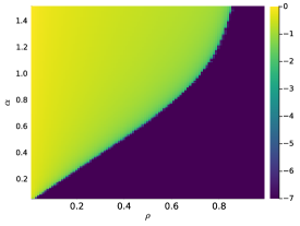
(a)

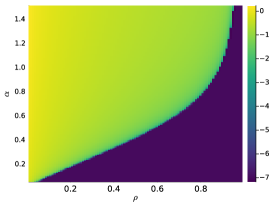
(b)

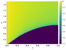
(c)

Figure 4: The optimal regularization parameter $\log_{10}\lambda$ for the bootstrap averaged unbiased estimator are plotted against the sparsity of the true signal $\rho$ and the measurement ratio $\alpha=M/N$ as a heat map. The measurement noise is set as $\Delta=0.15$.

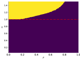
(a)

(b)

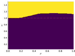
(c)

Figure 5: The typical number of unique samples in each bootstrap sample $\alpha(1-e^{-\mu_{B}^{\star}})$ scaled by $N$ is visualized. In the purple region, $\alpha(1-e^{-\mu_{B}^{\star}})<1$, and in the yellow region, $\alpha(1-e^{-\mu_{B}^{\star}})\geq 1$. The red dashed line shows $\alpha=1$. $\Delta=0.15$.

V-C Phase transition to an ensemble of interpolators

Fig. 4 shows the optimal regularization strength $\lambda^{\star}$ for $\hat{\sigma}^{2}$. Panels (a) and (b) show the results when the $\ell_{1}$-ratio is fixed, and panel (c) shows when the $\ell_{1}$-ratio is optimized. In all cases, it is clear that a phase transition has occurred in which $\lambda^{\ast}$ drops to an infinitesimally small value (although for numerical reasons, $\lambda$ is constrained to exceed $10^{-7}$) as the measurement ratio $\alpha$ decreases or $\rho$ increases. Moreover, Fig. 5 shows $\alpha(1-\mu_{B}^{\star})$, the typical number of unique data points in each bootstrap sample scaled by $N$: $\lim_{M,N\to\infty}(M\mu_{B})/N$. From Fig. 5, it is clear that the typical number of unique data points is always smaller than $1$ in the region where $\lambda^{\star}\simeq+0$. This holds, even if the measurement ratio $\alpha>1$. Thus, when $\lambda^{\star}\simeq+0$, the elastic net estimator in (8) becomes the minimum elastic net norm estimator as

$$\hat{\mathbf{\boldsymbol{w}}}^{\ast}=\min_{\mathbf{\boldsymbol{w}}\in\mathbb{R}^{N}}\sum_{i=1}^{N}\gamma|w_{i}|+\frac{1-\gamma}{2}w_{i}^{2},\,{\rm subject\,to}\\ \quad\mbox{1}\mbox{l}[c_{\mu}>0](y_{\mu}-\mathbf{\boldsymbol{x}}_{\mu}^{\top}{w})=0,\,\mu=1,2,\dots,M,$$ (14)

which is commonly known as minimum elastic net norm interpolator in machine learning [15, 16, 17]. These suggest that when elastic net regularization cannot determine an appropriate sparse structure of $\mathbf{\boldsymbol{w}}_{0}$, it is better to use an over-parameterized setting in which the number of unique data points of each bootstrap data is smaller than the dimension of $\mathbf{\boldsymbol{w}}_{0}$ and use an ensemble of interpolators.

VI Summary and discussion

In this study, we investigated the behavior of the bootstrap-averaged unbiased estimator of GAMP using AMPR and its SE. We found that the bootstrap averaging procedure can effectively reduce the variance of the unbiased estimator when the actual data generation process is inconsistent with the sparsity assumption of the regularization and the data size is insufficient. We also found a phase transition where the regularization strength drops to infinitesimally small values by decreasing the measurement ratio $\alpha$ or increasing $\rho$.

Although increasing the variance of weak learners is key to the success of ensemble learning [22, 23, 24], the phase transition to an ensemble of interpolators may be unexpected. Investigating whether similar phase transitions occur in other more sophisticated machine-learning models, such as neural networks, would be an interesting future direction.

We also remark that the landscape in $(\mu_{B},\lambda)$-space may not be convex in general. Thus, the uniqueness of the optimizer should be investigated in the future, paying attention to the relationship with the implicit regularization [25, 26, 27].

On the technical side, the key to this study was the precise performance characterization of the averaged estimator by AMPR, which was developed by combining GAMP and the replica method of statistical physics [28, 29]. Such a combination of approximate inference algorithms and the replica method has been used to develop approximate computation algorithms [13, 30, 14, 31, 32, 33, 34] and has not been applied to precise performance analysis of ensemble methods. It would be an interesting direction to try similar performance analysis for other bootstrap methods or ensemble learning.

References

• [1] S. Rangan, “Generalized approximate message passing for estimation with random linear mixing,” in 2011 IEEE International Symposium on Information Theory Proceedings.   IEEE, 2011, pp. 2168–2172.
• [2] A. Javanmard and A. Montanari, “State evolution for general approximate message passing algorithms, with applications to spatial coupling,” Information and Inference: A Journal of the IMA, vol. 2, no. 2, pp. 115–144, 2013.
• [3] P. Sur and E. J. Candès, “A modern maximum-likelihood theory for high-dimensional logistic regression,” Proceedings of the National Academy of Sciences, vol. 116, no. 29, pp. 14 516–14 525, 2019.
• [4] A. Javanmard and A. Montanari, “Hypothesis testing in high-dimensional regression under the gaussian random design model: Asymptotic theory,” IEEE Transactions on Information Theory, vol. 60, no. 10, pp. 6522–6554, 2014.
• [5] T. Takahashi and Y. Kabashima, “A statistical mechanics approach to de-biasing and uncertainty estimation in lasso for random measurements,” Journal of Statistical Mechanics: Theory and Experiment, vol. 2018, no. 7, p. 073405, 2018.
• [6] P. Sur, Y. Chen, and E. J. Candès, “The likelihood ratio test in high-dimensional logistic regression is asymptotically a rescaled chi-square,” Probability theory and related fields, vol. 175, no. 1, pp. 487–558, 2019.
• [7] A. Sakata and T. Obuchi, “Perfect reconstruction of sparse signals with piecewise continuous nonconvex penalties and nonconvexity control,” Journal of Statistical Mechanics: Theory and Experiment, vol. 2021, no. 9, p. 093401, 2021.
• [8] L. Zheng, A. Maleki, H. Weng, X. Wang, and T. Long, “Does $\ell_{p}$-minimization outperform $\ell_{1}$-minimization?” IEEE Transactions on Information Theory, vol. 63, no. 11, pp. 6896–6935, 2017.
• [9] B. Efron, “Bootstrap Methods: Another Look at the Jackknife,” The Annals of Statistics, vol. 7, no. 1, pp. 1 – 26, 1979. [Online]. Available: https://doi.org/10.1214/aos/1176344552
• [10] Z.-H. Zhou, Ensemble methods: foundations and algorithms.   CRC press, 2012.
• [11] K. P. Murphy, Probabilistic machine learning: an introduction.   MIT press, 2022.
• [12] H. Zou and T. Hastie, “Regularization and variable selection via the elastic net,” Journal of the royal statistical society: series B (statistical methodology), vol. 67, no. 2, pp. 301–320, 2005.
• [13] T. Obuchi and Y. Kabashima, “Semi-analytic resampling in lasso,” The Journal of Machine Learning Research, vol. 20, no. 1, pp. 2544–2576, 2019.
• [14] T. Takahashi and Y. Kabashima, “Semi-analytic approximate stability selection for correlated data in generalized linear models,” Journal of Statistical Mechanics: Theory and Experiment, vol. 2020, no. 9, p. 093402, 2020.
• [15] V. Muthukumar, K. Vodrahalli, V. Subramanian, and A. Sahai, “Harmless interpolation of noisy data in regression,” IEEE Journal on Selected Areas in Information Theory, vol. 1, no. 1, pp. 67–83, 2020.
• [16] P. L. Bartlett, P. M. Long, G. Lugosi, and A. Tsigler, “Benign overfitting in linear regression,” Proceedings of the National Academy of Sciences, vol. 117, no. 48, pp. 30 063–30 070, 2020.
• [17] T. Hastie, A. Montanari, S. Rosset, and R. J. Tibshirani, “Surprises in high-dimensional ridgeless least squares interpolation,” The Annals of Statistics, vol. 50, no. 2, pp. 949–986, 2022.
• [18] P. K. Mogensen and A. N. Riseth, “Optim: A mathematical optimization package for Julia,” Journal of Open Source Software, vol. 3, no. 24, p. 615, 2018.
• [19] P. Virtanen, R. Gommers, T. E. Oliphant, M. Haberland, T. Reddy, D. Cournapeau, E. Burovski, P. Peterson, W. Weckesser, J. Bright, S. J. van der Walt, M. Brett, J. Wilson, K. J. Millman, N. Mayorov, A. R. J. Nelson, E. Jones, R. Kern, E. Larson, C. J. Carey, İ. Polat, Y. Feng, E. W. Moore, J. VanderPlas, D. Laxalde, J. Perktold, R. Cimrman, I. Henriksen, E. A. Quintero, C. R. Harris, A. M. Archibald, A. H. Ribeiro, F. Pedregosa, P. van Mulbregt, and SciPy 1.0 Contributors, “SciPy 1.0: Fundamental Algorithms for Scientific Computing in Python,” Nature Methods, vol. 17, pp. 261–272, 2020.
• [20] T. Obuchi and Y. Kabashima, “Cross validation in lasso and its acceleration,” Journal of Statistical Mechanics: Theory and Experiment, vol. 2016, no. 5, p. 053304, 2016.
• [21] R. Tibshirani, “Regression shrinkage and selection via the lasso: a retrospective,” Journal of the Royal Statistical Society: Series B (Statistical Methodology), vol. 73, no. 3, pp. 273–282, 2011.
• [22] A. Krogh and P. Sollich, “Statistical mechanics of ensemble learning,” Physical Review E, vol. 55, no. 1, p. 811, 1997.
• [23] P. Sollich and A. Krogh, “Learning with ensembles: How overfitting can be useful,” Advances in neural information processing systems, vol. 8, 1995.
• [24] L. I. Kuncheva and C. J. Whitaker, “Measures of diversity in classifier ensembles and their relationship with the ensemble accuracy,” Machine learning, vol. 51, no. 2, pp. 181–207, 2003.
• [25] D. LeJeune, H. Javadi, and R. Baraniuk, “The implicit regularization of ordinary least squares ensembles,” in International Conference on Artificial Intelligence and Statistics.   PMLR, 2020, pp. 3525–3535.
• [26] J.-H. Du, P. Patil, and A. K. Kuchibhotla, “Subsample ridge ensembles: Equivalences and generalized cross-validation,” arXiv preprint arXiv:2304.13016, 2023.
• [27] T. Yao, D. LeJeune, H. Javadi, R. G. Baraniuk, and G. I. Allen, “Minipatch learning as implicit ridge-like regularization,” in 2021 IEEE International Conference on Big Data and Smart Computing (BigComp).   IEEE, 2021, pp. 65–68.
• [28] M. Mézard and A. Montanari, Information, physics, and computation.   Oxford University Press, 2009.
• [29] A. Montanari and S. Sen, “A short tutorial on mean-field spin glass techniques for non-physicists,” arXiv preprint arXiv:2204.02909, 2022.
• [30] T. Takahashi and Y. Kabashima, “Replicated vector approximate message passing for resampling problem,” arXiv preprint arXiv:1905.09545, 2019.
• [31] D. Malzahn and M. Opper, “An approximate analytical approach to resampling averages,” Journal of Machine Learning Research, vol. 4, no. Dec, pp. 1151–1173, 2003.
• [32] ——, “A statistical mechanics approach to approximate analytical bootstrap averages,” in Advances in Neural Information Processing Systems, 2003, pp. 343–350.
• [33] ——, “Approximate analytical bootstrap averages for support vector classifiers,” in Advances in Neural Information Processing Systems, S. Thrun, L. Saul, and B. Schölkopf, Eds., vol. 16.   MIT Press, 2003. [Online]. Available: https://proceedings.neurips.cc/paper/2003/file/2c6ae45a3e88aee548c0714fad7f8269-Paper.pdf
• [34] M. Opper, “An approximate inference approach for the pca reconstruction error,” Advances in Neural Information Processing Systems, vol. 18, 2005.