Neural Common Neighbor with Completion for Link Prediction

Abstract

Despite its outstanding performance in various graph tasks, vanilla Message Passing Neural Network (MPNN) usually fails in link prediction tasks, as it only uses representations of two individual target nodes and ignores the pairwise relation between them. To capture the pairwise relations, some models add manual features to the input graph and use the output of MPNN to produce pairwise representations. In contrast, others directly use manual features as pairwise representations. Though this simplification avoids applying a GNN to each link individually and thus improves scalability, these models still have much room for performance improvement due to the hand-crafted and unlearnable pairwise features. To upgrade performance while maintaining scalability, we propose Neural Common Neighbor (NCN), which uses learnable pairwise representations. To further boost NCN, we study the unobserved link problem. The incompleteness of the graph is ubiquitous and leads to distribution shifts between the training and test set, loss of common neighbor information, and performance degradation of models. Therefore, we propose two intervention methods: common neighbor completion and target link removal. Combining the two methods with NCN, we propose Neural Common Neighbor with Completion (NCNC). NCN and NCNC outperform recent strong baselines by large margins. NCNC achieves state-of-the-art performance in link prediction tasks. Our code is available at https://github.com/GraphPKU/NeuralCommonNeighbor.

1 Introduction

Link prediction is a crucial task in graph machine learning. It has various real-world applications, such as recommender systems (Zhang & Chen, 2020), knowledge graph completion (Zhu et al., 2021), and drug interaction prediction (Souri et al., 2022). Graph Neural Networks have been used in link prediction. Among these GNNs, Graph Autoencoder (GAE) (Kipf & Welling, 2016) is one representative method, which uses the representations of two target nodes produced by Message Passing Neural Network (MPNN) (Gilmer et al., 2017) to predict the existence of the link. GAE achieves good performance on some datasets. However, traditional link prediction heuristics, including Common Neighbor (CN) (Barabási & Albert, 1999), Resource Allocation (RA) (Zhou et al., 2009), and Adamic-Adar (AA) (Adamic & Adar, 2003), sometimes can outperform GAE/MPNN by large margins (Zhang et al., 2021). Therefore, recent works have been trying to boost GNNs for link prediction (Zhang & Chen, 2018; Zhu et al., 2021; Yun et al., 2021; Chamberlain et al., 2022).

Zhang et al. (2021) notice that GAE only uses node representations and ignores pairwise relations between target nodes. For example, in Figure 1, MPNN will produce exactly equal representations for node $v_{2},v_{3}$ as they are symmetric in the graph. So GAE will produce the same prediction for two links $(v_{1},v_{2})$ and $(v_{1},v_{3})$. However, their pairwise relations are different. For example, $v_{1}$ and $v_{2}$ have a common neighbor $v_{4}$, while $v_{1}$ and $v_{3}$ do not have any. This suggests the key to boost MPNNs is capturing pairwise relations.

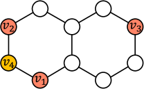
Figure 1: The failure of MPNN in link prediction task. $v_{2}$ and $v_{3}$ have equal MPNN node representations due to symmetry. However, with different pairwise relations, $(v_{1},v_{2})$ and $(v_{1},v_{3})$ should have nonequal representations.

Existing works boosting MPNNs vary in how they capture pairwise representations. SEAL (Zhang & Chen, 2018) adds target-link-specific hand-crafted features to the node features and modifies the input graph of MPNN, whose output node representations are then pooled to produce pairwise representations. Though it outperforms GAE significantly, SEAL has to rerun MPNN on a different graph for each target link, leading to high computation overhead. To accelerate it, Neo-GNN (Yun et al., 2021) and BUDDY (Chamberlain et al., 2022) decouple the pairwise representations from node representation learning. They directly use manual features as pairwise representations and only run MPNN on the original graph. Therefore, these models need to run MPNN only once for all target links and scale much better. However, their pairwise representations are oversimplified and still have much room for improvement.

To upgrade performance, we propose Neural Common Neighbor (NCN). Similar to Neo-GNN and BUDDY, NCN runs MPNN on the original graph for node representations. However, instead of using hand-crafted features, NCN uses learnable and flexible pairwise representations, which sum common neighbors’ node representations produced by MPNN. In experiments, NCN maintains scalability and outperforms existing models.

As our second contribution, we analyze how the incompleteness of the input graph affects link prediction. Incompleteness of input graph is ubiquitous for link prediction, as the task itself is to predict unobserved edges which do not exist in the input graph. In this work, we empirically find that incompleteness leads to distribution shift between the training and test set and loss of common neighbor information. We intervene in the incompleteness to solve this problem. Specifically, we focus on two graph structural properties crucial to NCN, namely common neighbor and the existence of target link, and propose two intervention methods: Common Neighbor Completion (CNC) and Target Link Removal (TLR). CNC iteratively completes unobserved links with a link prediction model. TLR removes the target links from the input graph. In experiments, our intervention methods further improve the performance of NCN.

In conclusion, our contributions are as follows:

• We propose Neural Common Neighbor (NCN) to boost link prediction with learnable pairwise representations. NCN outperforms existing models and maintains the scalability.

• We analyze how graph incompleteness hampers link prediction models. To alleviate the unobserved link problem, we intervene in the incompleteness and propose two methods: target link removal and common neighbor completion.

• With these methods, we further improve NCN and propose Neural Common Neighbor with Completion (NCNC). NCNC achieves state-of-the-art performance in link prediction tasks.

2 Preliminaries

We consider an undirected graph ${\mathcal{G}}=(V,E,A,X)$, where $V=\{1,2,\ldots,n\}$ is the set of $n$ nodes, $E\subseteq V\times V$ is the set of edges, $X\in\mathbb{R}^{n\times F}$ is node feature matrix whose $v$-th row $X_{v}$ is of node $v$, and adjacency matrix $A\in\mathbb{R}^{n\times n}$ is a symmetric matrix and defined as follows

$$A_{uv}=\begin{cases}1&\text{ if }(u,v)\in E,\\ 0&\text{ otherwise.}\end{cases}$$ (1)

where $1$ can also be replaced with edge weight. The degree of node $u$ is $d(u,A):=\sum_{v=1}^{n}A_{uv}$. Node $u$’s neighbors are nodes connected to $u$, $N(u,A):=\{v|v\!\in\!V,A_{uv}>0\}$. For simplicity of notations, we use $N(u)$ to denote $N(u,A)$ when $A$ is fixed. Common neighbor means nodes connected to both $i$ and $j$: $N(i)\bigcap N(j)$.

High Order Neighbor of Graph.

We define $A^{l}$ as the adjacency matrix of the high-order graph, where $v$ is a neighbor of $u$ if there is a walk of length $l$ between them in the original graph. $N(u,A^{l})=\{v|v\!\in\!V,A^{l}_{uv}>0\}$ denotes the set of $u$’s neighbors in the high-order graph. $N_{l}(u,A)$ denotes the set of nodes whose shortest path distance to $u$ in graph $A$ is $l$. Existing works define high-order neighbors as either $N(u,A^{l})$ or $N_{l}(u,A)$. Most generally, the neighborhood of $u$ can be expressed as $N_{l_{1}}(u,A^{l_{2}})$, returning all nodes with shortest path distance $l_{1}$ to $u$ in the high-order graph $A^{l_{2}}$. For simplicity of notations, we use $N_{l_{1}}^{l_{2}}(u)$ to denote $N_{l_{1}}(u,A^{l_{2}})$ when $A$ is fixed, and let $N^{l}(u)=N_{1}^{l}(u)$, $N_{l}(u)=N_{l}^{1}(u)$. Given a target link $(i,j)$, their neighborbood overlap is given by $N_{l_{1}}^{l_{2}}(i)\bigcap N_{l_{1}^{\prime}}^{l_{2}^{\prime}}(j)$, and their neighborhood difference is given by $N_{l_{1}}^{l_{2}}(i)-N_{l_{1}^{\prime}}^{l_{2}^{\prime}}(j)$.

Message Passing Neural Network.

Message passing neural network (MPNN) (Gilmer et al., 2017), composed of message passing layers, is a common GNN framework. The $k^{\text{th}}$ layer ($k=1,2,...,K$) can be formulated as follows.

$${\bm{h}}_{v}^{(k)}=U^{(k)}({\bm{h}}_{v}^{(k-1)},\text{AGG}(\\ \{M^{(k)}({\bm{h}}_{v}^{(k-1)},{\bm{h}}_{u}^{(k-1)})|u\in N(v)\})),$$ (2)

where ${\bm{h}}_{v}^{(k)}$ is the representation of node $v$ at the $k^{\text{th}}$ layer, $U^{(k)},M^{(k)}$ are some functions like multi-layer perceptron (MLP), and AGG denotes an aggregation function like sum and max. For each node, a message passing layer aggregates information from neighbors to update the representation of the node. The initial node representation ${\bm{h}}_{v}^{(0)}$ is node feature $X_{v}$. Node representations produced by MPNN are the output of the last message passing layer, $\text{MPNN}(v,A,X)={\bm{h}}_{v}^{(K)}$.

3 Related Work

3.1 Link Prediction Heuristics

Research on developing hand-crafted graph structure features (heuristics) for link prediction has been longstanding before GNN methods (Liben-Nowell & Kleinberg, 2003). The most relevant heuristics to our paper are Common Neighbor (CN) (Barabási & Albert, 1999), Resource Allocation (RA) (Zhou et al., 2009), and Adamic Adar (AA) (Adamic & Adar, 2003). Given an graph and a link $(i,j)$ in it, they produce a score $S(i,j)$ by pooling representations of the common neighbors of $i$ and $j$. Links with higher scores are more likely to exist. Equations 3 show the score function used in these different heuristics.

$$S_{\text{CN}}(i,j) =\sum_{u\in N(i)\bigcap N(j)}1,$$ (3a)

$$S_{\text{RA}}(i,j) =\sum_{u\in N(i)\bigcap N(j)}\frac{1}{d(u)},$$ (3b)

$$S_{\text{AA}}(i,j) =\sum_{u\in N(i)\bigcap N(j)}\frac{1}{\log d(u)}.$$ (3c)

Specifically, CN simply uses $1$ as the node representation, while RA and AA further use node degree information and usually outperform CN.

3.2 GNNs for Link Prediction

Another research direction is using graph neural networks for link prediction, where Graph Autoencoder (GAE) (Kipf & Welling, 2016) is the representative one. It predicts an edge with node embeddings produced by MPNN as follows,

$$\hat{A}_{ij}=\text{sigmoid}(\text{MPNN}(i,A,X)^{T}\text{MPNN}(j,A,X)),$$ (4)

where $\hat{A}_{ij}$ is the existence probability of link $(i,j)$ predicted by GAE. Note that GAE ignores pairwise relations completely as we have shown in Section 1 and Figure 1, so CN, RA, and AA outperform GAE in many datasets.

Recently, many methods have been proposed to help GNNs to capture pairwise relations. SEAL (Zhang & Chen, 2018) adds target-link-specific distance features to the input graph of MPNN and outperforms GAE, CN, RA, and AA significantly. However, SEAL suffers from high computation overhead. Unlike GAE, which only needs to run MPNN once to predict all target links, SEAL must rerun MPNN for each target link.

To improve the scalability, Yun et al. (2021) and Chamberlain et al. (2022) directly add manual pairwise features to the node representations produced by MPNN instead of modifying the input graph of MPNN. Inspired by traditional heuristics, Neo-GNN (Yun et al., 2021) further utilizes high-order neighborhood overlaps and, moreover, uses a learnable node degree function instead of the fixed functions in RA and AA, which leads to significant outperformance over the heuristics. Another recent method is called BUDDY (Chamberlain et al., 2022), which further distinguishes the pairwise feature as the overlap feature and difference feature, but ignores node degree information as CN.

Both Neo-GNN and BUDDY only run MPNN once and achieve similar computation overhead to GAE. However, one key limitation is that their pairwise features are hardly learnable and therefore inflexible. Additionally, they are completely decoupled from the node features/representations produced by the MPNN. These problems restrict their performance.

3.3 Incompleteness of Graph

As the link prediction task is to predict unobserved edges, the observed graph is deemed to be incomplete. However, existing methods relying heavily on graph structures such as CN might behave very differently under different graph completeness levels. Some existing works also notice this problem. Yang et al. (2022) analyze how unobserved links distort the evaluation score. They focus on metrics and benchmark design. In contrast, we for the first time study the performance degradation caused by incompleteness as well as how to alleviate it. Different from our settings, Das et al. (2020) study unobserved nodes and propose an inductive learning method. Their method uses no intervention method and is completely different from ours.

4 Neural Common Neighbor

Recent link prediction models use manual and inflexible pairwise features, which restrict their performance and generalization. In this section, we first propose a more general framework, which can include the heuristics introduced in Section 3.1 as well as Neo-GNN and BUDDY in Section 3.2. Then, based on the framework, we propose a realization called Neural Common Neighbor (NCN) by replacing the manual features with an MPNN to achieve better capacity.

Table 1: How the general framework shown in Equation (9) include several models.

	Model	Neighbor selection	Set operator $\oplus$	$g(x)$	$f(x)$
Heuristics	CN	First-order	Intersection	$1$	$1$
	RA	First-order	Intersection	$1$	$1/x$
	AA	First-order	Intersection	$1$	$1/\log(x)$
GNN	Neo-GNN	High-order	Intersection	$x$	MLP
	BUDDY	High-order	Intersection & Difference	$1$	$1$
	NCN	First-order	Intersection	$1$	MPNN

4.1 A General Framework of Pairwise Feature

Neo-GNN uses the higher-order pairwise feature, which is a weighted summation in different high-order neighborhood as shown in Equation (5).

$$s(i,j,A)=\sum_{l_{1}=1}^{l}\sum_{l_{2}=1}^{l}\beta^{l_{1}+l_{2}-2}z_{l_{1}l_{2}}(i,j,A),$$ (5)

where $l$ and $\beta$ are hyperparameters, and $z_{l_{1}l_{2}}$ is the feature from high-order neighbors $N^{l_{1}}(i)$ and $N^{l_{2}}(j)$ defined as follows.

$$z_{l_{1}l_{2}}(i,j,A)=\sum_{u\in N^{l_{1}}(i)\bigcap N^{l_{2}}(j)}A^{l_{1}}_{iu}A^{l_{2}}_{ju}f(d(u)),$$ (6)

where $f$ is a learnable function of node degree $d(u)$. The pairwise feature $z_{l_{1}l_{2}}(i,j,A)$ pools degree features of nodes within high-order neighborhood overlap.

BUDDY further uses the high-order difference feature. The pair-wise feature is composed of $k^{2}$ overlap features and $2k$ difference features as follows.

$$\{a_{l_{1},l_{2}}(i,j)\left|l_{1},l_{2}\in[k]\right.\}\bigcup\{b_{l}(i,j),b_{l}(j,i)\left|l\in[k]\right.\}$$ (7)

where $k$ is a hyperparameter, and functions $a$ and $b$ measure high-order neighborhood overlaps and differences, respectively, which are defined as follows.

$$a_{l_{1},l_{2}}(i,j) =\sum_{u\in N_{l_{1}}(i)\bigcap N_{l_{2}}(j)}1,$$ (8a)

$$b_{l}(i,j) =\sum_{u\in N_{l}(i)-\bigcup_{l^{\prime}=1}^{k}N_{l^{\prime}}(j)}1.$$ (8b)

How to use the pairwise feature is the key to link prediction models. Let’s focus on the form of the pairwise feature: score function $S(i,j,A)$ in heuristics, the high-order overlap feature $z_{l_{1}l_{2}}(i,j,A)$ in Neo-GNN, and high-order overlap feature $a_{l_{1},l_{2}}$ and difference feature $b_{l}$ in BUDDY. All these features can be summarized into the following general framework

$$\sum_{u\in N_{l_{1}}^{l_{2}}(i)\oplus N_{l_{1}^{\prime}}^{l_{2}^{\prime}}(j)}g(A^{l_{2}}_{iu})g(A^{l_{2}^{\prime}}_{ju})f(d(u)),$$ (9)

where $N_{l_{1}}^{l_{2}}(i)$ and $N_{l_{1}^{\prime}}^{l_{2}^{\prime}}(j)$ denote the general neighborhood of $i$ and $j$ respectively, $\oplus$ is a set operator, and $f,g$ are node (degree) and weight functions, respectively. Table 1 shows how the general framework contains the three heurisitics CN, RA and AA as well as the two GNN models, Neo-GNN and BUDDY. Models using high-order neighbors are called high-order models and first-order models use first-order neighbors only.

4.2 Neural Common Neighbor

Now we introduce Neural Common Neighbor (NCN). We first notice that one of the main differences between existing models is the node function $f$. However, existing models all use inflexible constant or degree functions, which fail to capture more refined node features such as multi-hop structure and attribute information. Therefore, we propose to use MPNN to replace $f$, which leads to the following pairwise feature

$$\sum_{u\in N_{l_{1}}^{l_{2}}(i)\oplus N_{l_{1}^{\prime}}^{l_{2}^{\prime}}(j)}g(A^{l_{2}}_{iu})g(A^{l_{2}^{\prime}}_{ju})\text{MPNN}(u,A,X).$$ (10)

MPNN is a more powerful and flexible feature extractor than manually-designed degree-based feature functions. Theoretically, because MPNN can fit arbitrary degree functions $f(d(u))$ (Xu et al., 2019), this model is strictly more powerful than the heuristics, Neo-GNN and BUDDY.

The next question is the selection of the neighborhood and the set operator $\oplus$. Surprisingly, we find the improvement given by explicit higher-order neighbors is marginal after we import the MPNN (see Section 6.3). We believe that it is because the higher-order information could be implicitly learned by the MPNN. Considering the scalability, we choose to only keep the first-order neighbor and set the operator only to intersection, which leads to our NCN model:

$$\text{NCN}(i,j,A,X)=\sum_{u\in N(i)\bigcap N(j)}\text{MPNN}(u,A,X),$$ (11)

where $g(A_{iu})$ and $g(A_{ju})$ are constants and ignored.

As our first contribution, NCN is a simple but powerful model to capture pairwise features. It is an implicit high-order model by aggregating first-order common neighbors each has its higher-order information implicitly learned by an MPNN. This trick effectively controls the model’s time complexity, making it close to Neo-GNN and BUDDY but having a more powerful and flexible feature extractor. More analysis on time complexity can be found in Appendix C.

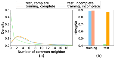
(a)

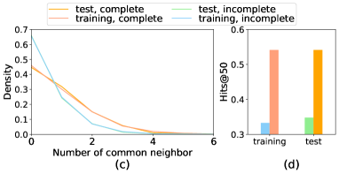
(b)

Figure 2: Visualization of incompleteness on datasets. The incomplete graph only contains edges in the training set, and the complete graph further contains edges in the validation and test set. (a) and (b) visualize the ogbl-collab dataset. (c) and (d) visualize the Cora dataset. (a) and (c) are for distributions of the number of common neighbors of the training edges and test edges. (b) and (d) show performance of CN on the training set and test set.

5 Neural Common Neighbor with Completion

Incompleteness of graph is ubiquitous in link prediction tasks, as the task is to predict unobserved edges. However, few works have studied this problem. This section first shows that the incompleteness may lead to distribution shifts between the training and test sets, loss of common neighbor information, and therefore performance degradation of models. Then, we intervene in the incompleteness and propose two methods, namely common neighbor completion and target link removal. With these intervention methods, we further improve NCN and propose Neural Common Neighbor with Completion (NCNC).

5.1 Incompleteness Visualization

Assume the graph only containing edges in the training set is the input incomplete graph, while the graph containing edges in the training, validation and test sets is the ground-truth complete graph. We focus on the following questions:

(1) What is different between the complete and incomplete graphs, and (2) whether the difference leads to performance degradation?

To answer these questions, we investigate two common datasets: ogbl-collab (Hu et al., 2020) and Cora (Yang et al., 2016). Because the common neighbor information is crucial for link prediction as well as our NCN model, we visualize the distribution of the number of common neighbors of training/test edges in the complete/incomplete graphs separately. Firstly, by comparing the blue and green lines in Figure 2(a), we find there is a significant distribution shift between the training and test sets in the incomplete graph of the ogbl-collab dataset, and the shift disappears when the graph is complete (the red and orange lines), which suggests this shift is due to the incompleteness. Such a significant distribution shift between training and test links in the input graph might cause difficulty in model generalization.

In contrast, there is no such distribution shift between training and test edges in Cora (Figure 2(c)). The reason could be due to the different dataset split methods. Obgl-collab splits the training and test edges according to the timestamp of edges, and the edges of the test set are all in the same year. Thus, edges in the test set will have stronger correlations with other test edges than with edges in the training set. Therefore, the test edges may have fewer common neighbors in the incomplete graph than the training edges. On the contrary, the Cora dataset randomly chooses the test set and thus avoids the distribution shift.

Another phenomenon is the decrease of test edges’ common neighbors in the incomplete graph, which can be see by the blue and green lines in Figure 2(c). Comparing the incomplete and complete graphs for the same training/test set, there are fewer common neighbors in the incomplete graph, which indicates loss of common neighbor information due to the incompleteness.

In conclusion, for the first question, the incompleteness could lead to at least the following two problems:

• Distribution shift: with certain dataset splits, there could be a distribution shift between the training and test sets due to the incompleteness.

• Loss of common neighbor information: there could be fewer common neighbors in the incomplete graph.

Remark.   On the one hand, we acknowledge that there is no guarantee that these two phenomena fully account for the difference between complete and incomplete graphs. On the other hand, these two problems do not necessarily appear in every dataset, and the significance of these problems could also vary in different datasets according to the data type, generation method, data split, and so on.

To verify whether the incompletness causes performance degradation of link prediction models, we evaluate CN by ranking the training/test edges against the negative test links, under both complete and incomplete graphs, on both datasets. We also use Hits@K metrics as in  (Chamberlain et al., 2022). Though CN is not learnable and does not involve generalization, it has no data leakage problem, as CN computation for a target edge does not involve the edge itself. Moreover, CN can reveal how incompleteness changes the input graph structure of other learnable models, so it is a good reference here. The performance is shown in Figure 2(b) and (d). On both datasets, CN’s performance for test edges degrades a lot between complete and incomplete graphs (green and orange bars), which verifies the performance degradation. This phenomenon indicates that we could have gotten a much better link prediction model if the input graph were more complete.

Comparing the blue and green bars in Figure 2(b) (ogbl-collab) and Figure 2(d) (Cora), we see that there is a huge performance difference between training and test sets in the incomplete ogbl-collab, which disappears in the incomplete Cora. This aligns well with the distribution shift problem discussed above, which is less significant under random data split.

In conclusion, the incompleteness problem leads to distribution shift and loss of common neighbor information and causes performance degradation of link prediction models. In practice, we can never really evaluate CN in the complete graph but only in the incomplete input graph. Thus, the above phenomena need other alleviation methods, which will be discussed in later subsections.

5.2 Common Neighbor Completion

Motivated by the above analysis, our strategy is to first complement the input graph softly using a link prediction model (intervention on the incompleteness), and then apply the model again on the more complete graph to give final predictions. We use NCN as the link prediction model. To illustrate our model, we use the causal graphs (Judea, 2009) in Figure 3(a) and 3(b). In Figure 3(a), $\tilde{A}$ denotes the ground-truth complete graph, $T_{ij}$ is a random variable determining link $(i,j)$’s incompleteness ($T_{ij}\!=\!1$ means link $(i,j)$ is missing from the complete graph), and $\tilde{A},T_{ij}$ together determine the link existence $A_{ij}$ in the input graph. In Figure 3(b), $Y_{uij}$ is a random variable indicating whether node $u$ is a common neighbor of $(i,j)$ in the input graph, which is determined by $T_{iu},T_{ju},\tilde{A}$ together.

To alleviate the incompleteness, we intervene in $T$ by setting $T_{iu}\!=\!T_{ju}\!=\!0$, so that $A_{iu}\!=\!\tilde{A}_{iu},A_{ju}\!=\!c$, i.e., we want to use the edges $(i,u)$ and $(j,u)$ in the complete graph to compute the common neighbor $Y_{uij}$. However, since $\tilde{A}_{iu}$ and $\tilde{A}_{ju}$ are unknown, we choose to predict them using NCN first. Instead of predicting the existence, we let NCN output a probability instead, and the final probability of $u$ being a common neighbor of $(i,j)$ is modeled as follows:

$$P_{uij}=\begin{cases}1&\text{if }u\!\in\!N(i,\!A)\bigcap N(j,\!A)\\ \sigma(\text{NCN}(i,u,A,X))&\text{if }u\!\in N(j,\!A)\!-\!N(i,\!A)\\ \sigma(\text{NCN}(j,u,A,X))&\text{if }u\!\in\!N(i,\!A)\!-\!N(j,\!A)\\ 0&\text{otherwise }\end{cases}$$ (12)

where $\sigma$ is the sigmoid function. If both edges $(i,u)$ and $(j,u)$ are observed, $u$ must be a common neighbor of $i,j$. If one of $(i,u)$ and $(j,u)$ is unobserved, we use NCN to predict its link existence probability, which is also used as the probability of $u$ being a common neighbor. The fourth case where both $(i,u)$ and $(j,u)$ are unobserved has a much less probability, so we just set the probability to $0$.

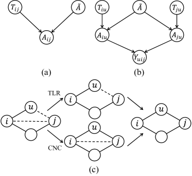
Figure 3: (a) Causal graph of the link existence and incompleteness. (b) Causal graph of common neighbor and incompleteness. $T$: Edge incompleteness variable. $T=0$: edge is observed. $T=1$: edge is unobserved. $T$ varies with the target link. $\tilde{A}$: the complete graph. Edge incompleteness and the complete graph jointly determine the observed graph. $A_{ab}$: the existence of link $(a,b)$ in the observed graph. $Y_{uij}$: whether $u$ is a common neighbor of $(i,j)$ in the observed graph. $Y_{uij}=1$ iff both links $(i,u)$ and $(j,u)$ exist. (c) An example of our two intervention methods. $(i,j)$ is the target link. Solid lines mean observed edges. Dotted lines mean links in the full graph affected by incompleteness. $(i,j)$ and $(u,j)$ are observed in the training set while unobserved in the test set. TLR (target link removal) removes the target link $(i,j)$. CNC (common neighbor completion) completes the observed graph and thus transforms the dotted line $(u,j)$ into a solid line. With the two methods, dotted lines are eliminated, and the incompleteness problem is alleviated.

We call the above intervention trick Common Neighbor Completion (CNC). In fact, it can be combined with any link prediction method. After CNC, we apply NCN again to the “completed” graph where soft common neighbor weight $P_{uij}$ is used, leading to the final model which we call Neural Common Neighbor with Completion (NCNC):

$$\text{NCNC}(i,j,A,X)=\sum_{u\in V}P_{uij}\text{MPNN}(u,A,X).$$ (13)

Furthermore, this strategy can be extended to a iterative algorithm. Starting from the original graph $A^{(0)}=A$, we iteratively complete the graph to get the $A^{(k)}$ from $A^{(k-1)}$ until the final iteration $K$. We call this model NCNC with maximum number of iterations $K$ (NCNC-$K$). For the first iteration $k=0$, NCNC-$0$ is the same as NCN. At iteration $k>0$, NCNC-$k$ of the target link $(i,j)$, denoted by $\text{NCNC}(i,j,A^{(k)},X)$, has the following form

$$\!\!\sum_{u\!\in\!N(i,\!A)\bigcap\atop N(j,\!A)}\!\!h_{u}+\!\!\sum_{u\!\in\!N(j,\!A)-\atop N(i,\!A)}\!\!\hat{A}_{iu}^{(k-1)}h_{u}+\!\!\sum_{u\!\in\!N(i,\!A)-\atop N(j,\!A)}\!\!\hat{A}_{ju}^{(k-1)}h_{u}.$$ (14)

where $\hat{A}_{ab}^{(k-1)}=\text{NCNC}(a,b,A^{(k-1)},X)$ is the link existence probability produced by NCNC at iteration $k-1$, and $h_{u}$ is the node representation of $u$ produced by MPNN.

The time complexity of NCNC-$K$ is loosely bounded by $d^{K}$ times of NCN, where $d$ is the maximum node degree. More analysis can be found in Appendix C. In practice, $K=1$ is enough for most datasets.

5.3 Target Link Removal.

In Section 5.2, we pointed out that the incompleteness $T$ affects the common neighbor and degrades the performance of link prediction models. In this section, we will point out that the incompleteness will also affect the target link directly and cause bias between training and test sets. As shown in Figure 3(a), the complete graph and the incompleteness jointly determine the target link existence. Links in the training set are all observed ($T\!=\!0$), while other links to predict are all unobserved ($T\!=\!1$), leading to another distribution shift, which is different from the one we have shown in Section 5.1. However, in the test set, we cannot know whether the absence of the target link is due to the incompleteness $T\!=\!1$ or the actual ground-truth $\tilde{A}$. Thus, we cannot solve the problem by completing the graph. Therefore, we always intervene in $T$ of the target link and set it to $1$ in both the training and test sets, which is equivalent to always removing the target link $(i,j)$ from the input graph $A$ to get $\bar{A}$. We call this intervention trick Target Link Removal (TLR). Note that TLR is also used in previous works such as Zhang & Chen (2018) but never studied from a causal perspective. The total intervention strategy combining CNC and TLR is shown in Figure 3(c). We use the TLR trick in both NCN and NCNC models by just replacing $A$ with $\bar{A}$. In implementation, ideally we need to perform TLR for each link, but for scalability we simultaneously remove all edges in a batch from the input graph during the training stage. Experiments show that this method achieves up to $6\%$ performance gain in real-world tasks (see Section 6.3).

6 Experiment

Table 2: Results on link prediction benchmarks. The format is average score $\pm$ standard deviation. OOM means out of GPU memory.

	Cora	Citeseer	Pubmed	Collab	PPA	Citation2	DDI
Metric	HR@100	HR@100	HR@100	HR@50	HR@100	MRR	HR@20
CN	$33.92{\scriptstyle\pm 0.46}$	$29.79{\scriptstyle\pm 0.90}$	$23.13{\scriptstyle\pm 0.15}$	$56.44{\scriptstyle\pm 0.00}$	$27.65{\scriptstyle\pm 0.00}$	$51.47{\scriptstyle\pm 0.00}$	$17.73{\scriptstyle\pm 0.00}$
AA	$39.85{\scriptstyle\pm 1.34}$	$35.19{\scriptstyle\pm 1.33}$	$27.38{\scriptstyle\pm 0.11}$	$64.35{\scriptstyle\pm 0.00}$	$32.45{\scriptstyle\pm 0.00}$	$51.89{\scriptstyle\pm 0.00}$	$18.61{\scriptstyle\pm 0.00}$
RA	$41.07{\scriptstyle\pm 0.48}$	$33.56{\scriptstyle\pm 0.17}$	$27.03{\scriptstyle\pm 0.35}$	$64.00{\scriptstyle\pm 0.00}$	$49.33{\scriptstyle\pm 0.00}$	$51.98{\scriptstyle\pm 0.00}$	$27.60{\scriptstyle\pm 0.00}$
GCN	$66.79{\scriptstyle\pm 1.65}$	$67.08{\scriptstyle\pm 2.94}$	$53.02{\scriptstyle\pm 1.39}$	$44.75{\scriptstyle\pm 1.07}$	$18.67{\scriptstyle\pm 1.32}$	$84.74{\scriptstyle\pm 0.21}$	$37.07{\scriptstyle\pm 5.07}$
SAGE	$55.02{\scriptstyle\pm 4.03}$	$57.01{\scriptstyle\pm 3.74}$	$39.66{\scriptstyle\pm 0.72}$	$48.10{\scriptstyle\pm 0.81}$	$16.55{\scriptstyle\pm 2.40}$	$82.60{\scriptstyle\pm 0.36}$	$53.90{\scriptstyle\pm 4.74}$
SEAL	$81.71{\scriptstyle\pm 1.30}$	$83.89{\scriptstyle\pm 2.15}$	$75.54{\scriptstyle\pm 1.32}$	$64.74{\scriptstyle\pm 0.43}$	$48.80{\scriptstyle\pm 3.16}$	$87.67{\scriptstyle\pm 0.32}$	$30.56{\scriptstyle\pm 3.86}$
NBFnet	$71.65{\scriptstyle\pm 2.27}$	$74.07{\scriptstyle\pm 1.75}$	$58.73{\scriptstyle\pm 1.99}$	OOM	OOM	OOM	$4.00{\scriptstyle\pm 0.58}$
Neo-GNN	$80.42{\scriptstyle\pm 1.31}$	$84.67{\scriptstyle\pm 2.16}$	$73.93{\scriptstyle\pm 1.19}$	$57.52{\scriptstyle\pm 0.37}$	$49.13{\scriptstyle\pm 0.60}$	$87.26{\scriptstyle\pm 0.84}$	$63.57{\scriptstyle\pm 3.52}$
BUDDY	$88.00{\scriptstyle\pm 0.44}$	$\underline{92.93{\scriptstyle\pm 0.27}}$	$74.10{\scriptstyle\pm 0.78}$	$\underline{65.94{\scriptstyle\pm 0.58}}$	$49.85{\scriptstyle\pm 0.20}$	$87.56{\scriptstyle\pm 0.11}$	$78.51{\scriptstyle\pm 1.36}$
NCN	$\underline{89.05{\scriptstyle\pm 0.96}}$	${91.56{\scriptstyle\pm 1.43}}$	$\underline{79.05{\scriptstyle\pm 1.16}}$	$64.76{\scriptstyle\pm 0.87}$	$\underline{61.19{\scriptstyle\pm 0.85}}$	$\underline{88.64{\scriptstyle\pm 0.14}}$	$\underline{82.32{\scriptstyle\pm 6.10}}$
NCNC	$\mathbf{89.65{\scriptstyle\pm 1.36}}$	$\mathbf{93.47{\scriptstyle\pm 0.95}}$	$\mathbf{81.29{\scriptstyle\pm 0.95}}$	$\mathbf{66.61{\scriptstyle\pm 0.71}}$	$\mathbf{61.42{\scriptstyle\pm 0.73}}$	$\mathbf{89.12{\scriptstyle\pm 0.40}}$	$\mathbf{84.11{\scriptstyle\pm 3.67}}$

Table 3: Ablation analysis on link prediction benchmarks. The format is average score $\pm$ standard deviation.

	Cora	Citeseer	Pubmed	Collab	PPA	Citation2	DDI
Metric	HR@100	HR@100	HR@100	HR@50	HR@100	MRR	HR@20
CN	$33.92{\scriptstyle\pm 0.46}$	$29.79{\scriptstyle\pm 0.90}$	$23.13{\scriptstyle\pm 0.15}$	$56.44{\scriptstyle\pm 0.00}$	$27.65{\scriptstyle\pm 0.00}$	$51.47{\scriptstyle\pm 0.00}$	$17.73{\scriptstyle\pm 0.00}$
GAE	$89.01{\scriptstyle\pm 1.32}$	$91.78{\scriptstyle\pm 0.94}$	$78.81{\scriptstyle\pm 1.64}$	$36.96{\scriptstyle\pm 0.95}$	$19.49{\scriptstyle\pm 0.75}$	$79.95{\scriptstyle\pm 0.09}$	$61.53{\scriptstyle\pm 9.59}$
GAE+CN	$88.61{\scriptstyle\pm 1.31}$	$91.75{\scriptstyle\pm 0.98}$	$79.04{\scriptstyle\pm 0.83}$	$64.47{\scriptstyle\pm 0.14}$	$51.83{\scriptstyle\pm 0.58}$	$87.81{\scriptstyle\pm 0.06}$	$80.71{\scriptstyle\pm 5.56}$
NCN2	$88.87{\scriptstyle\pm 1.34}$	$91.36{\scriptstyle\pm 1.02}$	$80.21{\scriptstyle\pm 0.78}$	$65.43{\scriptstyle\pm 0.46}$	OOM	OOM	OOM
NCN-diff	$89.12{\scriptstyle\pm 1.04}$	$91.96{\scriptstyle\pm 1.23}$	$80.28{\scriptstyle\pm 0.88}$	$64.08{\scriptstyle\pm 0.40}$	$57.86{\scriptstyle\pm 1.26}$	$86.68{\scriptstyle\pm 0.16}$	$17.67{\scriptstyle\pm 8.70}$
NCN	$89.05{\scriptstyle\pm 0.96}$	$91.56{\scriptstyle\pm 1.43}$	$79.05{\scriptstyle\pm 1.16}$	$64.76{\scriptstyle\pm 0.87}$	$61.19{\scriptstyle\pm 0.85}$	$88.09{\scriptstyle\pm 0.06}$	$82.32{\scriptstyle\pm 6.10}$
NoTLR	$85.46{\scriptstyle\pm 1.65}$	$88.08{\scriptstyle\pm 1.23}$	$76.59{\scriptstyle\pm 1.33}$	$64.22{\scriptstyle\pm 0.49}$	$60.66{\scriptstyle\pm 0.63}$	$88.64{\scriptstyle\pm 0.14}$	$66.52{\scriptstyle\pm 11.37}$
NCNC	$89.65{\scriptstyle\pm 1.36}$	$93.47{\scriptstyle\pm 0.95}$	$81.29{\scriptstyle\pm 0.95}$	$66.61{\scriptstyle\pm 0.71}$	$61.42{\scriptstyle\pm 0.73}$	$89.12{\scriptstyle\pm 0.40}$	$84.11{\scriptstyle\pm 3.67}$
NCNC-2	$89.14{\scriptstyle\pm 0.84}$	$93.14{\scriptstyle\pm 0.96}$	$81.41{\scriptstyle\pm 1.07}$	$66.80{\scriptstyle\pm 0.43}$	$>24h$	$>24h$	$>24h$

In this section, we evaluate the performance of NCN and NCNC. Our code is available in the supplementary material. Detailed experimental settings are included in Appendix D.

We use seven link prediction benchmarks. Three are Planetoid citation networks: Cora, Citeseer, and Pubmed (Yang et al., 2016). Others are from Open Graph Benchmark (Hu et al., 2020): ogbl-collab, ogbl-ppa, ogbl-citation2, and ogbl-ddi. Their statistics and splits are shown in Appendix A.

6.1 Evaluation on Real-World Datasets

Our baselines include traditional heuristics: CN (Barabási & Albert, 1999), RA (Zhou et al., 2009), AA (Adamic & Adar, 2003); vanilla GNN with no pairwise feature: GCN (Kipf & Welling, 2017), SAGE (Hamilton et al., 2017); GNNs modifying the input graph of MPNN: SEAL (Zhang & Chen, 2018), NBFNet (Zhu et al., 2021); and GNNs with manual features as pairwise representations: Neo-GNN (Yun et al., 2021), BUDDY (Chamberlain et al., 2022). Their results are from  (Chamberlain et al., 2022). Our models are NCN and NCNC. We set the maximum number of iterations of NCNC to $1$. Their architectures are detailed in Appendix B.

Results are shown in Table 2. NCN beats all baselines on 5/7 datasets and achieves $5\%$ score increase on average compared with BUDDY, the most competitive baseline. On the two datasets left, NCN can still outperform all baselines other than BUDDY. NCN’s outstanding performance validates the advantage of learnable pairwise features over manual ones. NCNC further leads to $2\%$ performance gain, outperforming all baselines on all datasets. Notably, NCNC achives $61.42\%$ HR@100 on ogbl-ppa, outperforming the strongest baseline BUDDY by over $10\%$ absolute score.

Figure 4: Inference time and GPU memory on ogbl-collab. The process we measure includes preprocessing, MPNN, and predicting one batch of test links. As SEAL has out-of-memory problem with large batch sizes, we only use small batch sizes for SEAL.

6.2 Scalability

We compare the inference time and GPU memory on ogbl-collab in Figure 4. Our strongest baseline BUDDY (Chamberlain et al., 2022)’s code is not released so is not compared. NCN and NCNC have a similar computation overhead to GAE, as they both need to run MPNN only once. In contrast, SEAL, which reruns MPNN for each target link, takes $86$ times more time compared with NCN with a small batch size $2048$, and the disadvantage will be more significant with a larger batch size. To our surprise, Neo-GNN is even slower than SEAL, even if it only needs to run MPNN once. The reason is that it uses pairwise features that are much more complex and time-consuming than CN. We also conduct scalability comparison on other datasets and observe the same results (see Appendix E).

6.3 Ablation Analysis

To validate the design of Neural Common Neighbor, we conduct a thorough ablation analysis (see Table 3).

GAE uses node representations only. GAE+CN further utilizes CN as pairwise features. On OGB datasets, GAE+CN outperforms GAE by $70\%$, and NCN further achieves $5.5\%$ higher score than GAE+CN, which implies that the learnable pairwise representations we propose are effective. On Planetoid datasets though, the improvement is minimal, which indicates that these datasets require less common neighbor information.

NCN-diff is NCN plus neighborhood difference information, and NCN2 is NCN with high-order neighborhood overlap. For a target link $(i,j)$, compared with NCN, NCN-diff further sums representations of nodes in $N(i,A)-N(j,A)$ and $N(j,A)-N(i,A)$, and NCN2 further uses $N(i,A^{2})\bigcap N(j,A)$ and $N(i,A)\bigcap N(j,A^{2})$. As we can see, NCN, NCN-diff and NCN2 have similar performance on most datasets, verifying that first-order neighborhood overlap may be enough. The low score of NCN-diff on DDI might be because the DDI’s high node degree makes neighborhood difference noisy and uninformative.

NoTLR is NCN without TLR. On average, TLR leads to $6\%$ performance gain. NCNC-2 is NCNC with maximum number of iterations $2$. It achieves similar performance to NCNC. Therefore, setting maximum number of iterations to $1$ is enough for our datasets. Both intervention methods boost NCN significantly.

7 Conclusion

We propose Neural Common Neighbor (NCN), a scalable and powerful model for link prediction leveraging learnable pairwise features. Furthermore, we study the graph incompleteness problem. By visualizing the distribution shift and performance degradation caused by incompleteness, we propose two tricks, target link removal and common neighbor completion. Combining NCN with the two tricks, our final model NCNC outperforms state-of-the-art baselines on all the datasets in both speed and performance.

Appendix A Dataset Statistics

The statistics of each dataset are shown in Table 4.

Table 4: Statistics of dataset.

	Cora	Citeseer	Pubmed	Collab	PPA	DDI	Citation2
#Nodes	2,708	3,327	18,717	235,868	576,289	4,267	2,927,963
#Edges	5,278	4,676	44,327	1,285,465	30,326,273	1,334,889	30,561,187
splits	random	random	random	fixed	fixed	fixed	fixed
average degree	3.9	2.74	4.5	5.45	52.62	312.84	10.44

Random splits use $70\%/10\%/20\%$ edges for training/validation/test set respectively. Different from others, the collab dataset allows using validation edges as input on test set.

Appendix B Model Architecture

This section concludes our methods in Section 4 and Section 5.

Given an input graph $A$, a node feature matrix $X$, and target links $\{(i_{1},j_{1}),(i_{2},j_{2}),...,(i_{t},j_{t})\}$, our models consist of three steps: target link removal, MPNN, and predictor. NCN and NCNC only differ in the last step.

Target link removal.

We make no changes to the input graph in the validation and test set where the target links are unobserved. In the training set, we remove target links from $A$. Let $\bar{A}$ denote the processed graph. This trick is detailed in Section 5. Note that target link removal is not used on ogbl-citation2 dataset.

MPNN.

We use MPNN to produce node representations $h$. For each node $i$,

$$h_{i}=\text{MPNN}(i,\bar{A},X).$$ (15)

For all target links, MPNN needs to run only once.

Predictor.

Predictors use the node representations and graph structure to produce link prediction. Link representations of NCN are as follows,

$$z_{ij}=(h_{i}\odot h_{j}||\sum_{u\in N(i,\bar{A})\bigcap\atop N(j,\bar{A})}h_{u}),$$ (16)

where $||$ means concatenation, $z_{ij}$ is the representation of link $(i,j)$. $z_{ij}$ composed of two components: two nodes’ presentation $h_{i}\odot h_{j}$ and representations of nodes within the common neighbor set. The former component is often used in link prediction models (Kipf & Welling, 2016; Yun et al., 2021; Chamberlain et al., 2022), while we propose the latter one for the first time. Link representations are then used to produce link existence probability.

$$\hat{A}_{ij}=\text{sigmoid}(\text{MLP}(z_{ij})),$$ (17)

where $\hat{A}_{ij}$ is the probability that link $(i,j)$ exists.

NCNC has a similar form. The only difference is that $\sum_{u\in N(i,\bar{A})\bigcap N(j,\bar{A})}h_{u}$ in Equation (16) is replaced with the follow form:

$$\sum_{u\in N(i,\bar{A})\bigcap\atop N(j,\bar{A})}h_{u}+\sum_{u\in N(j,\bar{A})-\atop N(i,\bar{A})}\hat{A}_{iu}h_{u}+\sum_{u\in N(i,\bar{A})-\atop N(j,\bar{A})}\hat{A}_{ju}h_{u}.$$ (18)

where $\hat{A}_{ab}$ is the link existence probability produced by NCNC. NCNC-$K$ will predict unobserved common neighbor with NCNC-$(K\!-\!1)$. In the end, NCNC-$0$ is NCN. NCNC complete common neighbor during both the training and test stage.

Appendix C Time Complexity

Table 5: Scalability comparison. $h$: the complexity of hash function in BUDDY, $h\geq d$. $F$: the dimension of node representations. When predicting the $t$ target links, time complexity of existing models can be expressed as $O(B+Ct)$.

Method	B	C
GAE	$ndF+nF^{2}$	$F^{2}$
SEAL	$0$	$d^{l^{\prime}+1}F+d^{l^{\prime}}F^{2}$
Neo-GNN	$ndF+nF^{2}$	$d^{l}+F^{2}$
BUDDY	$ndF$	$h+F^{2}$
NCN	$ndF+nF^{2}$	$dF+F^{2}$
NCNC-$1$	$ndF+nF^{2}$	$d^{2}F+dF^{2}$
NCNC-$K$	$ndF+nF^{2}$	$d^{K+1}F+d^{K}F^{2}$

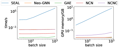
(a) Cora

(b) Citeseer

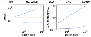
(c) Pubmed

(d) Ogbl-ppa

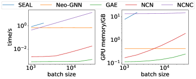
(e) Ogbl-ddi

(f) Ogbl-citation2

Figure 5: Inference time and GPU memory on datasets. The process we measure includes preprocessing, MPNN, and predicting one batch of test links.

Let $t$ denote the number of target links, $n$ denote the number of nodes in the graph, and $d$ denote the maximum node degree. Existing models’ time complexity can be expressed in $O(B+Ct)$, where $B,C$ are irrelevant to $t$. $B$ and $C$ of models are summarized in Table 5. The derivation of the time complexity is as follows. As NCN, GAE, and GNN with separated structural features run MPNN on the original graph, they share similar $B=ndF+nF^{2}$. Specifically, BUDDY (Chamberlain et al., 2022) uses a simplified MPNN with $B=ndF$. In contrast, $B$ of SEAL is $0$ as it does not run MPNN on the original graph. For each target link, vanilla GNN only needs to feed the feature vector to MLP for each link, so $C=F^{2}$. Besides GAE’s operation, BUDDY further needs to hash the structure for structural features, whose complexity is complex but higher than $d$, and Neo-GNN computes pairwise feature with $O(d^{l})$ complexity, where $l$ is the number of hop Neo-GNN consider. NCN needs to compute common neighbor: $O(d)$, pool node embeddings: $O(dF)$, and feed to MLP: $O(F^{2})$. NCNC-$1$ runs NCN for each potential common neighbor: $O(F^{2}+d(dF+F^{2}))=O(d^{2}F+dF^{2})$. Similarly, NCNC-$K$ runs $O(d)$ times NCNC-$(K\!-\!1)$, so its time complexity is $O(d^{K+1}F+d^{K}F^{2})$. For each target link, SEAL segregates a subgraph of size $O(d^{l^{\prime}})$ and runs MPNN on it, so $C=d^{l^{\prime}}F^{2}+d^{l^{\prime}+1}F$, where $l^{\prime}$ is the number of hops of the subgraph.

Appendix D Experimental Settings

Computing infrastructure.  We leverage Pytorch Geometric and Pytorch for model development. All experiments are conducted on an Nvidia 4090 GPU on a Linux server.

Baselines.  We directly use the results reported in (Chamberlain et al., 2022).

Model hyperparameter.  We use optuna to perform random searches. Hyperparameters were selected to maximize validation score. The best hyperparameters selected for each model can be found in our code.

Training process. We utilize Adam optimizer to optimize models and set an epoch upper bound $100$.

Appendix E Scalability Comparison on datasets

The time and memory consumption of models on different datasets are shown in Figure 5. On these datasets, we observe results similar to those on the ogbl-collab dataset in Section 6.2: NCN achieves similar computation overhead to GAE; NCNC usually scales better than Neo-GNN; SEAL’s scalabilty is the worst. However, on the ogbl-citation2 dataset, SEAL has the lowest GPU memory consumption with small batch sizes, because the whole graph in ogbl-citation2 is large, on which MPNN is expensive, while SEAL only runs MPNN on small subgraphs sampled from the whole graph, leading to lower overhead.

References

- Adamic & Adar (2003) Adamic, L. A. and Adar, E. Friends and neighbors on the web. Social networks, 25(3):211–230, 2003.
- Barabási & Albert (1999) Barabási, A.-L. and Albert, R. Emergence of scaling in random networks. science, 286(5439):509–512, 1999.
- Chamberlain et al. (2022) Chamberlain, B. P., Shirobokov, S., Rossi, E., Frasca, F., Markovich, T., Hammerla, N., Bronstein, M. M., and Hansmire, M. Graph neural networks for link prediction with subgraph sketching. CoRR, abs/2209.15486, 2022.
- Das et al. (2020) Das, R., Godbole, A., Monath, N., Zaheer, M., and McCallum, A. Probabilistic case-based reasoning for open-world knowledge graph completion. In Empirical Methods in Natural Language Processing, 2020.
- Gilmer et al. (2017) Gilmer, J., Schoenholz, S. S., Riley, P. F., Vinyals, O., and Dahl, G. E. Neural message passing for quantum chemistry. In International conference on machine learning, pp. 1263–1272, 2017.
- Hamilton et al. (2017) Hamilton, W. L., Ying, R., and Leskovec, J. Inductive representation learning on large graphs. Advances in Neural Information Processing Systems, pp. 1025–1035, 2017.
- Hu et al. (2020) Hu, W., Fey, M., Zitnik, M., Dong, Y., Ren, H., Liu, B., Catasta, M., and Leskovec, J. Open graph benchmark: Datasets for machine learning on graphs. In Advances in Neural Information Processing Systems, 2020.
- Judea (2009) Judea, P. Causality: Models, Reasoning, and Inference. Cambridge University Press, 2009.
- Kipf & Welling (2016) Kipf, T. N. and Welling, M. Variational graph auto-encoders. CoRR, abs/1611.07308, 2016.
- Kipf & Welling (2017) Kipf, T. N. and Welling, M. Semi-supervised classification with graph convolutional networks. In International Conference on Learning Representations, 2017.
- Liben-Nowell & Kleinberg (2003) Liben-Nowell, D. and Kleinberg, J. The link prediction problem for social networks. In Proceedings of the twelfth international conference on Information and knowledge management, pp. 556–559, 2003.
- Souri et al. (2022) Souri, E. A., Laddach, R., Karagiannis, S. N., Papageorgiou, L. G., and Tsoka, S. Novel drug-target interactions via link prediction and network embedding. BMC Bioinform., 23(1):121, 2022.
- Xu et al. (2019) Xu, K., Hu, W., Leskovec, J., and Jegelka, S. How powerful are graph neural networks? In International Conference on Learning Representations, 2019.
- Yang et al. (2022) Yang, H., Lin, Z., and Zhang, M. Rethinking knowledge graph evaluation under the open-world assumption. pp. 13683–13694, 2022.
- Yang et al. (2016) Yang, Z., Cohen, W. W., and Salakhutdinov, R. Revisiting semi-supervised learning with graph embeddings. In Proceedings of the 33nd International Conference on Machine Learning, volume 48, pp. 40–48, 2016.
- Yun et al. (2021) Yun, S., Kim, S., Lee, J., Kang, J., and Kim, H. J. Neo-gnns: Neighborhood overlap-aware graph neural networks for link prediction. In Advances in Neural Information Processing Systems, pp. 13683–13694, 2021.
- Zhang & Chen (2018) Zhang, M. and Chen, Y. Link prediction based on graph neural networks. Advances in Neural Information Processing Systems, 31:5165–5175, 2018.
- Zhang & Chen (2020) Zhang, M. and Chen, Y. Inductive matrix completion based on graph neural networks. In International Conference on Learning Representations, 2020.
- Zhang et al. (2021) Zhang, M., Li, P., Xia, Y., Wang, K., and Jin, L. Labeling trick: A theory of using graph neural networks for multi-node representation learning. Advances in Neural Information Processing Systems, 34:9061–9073, 2021.
- Zhou et al. (2009) Zhou, T., Lü, L., and Zhang, Y.-C. Predicting missing links via local information. The European Physical Journal B, 71(4):623–630, 2009.
- Zhu et al. (2021) Zhu, Z., Zhang, Z., Xhonneux, L. A. C., and Tang, J. Neural bellman-ford networks: A general graph neural network framework for link prediction. In Advances in Neural Information Processing Systems, pp. 29476–29490, 2021.