Abstract

We review applications of Yangain symmetry to high-energy QCD phenomenology. Some basic facts about high-energy QCD are recalled, in particular the spinor-helicity form of scattering amplitudes, the scale evolution equations of deep-inelastic scattering structure functions and the high-energy asymptotics of scattering. As the working tool the Yangian symmetric correlators are introduced and constructed in the framework of the Yangian algebra of $g\ell(n)$ type. We present the application to the tree scattering amplitudes and their iterative relation, to the parton splitting amplitudes and the kernels of the scale evolution equations of structure functions and to the equations describing the high-energy asymptotics of scattering.

keywords: Non-abelian gauge field theory, Quantum chromodynamics, scattering amplitudes, Bjorken asymptotics, Regge asymptotics, Yang-Baxter relations, Yangian algebra, Yangian symmetric correlators.

1 Gauge field theories and Quantum integrable systems

The history of Quantum integrable systems started with simple models for demonstrating basic physics, spin chains [1], scattering in one dimension [2], two-dimensional lattices [3]. In the first period the application to Quantum field theory was restricted to exceptional and sophisticated models in 1+1 dimensions.

The basic methodical concepts, Yang-Baxter relations, Bethe ansatz, established in the first basic publications, have been developed and extended to the Quantum inverse scattering method [4, 5, 6, 7, 8]. A new chapter of mathematics, the Quantum algebra, has been opened [9, 10], which is actively developing.

Quantum chromodynamics (QCD) is now well established as the gauge field theory of hadronic interactions, relying on basic concepts as non-abelian gauge field theory [11], its quantization [12, 13], renormalizability [14], asymptotic freedom [15, 16], and the quark model [17]. After the period of experimental confirmation the phenomenology of high-energy scattering is now oriented on finding signals beyond the Standard Model and on understanding the detailed structures of hadronic interaction, where extensive perturbative QCD calculations serve as a working tool.

The first application of Quantum integrable systems to high-energy QCD was pointed out by Lipatov [18]. Treating the Regge asympototics [19, 20, 21] in perturbative gauge theory [22, 23, 24] he showed that the multiple exchange of reggeized gluons can be treated as a Heisenberg quantum spin chain with the spin $\frac{1}{2}$ representations at its sites replaced by infinite-dimensional representations.

It was clear immediately, that the Bjorken asymptotics [25, 26, 27, 28, 29, 30] and the composite operator renormalization have similar features of integrability [31]. In both cases the Yangian symmetry underlying integrability is based on conformal symmetry, which is broken by loop corrections in the case of QCD. The breaking is suppressed by supersymmetry and is absent in $\mathcal{N}=4$ super Yang-Mills theory. Much work has been devoted in the last decades to super Yang-Mills theory under this aspect. Quantum integrability works in the composite operator renormalization in the planar limit to all orders [32] and in the computation of scattering amplitudes and Wilson loops [33, 34, 35].

Describing the relations of high-energy QCD to Yangian symmetry we do not intend to give a review of all relevant literature. Only a few references will be given. We try to include sufficient details of explanations in order to make the text readable without consulting these papers and books.

We shall recollect the subjects of high-energy QCD, scattering amplitudes in helicity form, Bjorken asymptotics and Regge asymptotics, where the applications are to be addressed. We shall formulate well-known relations, emphasizing the conformal symmetry, in order to prepare the comparison with the results of the Yangian symmetry. [36], [37] provide a broader introduction with a similar orientation.

We shall not attempt to give a complete introduction with general and rigorous definitions to the basics of Quantum algebra. For an introduction to the particular subject of Yangian algebra we refer to [38]. We focus on the items needed to define the Yangian symmetric correlators (YSC), to derive and to explain the relations used for their construction. We shall introduce the Yangian algebra notions in a way well understandable by physicists. The algebra generators are constructed from underlying Heisenberg algebra generators like in Quantum mechanics the operators of observables are constructed from the basic position and momentum operators.

Our approach uses in part ideas and methods developed for the the scattering amplitude computations, [35] Unlike the majority of related publications we do not approach the amplitudes directly and do not work in the frame of super Yang-Mills.

The YSC are obtained as N-point functions for Yangians of type $g\ell(n)$ in terms of expressions depending on $n$ and a set of parameters. In the applications $n$ will be specified to $4$ for amplitudes or to $2$ for evolution kernels of structure functions and for reggeon interaction kernels. The representation parameters are related in particular to homogeneity weights, which allow to describe the scattering states by substituting particular values. The dependence of the amplitudes or kernels on the particle type and helicity is derived from the analytic parameter dependence of the YSC by approaching particular values. The construction methods of YSC are related to the method of on-shell graphs in the amplititude construction [39]. In the original form of the latter method [35] no parameters appeared. In a number of papers the deformation of amplitude expressions by parameters has been studied and their eventual role for regularization of loop divergencies has been discussed [40, 41, 42, 43]. The parameters characterizing the monodromy defining the YSC play the essential role in our approach.

2 High-energy scattering in QCD

2.1 Scattering amplitudes

We shall consider the scattering amplitudes of quarks and gluons contributing to high-energy hadronic processes, e.g. inclusive jet production, $AB\to jet+X$, at large values of $s=(p_{A}+p_{B})^{2}$.

The advantages of using helicity states in the perturbative calculation of scattering amplitudes in gauge theories were known for long time [44] and widely used in the detailed calculations for collider phenomenology [45]. Both the momenta and the polarization states of the scattering quarks and gluons are expressed in terms of helicity spinors. The spinor components of massless momenta appear as products of the components of a left and right spinor,

$$k_{\alpha,\stackrel{{\scriptstyle\cdot}}{{\alpha}}}=\sigma_{\alpha,\stackrel{{\scriptstyle\cdot}}{{\alpha}}}^{\mu}k_{\mu}=\lambda_{\alpha}\bar{\lambda}_{\stackrel{{\scriptstyle\cdot}}{{\alpha}}}$$ (2.1)

The solutions of the massless Dirac equation can be expressed in terms of the Weyl spinors and they represent the helicity states of the scattering quark. The polarization vectors characterizing the helicity states of the gluons can be composed with the help of reference spinors $\mu_{\alpha},\bar{\mu}_{\stackrel{{\scriptstyle\cdot}}{{\alpha}}}$, the factors of the light-like gauge vector $q_{\alpha,\stackrel{{\scriptstyle\cdot}}{{\alpha}}}=\mu_{\alpha}\bar{\mu}_{\stackrel{{\scriptstyle\cdot}}{{\alpha}}}$.

$$\epsilon^{+}_{\alpha,\stackrel{{\scriptstyle\cdot}}{{\alpha}}}=\frac{\lambda_{\alpha}\bar{\mu}_{\stackrel{{\scriptstyle\cdot}}{{\alpha}}}}{[\bar{\mu}\bar{\lambda}]},\ \ \ \epsilon^{-}_{\alpha,\stackrel{{\scriptstyle\cdot}}{{\alpha}}}=\frac{\mu_{\alpha}\bar{\alpha}_{\stackrel{{\scriptstyle\cdot}}{{\alpha}}}}{<\mu\lambda>}.$$ (2.2)

The spinor indices $\alpha,\stackrel{{\scriptstyle\cdot}}{{\alpha}}$ take two values and the inner product of left-handed (undotted) spinors is abbreviated by angular brackets and the one of right-handed (dotted) by square brackets,

$$<\mu\lambda>=\mu_{1}\lambda_{2}-\mu_{2}\lambda_{1},\ \ \ [\bar{\mu}\bar{\lambda}]=\bar{\mu}_{1}\bar{\lambda}_{2}-\bar{\mu}_{2}\bar{\lambda}_{1}.$$ (2.3)

At high energies the massless case can be adopted as a first approximation, and then conformal symmetry holds at tree level. The action of infinitesimal conformal transformations, originally representing the actions on space-time coordinates, the shift $P_{\mu}$, the Lorentz $M_{\mu\nu}$, the special-conformal $K_{mu}$ and the dilatation $D$ transformations, appear in the spinor helicity representation as [46]

$$P_{\alpha,\stackrel{{\scriptstyle\cdot}}{{\alpha}}}=\lambda_{\alpha}\bar{\lambda}_{\stackrel{{\scriptstyle\cdot}}{{\alpha}}},\ \ M_{\alpha\beta}=\lambda_{\alpha}\partial_{\beta},\ \ \bar{M}_{\stackrel{{\scriptstyle\cdot}}{{\alpha}}\stackrel{{\scriptstyle\cdot}}{{\beta}}}=\bar{\lambda}_{\stackrel{{\scriptstyle\cdot}}{{\alpha}}}\bar{\partial}_{\stackrel{{\scriptstyle\cdot}}{{\beta}}},$$

$$K_{\alpha,\stackrel{{\scriptstyle\cdot}}{{\alpha}}}=\partial_{\alpha}\bar{\partial}_{\stackrel{{\scriptstyle\cdot}}{{\alpha}}},\ \ \ D=\frac{1}{2}(\lambda_{\alpha}\partial^{\alpha}+\bar{\lambda}_{\stackrel{{\scriptstyle\cdot}}{{\alpha}}}\bar{\partial}^{\stackrel{{\scriptstyle\cdot}}{{\alpha}}}+2).$$ (2.4)

The Lorentz vector components are transformed into the spinor components as in the particular case of the momentum above (2.1).

The eigenvalues of the dilatation in action on $\epsilon^{\pm}_{\alpha,\stackrel{{\scriptstyle\cdot}}{{\alpha}}},\lambda_{\alpha},\bar{\lambda}_{\stackrel{{\scriptstyle\cdot}}{{\alpha}}}$ are the canonical scaling dimensions of the corresponding fields in the QCD action, namely $1$ or $\frac{3}{2}$ for gluons or quarks. (Here $D$ measures the momentum dimension as $+1$, $[D,P_{\alpha,\stackrel{{\scriptstyle\cdot}}{{\alpha}}}]=P_{\alpha,\stackrel{{\scriptstyle\cdot}}{{\alpha}}}$). The scattering states are characterized by the helicities, the eigenvalues of the helicity operator $\hat{h}$,

$$2\hat{h}=\bar{\lambda}_{\stackrel{{\scriptstyle\cdot}}{{\alpha}}}\bar{\partial}_{\stackrel{{\scriptstyle\cdot}}{{\alpha}}}-\lambda_{\alpha}\partial_{\alpha},$$ (2.5)

commuting wth all conformal transformations (2.4).

The spinor-helicity presentation of the conformal symmetry generators does not have the Jordan-Schwinger form. This form is obtained by elementary canonical transformations on the left spinor variables,

$$\begin{pmatrix}\partial_{\alpha}\\ \lambda_{\alpha}\end{pmatrix}\rightarrow\begin{pmatrix}x_{\alpha}\\ -\partial_{x\ \alpha}\end{pmatrix}.$$ (2.6)

The two canonical pairs of the right spinors are not changed, but we prefer to rename them as

$$\begin{pmatrix}\bar{\partial}_{\stackrel{{\scriptstyle\cdot}}{{\alpha}}}\\ \bar{\lambda}_{\stackrel{{\scriptstyle\cdot}}{{\alpha}}}\end{pmatrix}\rightarrow\begin{pmatrix}\partial_{x\ 2+\stackrel{{\scriptstyle\cdot}}{{\alpha}}}\\ x_{2+\stackrel{{\scriptstyle\cdot}}{{\alpha}}}\end{pmatrix}.$$ (2.7)

In terms of the resulting Witten twistor canonical pairs $x_{a},\partial_{a}$ the conformal symmetry generators are written in the Jordan-Schwinger form as

$$M_{ab}=x_{a}\partial_{b}.$$ (2.8)

The indices take 4 values, $a,b=1,...,4$. The helicity operator (2.5) is included as the trace of the $4\times 4$ matrix of generators.

$$2\hat{h}\to x_{1}\partial_{1}+x_{2}\partial_{2}+\partial_{3}x_{3}+\partial_{4}x_{4},\ \ \ 2\hat{h}=(x\partial)+2.$$ (2.9)

The momenta of the incoming particles $A\ B$ lead us to prefer in the center-of-mass frame the basis of light-like vectors $n_{+},n_{-},n_{*},n_{o}$,

$$p_{A}={\frac{\sqrt{s}}{2}}n_{+}+\mathcal{O}(\frac{M^{2}}{s}),\ \ \ p_{B}={\frac{\sqrt{s}}{2}}n_{-}+\mathcal{O}(\frac{M^{2}}{s}).$$ (2.10)

$n_{*},n_{o}$ span the transverse plane. The normalization is $n_{+}n_{-}=2,n_{*}n_{o}=-2$. A generic Lorentz vector $k$ is expanded as

$$k=k^{-}n_{-}+k^{+}n_{+}+\kappa n_{*}+\kappa^{*}n_{o}.$$ (2.11)

If it is light-like, $k^{+}k^{-}=\kappa\kappa^{*}$, then it can be factorised as in (2.1), $(\lambda)=(\lambda_{1},\lambda_{2}),(\bar{\lambda})=(\bar{\lambda}_{1},\bar{\lambda}_{2})$ with

$$(\lambda)=(\sqrt{k^{+}},\frac{\kappa}{\sqrt{k^{+}}}),\ \ \ (\bar{\lambda})=(\sqrt{k^{+}},\frac{\kappa^{*}}{\sqrt{k^{+}}}).$$ (2.12)

The polarisation vectors of a scattering gluons of momentum $k$ are

$$\epsilon^{+}(k)=\bar{E}(k)(\frac{n_{o}}{\sqrt{2}}+\frac{k^{-}}{\sqrt{2}\kappa^{*}}n_{-}),\ \ \epsilon^{-}(k)=E(k)(\frac{n_{*}}{\sqrt{2}}+\frac{k^{-}}{\sqrt{2}\kappa}n_{-})$$ (2.13)

with $n_{-}$ chosen as the gauge vector and $\bar{E}k)E(k)=1$. Their spinor form factorizes as written above (2.2), e.g.

$$\epsilon_{\alpha,\stackrel{{\scriptstyle\cdot}}{{\alpha}}}^{+}(k)=const\mu^{-}_{\alpha}\epsilon^{+}_{\stackrel{{\scriptstyle\cdot}}{{\alpha}}},\ \ (\mu)=(n_{+})=(1,0),\ \ (\epsilon^{+}(k))=E(k)(\frac{k^{-}}{\kappa^{*}},1)$$ (2.14)

A way to calculate the lowest order perturbative contributions starts from the light-cone gauge form of the action. Being aware of the peculiarities of this non-covariant form we see the advantage that the physical degrees of freedom of the scattering partons are described by the transverse components $A^{*},A$ of the gauge field potential and projections $f^{*},f$ of the fermion fields in the QCD action after imposing the gauge $n_{-}A=0$ and integrating in the path integral over the redundant components $n_{+}^{\mu}A_{\mu}$ and $n_{+}^{\mu}\gamma_{\mu}\psi$. Here we consider the Dirac fermion field $\psi$ decomposed with respect to a basis of Majorana spinors $u_{a,b},a=\pm,b=o,*$ obeying $\gamma^{\pm}u_{\pm,b}=0,\gamma^{*}u_{a,o}=\gamma^{o}u_{a,*}=0$, with the vector of the Dirac gamma matrices decomposed in analogy to the momentum vector (2.11). $f^{*},f$ represent the two helicities of a quark of particular chirality and flavor. The field degrees of freedom of the quarks and gluons are directly represented by the fields, $A^{*},A$, the gluons of helicities $+1,-1$, and $f^{*},f$, the quarks of a particular flavor and particular chirality of helicities $+\frac{1}{2},-\frac{1}{2}$.

We write the kinetic part of the resulting light cone action for later reference,

$$S_{2}=\int d^{4}y\mathcal{L}_{2}(y),\ \ \ \mathcal{L}_{2}(y)=-2A^{B*}(y)(\partial_{+}\partial_{-}-\partial\partial^{*})A^{B}(y)+if^{b*}\partial_{+}^{-1}(\partial_{+}\partial_{-}-\partial\partial^{*})f^{b}(y).$$ (2.15)

$b$ runs over the range of the fundamental gauge group representation $b=1,...,N_{c}$ and $B$ over the range of the adjoint representation, $B=1,...,N_{c}^{2}-1$ and $\partial_{\pm}=\frac{1}{2}(\partial_{0}\pm\partial_{3}),\ \ \partial^{*}=\frac{1}{2}(\partial_{1}+i\partial_{2})$.

The dependence of the amplitudes on the the gauge group (color ) indices can be separated [45]. Here we focus on the the amplitude factors carrying the dependence on momenta and helicities.

We label the parton scattering states by their helicities and assume that the position $I$ in the array of arguments stands for the corresponding momentum $k_{I}$ and helicity spinors $\lambda_{I},\bar{\lambda}_{I}$. We assume all momenta ingoing, unifying in this way amplitudes related by crossing. In the planar partial amplitudes the dependence on the scattering states is cyclic.

In the case of physical (on-shell) momentum values $\bar{\lambda}_{\stackrel{{\scriptstyle\cdot}}{{\alpha}}}$ is complex conjugated to $\lambda_{\alpha}$. In course of a calculation we allow for complex momentum values. In particular modifications of values depending on a complex parameter $c$, preserving the momentum conservation condition, can be considered. The analytic structure of the $c$ dependence of the amplitudes $M(c)$ is determined by the physical unitarity. Tree amplitudes result in meromorphic functions of $c$ and as a consequence one obtains the BCFW iteration relations [47].

Consider the $N$ particle helicity amplitude $M_{1,..,N}$ and deform the helicity variables as

$$\bar{\lambda}_{1}\to\bar{\lambda}_{1}-c\bar{\lambda}_{N},\lambda_{N}\to\lambda_{N}+c\lambda_{1}$$ (2.16)

and $k_{1}(c)=\lambda_{1}(\bar{\lambda}_{1}-c\bar{\lambda}_{N})$, $k_{N}(c)=(\lambda_{N}+c\lambda_{1})\bar{\lambda}_{N}$. The deformed amplitude $M_{1^{*},2,...,N^{*}}(c)$ has single poles at $c=c_{l}$ corresponding to the one-particle intermediate states, where

$$P_{l}(c)=P_{l}-c\lambda_{1}\bar{\lambda}_{N},P_{l}=k_{1}+...+k_{l}$$

is light-like, $P_{l}(c_{l})^{2}=0$. This leads to the BCFW interative relation

$$M_{1,..,N}=\sum_{l}\sum_{h}M^{h}_{1,...,l,P}(c_{l})\frac{1}{P_{l}^{2}}M^{-h}_{P_{l},l+1,...,N}(c_{l}).$$

$M^{h}_{1,...,l,P}(c_{l})$ is the tree amplitude of $l+1$ particles of momenta $k_{1}(z_{l}),k_{2},...,k_{l},P_{l}(c_{l})$ and $h$ is the helicity of the last one. $M^{-h}_{P_{l},l+1,...,N}(z_{l})$ is the tree amplitude of $N-l+1$ particles with momenta $-P_{l}(c_{l}),k_{l+1},...,k_{N}(c_{l})$ and helicity $-h$ of the first one. Here it is assumed that the deformed amplitude vanishes at $c\to\infty$, which holds e.g. in the gluon case for helicity values $-1$ for particle 1 and $+1$ for particle $N$.

The deformation (2.16) can be written by shift operators as

$$M_{1,...,N}(c)=e^{-c\bar{\lambda}_{N}\bar{\partial}_{1}}e^{c\lambda_{1}\partial_{N}}M_{1,...,N},\ \ \ \ \bar{\partial}_{1}^{\stackrel{{\scriptstyle\cdot}}{{\alpha}}}=\frac{\partial}{\partial\bar{\lambda}_{1\stackrel{{\scriptstyle\cdot}}{{\alpha}}}},\partial_{N}^{\alpha}=\frac{\partial}{\partial\lambda_{N\alpha}},$$

and in terms of the amplitudes with energy-momentum delta included, $\widetilde{M}_{1,...,l}=M_{1,...,l}\delta(\lambda_{1\alpha_{1}}\bar{\lambda}_{1,\stackrel{{\scriptstyle\cdot}}{{\alpha}}_{1}}+...+\lambda_{l\alpha_{l}}\bar{\lambda}_{l,\stackrel{{\scriptstyle\cdot}}{{\alpha}}_{l}})$, the particular contribution to $\widetilde{M}_{1,...,N}$ of the channel $1,..,l\to l+1,...,N$ obtains the form

$$\int_{\mathcal{C}_{l}}\frac{dc}{c}\exp({-c\bar{\lambda}_{N\stackrel{{\scriptstyle\cdot}}{{\alpha}}}\bar{\partial}_{1}^{\stackrel{{\scriptstyle\cdot}}{{\alpha}}}})\exp({c\lambda_{1\alpha}\partial_{N}^{\alpha}})\int d^{4}P\delta(P^{2})\widetilde{M}^{h}_{1,...,l,P}\widetilde{M}^{-h}_{P,l+1,...,N}.$$ (2.17)

$\mathcal{C}_{l}$ denotes the small circle around $c_{l}$.

The 3-point amplitudes can be used as the building blocks to construct all tree amplitudes. In the Parke-Taylor form [48] we have e.g.

$$M(-1,-1,+1)=\frac{<12>^{4}}{<12><23><31>},\ \ \ M(-\frac{1}{2}.-1,+\frac{1}{2})=\frac{<12>^{3}<23>}{<12><23><31>}.$$

The amplitudes with all helicities $h_{i}$ reversed are obtained by replacing the brackets $<...>$ by $[...]$ (2.3 ). Further 3-point amplitudes are obtained from the above by cyclicity, the remaining ones vanish. All cases can be summarized as

$$M(h_{1},h_{2},h_{2})=<12>^{2\eta h_{3}+1}<23>^{2\eta h_{1}+1}<31>^{2\eta h_{2}+1},\ \ \ h_{1}+h_{2}+h_{3}=\eta,\eta=\pm 1.$$ (2.18)

2.2 The Bjorken asymptotics

Deep-inelastic electron - proton scattering $eP\to eX$ ($X$ denotes multi-hadron states ) is the prominent example of processes described by the Bjorken asymptotics of QCD. The electron scatters at large momentum transfer $q$, $-q^{2}=Q^{2}\gg M^{2}$. The data on this process allow to resolve the structure of the hadron $P$ into quasi-free quarks and gluons [25]. This heuristic view is confirmed by the analysis of the relevant Feynman graphs in the leading $\ln Q^{2}$ approximation [26, 27, 28].

The inclusive cross section factorizes into the leptonic and hadronic tensor factors. The latter can be considered as the s-channel discontinuity of the virtual Compton scattering amplitude, $\gamma^{*}P\to\gamma^{*}P$. It expands into Lorentz structures multiplied by structure functions $F(z,Q^{2}),z=\frac{Q^{2}}{2(pq)}$.

In the perturbative expansion of the hadronic tensor we see (Fig. 1 ) the virtual Compton scattering off a quark convoluted with the structure function of the hadron $F(z,Q^{2})$. The Bjorken variable $z=\frac{Q^{2}}{2(pq)}$ is the fraction of the proton momentum $p$ carried by the quark and $F(z,Q^{2})$ can be interpreted as the probability distribution for finding in the target the particular parton with momentum fraction $z$.

Figure 1: Virtual Compton scattering, contribution of the structure function F.

The asymptotics is governed by the Feynman graphs contributing a factor $\ln Q^{2}$ with each loop, i.e. the leading logarithmic approximation applies. In the light cone gauge the leading graphs simplify to ladders with self-energy and vertex corrections inserted. The leading contribution arises from the integration region of the loop momenta $k_{i}=k^{-}_{i}n_{-}+k^{+}_{i}n_{+}+\underline{\kappa}_{i}$ of strongly ordered transverse components

$$Q^{2}\gg\kappa_{N}^{2}\gg...\gg\kappa_{1}^{2}\gg M^{2}.$$ (2.19)

The loop integral reduces to the one over $k^{+}_{i}$, proportional to the momentum fraction of the proton, and the integration over the remaining components reduces to $\int\frac{d^{2}\kappa}{\kappa^{2}}$ to produce the required factor $\ln Q^{2}$.

The ladder rungs represent the partons hadronizing to the final hadronic state X. The sum of ladder contributions to the structure function leads to the equation for the structure function [26, 30, 29].

The elementary building block of the ladder is reduced in the limit (2.19) to the 4-point function $W_{ABCD}$ depending on the $k^{+}$ momentum components only, $k^{+}=\frac{2}{\sqrt{s}}z$. The sum of the leading ladder contributions including the self-energy and vertex corrections leads to the equation for the scale dependence of the structure function. $A,B,C,D$ denote the parton type and helicity ($\pm 1$ for gluons, $\pm\frac{1}{2}$ for quarks or anti-quarks). In the case of deep inelastic scattering $B$ is related to $A$ and also $C$ to $D$ by conjugation, $W_{A,\bar{A};C,\bar{C}}\to W_{A;C}$.

$$\frac{d}{d\xi}F_{A}(z;Q^{2})=-W_{A}F_{A}(z;Q^{2})+\sum_{C}\int_{z}^{1}\frac{dz^{\prime}}{z^{\prime}}W_{C,A}(\frac{z}{z^{\prime}})F_{C}(z^{\prime},Q^{2}).$$ (2.20)

The scale dependence is formulated in terms of $\xi(Q^{2})=-\frac{2N_{C}}{b}\ln\frac{\alpha(Q^{2})}{\alpha(M^{2})},$ depending on the one-loop QCD coupling $\alpha(Q^{2})=\frac{\alpha(M^{2})}{1+b\frac{\alpha(M^{2})}{2\pi}\ln\frac{Q^{2}}{M^{2}}},b=\frac{11}{3}N_{C}-\frac{2}{3}N_{F}$. $N_{c}$ stands for the number of colors and $N_{F}$ for the number of quark flavors .

This form is the one of a branching process with $W_{A,B}(z)$ being the rate of the parton $A$ to decay into a parton $B$ carrying the momentum fraction $z$ of $A$ and

$$W_{A}=\sum_{B}\int_{0}^{1}dzzW_{BA}(z).$$

The structure function $F_{A}(z;Q^{2})$ is proportional to the density of partons $A$ in the target hadron. Actually $W_{A,B}(z)$ is singular at $z=1$ and correspondingly $W_{A}$, and this branching picture becomes meaningful with a regularization at $z=1$ only.

With the definition of the evolution kernel as the well-defined distribution

$$P_{BA}(z)=W_{B,A}(z)-\delta_{A,B}\delta(1-z)W_{A}$$ (2.21)

we have the Altarelli-Parisi form [29],

$$\frac{d}{d\xi}F_{A}(z;Q^{2})=\sum_{C}\int_{z}^{1}\frac{dz^{\prime}}{z^{\prime}}P_{C,A}(\frac{z}{z^{\prime}})F_{C}(z^{\prime},Q^{2}).$$ (2.22)

It describes the scale $Q^{2}$ dependence of the structure functions and is usually referred to as DGLAP evolution equation.

The spectra of the operators defined by such kernels are obtained by calculating the moments

$$\gamma_{AB}(n)=\int_{0}^{1}dzz^{n-1}P_{AB}(z)$$ (2.23)

and diagonalizing the resulting matrices in the parton type indices $A,B$.

The hadronic tensor factor can be formulated also as the hadron states matrix element of the product of electromagnetic currents,

$$\int d^{4}xe^{iqx}<P^{\prime}|Tj_{\mu}(0)j_{\nu}(x)|P>.$$ (2.24)

$T$ stands for time-ordering. The treatment of the scale dependence can be formulated in terms of the operator product expansion and renormalization group [51, 52].

In the case at hand both hadron states coincide, the general case appears in semi-exclusive hard processes. In the general case in the Lorentz expansion of the hadronic tensor factor more structures contribute and the $n_{+}$ component of the momentum transfer appears as an additional variable in the structure functions, called generalized parton distributions [53, 54, 55, 56].

We see in both formulations of the hadronic tensor factor described that at the asymptotics the dynamics becomes one-dimensional. In the operator product form (2.24) the dominant integration region is $x^{2}\sim\frac{1}{Q^{2}}$. The leading contributions in the operator product expansion are products of two light cone components of quarks ($f^{*}(x),f(x)$) or gluons ($A^{*},A$) located at the light ray. Let us write such quasi-parton operator contributions as

$$F_{AB}(x_{1},x_{2};Q^{2})=<P^{\prime}|f^{*}_{A}(x_{1})f_{B}(x_{2})|P>,$$ (2.25)

where$A,B$ denote the parton type and helicity ($\pm 1$ for gluons, $\pm\frac{1}{2}$ for quarks or anti-quarks) and $x_{1},x_{2}$ are points on the light ray. The angular brackets stand for hadronic states.

For the field modes producing the leading contributions the QCD light cone action reduces to an one-dimensional effective action. In particular from the kinetic terms (2.15) we get schematically

$$S_{2Bj}=\int d^{1}x\mathcal{L}_{2Bj},\ \ \mathcal{L}_{2Bj}=2A^{*}A+if^{*}\partial^{-1}f.$$ (2.26)

The scaling dimensions of the effective parton fields are $\ell=-\frac{1}{2}$ for gluons and $\ell=-1$ for quarks.

By renormalization group the operator product contributions depend on momentum scale as

$$\frac{d}{d\xi}F_{AB}(x_{1},x_{2};Q^{2})=-\frac{1}{2}(W_{A}+W_{B})\delta_{AC}\delta_{BD}\delta(x_{1}-x_{1}^{\prime})\delta(x_{2}-x_{2}^{\prime})+$$ (2.27)

$$\sum_{CD}\int dx_{1}^{\prime}dx_{2}^{\prime}W_{CD,AB}(x_{1}^{\prime},x_{2}^{\prime};x_{1},x_{2})F_{CD}(x_{1}^{\prime},x_{2}^{\prime};Q^{2})$$

The evolution equation (2.20) is the light-cone momentum representation of the latter equation restricted to the case of vanishing momentum transfer. The position form is well suited for the case of generalized parton distributions. The eigenvalues of the operators defined by the kernels in light-cone position (2.27) and momentum representation (2.20), (2.22) coincide. The eigenvalues are the anomalous scaling dimensions of the corresponding linear combinations of local operator products obtained by expansion of the bi-local operators of (2.25) in powers of the positions $x_{1},x_{2}$.

The dynamics reduced in the Bjorken asymptotics to one dimension preserves the conformal symmetry at the tree level. The only relevant momentum component $k^{+}$ can be written as factorised into one-component variables, in analogy to the two-component spinor representation of light-like Lorentz vectors, $k^{+}=\lambda\bar{\lambda}$. The second spinor components (2.12) vanish with the transverse momenta in the asymptotics, the collinear limit.

The basic QCD three-point amplitudes (2.18) result in this limit in the parton splitting amplitudes $M_{{split}}$ [57]. They lead to the kernels $W_{AB}$ in analogy to the construction of the scattering amplitudes from the basic three-point amplitudes.

Consider the spinors (2.12) in terms of light-cone momentum components (2.11), substitute $k^{+}=\frac{\sqrt{s}}{2}z$ and choose $z_{1}=1,\kappa_{1}=0,z_{2}=z,\kappa_{2}=\kappa,z_{3}=1-z,\kappa_{3}=-\kappa$. The parton splitting amplitude $1\to 2+3$ is then

$$\lim_{\kappa\to 0}\frac{1}{<23>}M(h_{1},h_{2},h_{3})=\frac{z^{\frac{1}{2}}(1-z)^{\frac{1}{2}}}{z^{\eta h_{2}}(1-z)^{\eta h_{2}}}.$$

We obtain the symmetric from of the parton splitting amplitude, $z_{i}=\frac{2}{\sqrt{s}}k^{+}_{i},\sum z_{1}+z_{2}+z_{3}=0$, $h_{1}+h_{2}+h_{3}=\eta$,

$$M_{{split}}(z_{1},z_{2},z_{3};h_{1},h_{2},h_{3})=z_{1}^{\frac{1}{2}-\eta h_{1}}z_{2}^{+\frac{1}{2}-\eta h_{2}}z_{3}^{\frac{1}{2}-\eta h_{3}}.$$ (2.28)

The splitting amplitude results in the kernels of the above scale evolution equation as (changing here from the convention of ingoing momenta to the normal physical one)

$$W_{AB}(z)=\sum_{C}W_{ABC}(z),\ \ W_{ABC}(z)=|M_{split}(1,-z,z-1,h_{A},-h_{B}-h_{C})|^{2}.$$ (2.29)

We describe the action of the conformal symmetry in the Bjorken limit. Consider as generators $M_{ab}=x_{a}\partial_{b}$ (2.8), but now with the indices restricted to $a,b,=1,2$ and also the analogy of the elementary canonical transformation (2.6), (2.7) to the helicity form . Now $\alpha,\stackrel{{\scriptstyle\cdot}}{{\alpha}}$ take only one value so that the indices will be omitted. We have here (compare (2.9) )

$$2\hat{h}=(\underline{x}\underline{\partial})+1,\ \ (\underline{x}\underline{\partial})=x_{a}\partial_{a}.$$

Let the generators, $M_{ab}=x_{a}\partial_{b}$, act on functions of $x_{a}$. This representation is reducible to homogeneous functions of degree $2\ell$, $\phi(x)(x_{2})^{2\ell},\ \ x=\frac{x_{1}}{x_{2}}$. $2\ell$ is the eigenvalue of the dilatation $(\underline{x}\underline{\partial})$, and is related to the helicity as

$$2h=2\ell+1,$$ (2.30)

and the conformal symmetry generators act on $\phi(x)$ as

$$(M_{ab})=\begin{pmatrix}x\partial+\ell&\partial\\ -x(x\partial+2\ell)&x\partial-\ell\end{pmatrix}.$$ (2.31)

For $2\ell=0$ the Möbius transformations on the line parametrized by $x$ are generated.

This ratio variable $x$ is the one to represent the light-ray positions appearing above in the operator products and $k=\lambda\bar{\lambda}$ is to represent the light-cone momenta.

2.3 The Regge asymptotics

The Regge asymptotics of the scattering $AB\to A^{\prime}B^{\prime}$ is approached in the kinematics $s\gg t$, where $s=(p_{A}+p_{B})^{2},t=(p_{A}-p_{A^{\prime}})^{2}=q^{2}$. Tree amplitudes with charges and (physical) helicities of $A$ and $B$ coinciding with the ones of $A^{\prime}$ and $B^{\prime}$, correspondingly, have a leading contribution behaving as $s$, where gluons are exchanged in the $t$ channel. Amplitudes with $n_{q}$ quarks exchanged behave asymptotically as $s^{1-\frac{1}{2}n_{q}}$.

It is convenient to consider the Mellin transform of the amplitude,

$$M(s,t)=\int_{-i\infty+\delta}^{+i\infty+\delta}d\omega F(\omega,q)\left(\frac{s}{M^{2}}\right)^{1+\omega}.$$ (2.32)

Here the details about signature are suppressed. The Mellin amplitude $F(\omega,q)$, also called partial wave, appears as a convolution by integration over transverse momenta $\kappa_{i}$ of impact factors $\Phi_{A}(\underline{\kappa})$, coupling to the particles $A$ and $A^{\prime}$, and $\Phi_{B}(\underline{\kappa}^{\prime},)$, coupling to the particles $B$ and $B^{\prime}$, with the reggeon Green function $G(\omega,\underline{\kappa},\underline{\kappa}^{\prime})$, illustrated schematically in Fig. 2,

$$F(\omega,q)=\int d\underline{\kappa}d\underline{\kappa}^{\prime}\Phi_{A}(\underline{\kappa})G(\omega,\underline{\kappa},\underline{\kappa}^{\prime})\Phi_{B}(\underline{\kappa}^{\prime})$$ (2.33)

Actually there is a sum over contributions of multiple reggeon exchanges and $\underline{\kappa}$ stands for the set of reggeon transverse momenta. We shall use also the convolution with one of the impact factors, in the case of two reggeons

$$f(\omega,\kappa_{1},\kappa_{2})=\int d\kappa_{1}^{\prime}d\kappa_{2}^{\prime}G(\omega,\kappa_{1},\kappa_{2},\kappa_{1}^{\prime},\kappa_{2}^{\prime})\Phi_{B}(\kappa_{1}^{\prime},\kappa_{2}^{\prime}).$$

Figure 2: Mellin amplitude.

The asymptotics in $s$ is determined by the right-most singularities in $\omega$ of the reggeon Green functions $G(\omega,\underline{\kappa},\underline{\kappa}^{\prime})$ .

The reggeon Green functions corresponding to the single gluon or quark exchange are, correspondingly,

$$\frac{1}{|\kappa|^{2}}\frac{1}{\omega},\ \ \ \ \frac{1}{\kappa}\frac{1}{\omega+\frac{1}{2}},$$ (2.34)

or the complex conjugate for the opposite quark helicity. The transverse momentum dependence can be described by the propagators of the effective reggeon fields in two transverse dimensions,

$$S_{2R}=\int d^{2}x\mathcal{L}_{2R}(x),\ \ \mathcal{L}_{2R}(x)=-\mathcal{A}_{+}(x)\partial\partial^{*}\mathcal{A}_{-}(x)-\chi_{+}(x)\partial\chi_{-}(x)-\widetilde{\chi}_{+}(x)\partial\widetilde{\chi}_{-}(x).$$ (2.35)

The reggeon fields with subcript $+$ are to couple to the impact factor $\Phi_{A}$ and to particles flying almost in the direction $p_{A}$ and the fields with subscript $-$ are to couple to particles flying almost in the direction $p_{B}$.

In the leading logarithmic approximation the conformal symmetry is preserved, acting by linear fractions (Möbius transformations) on the transverse positions, separately for $x$ and $x^{*}$. We have in particular scale symmetry $x\to\lambda x,x^{*}\to\bar{\lambda}x^{*}$ for the corresponding transformation of the fields as appearing in the kinetic terms (2.35) with the scale exponents $(\ell,\bar{\ell})$ being $(0,0)$ for gluons and $(0,-\frac{1}{2})$ or $(-\frac{1}{2},0)$ for quarks.

In the leading logarithmic approximation the Feynman graph contributions proportional to $\ln s$ for each loop are summed. In the light-cone gauge the leading graphs simplify to ladders with the t-channel exchanged gluons or quarks being reggeized by loop corrections. The kinematics of the leading ladder contributions are characterized by the strong ordering conditions on the loop momentum components $k^{+},k^{-}$,

$$k^{+}_{1}\gg...\gg k^{+}_{N},\ \ \ k^{-}_{1}\ll...\ll k^{-}_{N}.$$ (2.36)

The integration over these components reduces to the logarithmic form $\sim\int\frac{dk^{+}}{k^{+}}$ and, consequently, the dynamics reduces to the two transverse dimensions.

The elementary building block of the ladder and the reggeization can be understood in terms of the effective production vertex [82]. Consider the scattering of two partons with production of a parton. The sum of the bremsstrahlung off the scattered parton Fig. 3a and the emission from the exchanged reggeon Fig. 3b is represented by the emission with the effective production vertex $V_{gg}$ Fig. 3c.

Figure 3: $2\to 3$ scattering. a) Bremsstrahlung, b) Direct emission, c) Effective production vertex.

For the gluonic reggeons we have in transverse momenta written in complex numbers the effective production vertex

$$V_{gg}(\kappa,\kappa^{\prime})=\frac{\kappa^{*}\kappa^{\prime}}{\kappa-\kappa^{\prime}}$$ (2.37)

or as an effective action term to be added to (2.35)

$$\mathcal{L}_{p}(x)=g(\partial\mathcal{A}_{+}(x)\partial^{*}\mathcal{A}_{-}(x))a(x).$$

$a(x)$ stands for the emitted gluon. Its momentum range is close to the mass shell. $\mathcal{A}_{\pm}$ are the exchanged gluonic reggeons with momenta in the range $k^{+}k^{-}\ll\kappa\kappa^{*}$.

Instead of the argument in terms of graphs Fig. 3 the effective production term can be obtained by integrating out (elimination by equation of motion) the modes far off shell, $k^{+}k^{-}\gg\kappa\kappa^{*}$, represented by the fat line in Fig. 3a.

The contribution of the elementary building block of the ladder Fig. 4a is obtained from this effective production vertex (black dot in the figure) as

$$K^{(0)}(\kappa_{1},\kappa_{2},\kappa_{1}^{\prime},\kappa_{2}^{\prime})=V_{gg}(\kappa_{1},\kappa^{\prime}_{1})V^{*}_{gg}(\kappa_{2},\kappa^{\prime}_{2})+c.c.$$ (2.38)

The one-loop contribution to the gluon reggeisation can be written as

$$\omega_{g}(\kappa)=\frac{1}{2(2\pi)^{3}}|\kappa|^{2}\int\frac{d^{2}\kappa^{\prime}}{|\kappa^{\prime}|^{2}|\kappa-\kappa^{\prime}|^{2}}.$$ (2.39)

Including this contribution modifies the Green function of the reggeized gluon from (2.34) to

$$\frac{1}{|\kappa|^{2}}\ \frac{1}{\omega+g_{r}^{2}\omega_{g}(\kappa)},\ \ \ g_{r}^{2}=\frac{g^{2}N_{c}}{2(2\pi)^{3}}.$$ (2.40)

The Green function of two non-interacting reggeised gluons is

$$G^{(0)}(\omega,\kappa_{1},\kappa_{2},\kappa_{1}^{\prime},\kappa_{2}^{\prime})=|\kappa_{1}|^{-2}|\kappa_{2}|^{-2}\delta(\kappa_{1}-\kappa_{1}^{\prime})\delta(\kappa_{2}-\kappa_{2}^{\prime})f^{(0)}(\omega,\kappa_{1},\kappa_{2}),$$

$$f^{(0)}(\omega,\kappa_{1},\kappa_{2})=\frac{1}{\omega+g_{r}^{2}\omega_{g}(\kappa_{1})+g_{r}^{2}\omega_{g}(\kappa_{2})}$$

The sum of the ladder graph contributions of the two-reggeon interaction is obtained by solving the equation

$$G(\omega,\kappa_{1},\kappa_{2},\kappa_{1}^{\prime},\kappa_{2}^{\prime})=G^{(0)}(\omega,\kappa_{1},\kappa_{2},\kappa_{1}^{\prime},\kappa_{2}^{\prime})+g_{r}^{2}\int\frac{d^{2}\kappa_{1}^{\prime}d^{2}\kappa_{2}^{\prime\prime}}{|\kappa_{1}^{\prime\prime}|^{2}|\kappa_{2}^{\prime\prime}|^{2}}K^{(0)}(\kappa_{1}^{\prime\prime},\kappa_{2}^{\prime\prime},\kappa_{1},\kappa_{2})G(\omega,\kappa_{1}^{\prime\prime},\kappa_{2}^{\prime\prime},\kappa_{1}^{\prime},\kappa_{2}^{\prime}).$$

The reggeization contribution $\omega_{g}(\kappa)$ (2.39) becomes well defined with regularization only and the bare kernel $K^{(0)}$ defines an operator only with regularization. We rewrite the equation in terms of the BFKL kernel resulting in a well defined operator at vanishing regularization parameter [22, 23, 24],

$$K(\kappa_{1}^{\prime},\kappa_{2}^{\prime},\kappa_{1},\kappa_{2})=K^{(0)}(\kappa_{1}^{\prime},\kappa_{2}^{\prime},\kappa_{1},\kappa_{2})-(\omega_{g}(\kappa_{1})+\omega_{g}(\kappa_{2}))\delta(\kappa_{1}-\kappa_{1}^{\prime})\delta(\kappa_{2}-\kappa_{2}^{\prime}),$$

$$\omega f(\omega,\kappa_{1},\kappa_{2})=g_{r}^{2}\int\frac{d^{2}\kappa_{1}^{\prime}d^{2}\kappa_{2}^{\prime}}{|\kappa_{1}^{\prime}|^{2}|\kappa_{2}^{\prime}|^{2}}K(\kappa_{1}^{\prime},\kappa_{2}^{\prime},\kappa_{1},\kappa_{2})f(\omega,\kappa_{1}^{\prime},\kappa_{2}^{\prime}).$$ (2.41)

The kernel can be reconstructed from elementary reggeon triple vertices [80], obtained from the transverse part of the induced vertex obtained from the bremsstrahlung contribution Fig. 3a. $\mathcal{V}^{+--}(\kappa_{1},\kappa_{2})$ is the interaction vertex of a reggeon $\mathcal{A}_{+}$ with two reggeons $\mathcal{A}_{-}$, $\kappa_{1},\kappa_{2}$ are the momenta of the latter.

$$\mathcal{V}^{-++}(\kappa_{1},\kappa_{2})=\mathcal{V}^{+--}(\kappa_{1},\kappa_{2})=|\kappa_{1}+\kappa_{2}|^{2}.$$ (2.42)

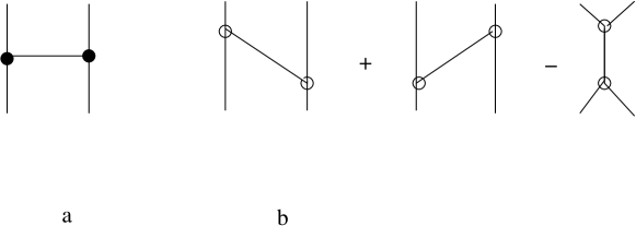
Figure 4: Elementary ladder block, composed by effective production vertices (a) or by reggeon triple vertices (b).

Fig. 4b shows the graphs with these vertices resulting in the bare BFKL kernel $K^{(0)}$ (2.38)), standing term by term for

$$\frac{|\kappa_{2}|^{2}|\kappa_{1}^{\prime}|^{2}}{|\kappa_{1}-\kappa_{1}^{\prime}|^{2}}+\frac{|\kappa_{1}|^{2}|\kappa_{2}^{\prime}|^{2}}{|\kappa_{1}-\kappa_{1}^{\prime}|^{2}}-|\kappa_{1}+\kappa_{2}|^{2}=K^{(0)}(\kappa_{1}^{\prime},\kappa_{2}^{\prime},\kappa_{1},\kappa_{2}),$$ (2.43)

and Fig. 5 shows the loop resulting in the reggeization $\omega_{g}$ (2.39). In Fig. 4b and Fig. 5 the edges of a triple reggeon vertex (open circle) pointing upwards represent $\mathcal{A}_{-}$ and the edges pointing downwards represent $\mathcal{A}_{+}$.

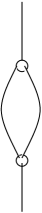
Figure 5: Reggeization loop composed of reggeon triple vertices.

The conformal symmetry of the equation (2.41) becomes evident after the transformation to transverse positions. The Fourier transformation is to be done with care because of divergencies. Schematically the result expressed as an operator in terms of the canonical pairs $x_{I},\partial_{I},I=1,2$ and their complex conjugates $x^{*}_{I},\partial^{*}_{I}$ can be understood applying to the expression of the BFKL kernel (2.41) the substitution rules

$$|\kappa_{1}-\kappa_{1}^{\prime}|\to-\ln|x_{12}|^{2},\omega(\kappa_{1})\to\psi(1)-\ln(\partial_{1}\partial_{1}^{*}),\ \ \kappa_{1}\to\partial_{1}^{*},\ \kappa_{2}^{*}\to\partial_{2}.$$ (2.44)

This leads to the equation for the Fourier transform $\widetilde{f}(\omega,x_{1},x_{2})$

$$\omega\widetilde{f}(\omega,x_{1},x_{2})=\frac{g^{2}N_{c}}{8\pi^{2}}\hat{H}_{g}\ \widetilde{f}(\omega,x_{1},x_{2})$$ (2.45)

with the BFKL hamiltonian $\hat{H}_{g}$ decomposing into a holomorphic and an anti-holomrophic parts, the first involving $x_{I},\partial_{I},I=1,2$ only and the second $x^{*}_{I},\partial^{*}_{I},I=1,2$ only.

$$\hat{H}_{g}=(H_{g}+H^{*}_{g}),$$

$$H_{g}=2\psi(1)-\partial_{1}^{-1}\ln x_{12}\ \partial_{1}-\partial_{2}^{-1}\ln x_{12}\ \partial_{2}-\ln\partial_{1}-\ln\partial_{2}.$$ (2.46)

Further formal operator manipulations lead to the expression in terms of the tensor Casimir operator

$$C_{12}=(M^{(1)}+M^{(2)})_{ab}(M^{(1)}+M^{(2)})_{ba},$$ (2.47)

where $M^{(I)}_{ab}$ are the operators in the matrix elements of (2.31) with $x,\partial$ replaced by $x_{I},\partial_{I}$ and $\ell$ by $\ell_{I}$. The symmetry algebra consists of two copies of $g\ell(2)$, generated by $M_{ab}$ acting on $x$ but not on $x^{*}$ and $M^{*}_{ab}$ acting on $x^{*}$. Correspondingly we have two labels $(\ell,\bar{\ell})$ for the representations, $\ell$ referring to the first and $\bar{\ell}$ referring to the second.

In the case of two gluonic reggeons considered the representation parameters are $(\ell_{1},\bar{\ell}_{1}),(\ell_{2},\bar{\ell}_{2})=(0,0),(0,0)$. This corresponds to the above remark after (2.35) about the scale dimensions of the reggeon fields. The formulation generalizes to more than two reggeons and to the inclusions of fermionic reggeons. The latter are described by the representations $(-\frac{1}{2},0)$ or $(0,-\frac{1}{2})$ depending on helicity and chirality [81].

The colour-dipole model [58, 59, 60, 61] of high-energy scattering leads to the integral form of the Hamiltonian

$$\hat{H}_{g}\widetilde{f}(\omega,x_{1},x_{2})=\frac{1}{\pi}\int d^{2}x_{0}\frac{|x_{12}|^{2}}{|x_{10}|^{2}|x_{20}|^{2}}\left(\widetilde{f}(\omega,x_{1},x_{2})-\widetilde{f}(\omega,x_{1},x_{0})-\widetilde{f}(\omega,x_{0},x_{2})\right).$$ (2.48)

$\widetilde{f}(\omega,x_{1},x_{2})$ can be regarded as the Mellin transform of the dipole distribution with respect to their end-points in the transverse plane and the equation (2.45) describes its evolution with rapidity $Y\sim\ln s$.

We present the arguments of [62] leading to this form. By the formal operator relations

$$\partial\ln x\ \partial^{-1}=\ln x+x^{-1}\partial^{-1},\ \ x\ln\partial\ x^{-1}=\ln\partial-\partial^{-1}x^{-1}$$ (2.49)

the Hamiltonian (2.46) is rewritten as

$$\hat{H}_{g}=4\psi(1)-2\ln|x_{12}|^{2}-2|x_{12}|^{-2}\ln|\partial_{1}\partial_{2}|^{2}|x_{12}|^{2}.$$ (2.50)

Regularizing the kernel in (2.48) we have

$$\int\frac{d^{2}x_{0}}{\pi}\frac{|x_{12}|^{2}}{(|x_{10}|^{2}+\delta^{2})(|x_{20}|^{2}+\delta^{2})}=\int_{0}^{1}d\alpha\frac{|x_{12}|^{2}}{(\alpha(1-\alpha)|x_{12}|^{2}+\delta^{2}}=2\ln{\frac{|x_{12}|^{2}}{\delta^{2}}}+\mathcal{O}(\delta^{2})$$

$$-\int\frac{d^{2}x_{0}}{\pi}\frac{|x_{12}|^{2}}{(|x_{10}|^{2}+\delta^{2})(|x_{20}|^{2}+\delta^{2})}\widetilde{f}(\omega,x_{1},x_{0})=|x_{12}|^{2}(\ln(\delta^{2}|dd_{2}|^{2}-2\psi(1))|x_{12}|^{-2}\widetilde{f}(\omega,x_{1},x_{2})+\mathcal{O}(\delta^{2})$$

This shows that the integral operator (2.48) acts in the limit of vanishing $\delta$ as the operator (2.50).

The eigenvalues of the operator defined by the kernel $K(\kappa_{1}^{\prime},\kappa_{2}^{\prime},\kappa_{1}\kappa_{2})$ (2.41) are easily calculated in the transverse momentum form in the forward limit, $\kappa_{1}+\kappa_{2}=-\kappa_{1}^{\prime}-\kappa_{2}^{\prime}=0$. In this case the eigenfunctions are

$$E^{(n,\nu)}(\kappa)=|\kappa|^{\frac{1}{2}+i\nu}\left(\frac{\kappa^{*}}{|\kappa|}\right)^{n},$$

a basis of functions on the complex plane for integer $n$ and $\nu\in\hbox{\bbd R}^{1}$. The eigenvalues can be written as

$$\Omega_{g}(n,\nu)=\chi_{0}(m)+\chi_{0}(\bar{m}),\chi_{0}(m)=2\psi(1)-\psi(m)-\psi(1-m),$$ (2.51)

$$m=\frac{1}{2}+i\nu+\frac{1}{2}n,\ \ \bar{m}=\frac{1}{2}+i\nu-\frac{1}{2}n.$$

$\chi_{0}(m)$ is actually a function of $m(1-m)$, the eigenvalue of the Casimir operator (2.47). In the form of transverse positions the eigenfunctions are the conformal three-point functions.

$$E^{(n,\nu)}(x_{1},x_{2};x_{0})=E_{m}(x_{1},x_{2};x_{0})E_{\bar{m}}(x^{*}_{1},x^{*}_{2};x^{*}_{0}),$$ (2.52)

$$E_{m}(x_{1},x_{2};x_{0})=\left(\frac{x_{12}}{x_{10}x_{20}}\right)^{m},$$

obeying the completeness relation

$$\delta^{(2)}(x_{1}-x_{1}^{\prime})\delta^{(2)}(x_{2}-x_{2}^{\prime})=\int d^{2}x_{0}\int_{-\infty}^{+\infty}d\nu\sum_{n=-\infty}^{+\infty}$$

$$\frac{\nu^{2}+\frac{n^{2}}{4}}{\pi^{4}|x_{11^{\prime}}|^{2}x_{22^{\prime}}|^{2}}E^{(n,\nu)*}(x_{1},x_{2},x_{0})E^{(n,\nu)}(x^{\prime}_{1},x^{\prime}_{2},x_{0}).$$

The orthogonality relation expresses the fact that this basis is twofold over-complete [63].

The spectral properties are the basis for giving the above forms of the BFKL operator and the unconventional steps of transformations (2.44), (2.49) well defined meanings.

The renormalized coupling, depending on the scale $Q^{2}$, enters the Bjorken limit evolution equations at leading order. In the BFKL equation, describing the Regge asymptotics, the bare coupling enters at leading order. Its renormalization is included at next-to-leading order only [64],[65], [66].

For the region of overlap of both asymptotics combinations of both types of equations have to be considered, including the BFKL contributions as corrections to the DGLAP equation [69] or improving the BFKL equation by the renormalization group [63]. In the overlap region the contributions of muti-reggeon exchange become important. They can be described by non-linear terms to be included into the BFKL equation [67, 68]. In the dipole picture the multi-reggeon contributions appear as creation of more dipoles [60, 61]. In the ultimate asymptotics a regime of saturation emerges [70, 71] allowing the application of thermodynamic concepts. Characteristics of the thermodynamic limit of models directly related to the integrable spin chains, where the BFKL hamiltonian describes the pair interaction, have been proposed to be applied here [72, 73].

3 Yangian symmetry

3.1 Monodromy matrix operators and symmetric correlators

We start with the formulation of the $g\ell(n)$ Lie algebra relations as the fundamental Yang-Baxter relation

$$\mathcal{R}(u-v)(L(u)\otimes I)(I\otimes L(v))=(I\otimes L(v))(L(u)\otimes I)\mathcal{R}(u-v).$$ (3.1)

Here $\mathcal{R}(u-v)$ stands for Yang’s $R$ matrix. Its size is $n^{2}\times n^{2}$ in our case and composed of the unit matrix and the matrix representing the permutation of the factors in the tensor product of the $n$-dimensional fundamental representation spaces, $\mathcal{R}(u)=uI_{n^{2}\times n^{2}}+P$. The $L$ matrices are of size $n\times n$ and linear in the spectral parameter $u$, $L(u)=uI_{n\times n}+L$. $L_{ab},a,b,=1,...,n$ are the generators of the Lie algebra $g\ell(n)$. In index notation we have

$$L_{ab}(u)=u\delta_{ab}+L_{ab},\ \ \ \mathcal{R}^{a_{1}a_{2}}_{b_{1}b_{2}}(u)=u\delta^{a_{1}}_{b_{1}}\delta^{a_{2}}_{b_{2}}+\delta^{a_{1}}_{b_{2}}\delta^{a_{2}}_{b_{1}}.$$ (3.2)

The Yangian algebra can be introduced by the matrix operator $T(u)$ obeying the above Yang-Baxter relation (3.1) with $L(u)$ substituted by $T(u)$ and where now the dependence on $u$ is not restricted as above. Then the generators of the extended Yangian algebra [9], [38] appear in the expansion of $T(u)$ in inverse powers of $u$ and the extended Yangian algebra relations follow from the Yang-Baxter relation (3.1).

We shall deal with evaluations of the $g\ell(n)$ Yangian of finite order $N$ where $T(u)$ is constructed from the $L$ matrices in the way well know in the context of integrable models. Let the matrix elements of $L_{I}(u_{I})$ act on the representation space $V_{I}$ and consider the matrix product defining the monodromy matrix

$$T(u,\delta_{1},\dots,\delta_{N})=T(\mathbf{u})=L_{1}(u_{1})\cdots L_{N}(u_{N}),\quad u_{I}=u+\delta_{I},$$ (3.3)

acting on the tensor product $V_{1}\otimes\cdots\otimes V_{N}$.

We consider the case of representations by homogeneous functions of $\mathbf{x}_{I}=(x_{i,1},...,x_{I,n})$ and the weight $2\ell_{I}$ is the degree of homogeneity,

$$\psi(\mathbf{x}_{I})=x_{i,n}^{2\ell_{I}}\phi(\mathbf{x}^{\prime}_{I}),\ \ \ \mathbf{x}_{I}^{\prime}=(\frac{x_{I,1}}{x_{I,n}},...,\frac{x_{I,n-1}}{x_{I,n}}).$$ (3.4)

The elements of the tensor product $V_{1}\otimes\cdots\otimes V_{N}$ are functions of $N$ points in the $n$ dimensional space.

We consider the Lie algebra generators of the Jordan-Schwinger (JS) form,

$$L^{+}_{I,ab}=\partial_{I,a}x_{I,b},\ \ \ L^{-}_{I,ab}=-x_{I,a}\partial_{I,b},$$ (3.5)

built from $n$ canonical pairs $x_{I,a},\partial_{I,a}$ at each point $I$,

$$[\partial_{I,a},x_{J,b}]=\delta_{IJ}\delta_{ab}.$$ (3.6)

Notice that the elementary canonical transformation

$$\begin{pmatrix}x_{I,a}\\ \partial_{I,a}\end{pmatrix}\rightarrow\begin{pmatrix}\partial_{I,a}\\ -x_{I,a}\end{pmatrix}$$ (3.7)

transforms $L_{I}^{+}(u)$ into $L_{I}^{-}(u)$.

We have the matrix inversion relations (for any point $I$)

$$\left(\frac{L^{+}(u)}{u}\right)^{-1}=\frac{L^{+}(-u-1-(\underline{x}\underline{\partial}))}{-u-1-(\underline{x}\underline{\partial})},\ \ \ \left(\frac{L^{-}(u)}{u}\right)^{-1}=\frac{L^{-}(-u+1+(\underline{x}\underline{\partial}))}{-u+1+(\underline{x}\underline{\partial})},$$ (3.8)

where $(\underline{x}\underline{\partial})=\sum_{a=1}^{n}x_{a}\partial_{a}$.

The two forms of JS generators are also related by matrix transposition, $(L^{t})_{ab}=L_{ba}$,

$$(L^{+}(u))^{t}=-L^{-}(-u-1).$$ (3.9)

This transposition operation and the inversion act depending on ordering,

$$(L^{+}(u))^{t\ -1}=(L^{+}(u+n))^{-1\ t}.$$ (3.10)

Related to integrals over the positions $x_{a}$ we consider another transposition operation acting on the canonical pairs as

$$(x_{a})^{T}=x_{a},\ \ \partial_{a}^{T}=-\partial_{a},$$

leaving indices unchanged but reversing the order in products of such operators, similar to the matrix transposition, at the same point e.g. $(x_{I,a}\partial_{I,b}\partial_{J,c})^{T}=(\partial_{I,b})^{T}(x_{I,a})^{T}\partial_{J,c}^{T}$.

$$(L^{+}(u))^{T}=(L^{-}(u))^{t}=-L^{+}(-u-1),\ \ \ (\underline{x}\underline{\partial})^{T}=-n-(\underline{x}\underline{\partial}).$$ (3.11)

We intend to consider representations by functions of $x_{I,a}$ homogeneous at each point $I$ (3.4), i.e. we restrict to the subspace of fixed eigenvalues of the dilatation operators, $(\underline{x}_{I}\underline{\partial}_{I})\to 2\ell_{I}$. The corresponding projector will be denoted by $\Pi_{I}(2\ell_{I})$.

The projection of the $L$ operator depends on this degree of homogeneity,

$$\Pi_{I}(2\ell_{I})L_{I}^{+}(u)\Pi_{I}(2\ell_{I})=L_{I}^{+}(u_{I}^{+},u_{I}),\ u_{I}^{+}=u+\delta_{I}+2\ell_{I}$$ (3.12)

The action of the inversion and the transpositions $t$ and $T$ on the projected $L$ obey

$$(L^{+}(u^{+},u))^{-1}=\frac{L^{+}(-u-1,-u^{+}-1)}{u(-u^{+}-1)},$$ (3.13)

$$(L^{+}(u^{+},u))^{T}=-L^{+}(-u^{+}-1-n,-u-1),\ \ \ (L^{+}(u^{+},u))^{t\ -1}=(L^{+}(u^{+}+n,u+n))^{-1\ t},$$ (3.14)

$$(L^{+}(u^{+},u))^{T\ -1}=\frac{L^{+}(u,u^{+}+n)}{(u+1)(u^{+}+n)},\ \ \ (L^{+}(u^{+},u))^{-1\ T}=\frac{L^{+}(u-n,u^{+})}{u(u^{+}+1)}.$$ (3.15)

The projected $L$ obey the fundamental Yang-Baxter relation (3.1). In the following we prefer the form $L^{+}$ and omit the superscript $+$.

The fundamental Yang-Baxter relation (3.1) is fulfilled by the monodromy composed as the ordered matrix product of $L_{I}(u_{I})$ (3.3) as well as of the projected $L_{I}(u_{I}^{+},u_{I})$.

$$T(\mathbf{u})=L_{1}(u_{1}^{+},u_{1})...L_{N}(u_{N}^{+},u_{N}),\ \ \mathbf{u}=\begin{pmatrix}u_{1}&...,u_{N}\\ u_{1}^{+}&...,u^{+}_{N}\end{pmatrix}$$ (3.16)

$N$-point functions $\Phi$ homogeneous at each point obeying the condition

$$T(\mathbf{u})\ \Phi=IE(\mathbf{u})\ \Phi$$ (3.17)

are called Yangian symmetric correlators (YSC) [78]. On l.h.s an operator-valued matrix is acting and on r.h.s. there is the unit matrix $I$ and the eigenvalue depending on the set of parameters $\mathbf{u}$. The dependence of $\Phi$ on the parameters is invariant with respect to shifts of the spectral parameter, $u_{I}\to u_{I}+v,u_{I}^{+}\to u_{I}^{+}+v$. The YSC are invariants in the corresponding representation of the Yangian algebra.

As solutions of (3.17) we shall accept also expressions involving distributions, extending the representation space $V_{1}\otimes\cdots\otimes V_{N}$. The $\delta$-distributions are to be understood in Dolbeault sense (cf. [74]), their arguments must not be restricted to real values.

By elementary canonical transformations of the underlying canonical pairs (3.7), where this transfomation may be applied to a subset of the index values $I,a$, the monodromies and the symmetric correlators acquire other representation forms. In the applications to be considered the helicity representation plays an important role. It will be desribed in subsection 3.4.

In the next subsection we outline methods of construction of YSC. The Yang-Baxter operators and the corresponding $RLL$ relations, being the working tool in one of them, will be discussed in the subsection 3.3.

Examples of YSC constructions will be presented in subsection 3.5. The role of YSC as kernels of symmetric integral operators will be considered in subsection 3.6.

3.2 YSC construction methods

We find trivial examples of YSC in the case of one point, $N=1$.

$$L(u,u)\cdot 1=(u+1)1,\ \ \ L(u-n,u)\cdot\delta(\mathbf{x})=u\delta^{(n)}(\mathbf{x}).$$

The monodromy $T_{1,2..,N}$ can be considered as the product $T_{1,2..,N}=T_{1,2,...,N_{1}}T_{N_{1}+1,...,N}$, and consequently a product of YSC,

$$\Phi_{1,..,N_{1}}\cdot\Phi_{N_{1},...,N},$$ (3.18)

the first obeying (3.17) with $T_{1,2,...,N_{1}}$ and the second obeying (3.17) with $T_{N_{1}+1,...,N}$, is a YSC obeying (3.17).

3.2.1 The convolution method

In the product correlator (3.18) the points with the labels $1,...,N_{1}$ and $N_{1}+1,...,N$ are not connected. A way to get connected YSC from a product goes by identifying some points of the first and the second factor and integrating over these identified points. We illustrate this in the example of the convolution of two 3-point correlators and derive the conditions on the representation parameters for obeying the YSC condition of the result.

We derive the conditions for a one-point convolution of YCS to be YSC. Consider the convolution of two 3-point YSC

$$\Phi_{1,2,3,4}=\int d\mathbf{x}_{0}\Phi_{1,2,0}(\mathbf{x}_{1},\mathbf{x}_{2},\mathbf{x}_{0})\bar{\Phi}_{0,3,4}(\mathbf{x}_{0},\mathbf{x}_{3},\mathbf{x}_{4}),$$

each obeying (3.17)

$$L_{1}(u_{1}^{+},u_{1})L_{2}(u_{2}^{+},u_{2})L_{0}(u_{0}^{+},u_{0})\Phi_{1,2,0}=E\ \Phi_{1,2,0},$$

$$L_{0}(v_{0}^{+},v_{0})L_{3}(u_{3}^{+},u_{3})L_{4}(u_{4}^{+},u_{4})\bar{\Phi}_{0,3,4}=\bar{E}\ \bar{\Phi}_{0,3,4}.$$

We calculate the action of the order 4 monodromy on $\Phi_{1,2,3,4}$

$$L_{1}(u_{1}^{+},u_{1}))L_{2}(u_{2}^{+},u_{2})L_{3}(u_{3}^{+},u_{3})L_{4}(u_{4}^{+},u_{4})\Phi_{1,2,3,4}=$$

$$L_{1}(u_{1}^{+},u_{1}))L_{2}(u_{2}^{+},u_{2})\int d\mathbf{x}_{0}\Phi_{1,2,0}\ \bar{E}(L_{0}(v_{0}^{+},v_{0}))^{-1}\bar{\Phi}_{0,3,4}.$$

Integration by parts moves $L_{0}^{-1}$ acting on $\bar{\Phi}$ to $L_{0}^{-1T}$ acting on $\Phi$. The result is proportional to $\Phi_{1234}$ if

$$(L_{0}(v_{0}^{+},v_{0}))^{-1T}=constL_{0}(u^{+}_{0},u_{0}).$$

We evaluate the condition

$$(L_{0}(v_{0}^{+},v_{0}))^{-1}=const(L_{0}(u_{0}^{+},u_{0}))^{T},$$

using (3.13) and (3.14)

$$L_{0}(-u_{0}^{+}-1-n,-u_{0}-1)=constL_{0}(-v_{0}-1,-v_{0}^{+}-1),$$

and obtain the wanted conditions on the representation parameters

$$u_{0}=v_{0}^{+},\ \ \ u_{0}^{+}=v_{0}-n.$$ (3.19)

3.2.2 Cyclicty

If $\Phi$ obeys the YSC condition (3.17) with $T(\mathbf{u})$ then it obeys this condition also with $T(\mathbf{u^{\prime}})$ with the change of the sequence of points from $1,2,...,N$ to $2,...,N,1$ and of the parameters by the cyclicity rule

$$\mathbf{u^{\prime}}=\begin{pmatrix}u_{2}&...&u_{N}&u_{1}-n\\ u_{2}^{+}&...&u^{+}_{N}&u_{1}^{+}-n\end{pmatrix}.$$ (3.20)

The cyclicity operation does not affect the weights associated with the points $I$. We formulate and proof the cyclicity rule (3.20) in the situation before the weight projection (3.12) is done.

$$L_{1}(u_{1})L_{2}(u_{2})...L_{N}(u_{N})\Phi=E\Phi$$

implies by inversion

$$L_{2}(u_{2})...L_{N}(u_{N})\Phi=EL_{1}^{-1}(u_{1})\Phi$$

and by matrix transposition (3.10)

$$L^{t}_{N}(u_{N})...L^{t}_{2}(u_{2})=E(L_{1}^{-1}(u_{1}))^{t}\Phi=E(L_{1}^{t}(u_{1}-n))^{-1}\Phi.$$

Multiplying by $L_{1}^{t}(u_{1}-n)$ and applying the matrix transposition once more we obtain

$$L_{2}(u_{2})...L_{N}(u_{N})L_{1}(u_{1}-n)\Phi=E\Phi.$$

In this way we have proven (3.20).

The inversion (3.13) results in YSC with the reversed order of points.

3.2.3 The R operator method

If $\Phi$ obeys the YSC condition (3.17) with $T(\mathbf{u})$ then we shall find operators $R_{I,I+1}(u_{I}-u_{I+1})$ and $R_{I+1,I}(u^{+}_{I}-u^{+}_{I+1})$ such that their action on $\Phi$ leads to a YSC with monodromies of parameter sets obtained from $\mathbf{u}$ by permuting adjacent entries, $u_{I}$ and $u_{I+1}$ of the upper row in the first case and $u^{+}_{I}$ and $u^{+}_{I+1}$ of the lower row in the second. By such $R$ operations we can construct more connected YSC. The weights associated with the points $I,I+1$ change from $2\ell_{I}=u_{I}^{+}-u_{I},2\ell_{I+1}=u_{I+1}^{+}-u_{I+1}$ by the action of $R_{I,I+1}$ to $2\ell_{I}^{\prime}=u_{I}^{+}-u_{I+1},2\ell_{I+1}^{\prime}=u_{I+1}^{+}-u_{I}$ or by the action of $R_{I+1,I}$ to $2\ell_{I}^{\prime\prime}=u_{I+1}^{+}-u_{I},2\ell_{I+1}^{\prime\prime}=u_{I}^{+}-u_{I+1}$.

3.3 The Yang-Baxter operator

In the fundamental Yang-Baxter relation (3.1) the $R$ matrix intertwines the tensor product of fundamental $n$ dimensional representations. We shall obtain a more general $R$ operator intertwining the tensor product of JS type representations. It should obey the Yang-Baxter relation of the form

$$R_{12}(u-v)L_{1}(u)L_{2}(v)=L_{1}(v)L_{2}(u)R_{12}(u-v),$$ (3.21)

$$(L_{1}(u))_{ab}=\delta_{ab}u+\partial^{1}_{a}x_{b}^{1},\ \ \ (L_{2}(u))_{ab}=\delta_{ab}u+\partial^{2}_{a}x_{b}^{2}.$$

The relation involves the matrix product $L_{1}(u)L_{2}(v)$. $R_{12}$ is not a matrix, i.e. does not act on the fundamental representation indices, but acts rather on the two sets of canonical pairs $x_{a}^{1},\partial^{1}_{a}$ and $x_{a}^{2},\partial^{2}_{a}$.

We read (3.21) as the defining relation of $R_{12}$ and solve it using the ansatz

$$R_{12}(u)=\int\mathrm{d}c\,\phi(c)e^{-c(\underline{x}_{1}\underline{\partial}_{2})}.$$

We calculate the action of the shift operator on the product of $L$ matrices:

$$e^{-c(\underline{x}_{1}\underline{\partial}_{2})}\underline{\partial}_{1}=(\underline{\partial}_{1}+c\underline{\partial}_{2})e^{-c(\underline{x}_{1}\underline{\partial}_{2})},\qquad e^{-c(\underline{x}_{1}\underline{\partial}_{2})}\mathbf{x}_{2}=(\mathbf{x}_{2}-c\mathbf{x}_{1})\ e^{-c(\underline{x}_{1}\underline{\partial}_{2})},$$

$$e^{-c(\underline{x}_{1}\underline{\partial}_{2})}(L_{1}^{+}(u)L_{2}^{+}(v))_{ab}e^{c(\underline{x}_{1}\underline{\partial}_{2})}=\big{(}L_{1ac}^{+}(u)+c\partial^{2}_{ad}x^{1}_{dc}\big{)}\big{(}L_{2cb}^{+}(v)-c\partial^{2}_{cd}x^{1}_{db}\big{)}=$$

$$\big{(}L_{1}^{+}(v)L_{2}^{+}(u)\big{)}_{ab}+\big{(}L_{2}^{+}(0)-L_{1}^{+}(0)\big{)}_{ab}\{[u-v+c(\underline{x}_{1}\cdot\underline{\partial}_{2})]-c[u-v-1+c(\underline{x}_{1}\underline{\partial}_{2})]\}.$$

The condition that the contribution of the second term vanishes implies a differential equation on $\phi(c)$, because

$$\int\mathrm{d}c\,\phi(c)\cdot c\cdot(\underline{x}_{1}\underline{\partial}_{2})e^{-c(\underline{x}_{1}\underline{\partial}_{2})}=-\int\mathrm{d}c\,\phi(c)\cdot c\cdot\partial_{c}\,e^{-c(\underline{x}_{1}\underline{\partial}_{2})}=\int\mathrm{d}c\,\partial_{c}(c\phi(c))\,e^{-c(\underline{x}_{1}\underline{\partial}_{2})}.$$

In the last step we have assumed that the integration by parts is done without boundary terms as it holds for closed contours. Thus the condition on $\phi$ is

$$\partial_{c}(c\phi(c))+(u-v)\phi(c)=0,$$

and it is solved by

$$\phi(c)=\frac{1}{c^{1+u-v}}.$$

The condition of vanishing of the third term can be written as

$$0=\partial_{c}(c^{2}\phi(c))+c(u-v-1)\phi(c)=c[\partial_{c}(c\phi(c))+(u-v)\phi(c)].$$

We see that it does not imply a further condition on $\phi(c)$. Thus we have proved that

$$R_{12}(u)=\int\frac{\mathrm{d}c}{c^{1+u}}e^{-c(\underline{x}_{1}\underline{\partial}_{2})}$$ (3.22)

obeys the Yang-Baxter relation provided the simple rule of integration by parts. If the latter rule is different then the indicated procedure leads to the appropriate modification.

Now we derive two Yang-Baxter relations for the projected $L$ operators (3.12). We notice that the shift operation included in the above solution of $R_{12}$ affects the dilatation operators

$$e^{-c(\underline{x}_{1}\underline{\partial}_{2})}(\underline{x}_{1}\underline{\partial}_{1})e^{c(\underline{x}_{1}\underline{\partial}_{2})}=(\underline{x}_{1}\underline{\partial}_{1})+c(\underline{x}_{1}\underline{\partial}_{2}),\ \ e^{-c(\underline{x}_{1}\underline{\partial}_{2})}(\underline{x}_{2}\underline{\partial}_{2})e^{c(\underline{x}_{1}\underline{\partial}_{2})}=(\underline{x}_{2}\underline{\partial}_{2})-c(\underline{x}_{1}\underline{\partial}_{2}).$$

By partial integration we obtain

$$\int dc\phi(c)c(\underline{x}_{1}\underline{\partial}_{2})e^{-c(\underline{x}_{1}\underline{\partial}_{2})}=-\int dc\phi(c)c\partial_{c}e^{-c(\underline{x}_{1}\underline{\partial}_{2})}=$$

$$\int dc(\partial_{c}c\varphi(c))e^{-c(\underline{x}_{1}\underline{\partial}_{2})}=(u-v)\int dc\varphi(c)e^{-c(\underline{x}_{1}\underline{\partial}_{2})}.$$

In this way we have

$$R_{12}(u-v)\left(v+(\underline{x}_{1}\underline{\partial}_{1})\right)R_{12}^{-1}(u-v)=u+(\underline{x}_{1}\underline{\partial}_{1}),\ \ R_{12}(u-v)\left(u+(\underline{x}_{2}\underline{\partial}_{2})\right)R_{12}^{-1}(u-v)=v+(\underline{x}_{2}\underline{\partial}_{2})$$

or

$$R_{12}(u-v)\Pi_{1}(2\ell_{1})=\Pi_{1}(2\ell_{1}+u-v)R_{12}(u-v),\ \ \ R_{12}(u-v)\Pi_{2}(2\ell_{2})=\Pi_{2}(2\ell_{2}-u+v)R_{12}(u-v).$$ (3.23)

This implies that (3.21) results for the projected $L$ in a similar relation with the permutation of $u$ and $v$ but coincidence of the additional arguments on both sides.

$$R_{12}(u-v)L_{1}(u^{+},u)L_{2}(v^{+},v)=L_{1}(u^{+},v)L_{2}(v^{+},u)R_{12}(u-v).$$ (3.24)

Now we apply the inversion relation of the projected $L$ (3.13) to obtain the Yang-Baxter relation with permutation of the first arguments. We have from the last relation (3.24)

$$R_{12}(u-v)(L_{2}(v^{+},v))^{-1}(L_{1}(u^{+},u))^{-1}=(L_{2}(v^{+},u))^{-1}(L_{1}(u^{+},v))^{-1}R_{12}(u-v).$$

The inversion relation (3.13) implies

$$R_{12}(u-v)L_{2}(-v-1,-v^{+}-1)L_{1}(-u-1,-u^{+}-1)=$$

$$L_{2}(-u-1,-v^{+}-1)L_{1}(-v-1,-u^{+}-1)R_{12}(u-v).$$

We interchange the labels $1\leftrightarrow 2$,

$$R_{21}(u-v)L_{1}(-v-1,-v^{+}-1)L_{2}(-u-1,-u^{+}-1)=$$

$$L_{1}(-u-1,-v^{+}-1)L_{2}(-v-1,-u^{+}-1)R_{21}(u-v),$$

and substitute the representation parameters as

$$u^{\prime}=-v^{+}-1,v^{\prime}=-u^{+}-1,{u^{\prime}}^{+}=-v-1,{v^{\prime}}^{+}=-u-1$$

to obtain

$$R_{21}({u^{\prime}}^{+}-{v^{\prime}}^{+})L_{1}({u^{\prime}}^{+},u^{\prime})L_{2}({v^{\prime}}^{+},v^{\prime})=L_{1}({u^{\prime}}^{+},v^{\prime})L_{2}({v^{\prime}}^{+},u^{\prime})R_{21}({u^{\prime}}^{+}-{v^{\prime}}^{+}).$$ (3.25)

Now the primes can be omitted. We have obtained the Yang-Baxter relations for the $L$ operators projected to definite weights in the convenient form characterized by the permutation of the first or the second arguments. This results in the $R$ operation rule for the YSC above.

The repeated application of this rule allows to construct YSC starting from the trivial products of delta distributions in $K$ of the $N$ points and constant functions in the other points, e.g.

$$\Phi_{K,N;0}(\mathbf{x}_{1},...,\mathbf{x}_{N})=\Pi_{L=1}^{K}\delta((\mathbf{x}_{L}).$$

The expression of the $R$ operators in terms of a contour integral over a shift operator (3.22) leads to the general form

$$\Phi_{K,N}(\mathbf{x}_{1},...,\mathbf{x}_{N})=\int\varphi(c)\Pi_{L=1}^{K}dc_{L,K+1}...dc_{L,N}\delta(\mathbf{x}_{L}-c_{L,K+1}\mathbf{x}_{K+1}-c_{L,N}\mathbf{x}_{N}).$$ (3.26)

The integration variables can be regarded as coordinates on the Graßmann variety $\mathcal{M}_{K,N}$. The integrand function $\varphi(c)$ contains the information about the particular YSC. The starting YSC $\Phi_{K,N;0}$, where the points are disconnected, can be written in this form too with $\varphi(c)$ being a product of delta distributions in the $c_{L,M}$ . If the points are maximally connected, then the rectangular matrix with the elements $c_{L,M},L=1,...K;M=1,...,N$ has maximal rank, the integration extends over the maximal Schubert cell of $\mathcal{M}_{K,N}$.

3.4 The helicity representation

We have noticed that the two forms $L^{+},L^{-}$ of the JS presentation of the $L$ operators (3.5) are related by the elementary canonical transformation (3.7). There the transformation acts uniformly for the index values $a=1,...n$. Now we restrict ourselves to the case of even $n=2m$. We split the index range into the parts $1,...,m$ and $m+1,...,2m$ and label the first by $\alpha=1,..,m$ and the second by $\stackrel{{\scriptstyle\cdot}}{{\alpha}}=1,...,m$. With a transformation modified in this respect, i.e. non-trivial for the index value $a=\alpha=1,...,m$ only,

$$\begin{pmatrix}x_{I,\alpha}\\ \partial_{I,\alpha}\end{pmatrix}\rightarrow\begin{pmatrix}\partial^{\lambda}_{I,\alpha}\\ -\lambda_{I,\alpha}\end{pmatrix},\ \ \ \begin{pmatrix}x_{I,m+\stackrel{{\scriptstyle\cdot}}{{\alpha}}}\\ \partial_{I,m+\stackrel{{\scriptstyle\cdot}}{{\alpha}}}\end{pmatrix}\rightarrow\begin{pmatrix}\bar{\lambda}_{I,\stackrel{{\scriptstyle\cdot}}{{\alpha}}}\\ \bar{\partial}^{\lambda}_{I,\stackrel{{\scriptstyle\cdot}}{{\alpha}}}\end{pmatrix},$$ (3.27)

applied to $L^{+}_{I}$ (3.5) we are lead to the helicity form $L^{\lambda}_{I}$ appearing in $m\times m$ blocks (for any $I$ )

$$L^{\lambda}_{\alpha,\beta}=-\lambda_{\alpha}\partial^{\lambda}_{\beta},\ \ \ L^{\lambda}_{\alpha,\stackrel{{\scriptstyle\cdot}}{{\beta}}}=-\lambda_{\alpha}\bar{\lambda}_{\stackrel{{\scriptstyle\cdot}}{{\beta}}},$$

$$L^{\lambda}_{\stackrel{{\scriptstyle\cdot}}{{\alpha}},\beta}=\bar{\partial}^{\lambda}_{\stackrel{{\scriptstyle\cdot}}{{\alpha}}}\partial^{\lambda}_{\beta},\ \ \ L^{\lambda}_{\stackrel{{\scriptstyle\cdot}}{{\alpha}},\stackrel{{\scriptstyle\cdot}}{{\beta}}}=\bar{\partial}^{\lambda}_{\stackrel{{\scriptstyle\cdot}}{{\alpha}}}\bar{\lambda}_{\stackrel{{\scriptstyle\cdot}}{{\beta}}}.$$

The transformation applied to the dilatation operator $(\underline{x}\underline{\partial})$ results in

$$(\underline{x}\underline{\partial})\to-\partial^{\lambda}_{\alpha}\lambda^{\alpha}+\bar{\lambda}_{\stackrel{{\scriptstyle\cdot}}{{\alpha}}}\bar{\partial}^{\lambda\ \stackrel{{\scriptstyle\cdot}}{{\alpha}}}=-m+2\hat{h}$$

We notice that (3.27) is for $m=2$ the inversion of (2.6), (2.7). In view of the application to scattering we call $\hat{h}$ helicity. The relation of its eigenvalues to the dilatation weight is

$$2h=m+2\ell.$$ (3.28)

The expression for $R^{\lambda}_{12}$ is obtained from the one for $R_{12}(u)$ (3.22) by substituting according to the canonical transformation (3.27)

$$(\underline{x}_{1}\underline{\partial}_{2})\to-\partial^{\lambda}_{1\alpha}\lambda_{2}^{\alpha}+\bar{\lambda}_{1\stackrel{{\scriptstyle\cdot}}{{\alpha}}}\bar{\partial}^{\lambda\stackrel{{\scriptstyle\cdot}}{{\alpha}}}_{2}.$$ (3.29)

The YSC condition (3.17) implies in particular

$$\sum_{I}L^{\lambda}_{I\alpha\stackrel{{\scriptstyle\cdot}}{{\alpha}}}\ \Phi^{\lambda}=\sum_{I}\lambda_{I\alpha}\bar{\lambda}_{\stackrel{{\scriptstyle\cdot}}{{\alpha}}}\ \Phi^{\lambda}=0.$$ (3.30)

The transformation of $\Phi_{K,N}$ (3.26) to the helicity representation results in

$$\Phi^{\lambda}_{K,N}(\lambda_{1},\bar{\lambda}_{1}...,\lambda_{N},\bar{\lambda}_{N})=\int\varphi(c)\Pi_{L=1}^{K}dc_{L,K+1}...dc_{L,N}$$

$$\delta^{(m)}(\bar{\lambda}_{L}-c_{L,K+1}\bar{\lambda}_{K+1}-c_{L,N}\bar{\lambda}_{N})\Pi_{M=K+1}^{N}\delta^{(m)}(\lambda_{M}+c_{1,M}\lambda_{1}+...+c_{K,M}\lambda_{K}).$$ (3.31)

Instead of $K$ factors of $n=2m$ dimensional delta distributions we have now $N$ factors of $m$ dimensional ones. The integrand function $\varphi(c)$ is not changed. (3.30) follows from the linear equations implied by the arguments of the delta distributions. This means, the factor $\delta^{(2m)}(\sum_{I}\lambda_{I\alpha}\bar{\lambda}_{I\stackrel{{\scriptstyle\cdot}}{{\alpha}}})$ can be separated.

3.5 Examples of YSC constructions

3.5.1 Two and three points

By one $R$ operation we obtain the 2-point YSC

$$\Phi^{-+}_{12}(\mathbf{x}_{1},\mathbf{x}_{2})=R_{21}(u_{1}^{+}-u_{2})\delta(\mathbf{x}_{1})=\int\frac{dc_{12}}{c_{12}^{1+u_{1}^{+}-u_{2}}}\delta(\mathbf{x}_{1}-c_{12}\mathbf{x}_{2}).$$

Let us abbreviate in $\Phi$ the dependence on the points $\mathbf{x}_{I}$ by subscripts $I$.

We construct 3-point correlators starting from the trivial ones

$$\Phi_{123,0}^{--+}=\delta(\mathbf{x}_{1})\delta(\mathbf{x}_{2}),\ \ \ \Phi_{123,0}^{-++}=\delta(\mathbf{x}_{1}).$$

The corresponding monodromy is characterized by the set of parameters $\mathbf{u}$ conveniently displayed by rows of $u_{I}$ and $u^{+}_{I}$ (3.16). We abbreviate here parameters by their position indices $I$ eventually supplemented by a superscript $+$ for indicating the shift by $-n$. In case $\Phi_{123,0}^{--+}$ we have

$$\mathbf{u}^{--+(0)}=\begin{pmatrix}1&2&3&\\ 1^{+}&2^{+}&3\end{pmatrix},$$

and in the case $\Phi_{123,0}^{-++}$

$$\mathbf{u}^{-++(0)}=\begin{pmatrix}1&2&3&\\ 1^{+}&2&3\end{pmatrix}.$$

By one $R$ operation we obtain

$$\Phi_{123,1}^{--+}=R_{31}(u_{1}^{+}-u_{3})\Phi_{123,0}^{--+}=\int\frac{c_{13}}{c_{13}^{1+u^{+}_{1}-u_{3}}}\delta(\mathbf{x}_{1}-c_{13}\mathbf{x}_{3})\delta(\mathbf{x}_{2})$$

with

$$\mathbf{u}^{--+(1)}=\begin{pmatrix}1&2&3&\\ 3&2^{+}&1^{+}\end{pmatrix}.$$

By a second $R$ operation we obtain the completely connected correlator.

$$\Phi_{123,2}^{--+}=R_{32}u^{+}_{2}-u^{+}_{1})R_{31}(u_{1}^{+}-u_{3})\Phi_{123,0}^{--+}=\int\frac{dc_{13}}{c_{13}^{1+u^{+}_{1}-u_{3}}}\frac{dc_{23}}{c_{23}^{1+u^{+}_{2}-u^{+}_{1}}}\delta(\mathbf{x}_{1}-c_{13}\mathbf{x}_{3})\delta(\mathbf{x}_{2}-c_{23}\mathbf{x}_{3})$$ (3.32)

with

$$\mathbf{u}^{--+(2)}=\begin{pmatrix}1&2&3&\\ 3&1^{+}&2^{+}\end{pmatrix}.$$ (3.33)

For the other case we have

$$\Phi_{123,1}^{-++}=R_{31}(u_{1}^{+}-u_{3})\delta(\mathbf{x}_{1})=\int\frac{dc_{13}}{c_{13}^{1+u_{1}^{+}-u_{3}}}\delta(\mathbf{x}_{1}-c_{13}\mathbf{x}_{3})$$

with

$$\mathbf{u}^{-++(1)}=\begin{pmatrix}1&2&3&\\ 3&2&1^{+}\end{pmatrix}.$$

The completely connected correlator is obtained in the next step as

$$\Phi_{123,2}^{-++}=R_{21}(u_{3}-u_{2})R_{31}(u_{1}^{+}-u_{3})\delta(\mathbf{x}_{1})=\int\frac{dc_{13}}{c_{13}^{1+u_{1}^{+}-u_{3}}}\frac{dc_{12}}{c_{12}^{1+u_{3}-u_{2}}}\delta(\mathbf{x}_{1}-c_{12}\mathbf{x}_{2}-c_{13}\mathbf{x}_{3})$$ (3.34)

with

$$\mathbf{u}^{-++(2)}=\begin{pmatrix}1&2&3&\\ 2&3&1^{+}\end{pmatrix}.$$ (3.35)

3.5.2 Four points

We illustrate the construction of a connected 4-point YSC in two ways, first by R operations on the product of 2-point YSC and second by the convolution of two 3-point YSC followed by a R operation.

We start from the product of 2-point YSC,

$$\Phi_{1234,2}=\Phi_{12}\Phi_{34}=R_{21}(u_{1}^{+}-u_{2})R_{43}(u_{3}^{+}-u_{4})\delta(\mathbf{x}_{1})\delta(\mathbf{x}_{3})=$$

$$\int\frac{dc_{12}dc_{34}}{c_{12}^{1+u_{1}^{+}-u_{2}}c_{34}^{1+u_{3}^{+}-u_{4}}}\delta(\mathbf{x}_{1}-c_{12}\mathbf{x}_{2})\delta(\mathbf{x}_{3}-c_{34}\mathbf{x}_{4}).$$

The corresponding monodromy is characterised by the set of parameters

$$\mathbf{u}^{(2)}=\begin{pmatrix}1&2&3&4\\ 2&1^{+}&4&3^{+}\end{pmatrix}.$$ (3.36)

To obtain a completely connected 4-point YSC we act by $R_{23}R_{32}$. The appropriate arguments are read off from (3.36). The action by $R_{32}$ results in

$$\Phi_{1234,3}=R_{32}(u_{1}^{+}-u_{4})\Phi_{1234,2}=$$

$$\int\frac{dc_{23}dc_{12}dc_{34}}{c_{23}^{1+u_{1}^{+}-u_{4}}c_{12}^{1+u_{1}^{+}-u_{2}}c_{34}^{1+u_{3}^{+}-u_{4}}}\delta(\mathbf{x}_{1}-c_{12}\mathbf{x}_{2}-c_{12}c_{23}c_{34}\mathbf{x}_{4})\delta(\mathbf{x}_{3}-c_{34}\mathbf{x}_{4}).$$

The substitution $c_{14}=c_{12}c_{23}c_{34}$ leads to

$$\Phi_{1234,3}=\int\frac{dc_{23}dc_{12}dc_{34}}{c_{14}^{1+u_{1}^{+}-u_{4}}c_{12}^{1+u_{4}-u_{2}}c_{34}^{1+u_{3}^{+}-u_{1}^{+}}}\delta(\mathbf{x}_{1}-c_{12}\mathbf{x}_{2}-c_{14}\mathbf{x}_{4})\delta(\mathbf{x}_{3}-c_{34}\mathbf{x}_{4}).$$

The monodromy parameters are

$$\mathbf{u}^{(3)}=\begin{pmatrix}1&2&3&4\\ 2&4&1^{+}&3^{+}\end{pmatrix}.$$ (3.37)

This correlator is still not completely connected. The action by $R_{23}$ leads to the completely connected correlator

$$\Phi_{1234,4}=\int\frac{dc_{32}dc_{23}dc_{12}dc_{34}}{c_{32}^{1+u_{2}-u_{3}}c_{14}^{1+u_{1}^{+}-u_{4}}c_{12}^{1+u_{4}-u_{2}}c_{34}^{1+u_{3}^{+}-u_{1}^{+}}}\delta(\mathbf{x}_{1}-c_{12}\mathbf{x}_{2}-c_{14}\mathbf{x}_{4})\delta(\mathbf{x}_{3}-c_{32}\mathbf{x}_{2}-c_{34}\mathbf{x}_{4}),$$

with

$$\mathbf{u}^{(4)}=\begin{pmatrix}1&3&2&4\\ 2&4&1^{+}&3^{+}\end{pmatrix}.$$ (3.38)

Now we show how the same result is obtained by the convolution method.

We consider the convolution of 3-point YSC (3.34) and (3.32),

$$\int d\mathbf{x}_{0}\Phi_{120,2}^{-++}(\mathbf{u})\Phi_{034,2}^{--+}(\mathbf{v}).$$

The condition on the spectral parameters is obtained from (3.19) taking into account the parameter sets (3.35) and (3.33),

$$v_{0}-n=u_{1}-n,u_{0}-n=v_{4}-n.$$ (3.39)

Thus we have

$$\int\frac{dc_{12}dc_{10}dc_{04}dc_{34}}{c_{12}^{1+v_{4}-u_{2}}c_{10}^{1+u_{1}^{+}-v_{4}}c_{04}^{1+u_{1}-n-v_{4}}c_{34}^{1+u_{2}^{+}-u_{1}^{+}}}\delta(\mathbf{x}_{1}-\widetilde{c}_{12}\mathbf{x}_{2}-\widetilde{c}_{10}c_{04}\mathbf{x}_{4})\delta(\mathbf{x}_{3}-c_{34}\mathbf{x}_{4}).$$

The substitution $c_{14}=c_{10}c_{04}$ leads to

$$\int\frac{dc_{04}}{c_{04}}\int\frac{dc_{12}dc_{14}dc_{34}}{c_{12}^{1+v_{4}-u_{2}}c_{14}^{1+u_{1}^{+}-v_{4}}c_{34}^{1+u_{2}^{+}-u_{1}^{+}}}\delta(\mathbf{x}_{1}-\widetilde{c}_{12}\mathbf{x}_{2}-\widetilde{c}_{14}\mathbf{x}_{4})\delta(\mathbf{x}_{3}-c_{34}\mathbf{x}_{4}).$$

The first integral can be regarded as an irrelevant factor. The result can be represented as generated directly by three $R$ operators as in the next-to-last step of $R$ operations above

$$R_{32}(u_{1}^{+}-u_{4})R_{21}(u_{1}^{+}-u_{2})R_{43}(u_{3}^{+}-u_{4})\delta(\mathbf{x}_{1})\delta(\mathbf{x}_{3})$$

with the substitution $c_{14}=c_{12}c_{23}c_{34}$, i.e. it coincides with $\Phi_{1234,3}$ and the parameter set with (3.37). As above the completely connected correlator (3.38) is obtained by the action of $R_{23}$. Thus the reconstruction of this 4-point YSC by convolution of two 3-point YSC can be summarized as

$$\Phi_{1234,4}=R_{23}(u_{2}-u_{3})\int d\mathbf{x}_{0}\Phi_{120,2}^{-++}(\mathbf{u})\Phi_{034,2}^{--+}(\mathbf{v})|_{v|u},$$ (3.40)

where $v|u$ advises the substitution (3.39).

The points of the correlators seem to be of two types marked by signature $\pm$. Those $\mathbf{x}_{I}$ entering the initial trivial correlator $\Phi_{...,0}$ by $\delta(\mathbf{x}_{I})$ we have marked by $-$ and the others by $+$. In particular, our examples above of 4-point YSC carry the signature $-+-+$. In completely connected YSC this signature assignment is inessential. This holds in general, we show this in the case of 4 points.

The standard $-+-+$ form

$$\Phi_{1234}^{-+-+}=\int dc\varphi^{-+-+}(c_{12},c_{14},c_{32},c_{34})\delta(\mathbf{x}_{1}-c_{12}\mathbf{x}_{2}-c_{14}\mathbf{x}_{4})\delta(\mathbf{x}_{3}-c_{32}\mathbf{x}_{2}-c_{34}\mathbf{x}_{4})$$

can be rewritten as e.g.

$$\Phi_{1234}^{--++}=\int dc^{\prime}\varphi^{--++}(c^{\prime})\delta(\mathbf{x}_{1}-c^{\prime}_{13}\mathbf{x}_{3}-c^{\prime}_{14}\mathbf{x}_{4})\delta(\mathbf{x}_{2}-c^{\prime}_{23}\mathbf{x}_{3}-c^{\prime}_{24}\mathbf{x}_{4})$$

where

$$\varphi^{--++}(c^{\prime}_{13},c^{\prime}_{14},c^{\prime}_{23},c^{\prime}_{24})=c_{23}^{\prime n-4}\varphi^{-+-+}(\frac{c^{\prime}_{13}}{c^{\prime}_{23}},\frac{c^{\prime}_{14}c^{\prime}_{23}-c^{\prime}_{24}c^{\prime}_{13}}{c^{\prime}_{23}},\frac{1}{c^{\prime}_{23}},-\frac{c^{\prime}_{24}}{c^{\prime}_{23}}).$$ (3.41)

Therefore the maximally connected correlator (3.38) transforms to the $--++$ form as

$$\Phi_{1234,4}^{--++}=\int\frac{dc^{\prime}_{13}dc^{\prime}_{14}dc^{\prime}_{23}dc^{\prime}_{24}}{(c^{\prime}_{13})^{1+u_{4}-u_{2}}(c^{\prime}_{24})^{1+u_{3}^{+}-u_{1}^{+}}(c^{\prime}_{14}c^{\prime}_{23}-c^{\prime}_{24}c^{\prime}_{13})^{1+u_{1}^{+}-u_{4}}}$$ (3.42)

$$\delta(\mathbf{x}_{1}-c^{\prime}_{13}\mathbf{x}_{3}-c^{\prime}_{14}\mathbf{x}_{4})\ \delta(\mathbf{x}_{2}-c^{\prime}_{23}\mathbf{x}_{3}-c^{\prime}_{24}\mathbf{x}_{4})$$

Both expressions $\Phi_{1234,4}^{-+-+}$ and $\Phi_{1234,4}^{--++}$ are equivalent, in particular they obey the YSC condition (3.17) with the same monodromy of the parameters (3.38). The latter expression (3.42) can be obtained directly from $\Phi_{1234,0}^{--++}=\delta(\mathbf{x}_{1})\delta(\mathbf{x}_{2})$ by $R$ operations

$$\Phi_{1234,4}^{--++}=R_{12}(v_{1}-v_{2})R_{21}(v_{4}-v_{3})R_{32}(v_{2}^{+}-v_{3})R_{41}(v_{1}^{+}-v_{4})\ \delta(\mathbf{x}_{1})\delta(\mathbf{x}_{2})$$ (3.43)

and corresponds to the monodromy with the parameters $\mathbf{v}$ abbreviated by the pattern

$$\mathbf{v}^{(4)}=\begin{pmatrix}2&1&3&4\\ 3&4&2^{+}&1^{+}\end{pmatrix}.$$ (3.44)

The parameters $\mathbf{u}^{(4)}$ and $\mathbf{v}^{(4)}$ are related as $u_{1}=v_{2},u_{2}=v_{3},u_{3}=v_{1},u_{4}=v_{4}$. Indeed, r.h.s of (3.43) reads explicitly

$$\int\frac{dc_{21}dc_{12}dc_{23}dc_{14}}{c_{21}^{1+v_{1}-v_{2}}c_{12}^{1+v_{4}-v_{3}}c_{23}^{1+v_{1}^{+}-v_{3}}c_{14}^{1+v_{1}^{+}-v_{4}}}$$

$$\delta(\mathbf{x}_{1}-c_{12}c_{23}\mathbf{x}_{3}-c_{14}\mathbf{x}_{4})\delta(\mathbf{x}_{2}-(1+c_{12}c_{21}+1)c_{23}\mathbf{x}_{3}-c_{21}c_{14}\mathbf{x}_{4})$$

The transformation to the standard $--++$ form (3.41 results in

$$\Phi_{1234,4}^{--++}=\int\frac{dc_{13}^{\prime}dc_{14}^{\prime}dc_{23}^{\prime}dc_{24}^{\prime}}{c_{13}^{\prime 1+v_{4}-v_{3}}c_{24}^{\prime 1+v_{1}-v_{2}}(c^{\prime}_{14}c^{\prime}_{23}-c^{\prime}_{24}c^{\prime}_{13})^{1+v_{2}^{+}-v_{4}}}$$ (3.45)

$$\delta(\mathbf{x}_{1}-c^{\prime}_{13}\mathbf{x}_{3}-c^{\prime}_{14}\mathbf{x}_{4})\ \delta(\mathbf{x}_{2}-c^{\prime}_{23}\mathbf{x}_{3}-c^{\prime}_{24}\mathbf{x}_{4})$$

with the monodromy parameters (3.44). We shall use $\Phi_{1234;4}^{--++}$ (3.43) and the intermediate YSC of this R operation construction $\Phi_{1234;2}^{--++}$ and $\Phi_{1234;3}^{--++}$.

3.5.3 Crossing

We recall that the parameters $u^{+}_{I},u_{I}$ are related to the dilatation weight of the YSC at the point $I$ as $2\ell_{I}=u_{I}^{+}-u_{I}$. The set of weights in a correlator $\Phi_{K,N}$ obeys the constraint

$$\sum_{I=1}^{N}2\ell_{I}+nK=0.$$ (3.46)

The weights of the 4-point YSC $\Phi_{1234,4}$ constructed above are more restricted,

$$2\ell_{1}+2\ell_{3}+n=0,\ \ 2\ell_{2}+2\ell_{4}+n=0.$$ (3.47)

We intend to construct a 4-point YSC where such constraints connect the points $1,4$ and $2,3$ instead.

For this we apply additional $R$ operators to the YSC (3.44), (3.45),

$$R_{43}(v_{2}-v_{1})R_{34}(v_{3}-v_{4})\Phi_{1234;4}^{--++4}.$$

The action affects the arguments of the delta distributions (3.45),

$$\delta(\mathbf{x}_{1}-(c_{13}-c_{14}\bar{c}_{42})\mathbf{x}_{3}-(c_{14}(1+\bar{c}_{43}\bar{c}_{34})-c_{13}\bar{c}_{34})\mathbf{x}_{4})\ \delta(\mathbf{x}_{2}-(c_{23}-c_{24}\bar{c}_{42})\mathbf{x}_{3}-(c_{24}(1+\bar{c}_{43}\bar{c}_{34})-c_{23}\bar{c}_{34})\mathbf{x}_{4}).$$

The standard form (3.26) is recovered by the transformation of the variables $c_{I3},c_{I4}$ to $\widetilde{c}_{I3},\widetilde{c}_{I4}$ ($I=1,2$ ),

$$\begin{pmatrix}\widetilde{c}_{I3}\\ \widetilde{c}_{I4}\\ \end{pmatrix}=\begin{pmatrix}1&-\bar{c}_{43}\\ -\bar{c}_{34}&1+\bar{c}_{43}\bar{c}_{34}\\ \end{pmatrix}\begin{pmatrix}c_{I3}\\ c_{I4}\\ \end{pmatrix},$$

by the matrix depending on the variables $\bar{c}_{34},\bar{c}_{43}$, corresponding to the additional $R_{43},R_{34}$ respectively.

We transform the correlator integrand $\varphi(c)$ of $\Phi_{1234,4}^{--++}$ (3.45) to the new variables

$$(\varphi(c)^{-1}\cdot\bar{c}_{34}^{1+v_{2}-v_{1}}\bar{c}_{43}^{1+v_{3}-v_{4}}=((1+\bar{c}_{43}\bar{c}_{34})\widetilde{c}_{13}\bar{c}_{43}\widetilde{c}_{14})^{1+v_{4}-v_{3}}\ (\bar{c}_{34}\widetilde{c}_{23}+\widetilde{c}_{24})^{1+v_{1}-v_{2}}$$

$$(\widetilde{c}_{13}\widetilde{c}_{24}-\widetilde{c}_{23}\widetilde{c}_{14})^{1+v_{2}^{+}-v_{4}}\cdot\bar{c}_{34}^{1+v_{2}-v_{1}}\bar{c}_{43}^{1+v_{3}-v_{4}}=$$

$$(\widetilde{c}_{13}\widetilde{c}_{24}-\widetilde{c}_{23}\widetilde{c}_{14})^{1+v_{2}^{+}-v_{4}}\bar{c}_{34}^{2}(\widetilde{c}_{23}+\frac{\widetilde{c}_{24}}{\bar{c}_{34}})^{1+v_{1}-v_{2}}\ \ \bar{c}_{43}^{2}(\widetilde{c}_{14}+\frac{\widetilde{c}_{13}}{\bar{c}_{43}}(1+\bar{c}_{43}\bar{c}_{34}))^{1+v_{4}-v_{3}}.$$

We do the integrals over $\bar{c}_{43},\bar{c}_{34}$.

$$\int\frac{d\bar{c}_{43}}{\bar{c}_{43}^{2}(\widetilde{c}_{14}+\frac{\widetilde{c}_{13}}{\bar{c}_{43}}(1+\bar{c}_{43}\bar{c}_{34}))^{1+v_{4}-v_{3}}}=\widetilde{c}_{14}^{-1-v_{4}+v_{3}}\int\frac{dc^{\prime}_{43}}{(1+\frac{\widetilde{c}_{13}}{\widetilde{c}_{14}}\bar{c}_{34}+c^{\prime}_{34}\frac{\widetilde{c}_{13}}{\widetilde{c}_{14}})^{1+v_{4}-v_{3}}}.$$

We have substituted $c^{\prime}_{43}=\bar{c}_{43}^{-1}$ and in the next step we substitute $c_{43}^{\prime\prime}=c^{\prime}_{43}\frac{\widetilde{c}_{13}}{\widetilde{c}_{14}}+1+\bar{c}_{34}\frac{\widetilde{c}_{13}}{\widetilde{c}_{14}}$ and obtain

$$\frac{1}{\widetilde{c}_{13}\widetilde{c}_{14}^{v_{4}-v_{3}}}\int\frac{c_{43}^{\prime\prime}}{c_{43}^{\prime\prime 1+v_{4}-v_{3}}}.$$

Similarly, we substitute $c_{34}^{\prime}=\frac{\widetilde{c}_{24}}{\widetilde{c}_{23}\bar{c}_{34}}$,

$$\int\frac{d\bar{c}_{34}}{\bar{c}_{34}^{2}(\widetilde{c}_{23}+\frac{\widetilde{c}_{24}}{\bar{c}_{34}})^{1+v_{1}-v_{2}}}=\frac{1}{\widetilde{c}_{24}\widetilde{c}_{23}^{v_{1}-v_{2}}}\int\frac{c_{34}^{\prime}}{c_{43}^{\prime 1+v_{1}-v_{2}}}.$$

The integrals over $c_{43}^{\prime\prime},c_{34}^{\prime}$ result in undefined but irrelevant factors. As the result the correlator $R_{43}(v_{2}-v_{1})R_{34}(v_{3}-v_{4})\Phi^{--++,4}$ has the standard form (3.26) with the integrand $\widetilde{\varphi}$,

$$(\widetilde{\varphi}(c))^{-1}=c_{13}c_{14}^{v_{4}-v_{3}}c_{24}c_{23}^{v_{1}-v_{2}}(c_{23}c_{14}-c_{13}c_{24})^{1+v_{2}^{+}-v_{4}},$$ (3.48)

and the parameters of the $L$ operators in the monodromy $L_{1}L_{2}L_{3}L_{4}$ are abbreviated by

$$\mathbf{v}^{(4)c}=\begin{pmatrix}2&1&4&3\\ 3&4&1^{+}&2^{+}\end{pmatrix}.$$ (3.49)

Now the weight restriction reads

$$2\ell_{1}+2\ell_{4}+n=0,\ \ \ 2\ell_{2}+2\ell_{3}+n=0.$$ (3.50)

If one would like to have the YSC with the related weights to be adjacent the cyclicity relation (3.20) is to be applied. The same correlator obeys the YSC relation with the monodromy $L_{2}L_{3}L_{4}L_{1}$ where the parameter arguments are read off from

$$\mathbf{v}^{(4)cc}=\begin{pmatrix}1&4&3&2-n\\ 4&1^{+}&2^{+}&3-n\end{pmatrix}.$$ (3.51)

Here $-n$ in the last column means that the last factor with the explicit arguments is $L_{1}(v_{3}-n,v_{2}-n)$.

3.6 Integral operators from symmetric correlators

We consider integral operators with YSC as kernels. Such operators act in a highly symmetric way, defining homomorphisms not only of the $g\ell(n)$ Lie algebra action on the functions (global symmetry) but of the related Yangian algebra. Let us illustrate this in the case of operators on functions of two points with 4-point YSC as kernels [79].

We define the operator $Q$ in action on $\psi(\mathbf{x}_{1},\mathbf{x}_{2})$ as

$$Q\psi(\mathbf{x}_{1},\mathbf{x}_{2})=\int d\mathbf{x}^{\prime}_{1}d\mathbf{x}^{\prime}_{2}\psi(\mathbf{x}^{\prime}_{1},\mathbf{x}^{\prime}_{2})\Phi(\mathbf{x}^{\prime}_{2},\mathbf{x}^{\prime}_{1},\mathbf{x}_{2},\mathbf{x}_{1})$$ (3.52)

with the YSC condition (3.17) ( relabelling $1234\to 2^{\prime}1^{\prime}21$) on the kernel

$$L_{2^{\prime}}(u_{2}^{\prime+},u_{2}^{\prime})L_{1^{\prime}}(u_{1}^{\prime+},u_{1}^{\prime})L_{2}(u_{2}^{+},u_{2})L_{1}(u_{1}^{+},u_{1})\Phi(\mathbf{x}^{\prime}_{2},\mathbf{x}^{\prime}_{1},\mathbf{x}_{2},\mathbf{x}_{1})=E(\mathbf{u})\Phi(\mathbf{x}^{\prime}_{2},\mathbf{x}^{\prime}_{1},\mathbf{x}_{2},\mathbf{x}_{1}).$$

The involved monodromy has the parameter pattern

$$\mathbf{u}^{\prime}=\begin{pmatrix}2^{\prime}&1^{\prime}&2&1\\ 2^{\prime+}&1^{\prime+}&2^{+}&1^{+}\end{pmatrix}.$$ (3.53)

We show that $Q$ obeys

$$L_{2}(u_{2}^{+},u_{2})L_{1}(u_{1}^{+},u_{1})Q=F((\mathbf{u}^{\prime})QL_{1}(u_{1}^{\prime}-n,u_{1}^{\prime+})L_{2}(u_{2}^{\prime}-n,u_{2}^{\prime+}),$$ (3.54)

$$F(\mathbf{u}^{\prime})=\frac{E(\mathbf{u}^{\prime})}{u_{1}^{\prime}(u_{1}^{\prime+}+1)u_{2}^{\prime}(u_{2}^{\prime+}+1)}.$$

Indeed by the YSC condition on the kernel,

$$L_{2}(u_{2}^{+},u_{2})L_{1}(u_{1}^{+},u_{1})Q=E(\mathbf{u})\int d\mathbf{x}^{\prime}_{1}d\mathbf{x}^{\prime}_{2}\psi(\mathbf{x}^{\prime}_{1},\mathbf{x}^{\prime}_{2})L^{-1}_{1^{\prime}}(u_{1}^{\prime+},u_{1}^{\prime})L^{-1}_{2^{\prime}}(u_{2}^{\prime+},u_{2}^{\prime})\Phi(\mathbf{x}^{\prime}_{2},\mathbf{x}^{\prime}_{1},\mathbf{x}_{2},\mathbf{x}_{1}).$$

We integrate by parts, assuming that the integration region is such that no boundary contributions appear and the relations (3.11, 3.14) apply.

$$E(\mathbf{u}^{\prime})\int d\mathbf{x}^{\prime}_{1}d\mathbf{x}^{\prime}_{2}(L^{-1}_{1^{\prime}}(u_{1}^{\prime+},u_{1}^{\prime}))^{T}(L^{-1}_{2^{\prime}}(u_{2}^{\prime+},u_{2}^{\prime}))^{T}\psi(\mathbf{x}^{\prime}_{1},\mathbf{x}^{\prime}_{2})\Phi(\mathbf{x}^{\prime}_{2},\mathbf{x}^{\prime}_{1},\mathbf{x}_{2},\mathbf{x}_{1})=$$

$$\frac{E(\mathbf{u}^{\prime})}{u_{1}^{\prime}(u_{1}^{\prime+}+1)u_{2}^{\prime}(u_{2}^{\prime+}+1)}\int d\mathbf{x}^{\prime}_{1}d\mathbf{x}^{\prime}_{2}L_{1^{\prime}}(u_{1}^{\prime}-n,u_{1}^{\prime+})L_{2^{\prime}}(u_{2}^{\prime}-n,u_{2}^{\prime+})\psi(\mathbf{x}^{\prime}_{1},\mathbf{x}^{\prime}_{2})\Phi(\mathbf{x}^{\prime}_{2},\mathbf{x}^{\prime}_{1},\mathbf{x}_{2},\mathbf{x}_{1}).$$

The relation proven for arbitrary functions implies the operator relation (3.54).

If $\Phi_{2^{\prime}1^{\prime}21}$ in (3.52 ) is constructed by $R$ operations from $\Phi_{2^{\prime}1^{\prime}21;0}=\delta(\mathbf{x}^{\prime}_{1})\delta(\mathbf{x}^{\prime}_{2})$ then its parameters $\mathbf{v}$ are permutations of

$$\mathbf{v}^{(0)}=\begin{pmatrix}2^{\prime}&1^{\prime}&2&1\\ 2^{\prime+}&1^{\prime+}&2&1\end{pmatrix}.$$

and $E(\mathbf{u})=E(\mathbf{v}^{(0)})=v_{1}^{\prime}v_{2}^{\prime}(v_{1}+1)(v_{2}+1)$.

3.6.1 The point permutation operator

In the case of $\Delta=\Phi_{2^{\prime}1^{\prime}21;2}^{--++}$ (3.43) we have

$$\Delta(\mathbf{x}_{2}^{\prime},\mathbf{x}_{1}^{\prime},\mathbf{x}_{2},\mathbf{x}_{1})=R_{22^{\prime}}(v_{1^{\prime}}^{+}-v_{2})R_{12^{\prime}}(v_{2^{\prime}}^{+}-v_{1})\delta(\mathbf{x}^{\prime}_{1})\delta(\mathbf{x}^{\prime}_{2}),$$

$$\mathbf{v}^{(2)}=\begin{pmatrix}2^{\prime}&1^{\prime}&2&1\\ 1&2&1^{\prime}&2^{\prime}\end{pmatrix}.$$

$\mathbf{u}^{\prime}=\mathbf{v}^{(2)}$ means $v_{1^{\prime}}=u_{1^{\prime}},v_{2^{\prime}}=u_{2^{\prime}},v_{1}=u_{1},v_{2}=u_{2}$, $u_{2^{\prime}}^{+}=v_{1},u_{1^{\prime}}^{+}=v_{2},u_{2}^{+}={v_{2^{\prime}}}^{\prime},u_{1}^{+}={v_{2^{\prime}}}^{+}$ and this implies $F(\mathbf{u}^{\prime})=1$. We obtain as the specification of (3.54) with the kernel in (3.52) substituted by $\Delta$ and $\mathbf{u}^{\prime}=\mathbf{v}^{(2)}$ that the corresponding operator $\hat{\Delta}$ defined with this kernel obeys

$$\hat{\Delta}L_{1}(v_{1^{\prime}}-n,v_{2})L_{2}(v_{2^{\prime}}-n,v_{1})=L_{2}(v_{1^{\prime}}-n,v_{2})L_{1}(v_{2^{\prime}}-n,v_{1})\hat{\Delta}.$$ (3.55)

Thus choosing $\Delta=\Phi_{2^{\prime}1^{\prime}21;2}^{--++}$ (3.43) as the kernel in (3.52) we obtain the representation of the operator of permutation $P_{12}$ acting as $P_{12}({x}_{1,a},\partial_{1,a})P_{12}=({x}_{2,a},\partial_{2,a})$.

3.6.2 The parameter pair permutation operators

We show that the kernel $R^{++}_{1^{\prime}2^{\prime}}(v_{1}-v_{2})\Delta=\Phi^{--++}_{2^{\prime}1^{\prime}21;3}$ defines by (3.52) the operator $\hat{R}_{12}=P_{12}R_{12}$, where $R_{12}$ obeys (3.24). Indeed, the parameter permutation pattern is

$$\mathbf{v}^{(3)}=\begin{pmatrix}2^{\prime}&1^{\prime}&2&1\\ 2&1&{1^{\prime}}^{+}&{2^{\prime}}^{+}\end{pmatrix}.$$

We see that $F(\mathbf{u}^{\prime})=1$ and the relation (3.54) specifies with $\mathbf{u}^{\prime}=\mathbf{v}^{(3)}$ to

$$\hat{R}_{12}(v_{1}-v_{2})L_{1}(v_{1^{\prime}}^{+},v_{1})L_{2}(v_{1^{\prime}}^{+},v_{2})=L_{2}(v_{1^{\prime}}^{+},v_{2})L_{1}(v_{2^{\prime}}^{+},v_{1})\hat{R}_{12}(v_{1}-v_{2}).$$ (3.56)

The relation is to be compared with (3.24). The parameters $v_{1},v_{2}$ and the underlying canonical pairs are permuted. and the parameters $\widetilde{v}_{1}^{+}=v_{2^{\prime}}^{+}$ and $\widetilde{v}_{2}^{+}=v_{1^{\prime}}^{+}$ remain.

Next we show that the kernel $R_{2^{\prime}1^{\prime}}(v_{2^{\prime}}-v_{1^{\prime}})\Delta$ defines by (3.52) the operator $\hat{R}_{21}=P_{12}R_{21}$, where $R_{21}$ obeys (3.25). Indeed, the permutation pattern is

$$\mathbf{v}^{(3^{\prime})}=\begin{pmatrix}1^{\prime}&2^{\prime}&2&1\\ 1&2&{1^{\prime}}^{+}&{2^{\prime}}^{+}\end{pmatrix}.$$

Again $F(\mathbf{u}^{\prime})=1$. The relation (3.54) specifies with $\mathbf{u}^{\prime}=\mathbf{v}^{(3^{\prime})}$ to

$$\hat{R}_{21}(v_{2^{\prime}}-v_{1^{\prime}})L_{1}(v_{2^{\prime}}^{+},v_{2})L_{2}(v_{2^{\prime}}^{+},v_{1})=L_{2}(v_{1^{\prime}}^{+},v_{2})L_{1}(v_{2^{\prime}}^{+},v_{1})\hat{R}_{21}(v_{2^{\prime}}-v_{1^{\prime}}).$$ (3.57)

This relation is to be compared with (3.25). The parameters $\widetilde{v}_{1}^{+}=v_{2^{\prime}}^{+},\widetilde{v}_{2}^{+}=v_{1^{\prime}}^{+}$ are permuted together with the underlying canonical pairs and the parameters $v_{1},v_{2}$ remain.

3.6.3 The complete Yang-Baxter operator

The kernel $R_{2^{\prime}1^{\prime}}(v_{2^{\prime}}-v_{1^{\prime}})R_{1^{\prime}2^{\prime}}(v_{1}-v_{2})\Delta=\Phi^{--++}_{2^{\prime}1^{\prime}21;4}$ (3.43) defines by (3.52) the complete Yang-Baxter operator $\hat{\hbox{\bbd R}}_{12}$. Indeed, the permutation pattern of parameters is

$$\mathbf{v}^{(4)}=\begin{pmatrix}1^{\prime}&2^{\prime}&2&1\\ 2&1&{1^{\prime}}^{+}&{2^{\prime}}^{+}\end{pmatrix}.$$

We find $F(\mathbf{u}^{\prime})=1$ and the relation (3.54) results with $\mathbf{u}^{\prime}=\mathbf{v}^{(4)}$ in

$$\hat{\hbox{\bbd R}}_{12}(\widetilde{v}_{1}^{+}-\widetilde{v}_{2}^{+},v_{1}-v_{2})L_{1}(\widetilde{v}_{1}^{+},v_{1})L_{2}(\widetilde{v}_{2}^{+},v_{2})=L_{2}(\widetilde{v}_{2}^{+},v_{2})L_{1}(\widetilde{v}_{1}^{+},v_{1})\hat{\hbox{\bbd R}}_{12}(\widetilde{v}_{1}^{+}-\widetilde{v}_{2}^{+},v_{1}-v_{2}).$$ (3.58)

where $\widetilde{v}_{1}^{+}=v_{2^{\prime}}-n,\widetilde{v}_{2}^{+}=v_{1^{\prime}}-n$. Both parameters and the underlying canonical pairs are permuted. The weights corresponding to the points of the correlator $R_{2^{\prime}1^{\prime}}(v_{2^{\prime}}-v_{1^{\prime}})R_{1^{\prime}2^{\prime}}(v_{1}-v_{2})\Delta=\Phi^{--++}_{2^{\prime}1^{\prime}21;4}$ are calculated from $\mathbf{v}^{(4)}$ as $2\ell_{2^{\prime}}=-2\ell_{2}-n=v_{2}-v_{1^{\prime}}$, $2\ell_{1^{\prime}}=-2\ell_{1}-n=v_{1}-v_{2^{\prime}}$. The weights in the $L$ operators $L_{1}$ and $L_{2}$ are $\widetilde{v}_{1}^{+}-v_{1}=2\ell_{1}$ and $\widetilde{v}_{2}^{+}-v_{2}=2\ell_{2}$. The operator $\hbox{\bbd R}_{12}$ depends on these weights and the spectral parameter difference $v_{1}-v_{2}$.

3.6.4 The operators of the crossed YSC

We have constructed a completely connected correlator by crossing the former one (3.48), $R_{12}(v_{1^{\prime}}^{+}-v_{2^{\prime}}^{+})R_{23}(v_{2}-v_{1})\Phi^{--++}_{2^{\prime}1^{\prime}21;4}$. Its parameter pattern is obtained from $\mathbf{v}^{(4)}$ (3.44) by permuting the last two columns and becomes (3.49),

$$\mathbf{v}^{(4)c}=\begin{pmatrix}1^{\prime}&2^{\prime}&1&2\\ 2&1&{2^{\prime}}^{+}&{1^{\prime}}^{+}\end{pmatrix}.$$

Whereas in $\Phi^{--++}_{2^{\prime}1^{\prime}21;4}$ the weights of the next-to nearest points are related, $2\ell_{2^{\prime}}+2\ell_{2}+n=0$, we have here $2\ell_{2^{\prime}}+2\ell_{1}+n=0$. Now the relation (3.54) results with $\mathbf{u}^{\prime}=\mathbf{v}^{(4)c}$ in

$$\hbox{\bbd Q}L_{1}(v_{2^{\prime}}^{+},v_{1})L_{2}(v_{1^{\prime}}^{+}-v_{2})=L_{2}(v_{2^{\prime}}^{+},v_{1})L_{1}(v_{1^{\prime}}^{+}-v_{2})\hbox{\bbd Q}$$ (3.59)

It compares with the relation (3.55) for $\hat{\Delta}$. Both act on the monodromy $L_{1}L_{2}$ like the permutation of points $P_{12}$, but ℚ is depends not only on the weights but additionally on $v_{1}-v_{2}$.

The YSC obtained from the latter by the cyclic permutation has the property that the weights of the adjacent points are related, because now the sequence of points is $2^{\prime},1,2,1^{\prime}$. The parameter permutation pattern is

$$\mathbf{v}^{(4)cc}=\begin{pmatrix}2^{\prime}&1&2&1^{\prime}-n\\ 1&{2^{\prime}}^{+}&{1^{\prime}}^{+}&2-n\end{pmatrix}.$$

Now the relation (3.54) results with $\mathbf{u}^{\prime}=\mathbf{v}^{(4)cc}$ in

$$\hbox{\bbd Q}^{c}L_{1}(v_{1}^{+},v_{2^{\prime}}^{+})L_{2}(v_{2^{\prime}}^{+},v_{1})=L_{2}(v_{1^{\prime}}^{+},v_{2})L_{1}(v_{2}^{+},v_{1^{\prime}}^{+})\hbox{\bbd Q}^{c}.$$ (3.60)

The weights of the left monodromy are related and the weights of the right monodromy are related as well, but the weights of $L_{1},L_{2}$ on the left hand side are not related to the weights appearing on the right. Unlike the previous cases the parameter arguments of the $L$ operators on the left hand side are not permutations of the ones on the right hand side. The operator depends besides of the weights additionally on $v_{1}-v_{2}$.

4 Application to scattering amplitudes

4.1 The three-point YSC and the three-point amplitudes

We consider the completely connected 3-point YSC in the helicity form (3.4), in particular (3.34).

$$\Phi_{123,2}^{\lambda-++}=\int\frac{dc_{13}dc_{12}}{c_{13}^{1+u_{1}^{+}-u_{3}}c_{12}^{1+u_{3}-u_{2}}}\delta^{(m)}(\bar{\lambda}_{1}-c_{12}\bar{\lambda}_{2}-c_{13}\bar{\lambda}_{3})\delta^{(m)}(\lambda_{2}+c_{12}\lambda_{1})\delta^{(m)}(\lambda_{3}+c_{13}\lambda_{3}))$$

The monodromy parameters are

$$\begin{pmatrix}1&2&3\\ 2&3&1^{+}\end{pmatrix}$$

and result in the weights

$$2\ell_{1}=u_{2}-u_{1},2\ell_{2}=u_{3}-u_{1},2\ell_{3}=u_{1}^{+}-u_{3}.$$ (4.1)

The conditions in the delta arguments lead to

$$\lambda^{1}_{\alpha}\bar{\lambda}^{1}_{\stackrel{{\scriptstyle\cdot}}{{\alpha}}}+\lambda^{2}_{\alpha}\bar{\lambda}^{2}_{\stackrel{{\scriptstyle\cdot}}{{\alpha}}}+\lambda^{3}_{\alpha}\bar{\lambda}^{3}_{\stackrel{{\scriptstyle\cdot}}{{\alpha}}}=0.$$ (4.2)

Indeed, multiply the condition in the first delta by $\lambda^{1}_{\alpha}$,

$$\bar{\lambda}^{1}_{\stackrel{{\scriptstyle\cdot}}{{\alpha}}}\lambda^{1}_{\alpha}-c_{12}\bar{\lambda}^{2}_{\stackrel{{\scriptstyle\cdot}}{{\alpha}}}\lambda^{1}_{\alpha}-c_{13}\bar{\lambda}^{3}_{\stackrel{{\scriptstyle\cdot}}{{\alpha}}}\lambda^{1}_{\alpha}=0$$

We use the other deltas to substitute $c_{12}\lambda^{1}_{\alpha}=\lambda^{2}_{\alpha},c_{13}\lambda^{1}_{\alpha}=\lambda^{3}_{\alpha}$ and obtain the momentum condition (4.2).

One non-trivial projection of the second and third conditions are sufficient for fixing the integration variables:

$$c^{*}_{12}=-\frac{<2\mu>}{<1\mu>},\ c^{*}_{13}=-\frac{<3\mu^{\prime}>}{<1\mu^{\prime}>}.$$

We may choose $\mu=|3>$ and $\mu^{\prime}=|2>$ . The result of the integration over $c_{12},c_{13}$ is

$$\left(\frac{<1\mu^{\prime}>}{<3\mu^{\prime}>}\right)^{u_{1}^{+}-u_{3}}\left(\frac{<1\mu>}{<2\mu>}\right)^{u_{3}-u_{2}}$$

up to Jacobi factors not depending on the parameters. The latter can be fixed by comparing the scaling of the expression under $\lambda_{I}\to\mu_{I}^{-1}\lambda_{I}$ with the scaling law of the YSC in the helicity form, $\mu_{I}^{2h_{I}}$.

For $m=2$ we obtain, using (4.1) and (3.28),

$$\Phi^{\lambda-++}=<12>^{2h_{3}+1}<13>^{2h_{2}+1}<23>^{2h_{1}+1}\delta^{(4)}(\bar{\lambda}^{1}\lambda^{1}+\bar{\lambda}^{2}\lambda^{2}+\bar{\lambda}^{3}\lambda^{3})$$

The expression (2.18) is reproduced for the case $\eta=+1$. The case $\eta=-1$ is obtained in the analogous way from $\Phi_{123,2}^{--+}$ (3.32).

Thus we have shown that the 3-point amplitudes are 3-point YSC.

4.2 The convolution construction and BCFW

In sect. 3.2.1 and 3.5.2 we have shown in the particular case of three points that the symmetric convolution of YSC allows to construct further YSC. The generalization to higher point YSC is obvious. The convolution has been formulated in terms of the canonical pairs $x_{a},\partial_{a},a=1,...,n$, in particular the convolution means integration over the coordinates $x_{a}$ of an identified point of the two correlators. The convolution construction can be reformulated for YSC in other representation forms, in particular in the helicity form if $n=2m$. Then the integration is over the helicity coordinates $\lambda_{\alpha},\bar{\lambda}_{\stackrel{{\scriptstyle\cdot}}{{\alpha}}},\alpha=1,...,m,\stackrel{{\scriptstyle\cdot}}{{\alpha}}=1,...,m$ of the identified point. In the application to scattering amplitudes of QCD ($n=2m=4$) this integration can be rewritten in terms of the on-shell momentum components of the fused legs $P_{\alpha\stackrel{{\scriptstyle\cdot}}{{\alpha}}}=\lambda_{\alpha}\ \lambda_{\stackrel{{\scriptstyle\cdot}}{{\alpha}}}$, $d^{4}P\delta(P^{2})$ and a phase. Thus we obtain a form compatible with the second factor in (2.17).

The energy-momentum delta distribution included in each correlator results in the overall energy-momentum delta distribution of the resulting correlator.

In sect. 3.5.2 we have seen that the result of the convolution of two completely connected 3-point YSC is a 4-point YSC, but not a completely connected one. A particular $R$ operation (3.40) leads to the completely connected YSC. The $R$ operator can be expressed by a contour integral over a shift operator (3.22). In the helicity representation it appears by (3.29) as

$$R_{IJ}(u)=\int_{\mathcal{C}}\frac{dc}{c^{1+u}}\exp(-c\bar{\lambda}_{J\stackrel{{\scriptstyle\cdot}}{{\alpha}}}\bar{\partial}_{I}^{\stackrel{{\scriptstyle\cdot}}{{\alpha}}}+c\lambda_{I\alpha}\partial_{J}^{\alpha}).$$

We observe that the first factor in (2.17) is a particular case of the latter $R$ operator expression.

From this comparison we conclude that the convolution construction of YSC supplemented by $R$ operations generalizes the BCFW construction of QCD tree amplitudes.

4.3 4-point YSC and parton tree amplitudes

We consider the four-point YSC at $n=4$ with $K=2$ in the helicity representation

$$\Phi^{--++\lambda}=\int\mathrm{d}^{4}c\,\varphi(c)\,\delta^{(2)}(\bar{\lambda}_{1}-c_{13}\bar{\lambda}_{3}-c_{14}\bar{\lambda}_{4})\delta^{(2)}(\bar{\lambda}_{2}-c_{23}\bar{\lambda}_{3}-c_{24}\bar{\lambda}_{4})\delta^{(2)}(\lambda_{3}+c_{13}\lambda_{1}+c_{23}\lambda_{2})$$ (4.3)

$$\times\delta^{(2)}(\lambda_{4}+c_{14}\lambda_{1}+c_{24}\lambda_{2}).$$

and do the integrals over the $c$ variables with the result

$$\Phi^{--++\lambda}=\varphi(c^{*})\ \ \delta^{(4)}(\sum k_{i}),$$ (4.4)

$$c_{13}^{*}=\frac{[14]}{[34]},\ c_{14}^{*}=\frac{[13]}{[43]},\ c_{23}^{*}=\frac{[24]}{[34]},\ c_{24}^{*}=\frac{[23]}{[43]},\ c_{13}^{*}c_{24}^{*}-c_{14}^{*}c_{23}^{*}=\frac{[12]}{[34]}.$$

Here we denote $(k_{i})_{\stackrel{{\scriptstyle\cdot}}{{\alpha}},\alpha}=\bar{\lambda}_{i,\stackrel{{\scriptstyle\cdot}}{{\alpha}}}\lambda_{i,\alpha}$, $[ij]=\bar{\lambda}_{i,1}\bar{\lambda}_{j,2}-\bar{\lambda}_{i,2}\bar{\lambda}_{j,1}$.

The gluon and quark helicities $h_{i}$ are related to the weights as $2h_{i}=2\ell_{i}+2$. The YSC $\Phi_{X}$ (3.45) and $\Phi_{||}$ (3.48) depend on two independent helicities and one extra parameter $\varepsilon=v_{3}-v_{4}$. In the case of $\Phi_{X}$ the helicities are related by $h_{1}=-h_{3},\ \ h_{2}=-h_{4}$. With these conditions only 4 of the 6 helicity configurations of the $2\to 2$ helicity amplitudes are accessible. With $\Phi_{||}$ we cover the remaining cases. Here the helicities are related by $h_{1}=-h_{4},\ \ h_{2}=-h_{3}$. With these conditions again 4 helicity configuration cases can be covered, two of them doubling some of the above correlator.

From (4.4) with $\varphi(c)$ from (3.45) and (3.48) we obtain the explicit expressions as functions of the independent helicities and the extra parameter $\varepsilon$,

$$\varphi_{X}(c^{*};h_{1},h_{2},\varepsilon)=\left(\frac{[14][23]}{[12][34]}\right)^{\varepsilon}\ \frac{[12]^{1+2h_{1}}[34]^{1-2h_{2}}}{[14][23]^{1+2h_{1}-2h_{2}}},$$

$$\varphi_{||}(c^{*};h_{1},h_{2},\varepsilon)=\left(\frac{[13][24]}{[12][34]}\right)^{\varepsilon}\ \frac{[12]^{1+2h_{1}}[34]^{1-2h_{2}}}{[14][23][24]^{2h_{1}-2h_{2}}}.$$

We observe that the gluon tree amplitudes in spinor-helicity form [45, 75] are reproduced by these two YSC as

$$M(1,1,-1,-1)=\varphi_{X}(c^{*},1,1,0),\ \ M(-1,-1,1,1)=\varphi_{X}(c^{*},-1,-1,0),\ \$$

$$M(1,-1,-1,1)=\varphi_{X}(c^{*},1,-1,4),M(-1,1,1,-1)=\varphi_{X}(c^{*},-1,1,0),$$

$$M(1,1,-1,-1)=\varphi_{||}(c^{*},1,1,0),\ \ M(-1,-1,1,1)=\varphi_{||}(c^{*},-1,-1,0),\ \$$

$$M(1,-1,1,-1)=\varphi_{||}(c^{*},1,-1,4),M(-1,1,-1,1)=\varphi_{||}(c^{*},-1,1,0).$$

The quark tree amplitudes are reproduced as

$$M(\frac{1}{2},\frac{1}{2},-\frac{1}{2},-\frac{1}{2})=\varphi_{X}(c^{*},\frac{1}{2},\frac{1}{2},0),$$

$$M(\frac{1}{2},-\frac{1}{2},-\frac{1}{2},\frac{1}{2})=\varphi_{X}(c^{*},\frac{1}{2},-\frac{1}{2},3),\ \ M(-\frac{1}{2},\frac{1}{2},\frac{1}{2},-\frac{1}{2})=\varphi_{X}(c^{*},-\frac{1}{2},\frac{1}{2},1),\ \$$

$$M(\frac{1}{2},\frac{1}{2},-\frac{1}{2},-\frac{1}{2})=\varphi_{||}(c^{*},\frac{1}{2},\frac{1}{2},0),$$

$$M(\frac{1}{2},-\frac{1}{2},\frac{1}{2},-\frac{1}{2})=\varphi_{||}(c^{*},\frac{1}{2},-\frac{1}{2},3),\ \ M(-\frac{1}{2},\frac{1}{2},-\frac{1}{2},\frac{1}{2})=\varphi_{||}(c^{*},-\frac{1}{2},\frac{1}{2},1).$$

The gluon-quark tree amplitudes are reproduced as

$$M(1,\frac{1}{2},-1,-\frac{1}{2})=\varphi_{X}(c^{*},1,\frac{1}{2},1),\ \ M(1,-\frac{1}{2},-1,\frac{1}{2})=\varphi_{X}(c^{*},1,-\frac{1}{2},3),$$

$$M(1,\frac{1}{2},-\frac{1}{2},-1)=\varphi_{||}(c^{*},1,\frac{1}{2},1),\ \ M(1,-\frac{1}{2},\frac{1}{2},-1)=\varphi_{||}(c^{*},1,-\frac{1}{2},3).$$

To obtain the tree amplitudes the monodromy parameters of the YSC are fixed by the values of the helicities besides of the parameter $\varepsilon$. The physical criterion for choosing $\varepsilon$ is to allow only single poles in $s=|<12>|^{2}=|<34>|^{2},t=|<14>|^{2}=|<23>|^{2}$ or $u=|<13>|^{2}=|<24>|^{2}$.

5 Application to the Bjorken asymptotics

5.1 Three-point YSC and the parton splitting amplitude

We consider the 3-point YSC (3.34), (3.32) in the case $n=2,m=1$ converted to the helicity form according to (3.4). We start with (3.34).

$$\Phi_{123,2}^{-++,\lambda}=\int\frac{dc_{13}dc_{12}}{c_{13}^{1+u_{1}^{+}-u_{3}}c_{12}^{1+u_{3}-u_{2}}}\delta(\bar{\lambda}_{1}-c_{12}\bar{\lambda}_{2}-c_{13}\bar{\lambda}_{3})\delta(\lambda_{2}+c_{12}\lambda_{1})\delta(\lambda_{3}+c_{13}\lambda_{1}).$$

The delta distributions fix the values of $c_{12},c_{13}$.

$$\Phi_{123,2}^{-++,\lambda}=\lambda_{1}^{1+u_{1}^{+}-u_{2}}\lambda_{2}^{-1-u_{3}+u-2}\lambda_{3}^{-1-u_{1}+u_{3}}\delta(\lambda_{1}\bar{\lambda}_{1}+\lambda_{2}\bar{\lambda}_{2}+\lambda_{3}\bar{\lambda}_{3}).$$

From the monodromy parameters (3.35) we obtain the weights as $2\ell_{1}=u_{2}-u_{1},2\ell_{2}=u_{3}-u_{2},2\ell_{2}=u_{1}^{+}-u_{3}$. We recall the relation to the helicity (3.28), (2.30), $2h=1+2\ell$, and express the exponents in terms of helicities constrained by $2h_{1}+2h_{2}+2h_{3}=+1$,

$$\Phi_{123,2}^{-++,\lambda}=\lambda_{1}^{-h_{1}}\lambda_{2}^{-h_{2}}\lambda_{3}^{-h_{3}}\delta(\lambda_{1}\bar{\lambda}_{1}+\lambda_{2}\bar{\lambda}_{2}+\lambda_{3}\bar{\lambda}_{3}).$$

We treat (3.32) in analogy

$$\Phi_{123,2}^{--+,\lambda}=\int\frac{dc_{13}dc_{23}}{c_{13}^{1+u_{1}^{+}-u_{3}}c_{23}^{1+u_{2}^{+}-u_{1}^{+}}}\delta(\bar{\lambda}_{1}-c_{13}\bar{\lambda}_{3})\delta(\bar{\lambda}_{1}-c_{12}\bar{\lambda}_{2})\delta(\lambda_{3}++c_{13}\lambda_{1}+c_{23}\lambda_{2})$$

and obtain

$$\Phi_{123,2}^{--+,\lambda}=\bar{\lambda}_{1}^{h_{1}}\bar{\lambda}_{2}^{h_{2}}\bar{\lambda}_{3}^{h_{3}}\delta(\lambda_{1}\bar{\lambda}_{1}+\lambda_{2}\bar{\lambda}_{2}+\lambda_{3}\bar{\lambda}_{3}).$$

The monodromy parameters of this correlator lead to the constraint on the weights $2\ell_{1}+2\ell_{2}+2\ell_{3}+4=0$ and therefore the helicity parameters obey $2h_{1}+2h_{2}+2h_{3}=-1$.

If $k_{I}=\lambda_{I}\bar{\lambda}_{I}$ represent light-cone components of momenta and therefore take real values, we rewrite both results by separating the phase and the momentum conservation factors as

$$\Phi_{123,2}^{\lambda}=e^{i\alpha}M(k_{1},k_{2},k_{3},h_{1},h_{2},h_{3})\delta(k_{1}+k_{2}+k_{3}).$$

With the notation

$$2h_{1}+2h_{2}+2h_{3}=\eta,\ \ \ \eta=\pm 1$$ (5.5)

we write for both cases

$$M(k_{1},k_{2},k_{3},h_{1},h_{2},h_{3})=k_{1}^{-h_{1}\eta}k_{2}^{-h_{2}\eta}k_{3}^{-h_{3}\eta}.$$

We define the collinear parton triple vertex differing by a factor related to the propagators in the convolutions.

$$M_{3}(k_{1},k_{2},k_{3};h_{1},h_{2},h_{3})=(k_{1}k_{2}k_{3})^{\frac{1}{2}}M(k_{1},k_{2},k_{3},h_{1},h_{2},h_{3})=k_{1}^{\frac{1}{2}-h_{1}\eta}k_{2}^{\frac{1}{2}-h_{2}\eta}k_{3}^{\frac{1}{2}-h_{3}\eta}.$$ (5.6)

In the case of the scattering amplitudes, sect. 4, the helicity parameters in the related YSC are identified with the parton helicities (up to sign for the all-ingoing convention). There the YSC helicities obey in the case of 3 points $2h_{1}+2h_{3}+2h_{3}=2\eta$, because $n=2m=4$. Here $n=2m=2$ and therefore the helicity parameters obey (5.5).

We observe that the collinear parton triple vertex coincides with the parton splitting amplitude (2.28), resulting in the parton splitting probability (2.29) $A\to BC$ by substituting for $B,C$ the momentum fractions $z,1-z$ and the physical parton helicities with signs regarding the all-ingoing convention.

$$W_{ABC}(z)=|M_{3}(1,-z,z-1;h_{B}+h_{B}-\frac{1}{2}\eta,-h_{B},-h_{C})|^{2}.$$

For comparison we write some results for the splitting kernels (up to contributions proportional to $\delta(1-z)$) as calculated from the splitting amplitude by (2.29). Recall that the labels at $W_{AB}$ refer to the physical helicities of the involved quarks ($\pm\frac{1}{2}$) and gluons ($\pm 1$).

$$W_{-1,-1}(z)=W_{+1,+1}(z)=W_{+1,+1,-1}(z)+W_{+1,+1,+1}(z)=\frac{1}{z(1-z)}+\frac{z^{3}}{(1-z)},$$

$$W_{-\frac{1}{2},-\frac{1}{2}}(z)=W_{+\frac{1}{2},+\frac{1}{2}}(z)=\frac{z}{1-z},$$ (5.7)

$$W_{-1,1}=W_{+1,-1}(z)=\frac{(1-z)^{3}}{z},\ \ \ W_{1,-\frac{1}{2}}(z)=(1-z)^{2},\ \ \ W_{1,+\frac{1}{2}}(z)=z^{2}.$$

5.2 Four-point YSC and $RLL$ relations

We have shown in sec. 3.6 that four-point YSC define as kernels operators obeying RLL type relations involving the products of two $L$ operators. In particular, the integral operator with the YSC (3.45) obeys the Yang-Baxter relation (3.21), (3.58). Here we specify the $L$ operators to the case $n=2m=2$ and use properties derived from the explicit form in normal coordinates.

The reduction of the $L$ operators to the subspace of eigenvalue $2\ell$ is done for the action on functions of the coordinate components by the restriction to a definite degree of homogeneity. We specify (3.4), (3.12) to the present case.

$$\psi_{2\ell}(\mathbf{x})=(x_{2})^{2\ell}\phi(x),\ \ L^{+}(u)(x_{2})^{2\ell}\phi(x)=(x_{2})^{2\ell}L_{x}(u^{+}+1,u+1)\phi(x),$$

$$\mathbf{x}=(x_{1},x_{2}),\ \ \ x=\frac{x_{1}}{x_{2}}.$$ (5.8)

We change to the canonical pair $x,\partial$, where $x$ is the normal coordinate ratio and $\partial$ the corresponding derivative operator, using $x_{1}\partial_{1}\to x\partial,\ x_{2}\partial_{2}=(\mathbf{x}\mathbf{p})-x_{1}\partial_{1}\to 2\ell-x\partial$. Explicitly we have

$$L^{+}(u)=\begin{pmatrix}u+1+x_{1}\partial_{1}&x_{2}\partial_{1}\\ x_{1}\partial_{2}&u+1+x_{2}\partial_{2}\end{pmatrix},\$$

$$L_{x}(u^{+}+1,u+1)=\begin{pmatrix}u+1+x\partial&\partial\\ x(-x\partial+2\ell)&u+1+2\ell-x\partial\end{pmatrix},$$

where $u^{+}=u+2\ell$ as above. A more symmetric definition of the parameters is to substitute $v=u+\ell$ and to write

$$L_{x}(u^{+},u)=L(v^{(1)},v^{(2)}),\ \ v^{(1)}=v+\ell,v^{(2)}=v-\ell-1.$$ (5.9)

The result for $L$ compares with (2.31), $L_{ab}(v^{(1)},v^{(2)})=v\delta_{ab}+M_{ab}$. The $L$ matrix and the $s\ell(2)$ generators are related as

$$L(v^{(1)},v^{(2)})=\begin{pmatrix}v+S^{0}&S^{-}\\ S^{+}&v-S^{0}\end{pmatrix},$$

$$S^{-}=\partial,\ \ S^{+}=x(-x\partial+2\ell),\ \ S^{0}=x\partial-\ell.$$ (5.10)

We continue with the formulation in terms of the normal coordinates. Considering more than one point we label now by the index at $x$ the point $I$, i.e. in the following $x_{1},x_{2}$ are not the components of $\mathbf{x}$ as in (5.8). Let $\psi(x_{1},x_{2})$ obey the eigenvalue relation

$$\mathrm{R}_{21}(w)\psi(x_{1},x_{2})=\lambda(w)\psi(x_{1},x_{2}).$$

The Yang-Baxter relation (3.21) implies

$$\mathrm{R}_{21}(w)L_{2}(v)L_{1}(v-w)\psi(x_{1},x_{2})=\lambda(w)L_{1}(v-w)L_{2}(v)\psi(x_{1},x_{2}).$$ (5.11)

We recall the known fact that the RLL relation implies the eigenvalues of the operator $R_{21}$. For this we do not use its integral operator form, which will be written explicitly in the next subsection.

We abbreviate the relation (5.11) as $\mathrm{R}\mathcal{L}\psi=\lambda\mathcal{R}\psi$ and expand in powers of $v$. At $v^{2}$ we have a trivial relation, at $v^{1}$ we find: If $\psi$ is an eigenfunction then it is also $(S_{1}^{a}+S_{2}^{a})\psi$ with the same eigenvalue, i.e. we have $s\ell(2)$ irreducible representation subspaces of degeneracy. The conditions at $v^{0}$ are related by this global symmetry. Therefore it is sufficient to analyze the condition related to one matrix element, e.g. $12$.

$$\mathcal{R}_{12}=(S_{1}^{0}-\delta)S_{2}^{-}-S_{1}^{-}S_{2}^{0},\qquad\mathcal{L}_{12}=S_{2}^{0}S_{1}^{-}-S_{2}^{-}(S_{1}^{0}+\delta).$$

We consider the function $\psi_{n}^{(0)}=(x_{1}-x_{2})^{n}$ being a lowest weight vector

$$(S_{1}^{-}+S_{2}^{-})\psi_{n}^{(0)}=0,\quad(S_{1}^{0}+S_{2}^{0})\psi_{n}^{(0)}=-\mu_{n}\psi_{n}^{(0)},\quad\mu_{n}=-\ell_{1}-\ell_{2}+n.$$

We calculate

$$\mathcal{R}_{12}\psi_{n}^{(0)}=\frac{1}{2}\mu_{n}\mathrm{S}^{-}\psi_{n}^{(0)}+\frac{1}{2}(1+\delta)\mathrm{S}^{-}\psi_{n}^{(0)},\quad\mathcal{L}_{12}\psi_{n}^{(0)}=-\frac{1}{2}\mu_{n}\mathrm{S}^{-}\psi_{n}^{(0)}-\frac{1}{2}(1-\delta)\mathrm{S}^{-}\psi_{n}^{(0)},$$

where $\mathrm{S}^{a}=S_{1}^{a}-S_{2}^{a}$. We obtain by (5.11)

$$\lambda_{n}[\mu_{n}+1+\delta]\,\mathrm{S}^{-}\psi_{n}^{(0)}=[-\mu_{n}+\delta-1]\,\mathrm{R}_{21}\,\mathrm{S}^{-}\psi_{n}^{(0)}.$$

We have marked the eigenvalue of the representation generated from the lowest weight vector $\psi_{n}^{(0)}$ by the index $n$. We find that also $\mathrm{S}^{-}\psi_{n}^{(0)}$ is an eigenfunction of $\mathrm{R}_{21}$ with another eigenvalue,

$$\mathrm{R}_{21}\ \mathrm{S}^{-}\psi_{n}^{(0)}=\lambda_{n-1}\mathrm{S}^{-}\psi_{n}^{(0)}.$$

By comparison we obtain a recurrence relation for $\lambda_{n}$. It is easy to see that the constant function is an eigenfunction and moreover a lowest weight vector. Thus as the result of the analysis we find all eigenfunctions and eigenvalues. The latter obey the iterative relation

$$\lambda_{n+1}=-\lambda_{n}\frac{n-\ell_{1}-\ell_{2}+w}{n-\ell_{1}-\ell_{2}-w}$$

solved by

$$\lambda_{n}(w)=(-1)^{n}\frac{\Gamma(n-\ell_{1}-\ell_{2}+w)}{\Gamma(n-\ell_{1}-\ell_{2}-w)}\frac{\Gamma(-\ell_{1}-\ell_{2}-w)}{\Gamma(-\ell_{1}-\ell_{2}+w)}.$$ (5.12)

5.3 Four-point YSC and evolution kernels in positions

We specify the general integral form of YSC (3.26) to $N=4,K=2,n=2m=2$.

$$\Phi^{--++}=\int\mathrm{d}^{4}c\,\varphi(c)\,\delta^{(2)}(\mathbf{x}_{1}-c_{13}\mathbf{x}_{3}-c_{14}\mathbf{x}_{4})\delta^{(2)}(\mathbf{x}_{2}-c_{23}\mathbf{x}_{3}-c_{24}\mathbf{x}_{4}),$$ (5.13)

We have four delta distributions. The vanishing of the arguments of the first two results in

$$c_{13}^{(0)}=\frac{\langle 14\rangle}{\langle 34\rangle},\ \ \ c_{14}^{(0)}=\frac{\langle 13\rangle}{\langle 43\rangle}.$$

We use the notations $\langle IJ\rangle=x_{I,1}x_{J,2}-x_{I,2}x_{J,1},\ \ x_{I}=\frac{x_{I,1}}{x_{I,2}}$. The last two result in

$$c_{23}^{(0)}=\frac{\langle 24\rangle}{\langle 34\rangle},\ \ \ c_{24}^{(0)}=\frac{\langle 23\rangle}{\langle 43\rangle}.$$

Further,

$$c^{(0)}_{13}c^{(0)}_{24}-c^{(0)}_{14}c^{(0)}_{23}=\frac{\langle 12\rangle}{\langle 34\rangle}.$$

The Jacobi determinant is

$$\frac{\partial(x_{1,1}^{\prime},x_{1,2}^{\prime},x_{2,1}^{\prime},x_{2,2}^{\prime})}{\partial(c_{13},c_{14},c_{23},c_{24})}=\langle 34\rangle^{2}.$$

$x_{1,1}^{\prime},x_{1,2}^{\prime},x_{2,1}^{\prime},x_{2,2}^{\prime}$ abbreviate the arguments of the delta distributions in (5.13).

The result is

$$\Phi_{1234}^{--++}=\langle 34\rangle^{-2}\varphi^{--++}(c^{(0)}).$$ (5.14)

We change from the homogeneous to the normal coordinates as in the previous subsection,

$$\langle IJ\rangle=x_{I,2}x_{J,2}x_{IJ},\ \ x_{IJ}=x_{I}-x_{J},$$

and extract the scale factor

$$\Phi_{1234}=x_{1,2}^{2\ell_{1}}x_{2,2}^{2\ell_{2}}x_{3,2}^{2\ell_{3}}x_{4,2}^{2\ell_{4}}\phi_{1234}.$$ (5.15)

$\phi_{1234}$ is obtained from $\Phi_{1234}$ by replacing $\langle IJ\rangle$ by $x_{IJ}$.

In the case of the 4-point YSC ( 3.45) we obtain by (5.14), (5.15)

$$\phi_{X}(x_{1},x_{2},x_{3},x_{4})=\frac{x_{34}^{1+v_{1}^{+}-v_{3}}}{x_{23}^{1+v_{1}-v_{2}}x_{14}^{1+v_{4}-v_{3}}x_{12}^{1+v_{2}^{+}-v_{4}}}=\frac{x_{12}^{1+2\ell_{1}-\varepsilon}}{x_{23}^{1+2\ell_{1}-2\ell_{2}-\varepsilon}x_{14}^{1-\varepsilon}x_{24}^{1+2\ell_{2}+\varepsilon}}$$

where $2\ell_{1}=v_{3}-v_{1},2\ell_{2}=v_{4}-v_{1},\varepsilon=v_{3}-v_{4}$. We substitute $1,2,3,4,\to 2^{\prime},1^{\prime},2,1$ and obtain the explicit form of the kernel of the $R$ operator $R(\varepsilon)$ obeying the RLL relation (3.21), (3.58) for the case $n=2m=2$ in the normal coordinate form.

$$\phi_{X}(x_{2^{\prime}},x_{1^{\prime}},x_{2},x_{1})=x_{12^{\prime}}^{2h_{1}-2h_{2}-1}x_{1^{\prime}2}^{-1}x_{1^{\prime}2^{\prime}}^{-2h_{1}}x_{12}^{2h_{2}}\left(\frac{x_{1^{\prime}2^{\prime}}x_{12}}{x_{1^{\prime}2}x_{12^{\prime}}}\right)^{\varepsilon}$$ (5.16)

We define the integral operator as in (3.52) specifying $\mathbf{x}_{I}$ to $x_{I}$ and fix the integration in $x_{1^{\prime}},x_{2^{\prime}}$ as Pochhammer contours about the points $x_{1},x_{2}$. The functions $x_{12}^{n}$ are eigenfunctions with the eigenvalues in terms of the Euler Beta function,

$$B(-\varepsilon,n+1-2h_{1}+\varepsilon)B(1+n-2h_{2},2h_{1}-2h_{2}-\varepsilon).$$ (5.17)

Comparing the dependence on $n$ with (5.12) we confirm that this operator with the kernel (5.16) represents the $R$ operator obeying the $RLL$ relation (3.21), where the spectral parameter difference as the argument of $R$ as in (3.21) (5.11) is $w=u-v=\varepsilon-h_{1}+h_{2}$.

For real values of the positions $x_{1},x_{2}$ and for generic values of the parameters the contours can be contracted to the interval between $x_{1},x_{2}$. Then we can write the kernel in the simplex integral form.

$$\int_{0}^{1}\mathrm{d}^{3}\alpha\,\delta(\alpha_{1}+\alpha_{2}+\alpha_{3}-1)\chi(\alpha)\delta(x_{11^{\prime}}-\alpha_{1}x_{12})\delta(x_{22^{\prime}}+\alpha_{2}x_{12})=J_{\chi}.$$ (5.18)

This form is the convenient one for comparison with the evolution kernels of generalized parton distribution as given in [49], [50]. It is also convenient because the Fourier transformation is easily done.

We notice that the weights of the parton fields as they appear in the action (2.26) correspond by (3.28) to the negative helicity value for both physical states. The substitution rule for the helicities in the kernels has the peculiarity, that the choice of the helicity sign depends of the form of the integration in the action of the operator. The symmetry demands that the helicities of the points to be integrated over, e.g. $x_{1^{\prime}}$, in both factors are opposite, $h_{1^{\prime}},-h_{1^{\prime}}$, but there are two options. If the choice is oriented on the weights in the action, then the negative value is to be taken in $\psi$ irrespective of the physical helicity state.

We consider first the case $h_{1}=h_{2}=-h$ for $h=1,\frac{1}{2}$ and show that the evolution kernels for gluon $\to$ gluon and quark $\to$ quark without helicity flip are reproduced.

In the limit $\varepsilon\to 0$ this $R$ operator kernel (5.16) is proportional to $\delta(x_{12^{\prime}})\delta(x_{21^{\prime}})$ representing the operator of point permutation $P_{12}$. The operator $P_{12}R_{12}(\varepsilon)$ has the kernel obtained from the above (5.16) by the permutation of the points $x_{1}$ and $x_{2}$.

The next term in the expansion of the latter operator in $\varepsilon$ is the relevant contribution $J^{(2h)}_{11^{\prime}}+J^{(2h)}_{22^{\prime}}$, represented as the simplex integral (5.18) with the integrand

$$\chi_{11^{\prime}}(\alpha,h)+\chi_{22^{\prime}}(\alpha),\ \ \ \chi_{11^{\prime}}=(1-\alpha_{2})^{2h}\delta(\alpha_{1})$$

The next relevant contribution is obtained at $\varepsilon=-1$ as $J_{11,2h}$, represented as the simplex integral with the integrand

$$\chi_{11h}(\alpha)=\alpha_{3}^{2h-1}.$$

In the gluon case the third relevant contribution is obtained at $\varepsilon=-2$, $J_{221}$, represented as the simplex integral with the integrand

$$\chi_{221}(\alpha)=\alpha_{1}\alpha_{2}.$$

.

Thus the evolution kernel is obtained in the gluon case as

$$W_{1-11-1}(x_{2^{\prime}},x_{1^{\prime}},x_{2},x_{1})=a_{0}(J^{(2)}_{11^{\prime}}+J^{(2)}_{22^{\prime}})+a_{1}J_{112}+a_{2}J_{221},$$

and in the quark case as

$$W_{\frac{1}{2}-\frac{1}{2}\frac{1}{2}-\frac{1}{2}}(x_{2^{\prime}},x_{1^{\prime}},x_{2},x_{1})=b_{0}(J^{(1)}_{11^{\prime}}+J^{(1)}_{22^{\prime}})+b_{1}J_{111}.$$

The coefficients are not fixed by the symmetry, we can get the information from the comparison with the parton splitting results as discussed in the next section. The eigenvalues are calculated from (5.12), (5.17) with the corresponding substitutions and the resulting dependence on $n$ is compatible with the one of the anomalous dimensions calculated by (2.23) from the corresponding parton splitting probabilities $W_{11}$ and $W_{\frac{1}{2},\frac{1}{2}}$.

In the case $h_{1}=-h_{2}=-h$ we may substitute the negative value for both and obtain $(J^{(2h)}_{11^{\prime}}+J^{(2h)}_{22^{\prime}})$ as the first non-trivial term in the expansion in $\varepsilon$ at $\varepsilon=0$, as expected for the kernels of the transversity parton distributions $W_{1111},W_{\frac{1}{2}\frac{1}{2}\frac{1}{2}\frac{1}{2}}$ from the results of the Feynman rule calculations [49], [50].

The transition kernels are not obtained as specifications of the YSC (3.45), for these we have to start with the crossed YSC (3.48). The anlogous steps that lead above to (5.16) result in

$$\phi_{||}(x_{2^{\prime}},x_{1^{\prime}},x_{2},x_{1})=x_{12}^{-1}x_{1^{\prime}2^{\prime}}^{-1}x_{11^{\prime}}^{2h_{1}-2h_{2^{\prime}}}x_{12^{\prime}}^{2h_{2^{\prime}}}x_{1^{\prime}2}^{-2h_{1}}\left(\frac{x_{12^{\prime}}x_{1^{\prime}2}}{x_{11^{\prime}}x_{22^{\prime}}}\right)^{\varepsilon},$$ (5.19)

$h_{1}=-h_{2},h_{1^{\prime}}=-h_{2^{\prime}}$. We specify the contours and the parameter $\varepsilon$ to reproduce the transition kernels.

We fix $\varepsilon=-2h_{2^{\prime}}-1$ and let the contour of $x_{2^{\prime}}$ be a circle around $x_{1}$. Then the kernel reduces to

$$\delta(x_{12^{\prime}})x_{12}^{2h_{2^{\prime}}}x_{1^{\prime}2^{\prime}}^{2h_{1}}x_{1^{\prime}2}^{-1-2h_{1}-2h_{2^{\prime}}}.$$

The action on functions of $x_{1},x_{2}$ is defined as the Pochhammer contour about $x_{1},x_{2}$ resulting on the basic eigenfunctions $x_{12}^{n}$ in the eigenvalues proportional to

$$B(1+n+2h_{1},-2h_{1}-2h_{2^{\prime}}).$$

By comparing the $n$ dependence with the one of the anomalous dimensions calculated from $W_{AB}(z)$ we see that for $h_{1}=-1,h_{2^{\prime}}=-\frac{1}{2}$ and $h_{1}=-1,h_{2^{\prime}}=-1$ the kernels for the transition gluon - quark $W_{1-1-\frac{1}{2}\frac{1}{2}}$ and gluon - gluon $W_{1-1-11}$ with spin flip are obtained. For $h_{2^{\prime}}=-1,h_{1}=-\frac{1}{2}$ the transition kernel quark - gluon non-flip $W_{\frac{1}{2}-\frac{1}{2}1-1}$ is obtained. Other similar choices of the contours and the parameter $\varepsilon$ lead to transition kernels with the same or opposite helicities.

5.4 4-point YSC and evolution kernels in momenta

The helicity form of the 4-point YSC reads at $n=2m=2$

$$\Phi^{--++\lambda}=\int\mathrm{d}^{4}c\,\varphi(c)\,\delta(\bar{\lambda}_{1}-c_{13}\bar{\lambda}_{3}-c_{14}\bar{\lambda}_{4})\delta(\bar{\lambda}_{2}-c_{23}\bar{\lambda}_{3}-c_{24}\bar{\lambda}_{4})\delta(\lambda_{3}+c_{13}\lambda_{1}+c_{23}\lambda_{2})\\ \times\delta(\lambda_{4}+c_{14}\lambda_{1}+c_{24}\lambda_{2}).$$

We have again four delta distributions but they are not removing the four $c$ integrations. We see the dependence between the related linear equations by multiplying the first by $\lambda_{1}$, the second by $\lambda_{2}$, the third by $\bar{\lambda}_{3}$, the fourth by $\bar{\lambda}_{4}$, and adding them with the result $\lambda_{1}\bar{\lambda}_{1}+\lambda_{2}\bar{\lambda}_{2}+\lambda_{3}\bar{\lambda}_{3}+\lambda_{4}\bar{\lambda}_{4}=0.$

We use the first three $\delta$-distributions to do the integrations over $c_{13},c_{14},c_{23}$. Their values are fixed at

$$c_{13}^{(0)}=\frac{\lambda_{1}\bar{\lambda}_{1}+\lambda_{4}\bar{\lambda}_{4}+c_{24}\bar{\lambda}_{4}\lambda_{2}}{\bar{\lambda}_{3}\lambda_{1}},\ \ \ c_{14}^{(0)}=\frac{-\lambda_{4}-c_{24}\lambda_{2}}{\lambda_{1}},$$

$$c_{23}^{(0)}=\frac{\bar{\lambda}_{2}-c_{24}\bar{\lambda}_{4}}{\bar{\lambda}_{3}},\ \ \ c_{13}^{(0)}c_{24}-c_{14}^{(0)}c_{23}^{(0)}=\frac{\bar{\lambda}_{2}\lambda_{4}+c_{24}(\lambda_{1}\bar{\lambda}_{1}+\lambda_{2}\bar{\lambda}_{2})}{\bar{\lambda}_{3}\lambda_{1}}.$$

We change to $c=c_{24}\lambda_{2}\bar{\lambda}_{4}$ and introduce $k_{I}=\lambda_{I}\bar{\lambda}_{I}$ in order to separate the one-dimensional momentum dependence.

$$c_{13}^{*}=\lambda_{1}\bar{\lambda}_{3}c_{13}^{(0)}=k_{1}+k_{4}+c,\ \ \ c_{14}^{*}=\lambda_{1}\bar{\lambda}_{4}c_{14}^{(0)}=k_{1}+k_{2}+k_{3}-c,$$

$$c_{23}^{*}=\lambda_{2}\bar{\lambda}_{3}c_{23}^{(0)}=k_{2}-c,\ \ \ \ \lambda_{1}\lambda_{2}\bar{\lambda}_{3}\bar{\lambda}_{4}(c_{13}^{(0)}c_{24}-c_{14}^{(0)}c_{23}^{(0)})=k_{2}k_{4}+c(k_{1}+k_{2})$$

The result of the correlator in helicity form is

$$\Phi_{1234}^{--++\lambda}=\lambda_{1}^{-2h_{1}}\lambda_{2}^{-2h_{2}}\bar{\lambda}_{3}^{-2h_{1}}\bar{\lambda}_{4}^{-2h_{2}}\int\mathrm{d}c\,\varphi(c^{*})\ \ \delta(k_{1}+k_{2}+k_{3}+k_{4}).$$ (5.20)

The kernel of the $R$ operator obeying the RLL relation (3.21), (3.58) is obtained by substituting $\varphi$ from (3.45) and relabeling the points $1234\to 2^{\prime}1^{\prime}21$. We omit the momentum conservation delta and the phase factor.

$$\phi_{X2^{\prime}1^{\prime}21,4}^{--++}=(k_{1^{\prime}}k_{1})^{h_{1}}(k_{2^{\prime}}k_{2})^{h_{2}}\int dc(k_{2}^{\prime}+k_{1}+c)^{-1-\varepsilon 2h_{1}-2h_{2}}c^{-1-\varepsilon}(k_{1^{\prime}}k_{1}+c(k_{2}^{\prime}+k_{1}^{\prime}))^{\varepsilon-2h_{1}}.$$ (5.21)

The question about choosing the contour of the $c$ integral simplifies in the forward case $k_{2}^{\prime}+k_{1}^{\prime}=0$. Then a non trivial kernel is obtained with choosing the Pochhammer contour about the branch points related to the first two factors in the integrand. We obtain the kernel

$$w_{X}(k_{1},k_{1^{\prime}};h_{1},h_{2},\varepsilon))=(k_{1}k_{1^{\prime}})^{1-h_{1}+h_{2}+\varepsilon}\ \ \ (k_{1}-k_{1^{\prime}})^{2h_{1}-2h_{2}-1-2\varepsilon}.$$ (5.22)

In the case $h_{1}=h_{2}=h$ this reproduces with the substitution $k_{1}=z,k_{1^{\prime}}=1$ contributions to the kernels $W_{AB}(z)$ of the particular physical helicities $h_{A}=h_{B}=\pm 1=h,h_{A}=h_{B}=\pm\frac{1}{2}=h$ by choosing the particular values $\varepsilon=0,-1,-2$.

$$W_{11}(z)=W_{-1-1}(z)=2zw_{X}(z,1;1,1,0)+4zw_{X}(z,1;1,1,-1)+zw_{X}(z,1;1,1,-2)=$$

$$2zw_{X}(z,1;-1,-1,0)+4zw_{X}(z,1;-1,-1,-1)+zw_{X}(z,1;-1,-1,-2),$$

$$W_{\frac{1}{2}\frac{1}{2}}(z)=W_{-\frac{1}{2}-\frac{1}{2}}(z)=2zw_{X}(z,1;\frac{1}{2},\frac{1}{2},0)+zw_{X}(z,1;\frac{1}{2},\frac{1}{2},-1)=$$

$$2zw_{X}(z,1;-\frac{1}{2},-\frac{1}{2},0)+zw_{X}(z,1;-\frac{1}{2},-\frac{1}{2},-1).$$

The extra factor $z$ is included because the convolution integral is usually written as $\frac{dz}{z}$.

Similar to the scattering amplitudes the admitted values of $\varepsilon$ can be understood from the condition to have as singularities in the scattering channels only simple poles. But here we see no argument for the coefficients of these contributions.

In the case $h_{1}=-h_{2}=h$ (5.22) reproduces contributions to the evolution kernels of the anti-parallel helicity configuration (projection $P_{T}$ in [49] ),

$$w(z;1,-1,2)=w(z;\frac{1}{2},-\frac{1}{2},1)=\frac{z}{1-z},$$

which determine the scale dependence of transversity structure functions and which do not fit into the parton branching picture.

Similar to the scattering amplitudes not all parton splitting kernels can be reproduced with the 4-point YSC (3.42). It takes the crossed YSC (3.48) to reproduce $W_{AB}$ with helicity flip or transition from gluon to quark.

$$\phi_{||2^{\prime}1^{\prime}21,4}^{--++}=(k_{1}k_{2})^{-h_{1}}(k_{1^{\prime}}k_{2^{\prime}})^{h_{1^{\prime}}}\int dc(k_{2}+c)^{-\varepsilon+2h_{1}-2h_{2^{\prime}}}c^{-1}(k_{1}+k_{2}+c)^{-1}(k_{1^{\prime}}k_{1}+c(k_{2}^{\prime}+k_{1}))^{\varepsilon+2h_{2^{\prime}}}.$$ (5.23)

In the forward case, $k_{1}+k_{2}=0$, parton splitting kernels are reproduced e.g. by fixing $\varepsilon=-2h_{2^{\prime}}-1$ and the contour as a circle around the pole of the last factor in (5.23). We choose as independent variables $k_{1},k_{1}^{\prime},h_{1},h_{1^{\prime}}$ and obtain

$$w_{||}(k_{1},k_{1^{\prime}},h_{1},h_{1^{\prime}})=(k_{1}-k_{1^{\prime}})^{2h_{1^{\prime}}-2h_{1}-1}k_{1^{\prime}}^{-2h_{1}^{\prime}}k_{1}^{2h_{1}}.$$

Then $zw(1,z;h_{1},h_{1^{\prime}})$ reproduces with $h_{1}=-1,h_{1^{\prime}}=+1$ the gluon-gluon helicity flip and with $h_{1}=-1,h_{1^{\prime}}=+\frac{1}{2}$ the gluon - quark helicity flip kernel. $zw(z,1;h_{1},h_{1^{\prime}})$ with $h_{1}=+\frac{1}{2},h_{1^{\prime}}=+1$ reproduces the quark - gluon non-flip kernel.

Summarizing, we have seen that the evolution kernels of the generalized parton distributions are obtained from 4-point YSC. In the momentum representation their explicit form appears involved and simplifies in the forward limit. In this respect the representation in the light-ray positions discussed in the previous subsection is more convenient.

6 Application to the Regge asymptotics

6.1 Three-point YSC and the triple reggeon vertex

The BFKL equation summing the leading contributions to the exchange of two reggeized gluons is formulated in the transverse momenta for which the complex number notation is convenient. The kernel of this equation has been shown to be composed from the triple reggeon vertices (2.42) with the propagators $\sim|k|^{-2}$ for the internal lines as discussed in subsect. 2.3.

Consider the collinear triple vertex (5.6) which has been obtained in sect. 5.1 by the three-point YSC in helicity form for $n=2m=2$. We observe that the reggeon vertices are obtained from two factors $M_{3}$ (5.6), one with the momenta $k_{I}$ substituted by the complex variable $\kappa_{I}$ and the other with the momenta $k_{I}$ substituted by the complex conjugated variable $\kappa_{I}^{*}$. The helicities are to be substituted in accordance with the weights of the reggeized gluon being $(\ell_{I},\bar{\ell}_{I})=(0,0)$. This means in both factors $h_{1}=h_{2}=+\frac{1}{2},h_{3}=-\frac{1}{2}$.

$$\mathcal{V}^{-++}(\kappa_{1},\kappa_{2})=\mathcal{V}^{+--}(\kappa_{1},\kappa_{2})=M_{3}(\kappa_{1},\kappa_{2},-\kappa_{1}-\kappa_{2};\frac{1}{2},\frac{1}{2},-\frac{1}{2})M_{3}(\kappa_{1}^{*},\kappa_{2}^{*},-\kappa_{1}^{*}-\kappa_{2}^{*};\frac{1}{2},\frac{1}{2},-\frac{1}{2}).$$ (6.24)

6.2 The factorized $R$ operator and the BFKL hamiltonian

We consider the $L$ operator in the case $n=2$ after projection to the weight $2\ell$ in normal coordinates $x=\frac{x_{1}}{x_{2}}$ (5.9). The matrix $L(v^{(1)},v^{(2)})$ factorizes as

$$L(v^{(1)},v^{(2)})=\begin{pmatrix}v^{(2)}+1+x\partial&\partial\\ x(-x\partial+2\ell)&v^{(1)}-x\partial\end{pmatrix}=\ \ v^{(1)}\hat{V}^{-1}(v^{(1)})\hat{D}\hat{V}(v^{(2)}),$$ (6.25)

$$\hat{V}(v)=\begin{pmatrix}v&0\\ -x&-1\end{pmatrix},\ \ \hat{D}=\begin{pmatrix}1&-\partial\\ 0&1\end{pmatrix}.$$

We summarize the parameter permutation method for constructing the Yang-Baxter $R$ operator [76, 77]. Consider the monodromy of two such $L$ operators,

$$L_{1}(v_{1}^{(1)},v_{1}^{(2)})L_{2}(v_{2}^{(1)},v_{2}^{(2)})$$ (6.26)

and look for operators representing the elementary permutations of the parameter sequence $v_{1}^{(1)},v_{1}^{(2)},$ $v_{2}^{(1)},v_{2}^{(2)}$ in action on the monodromy, e.g.

$$\mathcal{S}_{12}(v_{2}^{(1)}-v_{1}^{(2)})L_{1}(v_{1}^{(1)},v_{1}^{(2)})L_{2}(v_{2}^{(1)},v_{2}^{(2)})=L_{1}(v_{1}^{(1)},v_{2}^{(1)})L_{2}(v_{1}^{(2)},v_{2}^{(2)})\mathcal{S}_{12}(v_{2}^{(1)}-v_{1}^{(2)}).$$

Using the factorized form (6.25) we find

$$\mathcal{S}_{12}(v)=x_{12}^{v}.$$

For the analogous permutation of the first two ( $I=1$) or the last two ($I=2$) entries in the sequence we have $\mathcal{S}_{11}(v_{1}^{(1)}-v_{1}^{(2)})$ and $\mathcal{S}_{22}(v_{2}^{(1)}-v_{2}^{(2)})$ with

$$\mathcal{S}_{II}(v)=x_{I}^{-v}\frac{\Gamma(x_{I}\partial_{I}+1)}{\Gamma(x_{I}\partial_{I}+1-v)}.$$

Consider the permutation of the sequence $v_{1}^{(1)},v_{1}^{(2)},v_{2}^{(1)},v_{2}^{(2)}$ to $v_{2}^{(1)},v_{2}^{(2)},v_{1}^{(1)},v_{1}^{(2)}$. It appears in the $RLL$ relation with the complete Yang-Baxter operator (3.21) modified by the the point permutation, $\check{\hbox{\bbd R}}_{12}=P_{12}\hbox{\bbd R}_{12}$. To construct it in terms of the $\mathcal{S}_{IJ}$ we write a corresponding product of elementary permutations and its representation in action on the monodromy (6.26).

$$\mathcal{S}_{12}(v_{1}^{(1)}-v_{2}^{(2)})\mathcal{S}_{22}(v_{1}^{(2)}-v_{2}^{(2)})\mathcal{S}_{12}(v_{1}^{(2)}-v_{1}^{(1)})\cdot\mathcal{S}_{12}(v_{1}^{(1)}-v_{1}^{(2)})\mathcal{S}_{11}(v_{1}^{(1)}-v_{2}^{(1)})\mathcal{S}_{12}(v_{1}^{(2)}-v_{2}^{(1)})=$$

$$\frac{\Gamma(x_{12}\partial_{2}+1+v_{1}^{(2)}-v_{1}^{(1)})}{\Gamma(x_{12}\partial_{2}+1+v_{2}^{(2)}-v_{1}^{(1)})}\frac{\Gamma(x_{21}\partial_{1}+1+v_{1}^{(2)}-v_{2}^{(1)})}{\Gamma(x_{21}\partial_{1}+1+v_{1}^{(2)}-v_{1}^{(1)})}.$$

In terms of the spectral parameters and the weights we obtain a form of the complete $R$ operator for the case $g\ell(2)$ in terms of the normal coordinate and derivative operators,

$$\check{\hbox{\bbd R}}(v_{1}-v_{2};\ell_{1},\ell_{2})=\frac{\Gamma(x_{21}\partial_{2}-2\ell_{1})}{\Gamma(x_{21}\partial_{2}-\ell_{1}-\ell_{2}+v_{2}-v_{1})}\frac{\Gamma(x_{12}\partial_{1}+v_{1}-v_{2}-\ell_{1}-\ell_{2})}{\Gamma(x_{12}\partial_{1}-2\ell_{1})}$$ (6.27)

It is inconvenient, a form with the operator arguments commuting with the generators $S_{1}^{a}+S_{2}^{a}$ would be preferable.

We notice that on the highest weight states in the tensor product of representations by polynomials in $x_{1},x_{2}$ are represented as in (5.17) by powers of the differences $x_{12}^{n}$. They are eigenvectors of the operator (6.27). The convenient form with the same eigenvalues is obtained as

$$\hbox{\bbd R}(v_{1}-v_{2};\ell_{1},\ell_{2})=\frac{\Gamma(-\hat{m}+v_{1}-v_{2})}{\Gamma(-\hat{m}+v_{2}-v_{1})}$$ (6.28)

in terms of the operator $\hat{m}$ related to the tensor Casimir (2.47) as $\hat{m}(1-\hat{m})=x_{12}^{2}\partial_{1}\partial_{2}.$

We recall that in the position representation the solution of the BKFL equation is expanded in the basis functions $E^{n,\nu}$ (2.52) factorising into holomorphic and anti-holomorphic factors with the representation labels $n$ taking all integer values and $\nu$ taking all real values. The point $x_{0}$ labels the vectors of a particular representation.

These holomorphic basis elements $E_{m}$ do not obey the highest weight condition for finite $x_{0}$. The argument leading to the convenient form (6.28) does not apply in the straightforward way. However, for a fixed $x_{0}$ we can transform the canonical pairs $x_{1},\partial_{1},x_{2},\partial_{2}$ by a Möbius transformation of the coordinates,

$$x_{1}^{\prime}=\frac{1}{x_{10}},x_{2}^{\prime}=\frac{1}{x_{20}}.$$ (6.29)

Then the generators ${S^{\prime}}_{1}^{a},{S^{\prime}}_{2}^{a}$ constructed according to (5.10) in terms of the new canonical pairs (depending on $x_{0}$) are such that $E_{m}$ obey the highest weight condition,

$$({S^{\prime}}_{1}^{-}+{S^{\prime}}_{2}^{-})E_{m}(x_{1},x_{2};x_{0})=0,\ \ \ ({S^{\prime}}_{1}^{0}+{S^{\prime}}_{2}^{0})E_{m}(x_{1},x_{2};x_{0})=mE_{m}(x_{1},x_{2};x_{0}).$$

Thus (6.28 ) with $\ell_{1}=\ell_{2}=0$ is a convenient form of the $R$ operator related to the BFKL pomeron. The BFKL hamiltonian operator is obtained up to normalization as the first non-trivial term in its expansion in $\varepsilon=v_{1}-v_{2}$.

$$H=\psi(\hat{m})+\psi(1-\hat{m})-2\psi(1)$$

directly related to the eigenvalues (2.51) and the operators forms $H_{g}$ (2.46), (2.50).

This hamiltonian describes the nearest-neighbour interaction in the multiple exchange of gluonic reggeons. The decomposition of the R operator results in the set of commuting local obserables of the corresponding closed spin chain [83].

6.3 4-point YSC and the dipole form of the BFKL kernel

We consider the YSC at $N=4,K=2,n=2$ in the homgeneous coordinate form as in sect. 5.3, perform the integrals over $c$ and change to the normal coordinates separating the scale factor as in (5.15). As discussed in sect. 5.3 we obtain from (3.45) the R operator kernel in the normal coordinate form (5.16).

In sect. 3.6 we have considered integral operators on functions of two n-dimensional position variables. Here we consider functions of two points $\mathbf{x}_{1},\mathbf{x}_{2}$ in the complex plane and integral operators

$$Q\psi(\mathbf{x}_{1},\mathbf{x}_{2})=\int d^{2}\mathbf{x}_{1}^{\prime}\psi(\mathbf{x}_{1}^{\prime},\mathbf{x}_{2}^{\prime})\ K(\mathbf{x}_{2}^{\prime},\mathbf{x}_{1}^{\prime},\mathbf{x}_{2},\mathbf{x}_{1}).$$

with the kernels composed of a holomorphic and an anti-holomorphic factor. Both factors are derived from YSC of the form (5.16). In both factors we set $\ell_{1^{\prime}}=\ell_{2^{\prime}}=\ell$. The position arguments are substituted as the complex $x_{I},I=2^{\prime},1^{\prime},2,1$ in the first factor and as the complex conjugated $x_{I}^{*}$ in the second.

$$K(\mathbf{x}_{2^{\prime}},\mathbf{x}_{1^{\prime}},\mathbf{x}_{2},\mathbf{x}_{1})=\phi_{X}(x_{1^{\prime}},x_{2^{\prime}},x_{1},x_{2})\phi_{X}(x^{*}_{1^{\prime}},x^{*}_{2^{\prime}},x^{*}_{1},x^{*}_{2})=\frac{|x_{1^{\prime}2^{\prime}}|^{2(-1-2\ell-\varepsilon)}|x_{12}|^{2(1+2\ell-\varepsilon)}}{|x_{1^{\prime}2}|^{2(1-\varepsilon)}|x_{12^{\prime}}|^{2(1-\varepsilon)}}.$$

In the decomposition in $\varepsilon$ the leading $\varepsilon^{-1}$ term corresponds to the kernel of the permutation operator $P_{12}$. The next term in the $\varepsilon$ expansion is

$$|x_{1^{\prime}2^{\prime}}|^{2(-1-2\ell)}|x_{12}|^{2(1+2\ell)}\left(|x_{1^{\prime}2}|^{2}\delta^{(2)}(x_{12^{\prime}})+|x_{12^{\prime}}|^{2}\delta^{(2)}(x_{1^{\prime}2})-\delta^{(2)}(x_{12^{\prime}})\delta^{(2)}(x_{1^{\prime}2})\int d^{2}x_{3}|x_{13}|^{2}|x_{13}|^{2}\right).$$

In the limiting case corresponding to the reggeized gluon exchange $\ell\to 0$ the action is defined on functions vanishing at coinciding arguments $x_{1^{\prime}}=x_{2^{\prime}}$. The resulting kernel can be written as

$$|x_{12}|^{2}\int\frac{d^{2}x_{3}}{|x_{13}|^{2}|x_{23}|^{2}}\left(\delta^{(2)}(x_{21^{\prime}})\delta(x_{2^{\prime}3})+\delta^{(2)}(x_{12^{\prime}})\delta(x_{1^{\prime}3})-\delta^{(2)}(x_{12^{\prime}})\delta(x_{21^{\prime}})\right)$$

This is the dipole (or Möbius) form of the BFKL kernel (2.48).

7 Conclusions

The L operator matrices with the Jordan-Schwinger presentation of the $g\ell(n)$ algebra as its matrix elements can be regarded as the basis of our approach. The monodromies built as ordered matrix products of L operators enter the definition of the YSC. The properties of the L operators result in relations for YSC and in methods of their construction.

By elementary canonical transformations different forms of the L operators are obtained leading to different representation forms of the YSC. The original JS form and the helicity form appear in the applications.

The R operators obeying the Yang-Baxter RLL relation involving products of two such L operators play a central role. A particular solution for such a R operator has the form of a closed contour integral over a shift operator. It serves as the tool of constructing YSC. Integral operators built by particular 4-point YSC turn out to be solutions of the RLL relation. In the case $n=2$ the spectrum of operators obeying the RLL relation and a further operator form of R have been studied and applied.

The L operators projected to the action on homogeneous functions depend on two parameters, the order N monodromy composed of them and the corresponding N-point YSC depend on the set of 2N parameters. We choose these parameters in a form, where the action of the R operators implies permutations of these parameters.

In the applications the monodromy parameters are related to the particle types and helicities. The YSC with generic parameter values turn to physically relevant objects by specification of the parameters.

We have shown that the 3-point amplitudes, the building blocks of the iterative BCFW construction of tree amplitudes, are specifications of 3-point YSC. We have explained that this iterative construction is in fact the convolution method of YSC construction. We have shown how specifications of the parameters of 4-point YSC result in the $2\to 2$ tree amplitudes of gluons and quarks.

We have seen that the parton splitting amplitudes, appearing in the collinear limit from the 3-point amplitudes, are obtained from specifications of 3-point YSC. The 4-point YSC define as kernels integral operators obeying relations of the RLL type. The latter allow to derive the eigenvalues of those operators. We have shown how by the specification of parameters in 4-point YSC and integration contours the kernels of the Bjorken evolution equation are obtained. This has been confirmed by showing that the corresponding eigenvalues and the anomalous dimensions are proportional.

The reggeon triple vertex decomposes in a holomorphic and an anti-holomorphic factor, each of which is obtained as a specification of 3-point YSC. The R operator obeying the RLL relation with the L operators specified to the normal coordinate form of the $g\ell(2)$ case can be obtained by the parameter permutation method and contains the (holomorphic part of) BFKL hamiltonian as the first non-trivial term in its decomposition. The integral operator form of this R operator is obtained by specifying a 4-point YSC as its kernel. For the action on functions of two points in the transverse plane the corresponding R operator with two factors of such 4-point YSC as its kernel is constructed. The dipole form of the BFKL hamiltonian appears in the decomposition of the latter R operator.