Gradient Descent in Neural Networks as Sequential Learning in RKBS

Abstract

The study of Neural Tangent Kernels (NTKs) has provided much needed insight into convergence and generalization properties of neural networks in the over-parametrized (wide) limit by approximating the network using a first-order Taylor expansion with respect to its weights in the neighborhood of their initialization values. This allows neural network training to be analyzed from the perspective of reproducing kernel Hilbert spaces (RKHS), which is informative in the over-parametrized regime, but a poor approximation for narrower networks as the weights change more during training. Our goal is to extend beyond the limits of NTK toward a more general theory. We construct an exact power-series representation of the neural network in a finite neighborhood of the initial weights as an inner product of two feature maps, respectively from data and weight-step space, to feature space, allowing neural network training to be analyzed from the perspective of reproducing kernel Banach space (RKBS). We prove that, regardless of width, the training sequence produced by gradient descent can be exactly replicated by regularized sequential learning in RKBS. Using this, we present novel bound on uniform convergence where the iterations count and learning rate play a central role, giving new theoretical insight into neural network training.

1 Introduction

The remarkable progress made in neural networks in recent decades has led to an explosion in their adoption in a wide swathe of applications. However this widespread success has also left unanswered questions, the most obvious of which is why non-convex, massively over-parameterised networks are able to perform so much better than predicted by traditional machine learning theory.

Neural tangent kernels represent an attempt to answer this question. As per (Jacot et al., 2018; Arora et al., 2019b), during training, the evolution of an over-parameterised neural network follows the kernel gradient of the functional cost with respect to a neural tangent kernel (NTK). It was shown that, for a sufficiently wide network with random weight initialisation, the NTK is effectively fixed, and results from machine learning in reproducing kernel Hilbert space (RKHS) can thus be brought to bear on the problem. This has led to a plethora of results analysing the convergence (Du et al., 2019b; Allen-Zhu et al., 2019; Du et al., 2019a; Zou et al., 2020; Zou and Gu, 2019) and generalisation (Arora et al., 2019b, a; Cao and Gu, 2019) properties of neural networks.

Despite their successes, NTK models are not without problems. As noted in (Bai and Lee, 2019), the expressive power of the linear approximation used by NTK is limited to that of the corresponding, randomised feature space or RKHS, as evidenced by the observed gap between NTK predictions and actual performance. To break out of this regime, (Bai and Lee, 2019) proposed using a second or higher-order approximation of the network. Moreover it is natural to ask how well a linear approximation of the behaviour, constructed on the assumption of small weight-steps, will scale to larger weight steps in narrower networks.

To overcome these difficulties we replace the Taylor approximation used in NTK with an an exact power series representation of the neural network in a finite neighbourhood around the initial weights. We demonstrate that this leads to a representation as an inner product between two feature maps, from data and weight-step space respectively. This structure underlies the construction of reproducing kernel Banach spaces (RKBS, (Lin et al., 2022)), allowing us to go on to show an equivalence between back-propagation and sequential learning in RKBS, which is similar to NTK but without the constraints of linearity, allowing us to derive new bounds on uniform convergence for networks of arbitrary width.

2 Related Work

There has been a significant amount of work looking at uniform convergence behaviour of networks of different types using variety of assumptions during training (Neyshabur et al., 2015, 2018, 2019, 2017; Harvey et al., 2017; Bartlett et al., 2017; Golowich et al., 2018; Arora et al., 2018; Allen-Zhu et al., 2018; Dräxler et al., 2018; Li and Liang, 2018; Nagarajan and Kolter, 2019a, b; Zhou et al., 2019).

The study of the connection between kernel methods and neural networks has a long history. (Neal, 1996) demonstrated that, in the infinite-width limit, iid randomly initialised single-layer networks converge to draws from a Gaussian process. This was extended to multi-layered neural networks in (Lee et al., 2018; Matthews et al., 2018) by assuming random weights up to (but not including) the output layer. Other works deriving approximate kernels by assuming random weights include (Rahimi and Benjamin, 2009; Bach, 2014, 2017; Daniely et al., 2016; Daniely, 2017).

Neural tangent kernels (Jacot et al., 2018; Arora et al., 2019b) are a more recent development. The basis of NTK is to approximate the behaviour of neural network (for a given input ${\bf x}$) as the weights and biases vary about some initial values using a first-order Taylor approximation. This approximation is linear in the change in weights, and the coefficients of this approximation are functions of ${\bf x}$ and may therefore be treated as a feature map, making the model amenable to the kernel trick and subsequent analysis in terms of RKHS theory. This approach may be generalised to higher order approximations (Bai and Lee, 2019), but the size of change in the weights that can be approximated remains limited except in the over-parametrised limit, where the variation of the weights becomes small.

Arc-cosine kernels (Cho and Saul, 2009) work on a similar premise. For activation functions of the form $\tau(\xi)=(\xi)_{+}^{p}$, $p\in{\mathbb{N}}$, in the infinite-width limit, arc-cosine kernels capture the feature map of the network. Depth is achieved by composition of kernels. However once again this approach is restricted to networks of infinite width, whereas our approach works for arbitrary networks.

Finally there has been some very recent work (Bartolucci et al., 2021; Sanders, 2020; Parhi and Nowak, 2021; Unser, 2021) in a similar vein to the current work, seeking to connect neural networks to RKBS theory. However these works consider only $1$ and $2$ layer networks (we consider networks of arbitrary depth), and no equivalence is established between the weight-steps found by back-propagation and those found by regularised learning in RKBS.

3 Notations

Let ${\mathbb{N}}=\{0,1,2,\ldots\}$, ${\mathbb{N}}_{n}=\{0,1,\ldots,n-1\}$. Vectors and matrices are denoted ${\bf a}$ and ${\bf A}$, respectively, with elements $a_{i}$, $A_{i,i^{\prime}}$, and columns ${\bf A}_{:i}$ indexed by $i,i^{\prime}\in{\mathbb{N}}$. We define:

$$\begin{array}[]{l}\|{\bf x}\|_{p}=(\sum_{i}|x_{i}|^{p})^{1/p},\|{\bf A}\|_{p,q}=\|[\|{\bf A}_{:i}\|_{p}]_{i}\|_{q_{{\;}_{{{\;}_{\;}}}}}\\ \|{\bf x}\|_{\infty}=\max_{i}\{|x_{i}|\},\|{\bf x}\|_{-\infty}=\min_{i}\{|x_{i}|\}\\ \end{array}$$

$\forall p,q\in[-\infty,0)\cup(0,\infty]$, which are norms if $p,q\in[1,\infty]$. The Frobenius norm and inner product are $\|\cdot\|_{F}=\|\cdot\|_{2,2}$, $\left<{\bf A},{\bf B}\right>_{F}={\rm Tr}({\bf A}^{\rm T}{\bf B})$. The Kronecker and Hadamard product are ${\bf a}\otimes{\bf b}$, ${\bf a}\odot{\bf b}$. The Kronecker and Hadamard powers are ${\bf a}^{\otimes c}={\bf a}\otimes{\bf a}\otimes\overset{c\;{\rm times}}{\ldots}\otimes{\bf a}$, ${\bf a}^{\odot c}={\bf a}\odot{\bf a}\odot\overset{c\;{\rm times}}{\ldots}\odot{\bf a}$. The elementwise absolute and sign are $|{\bf a}|$, $\operatorname{sgn}({\bf a})$. Finally, for vectors ${\bf a},{\bf b}$ we let ${{\bm{\varrho}}}({\bf a},{\bf b})=[\;a_{0}({\bf b}^{\otimes 1})^{\rm T},a_{1}({\bf b}^{\otimes 2})^{\rm T},\ldots\;]^{\rm T}$. ${\rm diag}({\bf A})$ is a vector containing the diagonal elements of ${\bf A}$, and conversely ${\rm diag}({\bf a})$ is a diagonal matrix with diagonal elements from ${\bf a}$.

We study fully connected $D$-layer neural networks ${\bf f}:({\mathbb{X}}\subset{\mathbb{R}}^{n})\to({\mathbb{Y}}\subset{\mathbb{R}}^{m})$ with layer widths $H^{[j]}$ (and $H^{[-1]}=n$) trained on a training set $\{({\bf x}^{\{k\}},{\bf y}^{\{k\}})\in{\mathbb{X}}\times{\mathbb{Y}}:k\in{\mathbb{N}}_{N}\}$. We use index range conventions $k\in{\mathbb{N}}_{N}$, $j\in{\mathbb{N}}_{D}$ and $i_{j+1}\in{\mathbb{N}}_{H^{[j]}}$, and for clarity we write:

$$\begin{array}[]{c}\scriptscriptstyle{{\mbox{\small Relating to: }}}\;\;\;\scriptscriptstyle{\underline{\mbox{\small Training vector $k_{{\;\!}_{\;\!}}\!$}}}\;\;\;\scriptscriptstyle{\underline{\mbox{\small Layer $j$}}}\;\;\;\scriptscriptstyle{\underline{\mbox{\small The $r^{\rm th}_{\;}$ derivative}}}\\ \;\;\;\;\searrow\;\;\;\;\downarrow\;\;\;\;\swarrow\\ X^{\{k\}[j](r)}_{\;\ldots\ldots}\\ \!\!\!\nearrow\;\;\;\;\;\;\;\nwarrow\\ \!\!\!\scriptscriptstyle{\overline{\mbox{\small Variable name}}}\;\;\;\;\;\;\scriptscriptstyle{\overline{\mbox{\small Variable indices}}}\\ \end{array}$$

so for example ${\bf W}^{[j]}$ is the weight matrix for layer $j$, ${\bf x}^{\{k\}[j]}$ is the input (image) to layer $j$ of the network given network input ${\bf x}^{\{k\}}$, and $f^{(2)}(z)$ is the $2^{\rm nd}$ derivative of $f(z)$. With regard to training, $X_{\mathcal{O}}$ means “value of variable $X$ before iteration” and $X_{{\Delta}}$ means “change in $X$ due to iteration”. Finally, where relevant, we use a superscript $X^{\boxast}$ to indicate that $X$ relates to gradient descent (back-propagation), and $X^{\bullet}$ if $X$ relates to RKBS regularised risk minimisation.

4 Background

4.1 Reproducing Kernel Banach Space

	Notation in present Paper	Notation used in (Lin et al., 2022)
Data space:	${\mathbb{X}}\subset{\mathbb{R}}^{n}$	$\Omega_{1}$ (input space)
Weight-step space:	${\mathbb{W}}_{\mathcal{O}}\subset\prod_{j\in{\mathbb{N}}_{D}}{\mathbb{R}}^{H^{[j-1]}\times H^{[j]}}\times{\mathbb{R}}^{H^{[j]}}$	$\Omega_{2}$ (weight space)
Data Feature map:	${{\bm{\Phi}}}_{\mathcal{O}}:{\mathbb{X}}\to\mathcal{X}_{\mathcal{O}}\subset{\mathbb{R}}^{\infty\times m}$	$\Phi_{1}:\Omega_{1}\to\mathcal{W}_{1}$
Weight-step feature map:	${{\bm{\Psi}}}_{\mathcal{O}}:{\mathbb{W}}_{\mathcal{O}}\to\mathcal{W}_{\mathcal{O}}\subset{\mathbb{R}}^{\infty\times m}$	$\Phi_{2}:\Omega_{2}\to\mathcal{W}_{2}$
Data Banach space:	$\mathcal{X}_{\mathcal{O}}={{\rm span}}({{\bm{\Phi}}}_{{\mathcal{O}}}({\mathbb{X}}))$, $\|\cdot\|_{\mathcal{X}_{\mathcal{O}}}=\|\cdot\|_{F}$	$\mathcal{W}_{1}$ with norm $\|\cdot\|_{\mathcal{W}_{1}}$
Weight-step Banach space:	$\mathcal{W}_{\mathcal{O}}={{\rm span}}({{\bm{\Psi}}}_{{\mathcal{O}}}({\mathbb{W}}_{\mathcal{O}}))$, $\|\cdot\|_{\mathcal{W}_{\mathcal{O}}}=\|\cdot\|_{F}$	$\mathcal{W}_{2}$ with norm $\|\cdot\|_{\mathcal{W}_{2}}$
Bilinear form:	$\left<{{{\bm{\Omega}}}},{{{\bm{\Xi}}}}\right>_{\mathcal{X}_{\mathcal{O}}\times\mathcal{W}_{\mathcal{O}}}={\rm diag}\left({{{\bm{\Omega}}}}^{\rm T}{{{\bm{\Xi}}}}\right)$	$\left<\cdot,\cdot\right>_{{\mathcal{W}}_{1}\times{\mathcal{W}}_{2}}:\mathcal{W}_{1}\times\mathcal{W}_{2}\to{\mathbb{Y}}$

Figure 1: Summary of the construction of reproducing kernel Banach space as per (Lin et al., 2022).

A reproducing kernel Hilbert space (RKHS) (Aronszajn, 1950) is a Hilbert space $\mathcal{H}$ of functions $f:{\mathbb{X}}\to{\mathbb{Y}}$ for which the point evaluation functionals $\delta_{\bf x}(f)=f({\bf x})$ are continuous. Thus, applying the Riesz representor theorem, there exists a kernel $K$ such that:

$$\begin{array}[]{l}f\left({\bf x}\right)=\left<f\left(\cdot\right),K\left({\bf x},\cdot\right)\right>_{\mathcal{H}}\;\;\;\;\forall f\in\mathcal{H}\end{array}$$

Subsequently $K({\bf x},{\bf x}^{\prime})=\left<K({\bf x},\cdot),K({\bf x}^{\prime},\cdot)\right>$ and, by the Moore-Aronszajn theorem, $K$ is uniquely defined by $\mathcal{H}$ and vice-versa. $K$ is called the reproducing kernel, and the corresponding RKHS is denoted $\mathcal{H}_{K}$. RKHS based approaches have gained popularity as they are well suited to many aspects of machine learning (Steinwart and Christman, 2008; Shawe-Taylor and Cristianini, 2004). The inner product structure enables the kernel trick, and the kernel is readily understood as a similarity measure. Furthermore the structure of RKHSs has led to a rich framework of complexity analysis and generalisation bounds (Steinwart and Christman, 2008; Shawe-Taylor and Cristianini, 2004). More recently neural tangent kernels were introduced (Jacot et al., 2018), allowing RKHS theory to be applied to the neural network training in the over-parametrised regime.

In an effort to introduce a richer set of geometrical structures into RKHS theory, reproducing kernel Banach spaces (RKBSs) generalise RKHSs by starting with a Banach space of functions (Der and Lee, 2007; Zhang et al., 2009; Song et al., 2013; Xu and Ye, 2014; Lin et al., 2022) etc. Precisely:

Definition 1 (Reproducing kernel Banach space (RKBS - (Lin et al., 2022))).

A reproducing kernel Banach space $\mathcal{B}$ on a set ${\mathbb{X}}$ is a Banach space of functions $f:{\mathbb{X}}\to{\mathbb{Y}}$ such that every point evaluation $\delta_{\bf x}:\mathcal{B}\to{\mathbb{Y}}$, ${\bf x}\in{\mathbb{X}}$, on $\mathcal{B}$ is continuous (so $\forall{\bf x}\in{\mathbb{X}}$ $\exists C_{\bf x}\in{\mathbb{R}}_{+}$ such that $|\delta_{\bf x}(f)|=|f({\bf x})|\leq C_{\bf x}\|f\|_{\mathcal{B}}$ $\forall f\in\mathcal{B}$).

There are several distinct approaches to RKBS construction. In the present context however we find the approach of (Lin et al., 2022, Theorem 2.1) most convenient. Given the components outlined in Figure 1, and assuming that ${{\bm{\Phi}}}_{\mathcal{O}}({\mathbb{X}})$ is dense in $\mathcal{X}_{\mathcal{O}}$ and that ${{\bm{\Psi}}}_{\mathcal{O}}({\mathbb{W}}_{\mathcal{O}})$ is dense in $\mathcal{W}_{\mathcal{O}}$, we define the reproducing kernel Banach space ${{\mathcal{B}}}_{\mathcal{O}}$ on ${\mathbb{X}}$ as:

$$\begin{array}[]{l}{{\mathcal{B}}}_{\mathcal{O}}=\left\{\left.\left<{{{\bm{\Phi}}}}_{\mathcal{O}}\left(\cdot\right),{{\bm{\Omega}}}\right>_{\mathcal{X}_{\mathcal{O}}\times\mathcal{W}_{\mathcal{O}}}\right|{{\bm{\Omega}}}\in{\mathcal{W}_{\mathcal{O}}}\right\}\\ \mbox{where: }\left\|\left<{{{\bm{\Phi}}}}_{\mathcal{O}}\left(\cdot\right),{{\bm{\Omega}}}\right>_{\mathcal{X}_{\mathcal{O}}\times\mathcal{W}_{\mathcal{O}}}\right\|_{{{\mathcal{B}}}_{\mathcal{O}}}=\left\|{{\bm{\Omega}}}\right\|_{\mathcal{W}_{\mathcal{O}}}\\ \end{array}$$ (1)

with reproducing Banach kernel:

$$\begin{array}[]{rl}K_{\mathcal{O}}\left({\bf x},{\bf W}_{\Delta}\right)=\left<{{\bm{\Phi}}}_{\mathcal{O}}\left({\bf x}\right),{{\bm{\Psi}}}_{\mathcal{O}}\left({\bf W}_{\Delta}\right)\right>_{\mathcal{X}_{\mathcal{O}}\times\mathcal{W}_{\mathcal{O}}}\end{array}$$ (2)

5 Setup and Assumptions

We assume a fully-connected, $D$-layer feedforward neural network ${\bf f}:({\mathbb{X}}\subseteq{\mathbb{R}}^{n})\to({\mathbb{Y}}\subseteq{\mathbb{R}}^{m})$ with layers of widths $H^{[0]},H^{[1]},\ldots,H^{[D-1]}$, where $H^{[D-1]}=m$ and we define $H^{[-1]}=n$. We assume layer $j\in{\mathbb{N}}_{D}$ ($j\in{\mathbb{N}}_{D}$ throughout) contains only neurons with activation function $\tau^{[j]}:{\mathbb{R}}\to{\mathbb{R}}$. The network is defined recursively $\forall j\in{\mathbb{N}}_{D}$:

$$\begin{array}[]{rl}{\bf f}\left({\bf x}\right)&\!\!\!\!={\bf x}^{[D]}\in{\mathbb{R}}^{H^{[D-1]}}\\ {\bf x}^{[j+1]}&\!\!\!\!=\tau^{[j]}(\tilde{\bf x}^{[j]})\in{\mathbb{R}}^{H^{[j]}}\\ \tilde{\bf x}^{[j]}&\!\!\!\!=\frac{1}{\sqrt{H^{[j]}}}{\bf W}^{[j]{\rm T}}{\bf x}^{[j]}+\alpha^{[j]}{\bf b}^{[j]}\in{\mathbb{R}}^{H^{[j]}}\\ {\bf x}^{[0]}&\!\!\!\!={\bf x}\in{\mathbb{X}}\subset{\mathbb{R}}^{H^{[-1]}}\mbox{ ($H^{[-1]}=n$)}\\ \end{array}$$ (3)

where ${\bf W}^{[j]}\in{\mathbb{R}}^{H^{[j-1]}\times H^{[j]}}$ and ${\bf b}^{[j]}\in{\mathbb{R}}^{H^{[j]}}$ are weights and biases, which we summarise as ${\bf W}\in{\mathbb{W}}$, and $\alpha^{[j]}\in{\mathbb{R}}_{+}$ are fixed. The set of functions of this form is denoted $\mathcal{F}$.

We assume the goal of training is to take a training set and find weights and biases to minimise the empirical risk:

$$\begin{array}[]{l}{\bf W}^{\star}=\mathop{\rm argmin}\limits_{{\bf W}\in{\mathbb{W}}}R_{E}\left({\bf W},{\mathbb{D}}\right)\\ R_{E}\left({\bf W},{\mathbb{D}}\right)=\sum_{k}E\left({\bf x}^{\{k\}},{\bf y}^{\{k\}},{\bf f}_{\bf W}\left({\bf x}^{\{k\}}\right)\right)\\ \end{array}$$ (4)

where ${\bf f}_{\bf W}$ is a network of the form (3) with weights and biases ${\bf W}$, ${\mathbb{D}}=\{({\bf x}^{\{k\}},{\bf y}^{\{k\}})\in{\mathbb{X}}\times{\mathbb{Y}}:k\in{\mathbb{N}}_{N}\}$ is a training set ($k\in{\mathbb{N}}_{N}$ throughout), and $E:{\mathbb{X}}\times{\mathbb{Y}}\times{\mathbb{R}}^{m}\to{\mathbb{R}}$ is an error function defining the purpose of the network.

We make the following technical assumptions:

1. Input space: ${\mathbb{X}}=[-1,1]^{n}$.

2. Error function: $E:{\mathbb{X}}\times{\mathbb{Y}}\times{\mathbb{R}}^{m}\to{\mathbb{R}}$ is $\mathcal{C}^{1}$ and $L_{E}$-Lipschitz in its third argument.

3. Activation functions: for all $j\in{\mathbb{N}}_{D}$, $\tau^{[j]}:{\mathbb{R}}\to[-1,1]^{H^{[j]}}$ is bounded, $\mathcal{C}^{\infty}$, and has a power-series representations with region of convergence (ROC) at least $\rho^{[j]}\in{\mathbb{R}}_{+}$ around all $z\in{\mathbb{R}}$.

4. Weight non-triviality: for all $j\in{\mathbb{N}}_{D}$, ${\bf W}^{[j]}\neq{\bf 0}$ at all times during training.

5. Weight initialisation: we assume LeCun initialisation, so for all $j\in{\mathbb{N}}_{D}$, $W_{i_{j},i_{j+1}}^{[j]},b_{i_{j+1}}^{[j]}\sim\mathcal{N}(0,1)$.

6. Training: we assume training is gradient descent (back-propagation) with learning rate ${\eta}\in{\mathbb{R}}_{+}$.

5.1 Back-Propogation Training

As stated above, we assume the network is trained using back-propagation (gradient descent) (Goodfellow et al., 2016). This is an iterative approach. An iteration starts with initial weights and biases ${\bf W}_{\mathcal{O}}\in{\mathbb{W}}$. A weight-step:

$$\begin{array}[]{rl}{\bf W}_{\Delta}^{\boxast}&\!\!\!\!=-{\eta}\left.\frac{\partial}{\partial{\bf W}}\sum_{k}E\left({\bf x}^{\{k\}},{\bf y}^{\{k\}},{\bf f}_{\bf W}\left({\bf x}^{\{k\}}\right)\right)\right|_{{\bf W}={\bf W}_{\mathcal{O}}}\end{array}$$

is calculated, and weights and biases are updated as ${\bf W}={\bf W}_{\mathcal{O}}+{\bf W}_{\Delta}^{\boxast}$. Our notational convention for activations before an iteration, and the subsequent change due to a weight step, are given in figure 2. The weight-step is (Goodfellow et al., 2016) (see appendix B for a derivation):

$$\begin{array}[]{rl}{\bf W}_{{\Delta}:i_{j+1}}^{[j]{\boxast}}&\!\!\!\!=-\frac{{\eta}}{\sqrt{H^{[D-1]}H^{[D-2]}\ldots H^{[j+1]}}}\mathop{\sum}\limits_{k}\gamma_{{\mathcal{O}}i_{j+1}}^{\{k\}[j]}\frac{{\bf x}_{{\mathcal{O}}}^{\{k\}[j]}}{\sqrt{H^{[j]}}}\\ b_{{\Delta}:i_{j+1}}^{[j]{\boxast}}&\!\!\!\!=-\frac{{\eta}}{\sqrt{H^{[D-1]}H^{[D-2]}\ldots H^{[j+1]}}}\mathop{\sum}\limits_{k}\gamma_{{\mathcal{O}}i_{j+1}}^{\{k\}[j]}\alpha^{[j]}\\ \end{array}$$ (5)

for all $j\in{\mathbb{N}}_{D},i_{j+1}$ where, recursively $\forall j\in{\mathbb{N}}_{D-1}$:

$$\begin{array}[]{rl}\gamma_{{\mathcal{O}}i_{j}}^{\{k\}[j-1]}&\!\!\!\!=\mathop{\sum}\limits_{i_{j+1}}\gamma_{{\mathcal{O}}i_{j+1}}^{\{k\}[j]}W_{{\mathcal{O}}i_{j},i^{\prime}_{j+1}}^{[j]}\tau^{[j-1](1)}\left(\tilde{x}_{{\mathcal{O}}i_{j}}^{\{k\}[j-1]}\right)\\ \gamma_{{\mathcal{O}}i_{D}}^{\{k\}[D-1]}&\!\!\!\!=\nabla_{i_{D}}E\left(\ldots^{\{k\}}\right)\tau^{[D-1](1)}\left(\tilde{x}_{{\mathcal{O}}i_{D}}^{\{k\}[D-1]}\right)\\ \end{array}$$

Note that the change in bias ${\bf b}_{\Delta}^{[j]}$ is proportional to $\alpha^{[j]}$.

6 Analysis of a Single Iteration

$$\begin{array}[]{c}\begin{array}[]{ccccc}\left(\!\!\!\begin{array}[]{c}\mbox{{\bf Before Iteration}}\\ \begin{array}[]{l}{\bf f}_{\mathcal{O}}\left({\bf x}\right)={\bf x}_{\mathcal{O}}^{[D]}\in{\mathbb{Y}}\\ {\bf x}_{\mathcal{O}}^{[j+1]}=\tau^{[j]}\left(\tilde{\bf x}_{\mathcal{O}}^{[j]}\right)\\ \tilde{\bf x}_{\mathcal{O}}^{[j]}=\frac{1}{\sqrt{H^{[j]}}}{\bf W}_{\mathcal{O}}^{[j]{\rm T}}{\bf x}_{\mathcal{O}}^{[j]}+\alpha^{[j]}{\bf b}_{\mathcal{O}}^{[j]}\\ {\bf x}_{\mathcal{O}}^{[0]}={\bf x}\in{\mathbb{X}}\\ \end{array}\\ \end{array}\!\!\!\right)\par&\!\!\!+\!\!\!&\left(\!\!\!\begin{array}[]{c}\mbox{{\bf Weight-step Change}}\\ \begin{array}[]{l}{\bf f}^{{\;}^{{{\;}^{\;}}}}_{{\Delta}_{{\;}_{{{\;}_{\;}}}}}\!\!\!\!\!\left({\bf x}\right)={\bf f}\left({\bf x}\right)-{\bf f}_{\mathcal{O}}\left({\bf x}\right)\\ {\bf x}_{{\Delta}_{{\;}_{{{\;}_{\;}}}}}^{[j+1]}={\bf x}^{[j+1]}-{\bf x}_{\mathcal{O}}^{[j+1]}\\ \tilde{\bf x}_{{\Delta}_{{\;}_{{{\;}_{\;}}}}}^{[j]}\!\!\!\!=\tilde{\bf x}^{[j]}-\tilde{\bf x}_{\mathcal{O}}^{[j]}\\ {\bf x}_{\Delta}^{[0]}={\bf x}\in{\bf 0}_{n}\\ \end{array}\\ \end{array}\!\!\!\right)\par&\!\!\!=\!\!\!&\left(\!\!\!\begin{array}[]{c}\mbox{{\bf After Iteration}}\\ \begin{array}[]{l}{\bf f}^{{\;}^{{{\;}^{\;}}}}_{{\;}_{{{\;}_{\;}}}}\!\!\!\!\!\!\left({\bf x}\right)={\bf x}^{[D]}\in{\mathbb{Y}}\\ {\bf x}_{{\;}_{{\;}_{{\;}_{\;}}}}^{[j+1]}\!=\tau^{[j]}\left(\tilde{\bf x}_{{\;}_{{\;}_{\;}}}^{[j]}\!\right)\\ \tilde{\bf x}_{{\;}_{{\;}_{{\;}_{\;}}}}^{[j]}\!=\frac{1}{\sqrt{H^{[j]}}}{\bf W}^{[j]{\rm T}}{\bf x}^{[j]}+\alpha^{[j]}{\bf b}^{[j]}\\ {\bf x}_{{\;}_{{\;}_{{\;}_{\;}}}}^{[0]}\!={\bf x}\in{\mathbb{X}}\\ \end{array}\\ \end{array}\!\!\!\right)\par\end{array}\end{array}$$

Figure 2: Definition of terms for neural network before and after an iteration.

In the first phase of our analysis we consider the change in neural network behaviour resulting from a small in weights and biases (a weight-step). The overall training sequence is readily extrapolated from this as per section 7. Our first goal is to rewrite the neural network after a training iteration as:

$$\begin{array}[]{rl}{\bf f}\left({\bf x}\right)&\!\!\!\!={\bf f}_{\mathcal{O}}\left({\bf x}\right)+{\bf f}_{{\Delta}}\left({\bf x}\right)\\ \end{array}$$ (6)

where ${\bf f}_{\mathcal{O}}={\bf f}_{{\bf W}_{\mathcal{O}}}:({\mathbb{X}}\subset{\mathbb{R}}^{n})\to({\mathbb{Y}}\subset{\mathbb{R}}^{m})$ is the neural network before the iteration and ${\bf f}_{\Delta}:({\mathbb{X}}\subset{\mathbb{R}}^{n})\to{\mathbb{R}}^{m}$ is the change in network behaviour due to the change ${\bf W}={\bf W}_{\mathcal{O}}\to{\bf W}={\bf W}_{\mathcal{O}}+{\bf W}_{\Delta}$ in weights and biases for this iteration, as detailed in Figure 2, so that:

$$\begin{array}[]{c}{\bf f}_{{\Delta}}\left({\bf x}\right)=\left<{{\bm{\Phi}}}_{{\mathcal{O}}}\left({\bf x}\right),{{\bm{\Psi}}}_{{\mathcal{O}}}\left({\bf W}_{{\Delta}}\right)\right>_{\mathcal{X}_{\mathcal{O}}\times\mathcal{W}_{{\mathcal{O}}_{{\;}_{\;}}}}\\ \begin{array}[]{rl}\mbox{where:}&{{\bm{\Phi}}}_{{\mathcal{O}}}:{\mathbb{X}}\to\mathcal{X}_{\mathcal{O}}={\rm span}\left({{{\bm{\Phi}}}}_{\mathcal{O}}\left({\mathbb{X}}\right)\right)\subset{\mathbb{R}}^{\infty\times m}\\ &{{\bm{\Psi}}}_{{\mathcal{O}}}:{\mathbb{W}}_{\mathcal{O}}\to\mathcal{W}_{\mathcal{O}}={\rm span}\left({{{\bm{\Psi}}}}_{\mathcal{O}}\left({\mathbb{W}}_{\mathcal{O}}\right)\right)\subset{\mathbb{R}}^{\infty\times m}\\ \end{array}\end{array}$$ (7)

are feature maps determined entirely by the structure of the network (number and width of layers, activation functions) and the initial weights and biases ${\bf W}_{\mathcal{O}}$; and $\left<{{\bm{\Xi}}},{{\bm{\Omega}}}\right>_{\mathcal{X}_{\mathcal{O}}\times\mathcal{W}_{\mathcal{O}}}={\rm diag}\left({{\bm{\Xi}}}^{\rm T}{{\bm{\Omega}}}\right)$ is a bilinear form. Subsequently our second goal is to derive kernels and norms from these feature maps to allow us to study their convergence properties, and we finish by proving an equivalence between the weight-step ${\bf W}_{{\Delta}}^{{\boxast}}$ due to a single step of back-propagation and the analogous weight-step ${\bf W}_{\Delta}^{\bullet}$ that minimises the (RKBS) regularised risk.

6.1 Contribution 1: Feature-Map Expansion

In this section we derive appropriate feature maps to express the change in neural network behaviour for a finite weight-step. Our approach is simple in principle but technical, so details are reserved for appendix B. Roughly speaking however, we begin by noting that, for a smooth activation function $\tau^{[j]}:{\mathbb{R}}\to{\mathbb{R}}$, $z\in{\mathbb{R}}$ and finite-dimensional vectors ${\bf c},{\bf c}^{\prime}$ whose inner product lies in the radius of convergence $\rho^{[j]}$ (so that $|\left<{\bf c},{\bf c}\right>|<\rho^{[j]}$), the power-series representation of $\tau^{[j]}$ about $z$ can be written $\tau^{[j]}(z+\left<{\bf c},{\bf c}\right>)=\tau^{[j]}(z)+\left<{{\bm{\varrho}}}({\bf g}^{[j]}(z),{\bf c}),{{\bm{\varrho}}}({\bf 1}_{\infty},{\bf c}^{\prime})\right>$, where:

$${{\begin{array}[]{rl}{{\bm{\varrho}}}\left({\bf a},{\bf d}\right)&\!\!\!\!=\left[\begin{array}[]{c}a_{0}{\bf d}^{\otimes 1{\rm T}}\;a_{1}{\bf d}^{\otimes 2{\rm T}}\;a_{2}{\bf d}^{\otimes 3{\rm T}}\;\ldots\\ \end{array}\right]^{\rm T}\\ {\bf g}^{[j]}\left(z\right)&\!\!\!\!=\left[\begin{array}[]{c}\frac{1}{1!}\tau^{[j](1)}\left(z\right)\;\frac{1}{2!}\tau^{[j](2)}\left(z\right)\;\frac{1}{3!}\tau^{[j](3)}\left(z\right)\;\ldots\\ \end{array}\right]^{\rm T}\end{array}}}$$

Given an input ${\bf x}$, starting at layer $0$ and working forward, and with reference to Figure 2, we can write the change ${\bf x}_{\Delta}^{[1]}$ in the output of layer $0$ due to the weight-step ${\bf W}_{\Delta}$ as:

$$\begin{array}[]{c}\begin{array}[]{rl}{\bf x}_{{\Delta}}^{[1]}=\left[\left<{{\bm{\Phi}}}_{{\mathcal{O}}:i_{1}}^{[0]}\left({\bf x}\right),{{\bm{\Psi}}}_{{\mathcal{O}}:i_{1}}^{[0]}\left({\bf W}_{\Delta}\right)\right>\right]_{i_{1}}\\ \end{array}\\ \begin{array}[]{rl}{\mbox{where: }}{{\bm{\Phi}}}_{{\mathcal{O}}:i_{1}}^{[0]}\left({\bf x}\right)&\!\!\!\!={{\bm{\varrho}}}\left({\bf g}^{[0]}\left(\tilde{x}_{{\mathcal{O}}i_{1}}^{[0]}\right),{\mu}_{i_{1}}^{[0]}\left[\begin{array}[]{c}\frac{1}{\sqrt{2}}\alpha^{[0]}\\ \frac{1}{\sqrt{2H^{[0]}}}{\bf x}_{\mathcal{O}}\\ \end{array}\right]\right)\\ {{\bm{\Psi}}}_{{\mathcal{O}}:i_{1}}^{[0]}\left({\bf W}_{{\Delta}}\right)&\!\!\!\!={{\bm{\varrho}}}\left({\bf 1}_{\infty},\frac{1}{{\mu}_{i_{1}}^{[0]}}\left[\begin{array}[]{c}\sqrt{2}{b}_{{\Delta}i_{1}}^{[0]}\\ \sqrt{2}{\bf W}_{{\Delta}:i_{1}}^{[0]}\\ \end{array}\right]\right)\\ \end{array}\\ \end{array}$$ (8)

where we note that both feature maps have a finite radius of convergence. The feature maps are parameterised by the scale factors ${\mu}_{i_{1}}^{[0]}\in{\mathbb{R}}_{+}$ whose role is mainly technical, insofar as they will allow us to show equivalence between RKBS regularised risk minimisation and back-propogation. Their exact value (beyond existence) is unimportant here.

The process is repeated for subsequent layers (see appendix B for details). After working through all layers:

$$\begin{array}[]{rl}{\bf f}_{{\Delta}}\left({\bf x}\right)&\!\!\!\!=\left<{{\bm{\Phi}}}_{{\mathcal{O}}}\left({\bf x}\right),{{\bm{\Psi}}}_{{\mathcal{O}}}\left({\bf W}_{\Delta}\right)\right>_{\mathcal{X}_{\mathcal{O}}\times\mathcal{W}_{\mathcal{O}}}\end{array}$$ (9)

where ${{\bm{\Phi}}}_{{\mathcal{O}}}={{\bm{\Phi}}}_{{\mathcal{O}}}^{[D-1]}$, ${{\bm{\Psi}}}_{{\mathcal{O}}}={{\bm{\Psi}}}_{{\mathcal{O}}}^{[D-1]}$, and $\forall j\in{\mathbb{N}}_{D}\backslash\{0\}$:

$$\begin{array}[]{c}\begin{array}[]{l}{{\bm{\Phi}}}_{{\mathcal{O}}:i_{j+1}}^{[j]}\left({\bf x}\right)={{\bm{\varrho}}}\left({\bf g}^{[j]}\left(\tilde{x}_{{\mathcal{O}}i_{j+1}}^{[j]}\right),{{\mu}}_{i_{j+1}}^{[j]}\left[\begin{array}[]{c}\left[\begin{array}[]{c}\frac{1}{\sqrt{2}}\alpha^{[j]}\\ \frac{1}{\sqrt{H^{[j]}}}{\bf x}_{{\mathcal{O}}}^{[j]}\\ \end{array}\right]\\ \left[\begin{array}[]{c}\frac{{{\omega}}_{i_{j}}^{[j]}W_{{\mathcal{O}}i_{j},i_{j+1}}^{[j]}}{{{\widetilde{\omega}}}_{i_{j}i_{j+1}}^{[j]}\sqrt{H^{[j]}}}{{\bm{\Phi}}}_{{\mathcal{O}}:i_{j}}^{[j-1]}\left({\bf x}\right)\\ \end{array}\right]_{i_{j}}\\ \left[\begin{array}[]{c}\frac{{{\omega}}_{i_{j}}^{[j]}}{\sqrt{H^{[j]}}}{{\bm{\Phi}}}_{{\mathcal{O}}:i_{j}}^{[j-1]}\left({\bf x}\right)\\ \end{array}\right]_{i_{j}}\\ \end{array}\right]\right)\\ {{\bm{\Psi}}}_{{\mathcal{O}}:i_{j+1}}^{[j]}\left({\bf W}_{{\Delta}}\right)={{\bm{\varrho}}}\left({\bf 1}_{\infty},\frac{1}{{{\mu}}_{i_{j+1}}^{[j]}}\left[\begin{array}[]{c}\left[\begin{array}[]{c}\sqrt{2}b_{{\Delta}i_{j+1}}^{[j]}\\ {\bf W}_{{\Delta}:i_{j+1}}^{[j]}\\ \end{array}\right]\\ \left[\begin{array}[]{c}\frac{{{\widetilde{\omega}}}_{i_{j},i_{j+1}}^{[j]}}{{{\omega}}_{i_{j}}^{[j]}}{{\bm{\Psi}}}_{{\mathcal{O}}:i_{j}}^{[j-1]}\left({\bf W}_{\Delta}\right)\\ \end{array}\right]_{i_{j}}\\ \left[\begin{array}[]{c}\frac{W_{{\Delta}i_{j},i_{j+1}}^{[j]}}{{{\omega}}_{i_{j}}^{[j]}}{{\bm{\Psi}}}_{{\mathcal{O}}:i_{j}}^{[j-1]}\left({\bf W}_{\Delta}\right)\\ \end{array}\right]_{i_{j}}\\ \end{array}\right]\right)\\ \end{array}\\ \end{array}$$ (10)

recursively $\forall j\in{\mathbb{N}}_{D}\backslash\{0\}$ which are parameterised by scale factors ${\mu}_{i_{j+1}}^{[j]}\in{\mathbb{R}}_{+}$ and shadow weights ${\omega}_{i_{j}}^{[j]},{\widetilde{\omega}}_{i_{j},i_{j+1}}^{[j]}\in{\mathbb{R}}_{+}$, which play a role in the equivalence between RKBS regularised risk minimisation and back-propagation (otherwise their exact values are unimportant).

6.2 Contribution 2: Induced Kernels and Norms

In the previous section we established that, as a result of a single weight-step ${\bf W}_{\Delta}$, we can write:

$$\begin{array}[]{rl}{\bf f}\left({\bf x}\right)&\!\!\!\!={\bf f}_{\mathcal{O}}\left({\bf x}\right)+{\bf f}_{{\Delta}}\left({\bf x}\right)\\ {\bf f}_{{\Delta}}\left({\bf x}\right)&\!\!\!\!=\left<{{\bm{\Phi}}}_{{\mathcal{O}}}\left({\bf x}\right),{{\bm{\Psi}}}_{{\mathcal{O}}}\left({\bf W}_{\Delta}\right)\right>_{\mathcal{X}_{\mathcal{O}}\times\mathcal{W}_{\mathcal{O}}}\end{array}$$

where ${\bf f}_{\mathcal{O}}:{\mathbb{X}}\to{\mathbb{Y}}$ is the neural network pre-iteration and the feature maps ${{\bm{\Phi}}}_{{\mathcal{O}}}$, ${{\bm{\Psi}}}_{{\mathcal{O}}}$ are feature maps (8-10). Using these, we induce kernels on ${\mathbb{X}}$, ${\mathbb{W}}_{\mathcal{O}}$ using the kernel trick:

$$\begin{array}[]{rl}{{\bf K}}_{\mathcal{X}_{\mathcal{O}}}\left({\bf x},{\bf x}^{\prime}\right)&\!\!\!\!=\left<{{{\bm{\Phi}}}}_{{\mathcal{O}}}\left({\bf x}\right),{{{\bm{\Phi}}}}_{{\mathcal{O}}}\left({\bf x}^{\prime}\right)\right>_{\mathcal{X}_{\mathcal{O}}\times\mathcal{X}_{\mathcal{O}}}\\ &\!\!\!\!={{{\bm{\Phi}}}}_{{\mathcal{O}}}^{\rm T}\left({\bf x}\right){{{\bm{\Phi}}}}_{{\mathcal{O}}}\left({\bf x}^{\prime}\right)\\ {{\bf K}}_{\mathcal{W}_{\mathcal{O}}}\left({\bf W}_{\Delta},{\bf W}^{\prime}_{\Delta}\right)&\!\!\!\!=\left<{{{\bm{\Psi}}}}_{{\mathcal{O}}}\left({\bf W}_{\Delta}\right),{{{\bm{\Psi}}}}_{{\mathcal{O}}}\left({\bf W}^{\prime}_{\Delta}\right)\right>_{\mathcal{W}_{\mathcal{O}}\times\mathcal{W}_{\mathcal{O}}}\\ &\!\!\!\!={{{\bm{\Psi}}}}_{{\mathcal{O}}}^{\rm T}\left({\bf W}_{\Delta}\right){{{\bm{\Psi}}}}_{{\mathcal{O}}}\left({\bf W}^{\prime}_{\Delta}\right)\\ \end{array}$$

We call these kernels neural neighbourhood kernels (NNK) as they describe the similarity structure in the finite neighbourhood of the ${\bf W}_{\mathcal{O}}$ (c/f NTK, which is the behaviour tangent to, or in the infinitessimal neighbourhood of, ${\bf W}_{\mathcal{O}}$). These matrix-valued kernels are symmetric and positive definite by construction, and could potentially be used (transfered) in support vector machines (SVMs) or similar kernel-based methods, measuring similarity on ${\mathbb{X}}$ and ${\mathbb{W}}_{\mathcal{O}}$, respectively. Similarly, we induce a Banach kernel:

$$\begin{array}[]{rl}{{\bf K}}_{{\mathcal{O}}}\left({\bf x},{\bf W}^{\prime}_{\Delta}\right)&\!\!\!\!=\left<{{{\bm{\Phi}}}}_{{\mathcal{O}}}\left({\bf x}\right),{{{\bm{\Psi}}}}_{{\mathcal{O}}}\left({\bf W}^{\prime}_{\Delta}\right)\right>_{\mathcal{X}_{\mathcal{O}}\times\mathcal{W}_{\mathcal{O}}}\\ &\!\!\!\!={\rm diag}\left({\bf f}_{{\Delta}}\left({\bf x}\right)\right)\\ \end{array}$$ (11)

which is trivially the change in the network output ${\bf f}_{\Delta}({\bf x})$ under weight-step ${\bf W}_{\Delta}$ for input vector ${\bf x}$, diagonalised.

The precise form of the neural neighbourhood kernels is rather complicated (the derivation is straightforward but resulting recursive equation is very long). The NNK is the (un-approximated) analog of the NTK. However while neural networks evolve - to first order - in the RKHS defined by the NTK, the same is not true of the NNK. Indeed, it is not difficult to see that RKHS regularisation using the NNK will always result in a weight vector that is not the image of a weight-step under ${{\bm{\Psi}}}_{\mathcal{O}}$ (i.e. RKHS theory is insufficient, and we need RKBS theory to proceed). Thus, as the NNK is not the main focus of our paper will not reproduce them in the body of the paper - the interested reader can find them in appendix C. Using these induced kernels we may obtain expressions for the norms of the images of ${\mathbb{X}}$ and ${\mathbb{W}}_{\mathcal{O}}$ in feature space:

$$\begin{array}[]{rl}\left\|{{{\bm{\Phi}}}}_{{\mathcal{O}}}\left({\bf x}\right)\right\|_{\mathcal{X}_{\mathcal{O}}}^{2}&\!\!\!\!=\left\|{{{\bm{\Phi}}}}_{{\mathcal{O}}}^{[D-1]}\left({\bf x}\right)\right\|_{F}^{2}\\ &\!\!\!\!={\rm Tr}\left({\bf K}_{\mathcal{X}_{\mathcal{O}}}\left({\bf x},{\bf x}\right)\right)\\ \left\|{{{\bm{\Psi}}}}_{{\mathcal{O}}}\left({\bf W}_{\Delta}\right)\right\|_{\mathcal{W}_{\mathcal{O}}}^{2}&\!\!\!\!=\left\|{{{\bm{\Psi}}}}_{{\mathcal{O}}}^{[D-1]}\left({\bf W}_{\Delta}\right)\right\|_{F}^{2}\\ &\!\!\!\!={\rm Tr}\left({\bf K}_{\mathcal{W}_{\mathcal{O}}}\left({\bf W}_{\Delta},{\bf W}_{\Delta}\right)\right)\\ \end{array}$$ (12)

Once again, the precise form of these expressions is complicated (the derivation is straightforward but the answer is very long - details can be found in appendix C). The importance of these norms lies in deriving conditions on convergence of the feature maps. Defining the helper function:

$$\begin{array}[]{rl}\overline{\sigma}^{[j]}\left(\zeta\right)&\!\!\!\!=\mathop{\max}\limits_{z\in{\mathbb{R}}_{+}\cup\{0\}}\left\{\mathop{\sum}\limits_{l=1}^{\infty}\left(\frac{1}{l!}\right)^{2}\tau^{[j](l)}\left(z\right)\tau^{[j](l)}\left(z\right)\zeta^{l}\right\}\\ \end{array}$$ (13)

and the constants:

$${{\begin{array}[]{rl}s^{[j]2}&\!\!\!\!=\left\{\begin{array}[]{ll}\frac{1}{2}\alpha^{[j]2}+\frac{1}{2}\frac{H^{[-1]}}{H^{[0]}}&\mbox{if }j=0\\ \frac{1}{2}\alpha^{[j]2}+\frac{H^{[j-1]}}{H^{[j]}}&\mbox{otherwise}\\ \end{array}\right.\\ t_{{\Delta}i_{j+1}}^{[j]2}&\!\!\!\!=\left\{\begin{array}[]{ll}\left[2b_{{\Delta}i_{1}}^{[0]2}+2\left\|{\bf W}_{{\Delta}:i_{1}}^{[0]}\right\|_{2}^{2}\right]_{i_{1}}&\mbox{if }j=0\\ \left[2b_{{\Delta}i_{j+1}}^{[j]2}+\left\|{\bf W}_{{\Delta}:i_{j+1}}^{[j]}\right\|_{2}^{2}\right]_{i_{j+1}}&\mbox{otherwise}\\ \end{array}\right.\\ \end{array}}}$$ (14)

which are, loosely speaking, surrogates for, respectively, the expansion/contraction (fanout) in width from layer $j$ to layer $j-1$ and the size of the weight-step at layer $j$; in appendix C.6 we derive the following Lemmas (see corresponding proofs of Theorems 5 and 6 in the appendix):

Lemma 1.

Let $\epsilon_{\phi}^{[j]}\in(0,1)$ $\forall j\in{\mathbb{N}}_{D}$. For a given neural network and initial weights ${\bf W}_{\mathcal{O}}$ define $\frac{\phi^{[j]}}{H^{[j]}}=\overline{\sigma}^{[j]}((1-\epsilon_{\phi}^{[j]})\sqrt{{\rho}^{[j]}})$ $\forall j\in{\mathbb{N}}_{D}$. If the scale factors satisfy:

$$\begin{array}[]{rll}{{\mu}}_{i_{j+1}}^{[j]2}&\leq\left\{\begin{array}[]{ll}\frac{1}{\frac{s^{[j]2}}{\left(1-\epsilon_{\phi}^{[j]}\right){{{\rho}}^{[j]\frac{1}{2}}}}+\frac{1}{H^{[j]}}\mathop{\sum}\limits_{i_{j}}{\omega}_{i_{j}}^{[j]2}\left(\frac{W_{{\mathcal{O}}i_{j}i_{j+1}}^{[j]2}}{{\widetilde{\omega}}_{i_{j},i_{j+1}}^{[j]2}}+1\right)\frac{\frac{\phi^{[j-1]}}{H^{[j-1]}}}{\left(1-\epsilon_{\phi}^{[j]}\right){{{\rho}}^{[j]\frac{1}{2}}}}}&\mbox{if }j>0\\ \\ \frac{1}{\left(\frac{s^{[0]2}}{\left(1-\epsilon_{\phi}^{[0]}\right)\sqrt{{{\rho}}^{[0]}}}\right)}&\mbox{if }j=0\\ \end{array}\right.\end{array}$$

$\forall j\in{\mathbb{N}}_{D},i_{j+1}$ then $\left\|{{\bm{\Phi}}}_{\mathcal{O}}^{[j]}({\bf x})\right\|_{F}^{2}\leq\phi^{[j]}$ $\forall{\bf x}\in{\mathbb{X}}$.

Lemma 2.

Let $\epsilon_{\psi}^{[j]}\in(0,1)$ $\forall j\in{\mathbb{N}}_{D}$. For a given neural network and initial weights ${\bf W}_{\mathcal{O}}$ and weight-step ${\bf W}_{\Delta}$, if:

$$\begin{array}[]{l}\begin{array}[]{r}t_{{\Delta}i_{1}}^{[0]2}\leq\left(1-\epsilon_{\psi}^{[0]}\right){{\mu}}_{i_{1}}^{[0]2}\end{array}\\ \begin{array}[]{r}t_{{\Delta}i_{j+1}}^{[j]2}+\mathop{\sum}\limits_{i_{j}}\frac{\left\|{{{\bm{\Psi}}}}_{{\mathcal{O}}:i_{j}}^{[j-1]}\left({\bf W}_{\Delta}\right)\right\|_{2}^{2}}{{\omega}_{i_{j}}^{[j]2}}\left({{\widetilde{\omega}}}_{i_{j},i_{j+1}}^{[j]2}+W_{{\Delta}i_{j},i_{j+1}}^{[j]2}\right)\leq\left(1-\epsilon_{\psi}^{[j]}\right){{\mu}}_{i_{j+1}}^{[j]2}\end{array}\\ \end{array}$$

$\forall j\in{\mathbb{N}}_{D},i_{j^{\prime}+1}$ then $\left\|{{{\bm{\Psi}}}}_{\mathcal{O}}^{[j]}({\bf W}_{\Delta})\right\|_{F}^{2}\leq H^{[j]}\frac{1-\epsilon_{\psi}^{[j]}}{\epsilon_{\psi}^{[j]}}$.

Lemma 1 allows us to place bounds on the scale factors to ensure that the feature map ${{\bm{\Phi}}}_{\mathcal{O}}^{[j]}:{\mathbb{X}}\to\mathcal{X}_{\mathcal{O}}$ is finite (well defined) for all ${\bf x}\in{\mathbb{X}}$. Lemma 2 is similar, but rather than bounding the scale factors it takes these as given (by Lemma 1) and places bounds on the size of the weight-step ${\bf W}_{\Delta}$ for which the feature map is ${{\bm{\Psi}}}_{\mathcal{O}}^{[j]}:{\mathbb{W}}\to\mathcal{W}_{\mathcal{O}}$ is finite (well defined). Taken together, therefore, they give some bound on the size of weight-step that can be modelled for a give neural network structure and initial weights ${\bf W}_{\mathcal{O}}$. However they say nothing directly about the shadow weights. In the next section we use these Lemmas to establish a link between the weight-step generated by gradient descent and learning in RKBS, as well as clarifying the size of weight-step which we can model using our construct.

6.3 Contribution 3: Equivalence of Gradient Descent and regularised Risk Minimisation in RKBS

In our previous contributions we showed that the change ${\bf f}_{\Delta}$ in neural network behaviour can be represented as by the form (9) with feature maps (8,10), derived kernels from these feature maps and gave bounds on the size of the weight-step for which this representation is valid. In this section we use these results to establish a link between gradient descent learning in neural networks and regularised risk minimisation in reproducing kernel Banach space (RKBS).

To begin, it is not difficult to see that the feature maps ${{\bm{\Phi}}}_{\mathcal{O}}:{\mathbb{X}}\to\mathcal{X}_{\mathcal{O}}$ and ${{\bm{\Psi}}}_{\mathcal{O}}:{\mathbb{W}}_{\mathcal{O}}\to\mathcal{W}_{\mathcal{O}}$ define a RKBS $\mathcal{B}_{\mathcal{O}}$ imbued with $\|\cdot\|_{\mathcal{B}_{\mathcal{O}}}=\|\cdot\|_{F}$ using (1) with the reproducing Banach kernel (11) deriving from (2):

$$\begin{array}[]{rl}{{\bf K}}_{{\mathcal{O}}}\left({\bf x},{\bf W}^{\prime}_{\Delta}\right)&\!\!\!\!=\left<{{{\bm{\Phi}}}}_{{\mathcal{O}}}\left({\bf x}\right),{{{\bm{\Psi}}}}_{{\mathcal{O}}}\left({\bf W}^{\prime}_{\Delta}\right)\right>_{\mathcal{X}_{\mathcal{O}}\times\mathcal{W}_{\mathcal{O}}}\\ &\!\!\!\!={\rm diag}\left({\bf f}_{{\Delta}}\left({\bf x}\right)\right)\\ \end{array}$$

in terms of which the change ${\bf f}_{\Delta}^{\boxast}$ in the network’s behaviour due to a back-progation iteration may be written:

$$\begin{array}[]{rl}{\bf f}_{\Delta}^{\boxast}\left(\cdot\right)={\bf K}_{\mathcal{O}}\left(\cdot,{\bf W}_{\Delta}^{\boxast}\right){\bf 1}\end{array}$$

For a given neural network with initial weights ${\bf W}_{\mathcal{O}}$, we assume that the weight-step is chosen using gradient descent. An alternative approach might be to select a weight-step to minimise the regularised risk in RKBS, specifically:

$$\begin{array}[]{l}{\bf W}_{\Delta}^{\bullet}=\mathop{\rm argmin}\limits_{{\bf W}_{\Delta}\in{\mathbb{W}}_{\mathcal{O}}}R_{\lambda}\left({\bf W}_{\Delta}\right)\\ R_{\lambda}\left({\bf W}_{\Delta}\right)=\lambda\left\|{{\bm{\Psi}}}_{\mathcal{O}}\left({\bf W}_{\Delta}\right)\right\|_{\mathcal{W}_{\mathcal{O}}}+R_{E}\left({\bf W}_{\Delta}+{\bf W}_{\mathcal{O}},{\mathbb{D}}\right)\\ \end{array}$$ (15)

where we call $\lambda$ the trade-off coefficient. Larger trade-off coefficients favour smaller weight-steps, and vice-versa. The advantage of this form over the back-propagation derived weight-step is that we can directly apply complexity bounds etc. from RKBS theory, and then extend to the complete training process. This motivates us to ask:

For a given neural network with initial weights and biases ${\bf W}_{\mathcal{O}}$, let ${\bf W}_{\Delta}^{\boxast}$ be the back-propagation weight-step (gradient descent with learning rate ${\eta}$) defined by (5), and let ${\bf W}_{\Delta}^{\bullet}$ be a weight-step solving the regularised risk minimisation problem (15). Given the gradient-descent derived weight-step ${\bf W}_{\Delta}^{\boxast}$, can we select scale factors, shadow weights and trade-off parameter $\lambda$ (as a function of ${\bf W}_{\Delta}^{\boxast}$) that would guarantee that ${\bf W}_{\Delta}^{\bullet}={\bf W}_{\Delta}^{\boxast}$?

If the answer is yes (which we demonstrate) then we can gain understanding of back-propagation by analysing (15). Now, the solution to (15) must satisfy first-order optimality conditions (assuming differentiability for simplicity), so:

$${{\begin{array}[]{r}\frac{\partial}{\partial{\bf W}_{\Delta}}\left\|{{\bm{\Psi}}}_{\mathcal{O}}\left({\bf W}_{\Delta}^{\bullet}\right)\right\|_{\mathcal{W}_{\mathcal{O}}}=\frac{-1}{\lambda}\frac{\partial}{\partial{\bf W}_{\Delta}}R_{E}\left({\bf W}_{\Delta}^{\bullet}+{\bf W}_{\mathcal{O}},{\mathbb{D}}\right)\end{array}}}$$

Note that if the gradient of the regularisation term satisfies:

$$\begin{array}[]{rl}\frac{\partial}{\partial{\bf W}_{\Delta}}\left\|{{\bm{\Psi}}}_{\mathcal{O}}\left({\bf W}_{\Delta}^{\boxast}\right)\right\|_{\mathcal{W}_{\mathcal{O}}}={\nu}{\bf W}_{\Delta}^{\boxast}\end{array}$$

for some ${\nu}\in{\mathbb{R}}_{+}$, and $\frac{1}{\lambda}={{\eta}{\nu}}$, then ${\bf W}_{\Delta}^{\bullet}={\bf W}_{\Delta}^{\boxast}$. Thus the question of whether there exists scaling factors, shadow weights and $\lambda$ such that the regularised risk minimisation weight-step corresponds to the gradient-descent weight-step for a specified learning rate ${\eta}$ can be answered in the affirmative by proving the existence of canonical scalings, which we define as follows:

Definition 2 (Canonical Scaling).

For a given neural network, initial weights ${\bf W}_{\mathcal{O}}$ and weight step ${\bf W}_{{\Delta}}^{\boxast}$ generated by back-propagation, we define a canonical scaling to be a set of scaling factors and shadow weights for which $\frac{\partial}{\partial{\bf W}_{\Delta}}\left\|{{\bm{\Psi}}}_{\mathcal{O}}\left({\bf W}_{\Delta}^{\boxast}\right)\right\|_{\mathcal{W}_{\mathcal{O}}}={\nu}{\bf W}_{\Delta}^{\boxast}$ for ${\nu}\in{\mathbb{R}}_{+}$, and $\left\|{{\bm{\Psi}}}_{\mathcal{O}}({\bf W}_{\Delta}^{\boxast})\right\|_{\mathcal{W}_{\mathcal{O}}},\left\|{{\bm{\Phi}}}_{\mathcal{O}}({\bf x})\right\|_{\mathcal{X}_{\mathcal{O}}}<\infty$ $\forall{\bf x}\in{\mathbb{X}}$.

To prove the existence of canonical scaling and thus the key connection between gradient descent (back-propogation) and learning in RKBS, using (14), defining:

$$\begin{array}[]{rl}{t}_{{\Delta}i_{j+1}}^{[j]{\boxast}2}&\!\!\!\!=\left\{\begin{array}[]{ll}2b_{{\Delta}i_{1}}^{[0]{\boxast}2}+2\left\|{\bf W}_{{\Delta}:i_{1}}^{[0]{\boxast}}\right\|_{2}^{2}&\mbox{if }j=0\\ 2b_{{\Delta}i_{j+1}}^{[j]{\boxast}2}+2\left\|{\bf W}_{{\Delta}:i_{j+1}}^{[j]{\boxast}}\right\|_{2}^{2}&\mbox{otherwise}\\ \end{array}\right.\\ \end{array}$$

$\forall j\in{\mathbb{N}}_{D},i_{j+1}$, in the appendix we prove the following key result based on Lemmas 1 and 2:

Theorem 1.

Let $\epsilon,\chi\in(0,1)$. For a given neural network with initial weights ${\bf W}_{\mathcal{O}}$, let ${\bf W}_{\Delta}^{\boxast}$ be the weight-step for this derived from back-propagation, assuming wlog that $\alpha^{[j]}\in{\mathbb{R}}_{+}$ is chosen such that $\forall j\in{\mathbb{N}}_{D-1}$:

$$\begin{array}[]{rl}\left\|{\bf W}_{{\Delta}}^{[j+1]{\boxast}}\right\|_{F}^{2}=\chi\left\|{\bf t}_{{\Delta}}^{[j]{\boxast}}\right\|_{\infty}^{2}\\ \end{array}$$

Let $\epsilon_{\psi}=1-\frac{1}{1-\chi}\frac{s^{[D-1]2}}{(1-\epsilon)\sqrt{{{\rho}}^{[D-1]}}}\|{\bf t}_{{\Delta}}^{[D-1]{\boxast}}\|_{\infty}^{2}$ and:

$$\begin{array}[]{l}\epsilon_{\phi}^{[j]}=1-\frac{1}{\sqrt{\rho^{[j]}}}\overline{\sigma}^{[j]-1}\left(\frac{{\frac{1}{1-\chi}\frac{\chi^{D-1-j}\epsilon_{\psi}\left(1-\epsilon_{\phi}^{[j+1]}\right)\sqrt{\rho^{[j+1]}}}{\left\|{\bf t}_{{\Delta}}^{[j+1]{\boxast}}\right\|_{\infty}^{2}}}-\frac{\chi^{D-1-j}\epsilon_{\psi}}{1-\chi^{D-1-j}\epsilon_{\psi}}s^{[j+1]2}}{\mathop{\max}\limits_{i_{j+2}}\left\{\frac{\frac{1}{H^{[j+1]}}\left\|{\bf W}_{{\mathcal{O}}:i_{j+2}}^{[j+1]}\right\|_{2}^{2}}{\left\|{\bf W}^{[j+1]{\boxast}}_{{\Delta}:i_{j+2}}\right\|_{2}^{2}-\left\|{\bf W}^{[j+1]{\boxast}}_{{\Delta}:i_{j+2}}\right\|_{\infty}^{2}}+\frac{H^{[j]}}{H^{[j+1]}}\right\}}\right)\end{array}$$

$\forall j\in{\mathbb{N}}_{D-1}$, where $\epsilon_{\phi}^{[D-1]}=\epsilon$. If the weight-step satisfies:

$$\begin{array}[]{rl}\left\|{\bf t}_{{\Delta}}^{[j]{\boxast}}\right\|_{\infty}^{2}&<B^{[j]2}=\left\{\begin{array}[]{ll}\frac{\left(1-\chi\right)^{2}\left(1-\chi^{D-j-1}\epsilon_{\psi}\right)}{\left(\frac{s^{[j]2}}{\left(1-\epsilon_{\phi}^{[j]}\right)\sqrt{{{\rho}}^{[j]}}}\right)}&\mbox{if }j<D-1\\ \frac{\left(1-\chi\right)^{2}}{\left(\frac{s^{[D-1]2}}{\left(1-\epsilon\right)\sqrt{{{\rho}}^{[D-1]}}}\right)}&\mbox{otherwise}\\ \end{array}\right.\end{array}$$

$\forall j\in{\mathbb{N}}_{D}$ then there exists of a canonical scaling:

$$\begin{array}[]{l}\left.\frac{\partial}{\partial{\bf W}_{\Delta}}\left\|{{\bm{\Psi}}}_{\mathcal{O}}\left({\bf W}_{\Delta}\right)\right\|_{\mathcal{W}_{\mathcal{O}}}\right|_{{\bf W}_{\Delta}={\bf W}_{\Delta}^{\boxast}}={\nu}{\bf W}_{\Delta}^{\boxast}\\ {\nu}=\frac{4}{\left\|{\bf t}_{{\Delta}}^{[D-1]{\boxast}}\right\|_{\infty}^{2}}\frac{{\left(1-\epsilon_{\psi}\right)}{\left(1-\chi\right)}}{\left({\epsilon_{\psi}-\chi}\right)^{2}}<\infty\\ \end{array}$$

where $\|{{\bm{\Phi}}}_{\mathcal{O}}({\bf x})\|_{F}^{2}\leq H^{[D-1]}\overline{\sigma}^{[D-1]}((1-\epsilon)\sqrt{{\rho}^{[D-1]}})$ $\forall{\bf x}\in\mathbb{X}$ and $\|{{{\bm{\Psi}}}}_{\mathcal{O}}({\bf W}_{\Delta})\|_{F}^{2}\leq H^{[D-1]}\frac{1-\epsilon_{\psi}}{\epsilon_{\psi}}$.

This is proven as corollary 10 in the appendix. This theorem tells us that, for any set of initial weights ${\bf W}_{\mathcal{O}}$, for a sufficiently small weight-step ${\bf W}_{\Delta}^{{\boxast}}$ generated by back propogation, there exists a canonical scaling - i.e. a set of scaling factors and shadow weights such that the gradient-descent weight-step is exactly equivalent to the step generated by regularised RKBS learning using an appropriate trade-off parameter $\lambda$. Note that:

• The maximum step-size $B^{[j]}$ in layer $j$ (up to near-identity scaling terms) is determined by the inverse fanout $1/s^{[j]}$ (which scales roughly as $H^{[j]}/H^{[j-1]}$) and the scaled radius of convergence $(1-\epsilon_{\phi}^{[j]})\sqrt{\rho^{[j]}}$ (which scales roughly inverse the the weight-step in subsequent layers). This bound will tend to get smaller as we move from the output layer back toward the input, but so too will the weight-steps in many cases due to the problem of vanishing gradients.

• The trade-off coefficient (degree of regularisation) required by this canonical scaling is:

  $$\begin{array}[]{l}\lambda=\frac{1}{{\eta}{\nu}}=\frac{B^{[D-1]2}}{4{\eta}}\left(1-\left({\frac{\left\|{\bf t}_{{\Delta}}^{[j]{\boxast}}\right\|_{\infty}}{B^{[D-1]}}}\right)^{2}\right)^{2}\\ \end{array}$$

  as shown in figure 3. Note that (a) the degree of regularisation required to generate an equivalent RKBS weight-step is inversely proportional to the learning rate used to generate the original back-propogation weight-step and (b) larger gradient-descent weight-steps are equivalent to less regularised RKBS weight-steps, as might be expected.

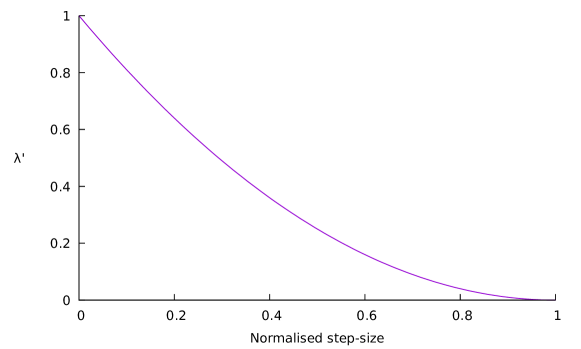
Figure 3: Normalised Canonical trade-off coefficient $\lambda^{\prime}=\frac{4{\eta}}{B^{[D-1]2}}\lambda$ vs normalised gradient-descent step-size $\frac{\|{\bf t}_{{\Delta}}^{[j]{\boxast}}\|_{\infty}}{B^{[D-1]}}$.

7 Application - Rademacher Complexity

Having established an exact representation of neural networks in finite neighbourhoods of weights and biases, established the link with RKBS theory and demonstrated that a gradient descent step is equivalent to a regularised step in RKBS by appropriate, a-posterior selection of scale factors and shadow weights (canonical scaling), we now consider an application of this framework to uniform convergence analysis using Rademacher complexity. The Rademacher complexity of a set $\mathcal{G}$ of real-valued functions is a measure of its capacity. Assuming training vectors ${\bf x}_{i}\sim\nu$ and Rademacher random variables $\epsilon_{i}\in\{-1,1\}$, the Rademacher complexity of $\mathcal{G}$ is (Mendelson, 2003):

$$\begin{array}[]{rl}\mathcal{R}_{N}\left(\mathcal{G}\right)&\!\!\!\!=\mathbb{E}_{\nu,\epsilon}\left[{\rm sup}_{f\in\mathcal{G}}\left|\frac{1}{N}{\sum}_{i}\epsilon_{i}f\left({\bf x}_{i}\right)\right|\right]\\ \end{array}$$

This may be used in uniform convergence analysis to bound how quickly the empirical risk converges to the expected risk, typically of the form:

$$\begin{array}[]{l}\left|\overline{R}\left(g\right)-R_{E}\left(g\right)\right|\leq c\mathcal{R}_{N}\left(\mathcal{G}\right)+\mbox{excess risk}\end{array}$$

The following theorem demonstrates how our framework may be used to bound Rademacher complexity for a scalar-output neural network:

Theorem 2.

Let $\epsilon,\chi\in(0,1)$ and for a given neural network with initial weights ${\bf W}_{\mathcal{O}}$, and let ${\bf W}_{\Delta}^{\boxast}$ be the weight-step for this derived from back-propagation satisfying the conditions set out in corollary 10. Then $f_{\Delta}^{\boxast}\in\mathcal{F}^{\bullet}$, where the Rademacher complexity of $\mathcal{F}^{\bullet}$ is bounded as:

$$\begin{array}[]{l}\frac{\mathcal{R}_{N}\left(\mathcal{F}^{\bullet}\right)}{H^{[D-1]}}\leq\sqrt{\frac{\bar{\sigma}^{[D-1]}\left(\left(1-\epsilon\right)\sqrt{\rho^{[D-1]}}\right)}{N}{\frac{\left\|{\bf t}_{{\Delta}}^{[D-1]{\boxast}}\right\|_{\infty}^{2}}{\frac{1}{1-\chi}B^{[D-1]2}-\left\|{\bf t}_{{\Delta}}^{[D-1]{\boxast}}\right\|_{\infty}^{2}}}}\end{array}$$

The proof of this theorem is a straightforward application of theorem 1 (see proof of theorem 11 in the appendix for details). Apart from the usual $\frac{1}{N}$ scaling this theorem is very different from typical bounds on Rademacher complexity, as it directly bounds the complexity using the size of the weight-step for a single iteration of gradient descent. Note:

• By the properties of Rademacher complexity (Bartlett and Mendelson, 2002, Theorem 12) the complexity of the trained neural network after $T$ iterations may be bounded by a simple summation of the bounds on each step. This supports the practice of using early-stopping to prevent overfitting in neural networks.

• The size of the back-propogation weight-step scales propotionally with the learning rate, so for sufficiently small learning rates we find:

  $$\begin{array}[]{l}\frac{\mathcal{R}_{N}\left(\mathcal{F}^{\bullet}\right)}{H^{[D-1]}}\lessapprox\sqrt{\frac{\bar{\sigma}^{[D-1]}\left(\left(1-\epsilon\right)\sqrt{\rho^{[D-1]}}\right)}{N}}\left\|{\bf t}_{{\Delta}}^{[D-1]{\boxast}}\right\|_{\infty}\end{array}$$

  However as the learning rate increases the bound will increase at an accelerating rate. This supports the lower learning rates act as a form of regularisation in neural network training.

To finish we consider a concrete example. Assume a $2$-layer network with a scalar output ($D=2$, $n=H^{[1]}=1$) with activation functions $\tau^{[0]}=\tau^{[1]}={\rm tanh}$ (so $\rho^{[0]}=\rho^{[1]}=\frac{\pi}{2}$ and $\tau^{(1)[0]}(\zeta),\tau^{(1)[1]}(\zeta)\in[-1,1]$. The form of $\sigma_{z,z^{\prime}}^{[j]}$ is non-trivial (see appendix F for details), but it is not difficult to see that $\overline{\sigma}^{[j]}=\sigma_{0,0}^{[j]}$, so, using the power-series about $0$:

$$\begin{array}[]{rl}\overline{\sigma}^{[0]}\left(\zeta\right)=\overline{\sigma}^{[1]}\left(\zeta\right)=\mathop{\sum}\limits_{m=1}^{\infty}\left(\frac{2^{2m}\left(2^{2m}-1\right)B_{2m}}{(2m)!}\right)^{2}\zeta^{2m-1}\\ \end{array}$$

and moreover $s^{[0]2}=\alpha^{[0]2}/2+{m}/2{H^{[0]}}$ and $s^{[1]2}=\alpha^{[1]2}/2+H^{[0]}$. Using our assumptions and the back-propagation equations, it is not difficult to see that:

$$\begin{array}[]{rl}\left\|{\bf t}_{{\Delta}}^{[0]{\boxast}}\right\|_{\infty}^{2}&\!\!\!\!\leq 2{\eta}^{2}N^{2}L_{E}^{2}\left\|{\bf W}_{{\mathcal{O}}}^{[1]}\right\|_{F}^{2}\left(1+\alpha^{[0]2}\right)\\ \left\|{\bf t}_{{\Delta}}^{[1]{\boxast}}\right\|_{\infty}^{2}&\!\!\!\!\leq 2{\eta}^{2}N^{2}L_{E}^{2}\left(1+\alpha^{[1]2}\right)\\ \end{array}$$

and $B^{[1]}=\frac{\left(1-\chi\right)^{2}\left(1-\epsilon\right)\sqrt{\frac{\pi}{2}}}{\frac{1}{2}\alpha^{[1]2}+H^{[0]}}$. Assuming a learning rate:

$$\begin{array}[]{rl}{\eta}=s{\frac{\left(1-\chi\right)}{NL_{E}\sqrt{2\left(1+\alpha^{[1]2}\right)}}\sqrt{\frac{\left(1-\epsilon\right)\sqrt{\frac{\pi}{2}}}{\frac{1}{2}\alpha^{[1]2}+H^{[0]}}}}\end{array}$$

where $0<s\ll 1$ - which follows the practice of scaling the learning rate inversely with the batch size and the network width - we obtain the following Rademacher complexity bound for the neural network trained for $T$ iterations:

$$\begin{array}[]{l}\frac{\mathcal{R}_{N}\left(\mathcal{F}^{\bullet}\right)}{H^{[D-1]}}\lessapprox sT\sqrt{2\frac{\bar{\sigma}^{[D-1]}\left(\left(1-\epsilon\right)\sqrt{\frac{\pi}{2}}\right)}{N}}\frac{\left(1-\chi\right)^{2}\left(1-\epsilon\right)\sqrt{\frac{\pi}{2}}}{\frac{1}{2}\alpha^{[1]2}+H^{[0]}}\end{array}$$

which we note scales inversely with the both the number of training vectors $N$ and the width of the network $H^{[0]}$.

8 Conclusions and Future Directions

In this paper we have established a connection between neural network training using gradient descent and regularised learning in reproducing kernel Banach space. We have introduced an exact representation of the behaviour of neural networks as the weights and biases are varied in a finite neighbourhood of some initial weights and biases in terms of an inner product of two feature maps, one from data space to feature space, the other from weight-step space to feature space. Using this, we showed that the change in neural network behaviour due to a single iteration of back-propagation lies in a reproducing kernel Banach space, and moreover that the weight-step found by back-propagation can be exactly replicated through regularised risk minimisation in RKBS. Subsequently we presented an upper bound on the Rademacher complexity of neural networks applicable to both the over- and under-parametrised regimes, and discussed how this bound depends on learning rate, dataset size, network width and the number of training iterations used.

With regard to future work we foresee a number of useful directions. First, the analysis should be extended to non-smooth activation functions such as ReLU, presumably by modifying the feature map using a representation other than a power series expansion. Second, the precise influence of the learning rate needs to be further explicated, along with other details of Theorem 1. With regard to the neural neighbourhood kernels themselves, it would be helpful if these could be reduced to closed form to allow them to be used in practice. Finally, more work is needed to understand the impact of the depth of the network on this theory.

Appendix A Derivations and Proofs.

Our goal in this supplement is to present all derivations and proofs relevant to our paper, and also any additional material and description that may be useful.

We assume a fully-connected, $D$-layer feedforward neural network ${\bf f}:({\mathbb{X}}\subseteq{\mathbb{R}}^{n})\to({\mathbb{Y}}\subseteq{\mathbb{R}}^{m})$ with layers of widths $H^{[0]},H^{[1]},\ldots,H^{[D-1]}$, where $H^{[D-1]}=m$ and we define $H^{[-1]}=n$. We assume layer $j\in{\mathbb{N}}_{D}$ (we use the convention $j\in{\mathbb{N}}_{D}$ throughout) is made up of neurons with the same activation function $\tau^{[j]}:{\mathbb{R}}\to{\mathbb{R}}$. The network is defined recursively:

$$\begin{array}[]{ll}\begin{array}[]{rl}{\bf f}\left({\bf x}\right)&\!\!\!\!={\bf x}^{[D]}\in{\mathbb{R}}^{H^{[D-1]}}\\ \end{array}&\\ \begin{array}[]{rl}{\bf x}^{[j+1]}&\!\!\!\!=\tau^{[j]}\left(\tilde{\bf x}^{[j]}\right)\in{\mathbb{R}}^{H^{[j]}}\\ \tilde{\bf x}^{[j]}&\!\!\!\!=\frac{1}{\sqrt{H^{[j]}}}{\bf W}^{[j]{\rm T}}{\bf x}^{[j]}+\alpha^{[j]}{\bf b}^{[j]}\in{\mathbb{R}}^{H^{[j]}}\\ \end{array}&\;\;\;\forall j\in{\mathbb{N}}_{D}\\ \begin{array}[]{rl}{\bf x}^{[0]}&\!\!\!\!={\bf x}\in{\mathbb{X}}\subset{\mathbb{R}}^{H^{[-1]}}\mbox{ ($H^{[-1]}=n$)}\\ \end{array}&\\ \end{array}$$ (16)

where ${\bf W}^{[j]}\in{\mathbb{R}}^{H^{[j-1]}\times H^{[j]}}$ and ${\bf b}^{[j]}\in{\mathbb{R}}^{H^{[j]}}$ are weights and biases, and $\alpha^{[j]}\in{\mathbb{R}}_{+}$ is a constant we will use later. We define the set of neural networks taking the form (16) as:

$$\begin{array}[]{rl}\mathcal{F}=\left\{\left.{\bf f}:{\mathbb{R}}^{n}\to{\mathbb{R}}^{m}\right|{\bf f}\mbox{ has form (\ref{eq:yall}) given }{\bf W}\in{\mathbb{W}}\right\}\end{array}$$ (17)

where ${\bf W}$ summarises the weights and biases in (16):

$$\begin{array}[]{rl}{\bf W}=\left(\left.\left({\bf W}^{[j]},{\bf b}^{[j]}\right)\right|j\in{\mathbb{N}}_{D}\right)\in{\mathbb{W}}=\mathop{\prod}\limits_{j\in{\mathbb{N}}_{D}}\left({\mathbb{R}}^{H^{[j-1]}\times H^{[j]}}\times{\mathbb{R}}^{H^{[j]}}\right)\\ \end{array}$$

Typically, the goal in neural network training is to take a training set and find weights and biases to minimise some measure of mismatch between the true training labels and the network’s predictions. For simplicity let us assume we wish to minimise:

$$\begin{array}[]{l}{\bf f}^{\star}=\mathop{\rm argmin}\limits_{{\bf f}\in\mathcal{F}}\sum_{k}E\left({\bf x}^{\{k\}},{\bf y}^{\{k\}},{\bf f}\left({\bf x}^{\{k\}}\right)\right)\end{array}$$ (18)

or, equivalently:

$$\begin{array}[]{l}{\bf W}^{\star}=\mathop{\rm argmin}\limits_{{\bf W}\in{\mathbb{W}}}\sum_{k}E\left({\bf x}^{\{k\}},{\bf y}^{\{k\}},{\bf f}_{\bf W}\left({\bf x}^{\{k\}}\right)\right)\end{array}$$ (19)

where ${\bf f}_{\bf W}$ is a network of the form (16) with weights and biases ${\bf W}$, ${\mathbb{D}}=\{({\bf x}^{\{k\}},{\bf y}^{\{k\}})\in{\mathbb{X}}\times{\mathbb{Y}}:k\in{\mathbb{N}}_{N}\}$ is a training set (we use the convention $k\in{\mathbb{N}}_{N}$ throughout), and $E:{\mathbb{X}}\times{\mathbb{Y}}\times{\mathbb{R}}^{m}\to{\mathbb{R}}$ is an error function defining the purpose of the network.

We make the following assumptions:

1. Input space: we assume ${\mathbb{X}}=[-{M}^{[-1]},{M}^{[-1]}]^{n}$.

2. Error function: we assume the error function $E:{\mathbb{X}}\times{\mathbb{Y}}\times{\mathbb{R}}^{m}\to{\mathbb{R}}$ is $\mathcal{C}^{1}$ and $L_{E}$-Lipschitz in its third argument.

3. Activation functions: we assume the activation functions $\tau^{[j]}:{\mathbb{R}}\to[-{M}^{[j]},{M}^{[j]}]^{H^{[j]}}$ are bounded and $\mathcal{C}^{\infty}$, and that $\tau^{[j]}$ has a power-series representations with region of convergence (ROC) at least $\rho^{[j]}\in{\mathbb{R}}_{+}$ around $z$ for all $z\in{\mathbb{R}}$, $j\in{\mathbb{N}}_{D}$.

4. Weight non-triviality: we assume ${\bf W}^{[j]}\neq{\bf 0}$ for all $j\in{\mathbb{N}}_{D}$ at all times during training.

5. Weight initialisation: we assume that initially $W_{i_{j},i_{j+1}}^{[j]},b_{i_{j+1}}^{[j]}\sim\mathcal{N}(0,1)$ (LeCun initialisation).

6. Training: we assume the network is trained using the back-propagation with learning rate ${\eta}\in{\mathbb{R}}_{+}$.

A.1 Review of Back-Propogation

We now give a brief review of back-propagation training, which is a systematic implementation of gradient descent on the weights and biases ${\bf W}$ to solve (19). Let us consider a single training iteration, where we start with initial weights and biases ${\bf W}_{\mathcal{O}}\in{\mathbb{W}}$ and calculate a weight-step ${\bf W}_{\Delta}^{\boxast}$ so that, after this iteration, ${\bf W}={\bf W}_{\mathcal{O}}+{\bf W}_{\Delta}^{\boxast}$, where:

$$\begin{array}[]{rl}{\bf W}_{\Delta}^{\boxast}&\!\!\!\!=-{\eta}\left.\frac{\partial}{\partial{\bf W}}\sum_{k}E\left({\bf x}^{\{k\}},{\bf y}^{\{k\}},{\bf f}_{\bf W}\left({\bf x}^{\{k\}}\right)\right)\right|_{{\bf W}={\bf W}_{\mathcal{O}}}\end{array}$$

Denote the network activation prior to the iteration given input ${\bf x}$ as:

$$\begin{array}[]{ll}\begin{array}[]{rl}{\bf f}_{\mathcal{O}}\left({\bf x}\right)&\!\!\!\!={\bf x}_{\mathcal{O}}^{[D]}\\ \end{array}&\\ \begin{array}[]{rl}{\bf x}_{\mathcal{O}}^{[j+1]}&\!\!\!\!=\tau^{[j]}\left(\tilde{\bf x}_{\mathcal{O}}^{[j]}\right)\\ \tilde{\bf x}_{\mathcal{O}}^{[j]}&\!\!\!\!=\frac{1}{\sqrt{H^{[j]}}}{\bf W}_{\mathcal{O}}^{[j]{\rm T}}{\bf x}_{\mathcal{O}}^{[j]}+\alpha^{[j]}{\bf b}_{\mathcal{O}}^{[j]}\\ \end{array}&\\ \begin{array}[]{rl}{\bf x}_{\mathcal{O}}^{[0]}&\!\!\!\!={\bf x}\in{\mathbb{X}}\\ \end{array}&\\ \end{array}$$ (20)

for all layers $j\in{\mathbb{N}}_{D}$. The back-propagation iteration for layer $D-1$ is a gradient descent step with learning rate ${\eta}$, namely:

$$\begin{array}[]{rl}W_{{\Delta}i_{D-1},i_{D}}^{[D-1]{\boxast}}&\!\!\!\!=\left.-{\eta}\frac{\partial}{\partial W_{i_{D-1},i_{D}}^{[D-1]}}\sum_{k}E\left({\bf x}^{\{k\}},{\bf y}^{\{k\}},{\bf f}_{\bf W}\left({\bf x}^{\{k\}}\right)\right)\right|{\bf W}={\bf W}_{\mathcal{O}}\\ &\!\!\!\!=\left.-{\eta}\sum_{k,i^{\prime}_{D}}\nabla_{i^{\prime}_{D}}E\left({\bf x}^{\{k\}},{\bf y}^{\{k\}},{\bf f}_{\bf W}\left({\bf x}^{\{k\}}\right)\right)\frac{\partial}{\partial W_{i_{D-1},i_{D}}^{[D-1]}}f_{i^{\prime}_{D}}\left({\bf x}^{\{k\}}\right)\right|{\bf W}={\bf W}_{\mathcal{O}}\\ &\!\!\!\!=\left.-{\eta}\sum_{k,i^{\prime}_{D}}\nabla_{i^{\prime}_{D}}E\left({\bf x}^{\{k\}},{\bf y}^{\{k\}},{\bf f}_{\bf W}\left({\bf x}^{\{k\}}\right)\right)\frac{\partial}{\partial W_{i_{D-1},i_{D}}^{[D-1]}}x_{i^{\prime}_{D}}^{\{k\}[D]}\right|{\bf W}={\bf W}_{\mathcal{O}}\\ &\!\!\!\!=\left.-{\eta}\sum_{k,i^{\prime}_{D}}\nabla_{i^{\prime}_{D}}E\left({\bf x}^{\{k\}},{\bf y}^{\{k\}},{\bf f}_{\bf W}\left({\bf x}^{\{k\}}\right)\right)\frac{\partial}{\partial W_{i_{D-1},i_{D}}^{[D-1]}}\tau^{[D-1]}\left({\tilde{x}}_{i^{\prime}_{D}}^{\{k\}[D-1]}\right)\right|{\bf W}={\bf W}_{\mathcal{O}}\\ &\!\!\!\!=\left.-{\eta}\sum_{k,i^{\prime}_{D}}\nabla_{i^{\prime}_{D}}E\left({\bf x}^{\{k\}},{\bf y}^{\{k\}},{\bf f}_{\bf W}\left({\bf x}^{\{k\}}\right)\right)\tau^{[D-1](1)}\left({\tilde{x}}_{i^{\prime}_{D}}^{\{k\}[D-1]}\right)\frac{\partial}{\partial W_{i_{D-1},i_{D}}^{[D-1]}}{\tilde{x}}_{i^{\prime}_{D}}^{\{k\}[D-1]}\right|{\bf W}={\bf W}_{\mathcal{O}}\\ &\!\!\!\!=-{\eta}\frac{1}{\sqrt{H^{[D-1]}}}\sum_{k}\gamma_{{\mathcal{O}}i_{D}}^{\{k\}[D-1]}x_{{\mathcal{O}}i_{D-1}}^{\{k\}[D-1]}\\ \end{array}$$

where $\tau^{(r)}(z)=\frac{\partial^{r}}{\partial^{r}z}\tau(z)$ and:

$$\begin{array}[]{rl}\gamma_{{\mathcal{O}}i_{D}}^{\{k\}[D-1]}&\!\!\!\!=\nabla_{i_{D}}E\left({\bf x}^{\{k\}},{\bf y}^{\{k\}},{\bf f}_{\bf W}\left({\bf x}^{\{k\}}\right)\right)\tau^{[D-1](1)}\left(\tilde{x}_{{\mathcal{O}}i_{D}}^{\{k\}[D-1]}\right)\\ \end{array}$$

Subsequently:

$$\begin{array}[]{rl}W_{{\Delta}i_{D-2},i_{D-1}}^{[D-2]{\boxast}}&\!\!\!\!=\left.-{\eta}\frac{\partial}{\partial W_{i_{D-2},i_{D-1}}^{[D-2]}}\sum_{k}E\left({\bf x}^{\{k\}},{\bf y}^{\{k\}},{\bf f}\left({\bf x}^{\{k\}}\right)\right)\right|{\bf W}={\bf W}_{\mathcal{O}}\\ &\!\!\!\!=\left.-{\eta}\sum_{k,i^{\prime}_{D}}\gamma_{{\mathcal{O}}i^{\prime}_{D}}^{\{k\}[D-1]}\frac{\partial}{\partial W_{i_{D-2},i_{D-1}}^{[D-2]}}\tilde{x}_{i^{\prime}_{D}}^{\{k\}[D-1]}\right|{\bf W}={\bf W}_{\mathcal{O}}\\ &\!\!\!\!=\left.-{\eta}\frac{1}{\sqrt{H^{[D-1]}}}\sum_{k,i^{\prime}_{D},i^{\prime}_{D-1}}\gamma_{{\mathcal{O}}i^{\prime}_{D}}^{\{k\}[D-1]}W_{{\mathcal{O}}i^{\prime}_{D-1},i^{\prime}_{D}}^{[D-1]}\frac{\partial}{\partial W_{i_{D-2},i_{D-1}}^{[D-2]}}x_{i^{\prime}_{D-1}}^{\{k\}[D-1]}\right|{\bf W}={\bf W}_{\mathcal{O}}\\ &\!\!\!\!=\left.-{\eta}\frac{1}{\sqrt{H^{[D-1]}}}\sum_{k,i^{\prime}_{D},i^{\prime}_{D-1}}\gamma_{{\mathcal{O}}i^{\prime}_{D}}^{\{k\}[D-1]}W_{{\mathcal{O}}i^{\prime}_{D-1},i^{\prime}_{D}}^{[D-1]}\frac{\partial}{\partial W_{i_{D-2},i_{D-1}}^{[D-2]}}\tau^{[D-2]}\left(\tilde{x}_{i^{\prime}_{D-1}}^{\{k\}[D-2]}\right)\right|{\bf W}={\bf W}_{\mathcal{O}}\\ &\!\!\!\!=\left.-{\eta}\frac{1}{\sqrt{H^{[D-1]}}}\sum_{k,i^{\prime}_{D},i^{\prime}_{D-1}}\gamma_{{\mathcal{O}}i^{\prime}_{D}}^{\{k\}[D-1]}W_{{\mathcal{O}}i^{\prime}_{D-1},i^{\prime}_{D}}^{[D-1]}\tau^{[D-2](1)}\left(\tilde{x}_{i^{\prime}_{D-1}}^{\{k\}[D-2]}\right)\frac{\partial}{\partial W_{i_{D-2},i_{D-1}}^{[D-2]}}\tilde{x}_{i^{\prime}_{D-1}}^{\{k\}[D-2]}\right|{\bf W}={\bf W}_{\mathcal{O}}\\ &\!\!\!\!=\left.-{\eta}\frac{1}{\sqrt{H^{[D-1]}}}\sum_{k,i^{\prime}_{D-1}}\gamma_{{\mathcal{O}}i^{\prime}_{D-1}}^{\{k\}[D-2]}\frac{\partial}{\partial W_{i_{D-2},i_{D-1}}^{[D-2]}}\tilde{x}_{i^{\prime}_{D-1}}^{\{k\}[D-2]}\right|{\bf W}={\bf W}_{\mathcal{O}}\\ &\!\!\!\!=-{\eta}\frac{1}{\sqrt{H^{[D-1]}H^{[D-2]}}}\sum_{k}\gamma_{{\mathcal{O}}i_{D-1}}^{\{k\}[D-2]}x_{{\mathcal{O}}i_{D-2}}^{\{k\}[D-2]}\\ \end{array}$$

where:

$$\begin{array}[]{rl}\gamma_{{\mathcal{O}}i_{D-1}}^{\{k\}[D-2]}&\!\!\!\!=\sum_{i_{D}}\gamma_{{\mathcal{O}}i_{D}}^{\{k\}[D-1]}W_{{\mathcal{O}}i_{D-1},i_{D}}^{\{k\}[D-1]}\tau^{[D-2](1)}\left(\tilde{x}_{{\mathcal{O}}i_{D-1}}^{\{k\}[D-2]}\right)\end{array}$$

and so on through all layers. Summarising, for all $j\in{\mathbb{N}}_{D}$ (and using the MATLAB notation ${\bf A}_{:i}$ for column $i$ of matrix ${\bf A}$):

$$\begin{array}[]{rl}{\bf W}_{{\Delta}:i_{j+1}}^{[j]{\boxast}}&\!\!\!\!=-{\eta}\frac{1}{\sqrt{H^{[D-1]}H^{[D-2]}\ldots H^{[j+1]}}}\sum_{k}\gamma_{{\mathcal{O}}i_{j+1}}^{\{k\}[j]}\frac{1}{\sqrt{H^{[j]}}}{\bf x}_{{\mathcal{O}}}^{\{k\}[j]}\\ b_{{\Delta}:i_{j+1}}^{[j]{\boxast}}&\!\!\!\!=-{\eta}\frac{1}{\sqrt{H^{[D-1]}H^{[D-2]}\ldots H^{[j+1]}}}\sum_{k}\gamma_{{\mathcal{O}}i_{j+1}}^{\{k\}[j]}\alpha^{[j]}\\ \end{array}$$ (21)

where, recursively:

$$\begin{array}[]{rl}\gamma_{{\mathcal{O}}i_{j}}^{\{k\}[j-1]}&\!\!\!\!=\sum_{i_{j+1}}\gamma_{{\mathcal{O}}i_{j+1}}^{\{k\}[j]}W_{{\mathcal{O}}i_{j},i^{\prime}_{j+1}}^{[j]}\tau^{[j-1](1)}\left(\tilde{x}_{{\mathcal{O}}i_{j}}^{\{k\}[j-1]}\right)\\ \gamma_{{\mathcal{O}}i_{D}}^{\{k\}[D-1]}&\!\!\!\!=\nabla_{i_{D}}E\left({\bf x}^{\{k\}},{\bf y}^{\{k\}},{\bf f}\left({\bf x}^{\{k\}}\right)\right)\tau^{[D-1](1)}\left(\tilde{x}_{{\mathcal{O}}i_{D}}^{\{k\}[D-1]}\right)\\ \end{array}$$ (22)

Appendix B Dual Form of a Neural Network Step

Our first goal is to rewrite the neural network after a training iteration as:

$$\begin{array}[]{rl}{\bf f}\left({\bf x}\right)&\!\!\!\!={\bf f}_{\mathcal{O}}\left({\bf x}\right)+{\bf f}_{{\Delta}}\left({\bf x}\right)\\ \end{array}$$

where ${\bf f}_{\mathcal{O}}:({\mathbb{X}}\subset{\mathbb{R}}^{n})\to({\mathbb{Y}}\subset{\mathbb{R}}^{m})$ is the neural network before the iteration and ${\bf f}_{\Delta}:({\mathbb{X}}\subset{\mathbb{R}}^{n})\to{\mathbb{R}}^{m}$ is the change in network behaviour due to the change ${\bf W}_{\Delta}\in{\mathbb{W}}_{\mathcal{O}}$ in weights and biases for this iteration, so that:

$$\begin{array}[]{rl}{\bf f}_{{\Delta}}\left({\bf x}\right)&\!\!\!\!=\left<{{\bm{\Phi}}}_{{\mathcal{O}}}\left({\bf x}\right),{{\bm{\Psi}}}_{{\mathcal{O}}}\left({\bf W}_{{\Delta}}\right)\right>_{\mathcal{X}_{\mathcal{O}}\times\mathcal{W}_{\mathcal{O}}}\\ \end{array}$$

where:

$$\begin{array}[]{rl}{{\bm{\Phi}}}_{{\mathcal{O}}}&\!\!\!\!:{\mathbb{X}}\to\mathcal{X}_{\mathcal{O}}={\rm span}\left({{{\bm{\Phi}}}}_{\mathcal{O}}\left({\mathbb{X}}\right)\right)\subset{\mathbb{R}}^{\infty\times m}\\ {{\bm{\Psi}}}_{{\mathcal{O}}}&\!\!\!\!:{\mathbb{W}}_{\mathcal{O}}\to\mathcal{W}_{\mathcal{O}}={\rm span}\left({{{\bm{\Psi}}}}_{\mathcal{O}}\left({\mathbb{W}}_{\mathcal{O}}\right)\right)\subset{\mathbb{R}}^{\infty\times m}\\ \end{array}$$

are feature maps;

$$\begin{array}[]{rl}{\mathbb{W}}_{\mathcal{O}}\subset\mathop{\prod}\limits_{j\in{\mathbb{N}}_{D}}\left({\mathbb{R}}^{H^{[j-1]}\times H^{[j]}}\times{\mathbb{R}}^{H^{[j]}}\right)\\ \end{array}$$

and $\left<\cdot,\cdot\right>_{\mathcal{X}_{\mathcal{O}}\times\mathcal{W}_{\mathcal{O}}}:\mathcal{X}_{\mathcal{O}}\times\mathcal{W}_{\mathcal{O}}\to{\mathbb{R}}^{m}$ is the bilinear form:

$$\begin{array}[]{rl}\left<{{\bm{\Xi}}},{{\bm{\Omega}}}\right>_{\mathcal{X}_{\mathcal{O}}\times\mathcal{W}_{\mathcal{O}}}&\!\!\!\!={\rm diag}\left({{\bm{\Xi}}}^{\rm T}{{\bm{\Omega}}}\right)\end{array}$$

Moreover we aim to show that the feature maps are entirely defined by:

1. The structure of the network - that is, the number of layers, their widths and activation functions.

2. The weights and biases ${\bf W}_{\mathcal{O}}\in{\mathbb{W}}$ before the iteration.

We will then use this to construct appropriate norms for the weight feature space $\mathcal{W}_{\mathcal{O}}$ and data feature space $\mathcal{X}_{\mathcal{O}}$, which will allow us to prove that ${\bf f}_{{\Delta}}$ lies in a reproducing kernel Banach space, and analyse the complexity and convergence of the neural network.

B.1 Preliminary: Power Series Notation

The approach taken here is direct - we construct a power series expansion of the network without truncation and rearrange the terms to separate the resulting summation into the desired form. To make the process easier we define:

$$\begin{array}[]{c}\begin{array}[]{rlrlrl}{{\bm{\varrho}}}\left({\bf a},{\bf d}\right)&\!\!\!\!=\left[\begin{array}[]{c}a_{0}{\bf d}^{\otimes 1}\\ a_{1}{\bf d}^{\otimes 2}\\ \vdots\\ \end{array}\right]\\ \end{array}\end{array}$$

noting that this is linear in the elementwise (Hadamard) product, so:

$$\begin{array}[]{rl}{{\bm{\varrho}}}\left({\bf a},{\bf d}\right)\odot{{\bm{\varrho}}}\left({\bf a}^{\prime},{\bf d}^{\prime}\right)&\!\!\!\!={{\bm{\varrho}}}\left({\bf a}\odot{\bf a}^{\prime},{\bf d}\odot{\bf d}^{\prime}\right)\\ \end{array}$$

Using this notation it is straightforward to obtain the following useful shorthand for the multi-dimensional Taylor expansion (using the smoothness assumption) of $\tau^{[j]}:{\mathbb{R}}\to{\mathbb{R}}$ about $z\in{\mathbb{R}}$ for ${\bf c},{\bf c}^{\prime}\in{\mathbb{R}}^{p}$, $\left|\left<{\bf c},{\bf c}^{\prime}\right>\right|\leq\rho^{[j]}$:

$$\begin{array}[]{rl}\tau^{[j]}\left(z+\left<{\bf c},{\bf c}^{\prime}\right>\right)&\!\!\!\!=\tau^{[j]}\left(z\right)+\left<{{\bm{\varrho}}}\left({\bf g}^{[j]}\left(z\right),{\bf c}\right),{{\bm{\varrho}}}\left({\bf 1}_{\infty},{\bf c}^{\prime}\right),\right>\\ \end{array}$$ (23)

where the derivatives of $\tau^{[j]}$ at $z$ are encoded as:

$$\begin{array}[]{rl}{\bf g}^{[j]}\left(z\right)&\!\!\!\!=\left[\begin{array}[]{c}\frac{1}{1!}\tau^{[j](1)}\left(z\right)\\ \frac{1}{2!}\tau^{[j](2)}\left(z\right)\\ \frac{1}{3!}\tau^{[j](3)}\left(z\right)\\ \vdots\\ \end{array}\right]\end{array}$$

and $\tau^{[j](r)}(z)=\frac{\partial^{r}}{\partial z^{r}}\tau^{[j]}(z)$.

B.2 Feature Maps for Neural Networks

We represent the operation before and after the iteration, as well as the change due to the iteration, as:

$$\begin{array}[]{c}\begin{array}[]{ccccc}\left(\!\!\!\begin{array}[]{c}\mbox{{\bf Before Iteration}}\\ \begin{array}[]{l}{\bf f}_{\mathcal{O}}\left({\bf x}\right)={\bf x}_{\mathcal{O}}^{[D]}\in{\mathbb{Y}}\\ {\bf x}_{\mathcal{O}}^{[j+1]}=\tau^{[j]}\left(\tilde{\bf x}_{\mathcal{O}}^{[j]}\right)\\ \tilde{\bf x}_{\mathcal{O}}^{[j]}=\frac{1}{\sqrt{H^{[j]}}}{\bf W}_{\mathcal{O}}^{[j]{\rm T}}{\bf x}_{\mathcal{O}}^{[j]}+\alpha^{[j]}{\bf b}_{\mathcal{O}}^{[j]}\\ {\bf x}_{\mathcal{O}}^{[0]}={\bf x}\in{\mathbb{X}}\\ \end{array}\\ \end{array}\!\!\!\right)\par&\!\!\!+\!\!\!&\left(\!\!\!\begin{array}[]{c}\mbox{{\bf Weight-step Change}}\\ \begin{array}[]{l}{\bf f}^{{\;}^{{{\;}^{\;}}}}_{{\Delta}_{{\;}_{{{\;}_{\;}}}}}\!\!\!\!\!\left({\bf x}\right)={\bf f}\left({\bf x}\right)-{\bf f}_{\mathcal{O}}\left({\bf x}\right)\\ {\bf x}_{{\Delta}_{{\;}_{{{\;}_{\;}}}}}^{[j+1]}={\bf x}^{[j+1]}-{\bf x}_{\mathcal{O}}^{[j+1]}\\ \tilde{\bf x}_{{\Delta}_{{\;}_{{{\;}_{\;}}}}}^{[j]}\!\!\!\!=\tilde{\bf x}^{[j]}-\tilde{\bf x}_{\mathcal{O}}^{[j]}\\ {\bf x}_{\Delta}^{[0]}={\bf x}\in{\bf 0}_{n}\\ \end{array}\\ \end{array}\!\!\!\right)\par&\!\!\!=\!\!\!&\left(\!\!\!\begin{array}[]{c}\mbox{{\bf After Iteration}}\\ \begin{array}[]{l}{\bf f}^{{\;}^{{{\;}^{\;}}}}_{{\;}_{{\;}_{{\;}_{\;}}}}\!\!\!\!\!\!\left({\bf x}\right)={\bf x}^{[D]}\in{\mathbb{Y}}\\ {\bf x}_{{\;}_{{\;}_{{\;}_{\;}}}}^{[j+1]}\!=\tau^{[j]}\left(\tilde{\bf x}_{{\;}_{{\;}_{\;}}}^{[j]}\!\right)\\ \tilde{\bf x}_{{\;}_{{\;}_{{\;}_{\;}}}}^{[j]}\!=\frac{1}{\sqrt{H^{[j]}}}{\bf W}^{[j]{\rm T}}{\bf x}^{[j]}+\alpha^{[j]}{\bf b}^{[j]}\\ {\bf x}_{{\;}_{{\;}_{{\;}_{\;}}}}^{[0]}\!={\bf x}\in{\mathbb{X}}\\ \end{array}\\ \end{array}\!\!\!\right)\par\end{array}\\ \Uparrow_{{\;}_{{\;}_{\;}}}^{{\;}^{{\;}^{{\;}^{\;}}}}\!\!\\ \left(\begin{array}[]{l}{\bf x}_{\Delta}^{[j+1]}=\tau^{[j]}\left(\tilde{\bf x}_{\mathcal{O}}^{[j]}+\tilde{\bf x}_{\Delta}^{[j]}\right)-\tau^{[j]}\left(\tilde{\bf x}_{\mathcal{O}}^{[j]}\right)\\ \tilde{\bf x}_{\Delta}^{[j]}=\frac{1}{\sqrt{H^{[j]}}}{\bf W}_{\Delta}^{[j]{\rm T}}\left({\bf x}_{\mathcal{O}}^{[j]}+{\bf x}_{\Delta}^{[j]}\right)+\frac{1}{\sqrt{H^{[j]}}}{\bf W}_{\mathcal{O}}^{[j]{\rm T}}{\bf x}_{\Delta}^{[j]}+\alpha^{[j]}{\bf b}_{\Delta}^{[j]}\\ \end{array}\right)\\ \end{array}$$ (24)

Our goal is to write ${\bf f}_{\Delta}:{\mathbb{X}}\to{\mathbb{R}}^{m}$ as:

$$\begin{array}[]{rl}{\bf f}_{{\Delta}}\left({\bf x}\right)&\!\!\!\!=\left<{{\bm{\Phi}}}_{{\mathcal{O}}}\left({\bf x}\right),{{\bm{\Psi}}}_{{\mathcal{O}}}\left({\bf W}_{{\Delta}}\right)\right>_{\mathcal{X}_{\mathcal{O}}\times\mathcal{W}_{\mathcal{O}}}\\ \end{array}$$

where ${{\bm{\Phi}}}_{{\mathcal{O}}}:{\mathbb{X}}\to\mathcal{X}_{\mathcal{O}}$ and ${{\bm{\Psi}}}_{{\mathcal{O}}}:{\mathbb{W}}_{\mathcal{O}}\to\mathcal{W}_{\mathcal{O}}$ are feature maps and $\left<{{\bm{\Xi}}},{{\bm{\Omega}}}\right>_{\mathcal{X}_{\mathcal{O}}\times\mathcal{W}_{\mathcal{O}}}={\rm diag}({{\bm{\Xi}}}^{\rm T}{{\bm{\Omega}}})$ is a bilinear form.

Starting with the first layer of the network, it is not difficult to see that:

$$\begin{array}[]{rl}\tilde{x}_{i_{1}}^{[0]}&\!\!\!\!=\tilde{x}_{{\mathcal{O}}i_{1}}^{[0]}+\tilde{x}_{{\Delta}i_{1}}^{[0]}\\ \tilde{x}_{{\mathcal{O}}i_{1}}^{[0]}&\!\!\!\!=\frac{1}{\sqrt{H^{[0]}}}{\bf W}_{{\mathcal{O}}:i_{1}}^{[0]{\rm T}}{\bf x}_{\mathcal{O}}+\alpha^{[0]}b_{{\mathcal{O}}i_{1}}^{[0]}\\ \tilde{x}_{{\Delta}i_{1}}^{[0]}&\!\!\!\!=\frac{1}{\sqrt{H^{[0]}}}{\bf W}_{{\Delta}:i_{1}}^{[0]{\rm T}}{\bf x}_{\mathcal{O}}+\alpha^{[0]}b_{{\Delta}i_{1}}^{[0]}\\ &\!\!\!\!=\left<{\mu}_{i_{1}}^{[0]}\left[\begin{array}[]{c}\frac{1}{\sqrt{2}}\alpha^{[0]}\\ \frac{1}{\sqrt{H^{[0]}}}\frac{1}{\sqrt{2}}{\bf x}_{\mathcal{O}}\\ \end{array}\right],\frac{1}{{\mu}_{i_{1}}^{[0]}}\left[\begin{array}[]{c}\sqrt{2}{b}_{{\Delta}i_{1}}^{[0]}\\ \sqrt{2}{\bf W}_{{\Delta}:i_{1}}^{[0]}\\ \end{array}\right]\right>\\ \end{array}$$

where ${\mu}^{[0]}_{i_{1}}\in{\mathbb{R}}_{+}$ are parameters we call scale factors, and ${\bf A}_{:l}$ for column $l$ of matrix ${\bf A}$. The scale factors will always cancel out in our representation of ${\bf f}$, but will be important later when we place norms on feature space. Using a power series expansion as per (23), if $\|\tilde{\bf x}_{\Delta}^{[0]}\|_{\infty}\leq\rho^{[0]}$:

$$\begin{array}[]{rl}{\bf x}^{[1]}&\!\!\!\!=\left[\tau^{[0]}\left(\tilde{x}_{i_{1}}^{[0]}\right)\right]_{i_{1}}=\left[\tau^{[0]}\left(\tilde{x}_{{\mathcal{O}}i_{1}}^{[0]}+\tilde{x}_{{\Delta}i_{1}}^{[0]}\right)\right]_{i_{1}}\\ &\!\!\!\!={\bf x}_{\mathcal{O}}^{[1]}+\left[\left<{{\bm{\varrho}}}\left({\bf g}^{[0]}\left(\tilde{x}_{{\mathcal{O}}i_{1}}^{[0]}\right),{\mu}_{i_{1}}^{[0]}\left[\begin{array}[]{c}\frac{1}{\sqrt{2}}\alpha^{[0]}\\ \frac{1}{\sqrt{H^{[0]}}}\frac{1}{\sqrt{2}}{\bf x}_{\mathcal{O}}\\ \end{array}\right]\right),{{\bm{\varrho}}}\left({\bf 1}_{\infty},\frac{1}{{\mu}_{i_{1}}^{[0]}}\left[\begin{array}[]{c}\sqrt{2}{b}_{{\Delta}i_{1}}^{[0]}\\ \sqrt{2}{\bf W}_{{\Delta}:i_{1}}^{[0]}\\ \end{array}\right]\right)\right>\right]_{i_{1}}\\ \end{array}$$

and hence:

$$\begin{array}[]{rl}{\bf x}_{\Delta}^{[1]}&\!\!\!\!=\left[\left<{{\bm{\Phi}}}_{{\mathcal{O}}:i_{1}}^{[0]}\left({\bf x}\right),{{\bm{\Psi}}}_{{\mathcal{O}}:i_{1}}^{[0]}\left({\bf W}_{\Delta}\right)\right>\right]_{i_{1}}\\ \end{array}$$

where:

$$\begin{array}[]{rl}{{\bm{\Phi}}}_{{\mathcal{O}}:i_{1}}^{[0]}\left({\bf x}\right)&\!\!\!\!={{\bm{\varrho}}}\left({\bf g}^{[0]}\left(\tilde{x}_{{\mathcal{O}}i_{1}}^{[0]}\right),{\mu}_{i_{1}}^{[0]}\left[\begin{array}[]{c}\frac{1}{\sqrt{2}}\alpha^{[0]}\\ \frac{1}{\sqrt{H^{[0]}}}\frac{1}{\sqrt{2}}{\bf x}_{\mathcal{O}}\\ \end{array}\right]\right)\\ {{\bm{\Psi}}}_{{\mathcal{O}}:i_{1}}^{[0]}\left({\bf W}_{\Delta}\right)&\!\!\!\!={{\bm{\varrho}}}\left({\bf 1}_{\infty},\frac{1}{{\mu}_{i_{1}}^{[0]}}\left[\begin{array}[]{c}\sqrt{2}{b}_{{\Delta}i_{1}}^{[0]}\\ \sqrt{2}{\bf W}_{{\Delta}:i_{1}}^{[0]}\\ \end{array}\right]\right)\\ \end{array}$$

Moving to the second layer, we see that:

$$\begin{array}[]{rl}\tilde{x}_{i_{2}}^{[1]}&\!\!\!\!=\tilde{x}_{{\mathcal{O}}i_{2}}^{[1]}+\tilde{x}_{{\Delta}i_{2}}^{[1]}\\ \tilde{x}_{{\mathcal{O}}i_{2}}^{[1]}&\!\!\!\!=\frac{1}{\sqrt{H^{[1]}}}{\bf W}_{{\mathcal{O}}:i_{2}}^{[1]{\rm T}}{\bf x}_{\mathcal{O}}^{[1]}+\alpha^{[1]}b_{{\mathcal{O}}i_{2}}^{[1]}\\ \tilde{x}_{{\Delta}i_{2}}^{[1]}&\!\!\!\!=\frac{1}{\sqrt{H^{[1]}}}{\bf W}_{{\Delta}:i_{2}}^{[1]{\rm T}}{\bf x}_{\mathcal{O}}^{[1]}+\frac{1}{\sqrt{H^{[1]}}}\left({\bf W}_{{\Delta}:i_{2}}^{[1]{\rm T}}+{\bf W}_{{\mathcal{O}}:i_{2}}^{[1]{\rm T}}\right){\bf x}_{\Delta}^{[1]}+\alpha^{[1]}b_{{\Delta}i_{2}}^{[1]}\\ &\!\!\!\!=\frac{1}{\sqrt{H^{[1]}}}{\bf W}_{{\Delta}:i_{2}}^{[1]{\rm T}}{\bf x}_{\mathcal{O}}^{[1]}+\frac{1}{\sqrt{H^{[1]}}}\sum_{i_{1}}\left(W_{{\mathcal{O}}{i_{1}},{i_{2}}}^{[1]}+W_{{\Delta}{i_{1}},{i_{2}}}^{[1]}\right)\left<{{\bm{\Phi}}}_{{\mathcal{O}}:i_{1}}^{[0]}\left({\bf x}\right),{{\bm{\Psi}}}_{{\mathcal{O}}:i_{1}}^{[0]}\left({\bf W}_{\Delta}\right)\right>+\alpha^{[1]}b_{{\Delta}i_{2}}^{[1]}\\ &\!\!\!\!=\left<{{\mu}}_{i_{2}}^{[1]}\left[\begin{array}[]{c}\left[\begin{array}[]{c}\frac{1}{\sqrt{2}}\alpha^{[1]}\\ \frac{1}{\sqrt{H^{[1]}}}{\bf x}_{\mathcal{O}}^{[1]}\\ \end{array}\right]\\ \left[\begin{array}[]{c}\frac{1}{{{\widetilde{\omega}}}_{i_{1},i_{2}}^{[1]}}\frac{{{\omega}}_{i_{1}}^{[1]}W_{{\mathcal{O}}i_{1},i_{2}}^{[1]}}{\sqrt{H^{[1]}}}{{\bm{\Phi}}}_{{\mathcal{O}}:i_{1}}^{[0]}\left({\bf x}\right)\\ \end{array}\right]_{i_{1}}\\ \left[\begin{array}[]{c}\frac{{{\omega}}_{i_{1}}^{[1]}}{\sqrt{H^{[1]}}}{{\bm{\Phi}}}_{{\mathcal{O}}:i_{1}}^{[0]}\left({\bf x}\right)\\ \end{array}\right]_{i_{1}}\\ \end{array}\right],\frac{1}{{{\mu}}_{i_{2}}^{[1]}}\left[\begin{array}[]{c}\left[\begin{array}[]{c}\sqrt{2}b_{{\Delta}i_{2}}^{[1]}\\ {\bf W}_{{\Delta}:i_{2}}^{[1]}\\ \end{array}\right]\\ \left[\begin{array}[]{c}{{\widetilde{\omega}}}_{i_{1},i_{2}}^{[1]}\frac{1}{{{\omega}}_{i_{1}}^{[1]}}{{\bm{\Psi}}}_{{\mathcal{O}}:i_{1}}^{[0]}\left({\bf W}_{\Delta}\right)\\ \end{array}\right]_{i_{1}}\\ \left[\begin{array}[]{c}\frac{W_{{\Delta}i_{1},i_{2}}^{[1]}}{{{\omega}}_{i_{1}}^{[1]}}{{\bm{\Psi}}}_{{\mathcal{O}}:i_{1}}^{[0]}\left({\bf W}_{\Delta}\right)\\ \end{array}\right]_{i_{1}}\\ \end{array}\right]\right>\\ \end{array}$$

where ${\mu}_{i_{2}}^{[1]}\in{\mathbb{R}}_{+}$ are scale factors and ${{\omega}}_{i_{1}}^{[1]},{{\widetilde{\omega}}}_{i_{1},i_{2}}^{[1]}\in{\mathbb{R}}^{+}$ are shadow weights (note that both the shadow weights and scale factors cancel in the inner product). Taking the Taylor expansion and using the properties of ${{\bm{\varrho}}}$ we see that, provided $\|\tilde{\bf x}_{{\Delta}}^{[1]}\|_{\infty}\leq\rho^{[1]}$:

$${{\begin{array}[]{rl}{\bf x}_{\Delta}^{[2]}&\!\!\!\!=\left[\left<{{\bm{\Phi}}}_{{\mathcal{O}}:i_{2}}^{[1]}\left({\bf x}\right),{{\bm{\Psi}}}_{{\mathcal{O}}:i_{2}}^{[1]}\left({\bf W}_{\Delta}\right)\right>\right]_{i_{2}}\\ \end{array}}}$$

where:

$${{\begin{array}[]{rl}{{\bm{\Phi}}}_{{\mathcal{O}}:i_{2}}^{[1]}\left({\bf x}\right)&\!\!\!\!={{\bm{\varrho}}}\left({\bf g}^{[1]}\left(\tilde{x}_{{\mathcal{O}}i_{2}}^{[1]}\right),{{\mu}}_{i_{2}}^{[1]}\left[\begin{array}[]{c}\left[\begin{array}[]{c}\frac{1}{\sqrt{2}}\alpha^{[1]}\\ \frac{1}{\sqrt{H^{[1]}}}{\bf x}_{\mathcal{O}}^{[1]}\\ \end{array}\right]\\ \left[\begin{array}[]{c}\frac{1}{{{\widetilde{\omega}}}_{i_{1},i_{2}}^{[1]}}\frac{{{\omega}}_{i_{1}}^{[1]}W_{{\mathcal{O}}i_{1},i_{2}}^{[1]}}{\sqrt{H^{[1]}}}{{\bm{\Phi}}}_{{\mathcal{O}}:i_{1}}^{[0]}\left({\bf x}\right)\\ \end{array}\right]_{i_{1}}\\ \left[\begin{array}[]{c}\frac{{{\omega}}_{i_{1}}^{[1]}}{\sqrt{H^{[1]}}}{{\bm{\Phi}}}_{{\mathcal{O}}:i_{1}}^{[0]}\left({\bf x}\right)\\ \end{array}\right]_{i_{1}}\\ \end{array}\right]\right)\\ {{\bm{\Psi}}}_{{\mathcal{O}}:i_{2}}^{[1]}\left({\bf W}_{\Delta}\right)&\!\!\!\!={{\bm{\varrho}}}\left({\bf 1}_{\infty},\frac{1}{{{\mu}}_{i_{2}}^{[1]}}\left[\begin{array}[]{c}\left[\begin{array}[]{c}\sqrt{2}b_{{\Delta}i_{2}}^{[1]}\\ {\bf W}_{{\Delta}:i_{2}}^{[1]}\\ \end{array}\right]\\ \left[\begin{array}[]{c}{{\widetilde{\omega}}}_{i_{1},i_{2}}^{[1]}\frac{1}{{{\omega}}_{i_{1}}^{[1]}}{{\bm{\Psi}}}_{{\mathcal{O}}:i_{1}}^{[0]}\left({\bf W}_{\Delta}\right)\\ \end{array}\right]_{i_{1}}\\ \left[\begin{array}[]{c}\frac{W_{{\Delta}i_{1},i_{2}}^{[1]}}{{{\omega}}_{i_{1}}^{[1]}}{{\bm{\Psi}}}_{{\mathcal{O}}:i_{1}}^{[0]}\left({\bf W}_{\Delta}\right)\\ \end{array}\right]_{i_{1}}\\ \end{array}\right]\right)\\ \end{array}}}$$

Continuing, it is not difficult to see that, for any $j\in{\mathbb{N}}_{D}$, if:

$${{\begin{array}[]{rl}{\bf x}_{\Delta}^{[j]}&\!\!\!\!=\left[\left<{{\bm{\Phi}}}_{{\mathcal{O}}:i_{j}}^{[j-1]}\left({\bf x}\right),{{\bm{\Psi}}}_{{\mathcal{O}}:i_{j}}^{[j-1]}\left({\bf W}_{\Delta}\right)\right>\right]_{i_{j}}\\ \end{array}}}$$

then, with scale factors ${\mu}_{i_{j+1}}^{[j]}\in{\mathbb{R}}_{+}$ and shadow weights ${\omega}_{i_{j}}^{[j]},{\widetilde{\omega}}_{i_{j},i_{j+1}}^{[j]}\in{\mathbb{R}}_{+}$:

$$\begin{array}[]{rl}\tilde{x}_{i_{j+1}}^{[j]}&\!\!\!\!=\tilde{x}_{{\mathcal{O}}i_{j+1}}^{[j]}+\tilde{x}_{{\Delta}i_{j+1}}^{[j]}\\ \tilde{x}_{{\mathcal{O}}i_{j+1}}^{[j]}&\!\!\!\!=\frac{1}{\sqrt{H^{[j]}}}{\bf W}_{{\mathcal{O}}:i_{j+1}}^{[j]{\rm T}}{\bf x}_{\mathcal{O}}^{[j]}+\alpha^{[j]}b_{{\mathcal{O}}i_{j+1}}^{[j]}\\ \tilde{x}_{{\Delta}i_{j+1}}^{[j]}&\!\!\!\!=\frac{1}{\sqrt{H^{[j]}}}{\bf W}_{{\Delta}:i_{j+1}}^{[j]{\rm T}}{\bf x}_{\mathcal{O}}^{[j]}+\frac{1}{\sqrt{H^{[j]}}}\left({\bf W}_{{\Delta}:i_{j+1}}^{[j]{\rm T}}+{\bf W}_{{\mathcal{O}}:i_{j+1}}^{[j]{\rm T}}\right){\bf x}_{\Delta}^{[j]}+\alpha^{[j]}b_{{\Delta}i_{j+1}}^{[j]}\\ &\!\!\!\!=\frac{1}{\sqrt{H^{[j]}}}{\bf W}_{{\Delta}:i_{j+1}}^{[j]{\rm T}}{\bf x}_{\mathcal{O}}^{[j]}+\frac{1}{\sqrt{H^{[j]}}}\sum_{i_{j}}\left(W_{{\mathcal{O}}{i_{j}}{i_{j+1}}}^{[j]}+W_{{\Delta}{i_{j}}{i_{j+1}}}^{[j]}\right)\left<{{\bm{\Phi}}}_{{\mathcal{O}}:i_{j}}^{[j-1]}\left({\bf x}\right),{{\bm{\Psi}}}_{{\mathcal{O}}:i_{j}}^{[j-1]}\left({\bf W}_{\Delta}\right)\right>+\alpha^{[j]}b_{{\Delta}i_{j+1}}^{[j]}\\ &\!\!\!\!=\left<{{\mu}}_{i_{j+1}}^{[j]}\left[\begin{array}[]{c}\left[\begin{array}[]{c}\frac{1}{\sqrt{2}}\alpha^{[j]}\\ \frac{1}{\sqrt{H^{[j]}}}{\bf x}_{\mathcal{O}}^{[j]}\\ \end{array}\right]\\ \left[\begin{array}[]{c}\frac{1}{{{\widetilde{\omega}}}_{i_{j},i_{j+1}}^{[j]}}\frac{{{\omega}}_{i_{j}}^{[j]}W_{{\mathcal{O}}i_{j},i_{j+1}}^{[j]}}{\sqrt{H^{[j]}}}{{\bm{\Phi}}}_{{\mathcal{O}}:i_{j}}^{[j-1]}\left({\bf x}\right)\\ \end{array}\right]_{i_{j}}\\ \left[\begin{array}[]{c}\frac{{{\omega}}_{i_{j}}^{[j]}}{\sqrt{H^{[j]}}}{{\bm{\Phi}}}_{{\mathcal{O}}:i_{j}}^{[j-1]}\left({\bf x}\right)\\ \end{array}\right]_{i_{j}}\\ \end{array}\right],\frac{1}{{{\mu}}_{i_{j+1}}^{[j]}}\left[\begin{array}[]{c}\left[\begin{array}[]{c}\sqrt{2}b_{{\Delta}i_{j+1}}^{[j]}\\ {\bf W}_{{\Delta}:i_{j+1}}^{[j]}\\ \end{array}\right]\\ \left[\begin{array}[]{c}{{\widetilde{\omega}}}_{i_{j},i_{j+1}}^{[j]}\frac{1}{{{\omega}}_{i_{j}}^{[j]}}{{\bm{\Psi}}}_{{\mathcal{O}}:i_{j}}^{[j-1]}\left({\bf W}_{\Delta}\right)\\ \end{array}\right]_{i_{j}}\\ \left[\begin{array}[]{c}\frac{W_{{\Delta}i_{j},i_{j+1}}^{[j]}}{{{\omega}}_{i_{j}}^{[j]}}{{\bm{\Psi}}}_{{\mathcal{O}}:i_{j}}^{[j-1]}\left({\bf W}_{\Delta}\right)\\ \end{array}\right]_{i_{j}}\\ \end{array}\right]\right>\\ \end{array}$$

so, provided $\|\tilde{\bf x}_{{\Delta}}^{[j]}\|_{\infty}\leq\rho^{[j]}$, we have:

$${{\begin{array}[]{rl}{\bf x}_{\Delta}^{[j+1]}&\!\!\!\!=\left[\left<{{\bm{\Phi}}}_{{\mathcal{O}}:i_{j+1}}^{[j]}\left({\bf x}\right),{{\bm{\Psi}}}_{{\mathcal{O}}:i_{j+1}}^{[j]}\left({\bf W}_{\Delta}\right)\right>\right]_{i_{j+1}}\\ \end{array}}}$$

where:

$$\begin{array}[]{rl}{{\bm{\Phi}}}_{{\mathcal{O}}:i_{j+1}}^{[j]}\left({\bf x}\right)&\!\!\!\!={{\bm{\varrho}}}\left({\bf g}^{[j]}\left(\tilde{x}_{{\mathcal{O}}i_{j+1}}^{[j]}\right),{{\mu}}_{i_{j+1}}^{[j]}\left[\begin{array}[]{c}\left[\begin{array}[]{c}\frac{1}{\sqrt{2}}\alpha^{[j]}\\ \frac{1}{\sqrt{H^{[j]}}}{\bf x}_{\mathcal{O}}^{[j]}\\ \end{array}\right]\\ \left[\begin{array}[]{c}\frac{1}{{{\widetilde{\omega}}}_{i_{j},i_{j+1}}^{[j]}}\frac{{{\omega}}_{i_{j}}^{[j]}W_{{\mathcal{O}}i_{j},i_{j+1}}^{[j]}}{\sqrt{H^{[j]}}}{{\bm{\Phi}}}_{{\mathcal{O}}:i_{j}}^{[j-1]}\left({\bf x}\right)\\ \end{array}\right]_{i_{j}}\\ \left[\begin{array}[]{c}\frac{{{\omega}}_{i_{j}}^{[j]}}{\sqrt{H^{[j]}}}{{\bm{\Phi}}}_{{\mathcal{O}}:i_{j}}^{[j-1]}\left({\bf x}\right)\\ \end{array}\right]_{i_{j}}\\ \end{array}\right]\right)\\ {{\bm{\Psi}}}_{{\mathcal{O}}:i_{j+1}}^{[j]}\left({\bf W}_{\Delta}\right)&\!\!\!\!={{\bm{\varrho}}}\left({\bf 1}_{\infty},\frac{1}{{{\mu}}_{i_{j+1}}^{[j]}}\left[\begin{array}[]{c}\left[\begin{array}[]{c}\sqrt{2}b_{{\Delta}i_{j+1}}^{[j]}\\ {\bf W}_{{\Delta}:i_{j+1}}^{[j]}\\ \end{array}\right]\\ \left[\begin{array}[]{c}{{\widetilde{\omega}}}_{i_{j},i_{j+1}}^{[j]}\frac{1}{{{\omega}}_{i_{j}}^{[j]}}{{\bm{\Psi}}}_{{\mathcal{O}}:i_{j}}^{[j-1]}\left({\bf W}_{\Delta}\right)\\ \end{array}\right]_{i_{j}}\\ \left[\begin{array}[]{c}\frac{W_{{\Delta}i_{j},i_{j+1}}^{[j]}}{{{\omega}}_{i_{j}}^{[j]}}{{\bm{\Psi}}}_{{\mathcal{O}}:i_{j}}^{[j-1]}\left({\bf W}_{\Delta}\right)\\ \end{array}\right]_{i_{j}}\\ \end{array}\right]\right)\\ \end{array}$$

Thus, by induction, so long as $\|\tilde{\bf x}_{{\Delta}}^{[j]}\|_{\infty}\leq\rho^{[j]}$ $\forall j$:

$$\begin{array}[]{rl}{\bf f}\left({\bf x}\right)&\!\!\!\!={\bf f}_{\mathcal{O}}\left({\bf x}\right)+{\bf f}_{{\Delta}}\left({\bf x}\right)\\ {\bf f}_{{\Delta}}\left({\bf x}\right)&\!\!\!\!=\left<{{\bm{\Phi}}}_{{\mathcal{O}}}\left({\bf x}\right),{{\bm{\Psi}}}_{{\mathcal{O}}}\left({\bf W}_{\Delta}\right)\right>_{\mathcal{X}_{\mathcal{O}}\times\mathcal{W}_{\mathcal{O}}}\end{array}$$ (25)

where:

$${{\begin{array}[]{rl}{{\bm{\Phi}}}_{{\mathcal{O}}}\left({\bf x}\right)&\!\!\!\!={{\bm{\Phi}}}_{{\mathcal{O}}}^{[D-1]}\left({\bf x}\right)\\ {{\bm{\Psi}}}_{{\mathcal{O}}}\left({\bf W}_{\Delta}\right)&\!\!\!\!={{\bm{\Psi}}}_{{\mathcal{O}}}^{[D-1]}\left({\bf W}_{\Delta}\right)\\ \end{array}}}$$

and, working recursively:

$${{\begin{array}[]{rl}\begin{array}[]{rl}{{\bm{\Phi}}}_{{\mathcal{O}}:i_{j+1}}^{[j]}\left({\bf x}\right)&\!\!\!\!=\left\{\begin{array}[]{ll}{{\bm{\varrho}}}\left({\bf g}^{[j]}\left(\tilde{x}_{{\mathcal{O}}i_{j+1}}^{[j]}\right),{{\mu}}_{i_{j+1}}^{[j]}\left[\begin{array}[]{c}\left[\begin{array}[]{c}\frac{1}{\sqrt{2}}\alpha^{[j]}\\ \frac{1}{\sqrt{H^{[j]}}}{\bf x}_{\mathcal{O}}^{[j]}\\ \end{array}\right]\\ \left[\begin{array}[]{c}\frac{1}{{{\widetilde{\omega}}}_{i_{j}i_{j+1}}^{[j]}}\frac{{{\omega}}_{i_{j}}^{[j]}W_{{\mathcal{O}}i_{j},i_{j+1}}^{[j]}}{\sqrt{H^{[j]}}}{{\bm{\Phi}}}_{{\mathcal{O}}:i_{j}}^{[j-1]}\left({\bf x}\right)\\ \end{array}\right]_{i_{j}}\\ \left[\begin{array}[]{c}\frac{{{\omega}}_{i_{j}}^{[j]}}{\sqrt{H^{[j]}}}{{\bm{\Phi}}}_{{\mathcal{O}}:i_{j}}^{[j-1]}\left({\bf x}\right)\\ \end{array}\right]_{i_{j}}\\ \end{array}\right]\right)&\mbox{if }j>0\\ {{\bm{\varrho}}}\left({\bf g}^{[0]}\left(\tilde{x}_{{\mathcal{O}}i_{1}}^{[0]}\right),{\mu}_{i_{1}}^{[0]}\left[\begin{array}[]{c}\frac{1}{\sqrt{2}}\alpha^{[0]}\\ \frac{1}{\sqrt{H^{[0]}}}\frac{1}{\sqrt{2}}{\bf x}_{\mathcal{O}}\\ \end{array}\right]\right)&\mbox{if }j=0\\ \end{array}\right.\\ {{\bm{\Psi}}}_{{\mathcal{O}}:i_{j+1}}^{[j]}\left({\bf W}_{{\Delta}}\right)&\!\!\!\!=\left\{\begin{array}[]{ll}{{\bm{\varrho}}}\left({\bf 1}_{\infty},\frac{1}{{{\mu}}_{i_{j+1}}^{[j]}}\left[\begin{array}[]{c}\left[\begin{array}[]{c}\sqrt{2}b_{{\Delta}i_{j+1}}^{[j]}\\ {\bf W}_{{\Delta}:i_{j+1}}^{[j]}\\ \end{array}\right]\\ \left[\begin{array}[]{c}{{\widetilde{\omega}}}_{i_{j},i_{j+1}}^{[j]}\frac{1}{{{\omega}}_{i_{j}}^{[j]}}{{\bm{\Psi}}}_{{\mathcal{O}}:i_{j}}^{[j-1]}\left({\bf W}_{\Delta}\right)\\ \end{array}\right]_{i_{j}}\\ \left[\begin{array}[]{c}\frac{W_{{\Delta}i_{j},i_{j+1}}^{[j]}}{{{\omega}}_{i_{j}}^{[j]}}{{\bm{\Psi}}}_{{\mathcal{O}}:i_{j}}^{[j-1]}\left({\bf W}_{\Delta}\right)\\ \end{array}\right]_{i_{j}}\\ \end{array}\right]\right)&\mbox{if }j>0\\ {{\bm{\varrho}}}\left({\bf 1}_{\infty},\frac{1}{{\mu}_{i_{1}}^{[0]}}\left[\begin{array}[]{c}\sqrt{2}{b}_{{\Delta}i_{1}}^{[0]}\\ \sqrt{2}{\bf W}_{{\Delta}:i_{1}}^{[0]}\\ \end{array}\right]\right)&\mbox{if }j=0\\ \end{array}\right.\\ \end{array}&\;\;\;\forall j\in{\mathbb{N}}_{D}\end{array}}}$$ (26)

with scale factors ${\mu}_{i_{j+1}}^{[j]}\in{\mathbb{R}}_{+}$ and shadow weights ${\omega}_{i_{j}}^{[j]},{\widetilde{\omega}}_{i_{j},i_{j+1}}^{[j]}\in{\mathbb{R}}_{+}$, $\forall j\in{\mathbb{N}}_{D}$.

To summarise, we have decomposed the neural network into the desired form (25) with the following components:

• A term ${\bf f}_{\mathcal{O}}\left({\bf x}\right)$ which is the network prior to the iteration evaluated on ${\bf x}$.

• A feature map ${{{\bm{\Phi}}}}_{{\mathcal{O}}}:{\mathbb{X}}\to\mathcal{X}_{\mathcal{O}}={\rm span}({{{\bm{\Phi}}}}_{\mathcal{O}}({\mathbb{X}}))\subset{\mathbb{R}}^{\infty\times m}$ from data input space to data feature space that is dependent only on the structure of the network (number of layers, their widths and the neuron types) and the weights and biases ${\bf W}_{\mathcal{O}}$ prior to the iteration.

• A feature map ${{\bm{\Psi}}}_{{\mathcal{O}}}:{\mathbb{W}}_{\mathcal{O}}\to\mathcal{W}_{\mathcal{O}}={\rm span}({{\bm{\Psi}}}_{\mathcal{O}}({\mathbb{W}}_{\mathcal{O}}))\subset{\mathbb{R}}^{\infty\times m}$ from weight-step input space to weight-step feature space that is dependent only on the structure of the network (number of layers and their widths).

B.3 Density of Feature Maps

In this section we prove a key property of the feature maps that will be required to prove that ${\bf f}_{{\Delta}}$ lies in the reproducing kernel Banach space. As a preliminary we show a consequence of the non-triviality assumption, namely:

Lemma 3.

Let ${\bf f}_{\mathcal{O}}\in\mathcal{F}$ be a neural network satisfying the non-triviality assumption. Then ${\bf f}_{\Delta}({\bf x})$ varies non-trivially with ${\bf x}$ (that is, it is non-constant).

Proof.

Recall that:

$$\begin{array}[]{rl}\tilde{\bf x}_{\Delta}^{[j]}&\!\!\!\!=\frac{1}{\sqrt{H^{[j]}}}{\bf W}_{\Delta}^{[j]{\rm T}}{\bf x}_{\mathcal{O}}^{[j]}+\frac{1}{\sqrt{H^{[j]}}}\left({\bf W}_{\mathcal{O}}^{[j]}+{\bf W}_{\Delta}^{[j]}\right)^{\rm T}{\bf x}_{\Delta}^{[j]}+\alpha^{[j]}{\bf b}_{\Delta}^{[j]}\\ &\!\!\!\!=\frac{1}{\sqrt{H^{[j]}}}{\bf W}_{\Delta}^{[j]{\rm T}}\left({\bf x}_{\mathcal{O}}^{[j]}+{\bf x}_{\Delta}^{[j]}\right)+\frac{1}{\sqrt{H^{[j]}}}{\bf W}_{\mathcal{O}}^{[j]{\rm T}}{\bf x}_{\Delta}^{[j]}+\alpha^{[j]}{\bf b}_{\Delta}^{[j]}\\ \end{array}$$

we want to know the conditions under which $\tilde{\bf x}_{\Delta}^{[D-1]}$ (and hence ${\bf f}_{{\Delta}}({\bf x})$) is a constant, independent of ${\bf x}$. Considering instead $\tilde{\bf x}_{\Delta}^{[j]}$, the only component in the above expression that depends on ${\bf x}$ is ${\bf x}_{\Delta}^{[j]}$, so $\tilde{\bf x}_{\Delta}^{[j]}$ is constant if either ${\bf W}_{\Delta}^{[j]}=-{\bf W}_{\mathcal{O}}^{[j]}$ or ${\bf x}_{\Delta}^{[j]}$ is constant independent of ${\bf x}$. So, recursing, we find that $\tilde{\bf x}_{\Delta}^{[D-1]}$ is constant (independent of ${\bf x}$) iff ${\bf W}_{\Delta}^{[j]}=-{\bf W}_{\mathcal{O}}^{[j]}$ for some $j\in{\mathbb{N}}_{D}$. However, recall that our non-triviality assumption explicitly rules out this case (which corresponds to trivial neural network post iteration), so ${\bf W}_{\Delta}^{[j]}\neq-{\bf W}_{\mathcal{O}}^{[j]}$ for all $j\in{\mathbb{N}}_{D}$, which suffices to demonstrate the desired result. ∎

Having addressed this preliminary, we now move to the main result for this section:

Lemma 4 (Density of Feature Maps).

The linear span of ${{{\bm{\Phi}}}}_{\mathcal{O}}({\mathbb{X}})$ is dense in $\mathcal{X}_{\mathcal{O}}$ with respect to $\left<\cdot,\cdot\right>_{\mathcal{X}_{\mathcal{O}}\times\mathcal{W}_{\mathcal{O}}}$; and the linear span of ${{\bm{\Psi}}}_{\mathcal{O}}({\mathbb{W}}_{\mathcal{O}})$ is dense in $\mathcal{W}_{\mathcal{O}}$ with respect to $\left<\cdot,\cdot\right>_{\mathcal{W}_{\mathcal{O}}\times\mathcal{X}_{\mathcal{O}}}$, where $\left<{{\bm{\Omega}}},{{\bm{\Xi}}}\right>_{\mathcal{W}_{\mathcal{O}}\times\mathcal{X}_{\mathcal{O}}}=\left<{{\bm{\Xi}}},{{\bm{\Omega}}}\right>_{\mathcal{X}_{\mathcal{O}}\times\mathcal{W}_{\mathcal{O}}}^{\rm T}$.

Proof.

By definition [Lin et al., 2022], the linear span ${\rm span}({{{\bm{\Phi}}}}_{\mathcal{O}}({\mathbb{X}}))$ of ${{{\bm{\Phi}}}}_{\mathcal{O}}({\mathbb{X}})$ is dense in $\mathcal{X}_{\mathcal{O}}$ with respect to $\left<\cdot,\cdot\right>_{\mathcal{X}_{\mathcal{O}}\times\mathcal{W}_{\mathcal{O}}}$ if for any ${{\bm{\Omega}}}_{\Delta}\in\mathcal{W}_{\mathcal{O}}$, the statement:

$$\begin{array}[]{l}\left<{{\bm{\Phi}}}_{\mathcal{O}}\left({\bf x}\right),{{\bm{\Omega}}}_{\Delta}\right>_{\mathcal{X}_{\mathcal{O}}\times\mathcal{W}_{\mathcal{O}}}={\bf 0}\;\;\;\forall{\bf x}\in{\mathbb{X}}\end{array}$$

implies that ${{\bm{\Omega}}}_{\Delta}={\bf 0}$. By definition $\mathcal{W}_{\mathcal{O}}={\rm span}({{{\bm{\Psi}}}}_{\mathcal{O}}({\mathbb{W}}_{\mathcal{O}}))$ so that ${{\bm{\Omega}}}_{\Delta}=\sum_{l}\tilde{\alpha}^{\{l\}}{\bf W}_{\Delta}^{\{l\}}$ for some $\tilde{\alpha}^{\{0\}},\tilde{\alpha}^{\{1\}},\ldots\in{\mathbb{R}}$, ${\bf W}_{{\Delta}}^{\{0\}},{\bf W}_{{\Delta}}^{\{1\}},\ldots\in{\mathbb{W}}_{\mathcal{O}}$, and hence:

$$\begin{array}[]{l}\left<{{\bm{\Phi}}}_{\mathcal{O}}\left({\bf x}\right),{{\bm{\Omega}}}_{\Delta}\right>_{\mathcal{X}_{\mathcal{O}}\times\mathcal{W}_{\mathcal{O}}}=\sum_{l}\tilde{\alpha}^{\{l\}}\left<{{\bm{\Phi}}}_{\mathcal{O}}\left({\bf x}\right),{{\bm{\Psi}}}_{\mathcal{O}}\left({\bf W}_{{\Delta}}^{\{l\}}\right)\right>_{\mathcal{X}_{\mathcal{O}}\times\mathcal{W}_{\mathcal{O}}}=\sum_{l}\tilde{\alpha}^{\{l\}}{\bf f}_{{\Delta}}^{\{l\}}\left({\bf x}\right)\end{array}$$

where we denote by ${\bf f}_{{\Delta}}^{\{l\}}$ the change in ${\bf f}$ due to weight-step ${\bf W}_{{\Delta}}^{\{l\}}$. By our preliminary this is ${\bf 0}$ for all ${\bf x}\in{\mathbb{X}}$ iff $\tilde{\alpha}^{\{0\}}=\tilde{\alpha}^{\{l\}}=\ldots=0$, so ${{\bm{\Omega}}}_{\Delta}={\bf 0}$, which proves the required density property. Similarly, ${\rm span}({{{\bm{\Psi}}}}_{\mathcal{O}}({\mathbb{W}}_{\mathcal{O}}))$ is dense in $\mathcal{W}_{\mathcal{O}}$ with respect to $\left<\cdot,\cdot\right>_{\mathcal{W}_{\mathcal{O}}\times\mathcal{X}_{\mathcal{O}}}$ if for any ${{\bm{\Xi}}}_{\Delta}\in\mathcal{X}_{\mathcal{O}}$, the observation that:

$$\begin{array}[]{l}\left<{{\bm{\Xi}}}_{\Delta},{{\bm{\Psi}}}_{\mathcal{O}}\left({\bf W}_{\Delta}\right)\right>_{\mathcal{X}_{\mathcal{O}}\times\mathcal{W}_{\mathcal{O}}}={\bf 0}\;\;\;\forall{\bf W}_{\Delta}\in{\mathbb{W}}\end{array}$$

implies ${{\bm{\Xi}}}_{\Delta}={\bf 0}$. By definition $\mathcal{X}_{\mathcal{O}}={\rm span}({{{\bm{\Phi}}}}_{\mathcal{O}}({\mathbb{X}}))$ so that ${{\bm{\Xi}}}_{\Delta}=\sum_{l}\tilde{\beta}^{\{l\}}{\bf x}^{\{l\}}$ for some $\tilde{\beta}^{\{0\}},\tilde{\beta}^{\{1\}},\ldots\in{\mathbb{R}}$, ${\bf x}^{\{0\}},{\bf x}^{\{1\}},\ldots\in{\mathbb{X}}$, and hence:

$$\begin{array}[]{l}\left<{{\bm{\Xi}}}_{\Delta},{{\bm{\Psi}}}_{\mathcal{O}}\left({\bf W}_{\Delta}\right)\right>_{\mathcal{X}_{\mathcal{O}}\times\mathcal{W}_{\mathcal{O}}}=\sum_{l}\tilde{\beta}^{\{l\}}\left<{{\bm{\Phi}}}_{\mathcal{O}}\left({\bf x}^{\{l\}}\right),{{\bm{\Psi}}}_{\mathcal{O}}\left({\bf W}_{{\Delta}}\right)\right>_{\mathcal{X}_{\mathcal{O}}\times\mathcal{W}_{\mathcal{O}}}=\sum_{l}\tilde{\beta}^{\{l\}}{\bf f}_{{\Delta}}\left({\bf x}^{\{l\}}\right)\end{array}$$

But again, by our preliminary, this is ${\bf 0}$ for all ${\bf W}_{\Delta}\in{\mathbb{W}}_{\mathcal{O}}$ iff $\tilde{\beta}^{\{0\}}=\tilde{\beta}^{\{1\}}=\ldots=0$, so ${{\bm{\Xi}}}_{\Delta}={\bf 0}$, completing the proof. ∎

Remark 1.

An objection may be raised that the non-triviality assumption is arbitrary and in any case not guaranteed to hold, bringing the above result into doubt. However, considering that neural networks are usually initialised with non-trivial weights and biases (or, to be precise, the chance that any one layer has all zero weights and biases drawn from e,g. a uniform or normal distribution is $0$), and that training data is usually non-trivial itself (that is, the targets vary and not just the inputs, so that the trivial case has no special significance in terms of potential optimality giving a fixed output), it seems highly unlikely that the weights and biases would return to a trivial (all weights and biases $0$ in at least one layer) state over any finite number of back-propagation iterations - indeed we conjecture that a result saying that the probability of encountering trivial networks weights and biases during training is precisely $0$ given random weight initialisation and noise-affected data drawn from a distribution should exist, but unfortunately we have been unable to obtain a proof, so this remains speculative for now.

Appendix C Induced Kernels and Induced Norms

In the previous section we established that, as a result of a single iteration (step-change in weights and biases), the operation of the neural network can be written:

$$\begin{array}[]{rl}{\bf f}\left({\bf x}\right)&\!\!\!\!={\bf f}_{\mathcal{O}}\left({\bf x}\right)+{\bf f}_{{\Delta}}\left({\bf x}\right)\\ \end{array}$$

where ${\bf f}_{\mathcal{O}}:{\mathbb{X}}\to{\mathbb{Y}}$ is the neural network before the iteration and ${\bf f}_{{\Delta}}:{\mathbb{X}}\to{\mathbb{Y}}_{\mathcal{O}}$ is the change in network behaviour due to the change ${\bf W}_{\Delta}\in{\mathbb{W}}_{\mathcal{O}}$ in weights and biases for this iteration. Moreover we showed that:

$$\begin{array}[]{rl}{\bf f}_{{\Delta}}\left({\bf x}\right)&\!\!\!\!=\left<{{\bm{\Phi}}}_{{\mathcal{O}}}\left({\bf x}\right),{{\bm{\Psi}}}_{{\mathcal{O}}}\left({\bf W}_{{\Delta}}\right)\right>_{\mathcal{X}_{\mathcal{O}}\times\mathcal{W}_{\mathcal{O}}}\\ \end{array}$$

where:

$$\begin{array}[]{rllll}{{\bm{\Phi}}}_{{\mathcal{O}}}&\!\!\!\!:{\mathbb{X}}&\!\!\!\!\to\mathcal{X}_{\mathcal{O}}&\!\!\!\!={\rm span}\left({{{\bm{\Phi}}}}_{\mathcal{O}}\left({\mathbb{X}}\right)\right)&\!\!\!\!\subset{\mathbb{R}}^{\infty\times m}\\ {{\bm{\Psi}}}_{{\mathcal{O}}}&\!\!\!\!:{\mathbb{W}}_{\mathcal{O}}&\!\!\!\!\to\mathcal{W}_{\mathcal{O}}&\!\!\!\!={\rm span}\left({{{\bm{\Psi}}}}_{\mathcal{O}}\left({\mathbb{W}}_{\mathcal{O}}\right)\right)&\!\!\!\!\subset{\mathbb{R}}^{\infty\times m}\\ \end{array}$$

are feature maps, and $\left<\cdot,\cdot\right>_{\mathcal{X}_{\mathcal{O}}\times\mathcal{W}_{\mathcal{O}}}:\mathcal{X}_{\mathcal{O}}\times\mathcal{W}_{\mathcal{O}}\to{\mathbb{R}}^{m}$ is the bilinear form:

$$\begin{array}[]{rl}\left<{{\bm{\Xi}}},{{\bm{\Omega}}}\right>_{\mathcal{X}_{\mathcal{O}}\times\mathcal{W}_{\mathcal{O}}}&\!\!\!\!={\rm diag}\left({{\bm{\Xi}}}^{\rm T}{{\bm{\Omega}}}\right)\end{array}$$

In this section we will place (induce) kernels and norms on ${\mathbb{X}}_{\mathcal{O}}$ and ${\mathbb{W}}_{\mathcal{O}}$, which will in turn allow us to constrain the space of changes in neural network behaviour:

$$\begin{array}[]{l}\mathcal{F}_{\mathcal{O}}=\left\{\left.{\bf f}_{\Delta}:{\mathbb{X}}\to{\mathbb{Y}}_{\mathcal{O}}\right|{\bf f}_{\Delta}\mbox{ as above}\right\}\end{array}$$

using Hölder’s inequality:

$$\begin{array}[]{l}\left\|{\bf f}_{\Delta}\left({\bf x}\right)\right\|_{2}\leq\left\|{{{\bm{\Phi}}}}_{{\mathcal{O}}}\left({\bf x}\right)\right\|_{\mathcal{X}_{\mathcal{O}}}\left\|{{{\bm{\Psi}}}}_{{\mathcal{O}}}\left({\bf W}_{\Delta}\right)\right\|_{\mathcal{W}_{\mathcal{O}}}\end{array}$$

C.1 Induced Kernels

We begin by using the feature maps and the kernel trick to induce kernels on ${\mathbb{X}}$ and ${\mathbb{W}}_{\mathcal{O}}$, specifically:

$$\begin{array}[]{rl}{{\bf K}}_{\mathcal{X}_{\mathcal{O}}}\left({\bf x},{\bf x}^{\prime}\right)&\!\!\!\!=\left<{{{\bm{\Phi}}}}_{{\mathcal{O}}}\left({\bf x}\right),{{{\bm{\Phi}}}}_{{\mathcal{O}}}\left({\bf x}^{\prime}\right)\right>_{\mathcal{X}_{\mathcal{O}}\times\mathcal{X}_{\mathcal{O}}}\\ {{\bf K}}_{\mathcal{W}_{\mathcal{O}}}\left({\bf W}_{\Delta},{\bf W}^{\prime}_{\Delta}\right)&\!\!\!\!=\left<{{{\bm{\Psi}}}}_{{\mathcal{O}}}\left({\bf W}_{\Delta}\right),{{{\bm{\Psi}}}}_{{\mathcal{O}}}\left({\bf W}^{\prime}_{\Delta}\right)\right>_{\mathcal{W}_{\mathcal{O}}\times\mathcal{W}_{\mathcal{O}}}\\ \end{array}$$

where we define the bilinear forms:

$$\begin{array}[]{rl}\left<{{\bm{\Xi}}},{{\bm{\Xi}}}^{\prime}\right>_{\mathcal{X}_{\mathcal{O}}\times\mathcal{X}_{\mathcal{O}}}={{\bm{\Xi}}}^{\rm T}{{\bm{\Xi}}}^{\prime}\\ \left<{{\bm{\Omega}}},{{\bm{\Omega}}}^{\prime}\right>_{\mathcal{W}_{\mathcal{O}}\times\mathcal{W}_{\mathcal{O}}}={{\bm{\Omega}}}^{\rm T}{{\bm{\Omega}}}^{\prime}\\ \end{array}$$

The matrix-valued kernels ${\bf K}_{\mathcal{X}_{\mathcal{O}}}$ and ${\bf K}_{\mathcal{W}_{\mathcal{O}}}$ are positive-definite (Mercer) by construction. Apart from their theoretical use, these could potentially be used (transfered) for support vector machines (SVMs), Gaussian Processes (GP) or similar kernel-based methods, measuring similarity on ${\mathbb{X}}$ and ${\mathbb{W}}_{\mathcal{O}}$, respectively.

For all layers $j\in{\mathbb{N}}_{D}$ we define:

$$\begin{array}[]{rl}{{\bf K}}_{\mathcal{X}_{\mathcal{O}}}^{[j]}\left({\bf x},{\bf x}^{\prime}\right)&\!\!\!\!=\left<{{{\bm{\Phi}}}}_{{\mathcal{O}}}^{[j]}\left({\bf x}\right),{{{\bm{\Phi}}}}_{{\mathcal{O}}}^{[j]}\left({\bf x}^{\prime}\right)\right>_{\mathcal{X}_{\mathcal{O}}\times\mathcal{X}_{\mathcal{O}}}\\ {{\bf K}}_{\mathcal{W}_{\mathcal{O}}}^{[j]}\left({\bf W}_{\Delta},{\bf W}^{\prime}_{\Delta}\right)&\!\!\!\!=\left<{{{\bm{\Psi}}}}_{{\mathcal{O}}}^{[j]}\left({\bf W}_{\Delta}\right),{{{\bm{\Psi}}}}_{{\mathcal{O}}}^{[j]}\left({\bf W}^{\prime}_{\Delta}\right)\right>_{\mathcal{W}_{\mathcal{O}}\times\mathcal{W}_{\mathcal{O}}}\\ \end{array}$$

Recalling (26) we see that, for all $j\in{\mathbb{N}}_{D}\backslash\{0\}$:

$$\begin{array}[]{rl}K_{\mathcal{X}_{\mathcal{O}}i_{j+1},i^{\prime}_{j+1}}^{[j]}\left({\bf x},{\bf x}^{\prime}\right)&\!\!\!\!=\mathop{\sum}\limits_{l}\varrho_{l}\Bigg{(}{\bf g}^{[j]}\left({\tilde{x}}_{{\mathcal{O}}i_{j+1}}^{[j]}\right)\odot{\bf g}^{[j]}\left({\tilde{x}}_{{\mathcal{O}}i^{\prime}_{j+1}}^{\prime[j]}\right),\ldots\\ &\;\;\;\;\;\;\;\;\;\;\;\;\;\;\;\;\;\ldots\left.{{{{\mu}}_{i_{j+1}}^{[j]}{{\mu}}_{i^{\prime}_{j+1}}^{[j]}}}\left[\begin{array}[]{c}\left[\begin{array}[]{c}\frac{1}{2}\alpha^{[j]2}\\ \frac{1}{{H^{[j]}}}{\bf x}_{\mathcal{O}}^{[j]}\odot{\bf x}_{\mathcal{O}}^{[j]}\\ \end{array}\right]\\ \left[\begin{array}[]{c}\frac{{{\omega}_{i_{j}}^{[j]2}}{W_{{\mathcal{O}}i_{j},i_{j+1}}^{[j]}W_{{\mathcal{O}}i_{j},i^{\prime}_{j+1}}^{[j]}}}{{{\widetilde{\omega}}}_{i_{j},i_{j+1}}^{[j]}{{\widetilde{\omega}}}_{i_{j},i^{\prime}_{j+1}}^{[j]}H^{[j]}}{{\bm{\Phi}}}_{{\mathcal{O}}:i_{j}}^{[j-1]}\left({\bf x}\right)\odot{{\bm{\Phi}}}_{{\mathcal{O}}:i_{j}}^{[j-1]}\left({\bf x}^{\prime}\right)\\ \end{array}\right]_{i_{j}}\\ \left[\begin{array}[]{c}\frac{{{\omega}_{i_{j}}^{[j]2}}}{H^{[j]}}{{\bm{\Phi}}}_{{\mathcal{O}}:i_{j}}^{[j-1]}\left({\bf x}\right)\odot{{\bm{\Phi}}}_{{\mathcal{O}}:i_{j}}^{[j-1]}\left({\bf x}^{\prime}\right)\\ \end{array}\right]_{i_{j}}\\ \end{array}\right]\right)\\ K_{\mathcal{W}_{\mathcal{O}}i_{j+1},i^{\prime}_{j+1}}^{[j]}\left({\bf W}_{\Delta},{\bf W}^{\prime}_{\Delta}\right)&\!\!\!\!=\mathop{\sum}\limits_{l}\varrho_{l}\left({\bf 1}_{\infty},\frac{1}{{{{\mu}}_{i_{j+1}}^{[j]}{{\mu}}_{i^{\prime}_{j+1}}^{[j]}}}\left[\begin{array}[]{c}\left[\begin{array}[]{c}2b_{{\Delta}i_{j+1}}^{[j]}b_{{\Delta}i^{\prime}_{j+1}}^{\prime[j]}\\ {\bf W}_{{\Delta}:i_{j+1}}^{[j]}\odot{\bf W}_{{\Delta}:i^{\prime}_{j+1}}^{\prime[j]}\\ \end{array}\right]\\ \left[\begin{array}[]{c}\frac{{{\widetilde{\omega}}}_{i_{j},i_{j+1}}^{[j]}{{\widetilde{\omega}}}_{i_{j},i^{\prime}_{j+1}}^{[j]}}{{\omega}_{i_{j}}^{[j]2}}{{\bm{\Psi}}}_{{\mathcal{O}}:i_{j}}^{[j-1]}\left({\bf W}_{\Delta}\right)\odot{{\bm{\Psi}}}_{{\mathcal{O}}:i_{j}}^{[j-1]}\left({\bf W}^{\prime}_{\Delta}\right)\\ \end{array}\right]_{i_{j}}\\ \left[\begin{array}[]{c}\frac{W_{{\Delta}i_{j},i_{j+1}}^{[j]}W_{{\Delta}i_{j},i^{\prime}_{j+1}}^{\prime[j]}}{{\omega}_{i_{j}}^{[j]2}}{{\bm{\Psi}}}_{{\mathcal{O}}:i_{j}}^{[j-1]}\left({\bf W}_{\Delta}\right)\odot{{\bm{\Psi}}}_{{\mathcal{O}}:i_{j}}^{[j-1]}\left({\bf W}^{\prime}_{\Delta}\right)\\ \end{array}\right]_{i_{j}}\\ \end{array}\right]\right)\\ \end{array}$$

and:

$$\begin{array}[]{l}\begin{array}[]{rl}K_{\mathcal{X}_{\mathcal{O}}i_{1},i^{\prime}_{1}}^{[0]}\left({\bf x},{\bf x}^{\prime}\right)&\!\!\!\!=\mathop{\sum}\limits_{l}\varrho_{l}\left({\bf g}^{[0]}\left({\tilde{x}}_{{\mathcal{O}}i_{1}}^{[0]}\right)\odot{\bf g}^{[0]}\left({\tilde{x}}_{{\mathcal{O}}i^{\prime}_{1}}^{\prime[0]}\right),{{{{\mu}}_{i_{1}}^{[0]}{{\mu}}_{i^{\prime}_{1}}^{[0]}}}\left[\begin{array}[]{c}\frac{1}{2}\alpha^{[0]2}\\ \frac{1}{{H^{[0]}}}\frac{1}{2}{\bf x}_{\mathcal{O}}^{[0]}\odot{\bf x}_{\mathcal{O}}^{[0]}\\ \end{array}\right]\right)\\ K_{\mathcal{W}_{\mathcal{O}}i_{1},i^{\prime}_{1}}^{[0]}\left({\bf W}_{\Delta},{\bf W}^{\prime}_{\Delta}\right)&\!\!\!\!=\mathop{\sum}\limits_{l}\varrho_{l}\left({\bf 1}_{\infty},\frac{1}{{{{\mu}}_{i_{1}}^{[0]}{{\mu}}_{i^{\prime}_{1}}^{[0]}}}\left[\begin{array}[]{c}2b_{{\Delta}i_{1}}^{[0]}b_{{\Delta}i^{\prime}_{1}}^{\prime[0]}\\ 2{\bf W}_{{\Delta}:i_{1}}^{[0]}\odot{\bf W}_{{\Delta}:i^{\prime}_{1}}^{\prime[0]}\\ \end{array}\right]\right)\\ \end{array}\end{array}$$

Subsequently $\forall j\in{\mathbb{N}}_{D}\backslash\{0\}$:

$${\!\!\!\!\!\!\!\!\!\!\!\!{\begin{array}[]{rl}K_{\mathcal{X}_{\mathcal{O}}i_{j+1},i^{\prime}_{j+1}}^{[j]}\left({\bf x},{\bf x}^{\prime}\right)&\!\!\!\!=\mathop{\sum}\limits_{l=1}^{\infty}\left(\frac{1}{l!}\right)^{2}\tau^{[j](l)}\left({\tilde{x}}_{{\mathcal{O}}i_{j+1}}^{[j]}\right)\tau^{[j](l)}\left({\tilde{x}}_{{\mathcal{O}}i^{\prime}_{j+1}}^{\prime[j]}\right)\Bigg{(}{{{{\mu}}_{i_{j+1}}^{[j]}{{\mu}}_{i^{\prime}_{j+1}}^{[j]}}}\Bigg{(}\left(\frac{1}{2}\alpha^{[j]2}+\frac{1}{H^{[j]}}\left<{\bf x}_{{\mathcal{O}}}^{[j]},{\bf x}_{{\mathcal{O}}}^{\prime[j]}\right>\right)+\ldots\\ &\;\;\;\;\ldots\mathop{\sum}\limits_{i_{j}}\frac{1}{{{\widetilde{\omega}}}_{i_{j},i_{j+1}}^{[j]}{{\widetilde{\omega}}}_{i_{j},i^{\prime}_{j+1}}^{[j]}}\frac{{{\omega}_{i_{j}}^{[j]2}}{W_{{\mathcal{O}}i_{j},i_{j+1}}^{[j]}W_{{\mathcal{O}}i_{j},i^{\prime}_{j+1}}^{[j]}}}{H^{[j]}}K_{\mathcal{X}_{\mathcal{O}}i_{j},i_{j}}^{[j-1]}\left({\bf x},{\bf x}^{\prime}\right)+\mathop{\sum}\limits_{i_{j}}\frac{{{\omega}_{i_{j}}^{[j]2}}}{H^{[j]}}K_{\mathcal{X}_{\mathcal{O}}i_{j},i_{j}}^{[j-1]}\left({\bf x},{\bf x}^{\prime}\right)\Bigg{)}\Bigg{)}^{l}\\ K_{\mathcal{W}_{\mathcal{O}}i_{j+1},i^{\prime}_{j+1}}^{[j]}\left({\bf W}_{\Delta},{\bf W}^{\prime}_{\Delta}\right)&\!\!\!\!=\mathop{\sum}\limits_{l=1}^{\infty}\Bigg{(}\frac{1}{{{{\mu}}_{i_{j+1}}^{[j]}{{\mu}}_{i^{\prime}_{j+1}}^{[j]}}}\Bigg{(}\left(2b_{{\Delta}i_{j+1}}^{[j]}b_{{\Delta}i^{\prime}_{j+1}}^{\prime[j]}+\left<{\bf W}_{{\Delta}:i_{j+1}}^{[j]},{\bf W}_{{\Delta}:i^{\prime}_{j+1}}^{\prime[j]}\right>\right)+\ldots\\ &\!\!\!\!\!\!\!\!\!\!\!\!\!\!\!\ldots\mathop{\sum}\limits_{i_{j}}{{\widetilde{\omega}}}_{i_{j},i_{j+1}}^{[j]}{{\widetilde{\omega}}}_{i_{j},i^{\prime}_{j+1}}^{[j]}\frac{1}{{\omega}_{i_{j}}^{[j]2}}K_{\mathcal{W}_{\mathcal{O}}i_{j},i_{j}}^{[j-1]}\left({\bf W}_{\Delta},{\bf W}^{\prime}_{\Delta}\right)+\mathop{\sum}\limits_{i_{j}}\frac{W_{{\Delta}i_{j},i_{j+1}}^{[j]}W_{{\Delta}i_{j},i^{\prime}_{j+1}}^{\prime[j]}}{{\omega}_{i_{j}}^{[j]2}}K_{\mathcal{W}_{\mathcal{O}}i_{j},i_{j}}^{[j-1]}\left({\bf W}_{\Delta},{\bf W}^{\prime}_{\Delta}\right)\Bigg{)}\Bigg{)}^{l}\\ \end{array}}}$$

and:

$$\begin{array}[]{rl}K_{\mathcal{X}_{\mathcal{O}}i_{1},i^{\prime}_{1}}^{[0]}\left({\bf x},{\bf x}^{\prime}\right)&\!\!\!\!=\mathop{\sum}\limits_{l=1}^{\infty}\left(\frac{1}{l!}\right)^{2}\tau^{[0](l)}\left({\tilde{x}}_{{\mathcal{O}}i_{1}}^{[0]}\right)\tau^{[0](l)}\left({\tilde{x}}_{{\mathcal{O}}i^{\prime}_{1}}^{\prime[0]}\right)\left({{{{\mu}}_{i_{1}}^{[0]}{{\mu}}_{i^{\prime}_{1}}^{[0]}}}\left(\frac{1}{2}\alpha^{[0]2}+\frac{1}{2}\frac{1}{H^{[0]}}\left<{\bf x}_{{\mathcal{O}}}^{[0]},{\bf x}_{{\mathcal{O}}}^{\prime[0]}\right>\right)\right)^{l}\\ K_{\mathcal{W}_{\mathcal{O}}i_{1},i^{\prime}_{1}}^{[0]}\left({\bf W}_{\Delta},{\bf W}^{\prime}_{\Delta}\right)&\!\!\!\!=\mathop{\sum}\limits_{l=1}^{\infty}\left(\par\frac{1}{{{{\mu}}_{i_{1}}^{[0]}{{\mu}}_{i^{\prime}_{1}}^{[0]}}}\left(2b_{{\Delta}i_{1}}^{[0]}b_{{\Delta}i^{\prime}_{1}}^{\prime[0]}+2\left<{\bf W}_{{\Delta}:i_{1}}^{[0]},{\bf W}_{{\Delta}:i^{\prime}_{1}}^{\prime[0]}\right>\right)\right)^{l}\\ \end{array}$$

We define:

$$\begin{array}[]{rl}\theta\left(\zeta\right)&\!\!\!\!=\mathop{\sum}\limits_{l=1}^{\infty}\zeta^{l}=\frac{\zeta}{1-\zeta}\;\;\;\;\forall\zeta\in(-1,1)\\ \sigma^{[j]}_{z,z^{\prime}}\left(\zeta\right)&\!\!\!\!=\mathop{\sum}\limits_{l=1}^{\infty}\left(\frac{1}{l!}\right)^{2}\tau^{[j](l)}\left(z\right)\tau^{[j](l)}\left(z^{\prime}\right)\zeta^{l}\\ \end{array}$$ (27)

$\forall j\in{\mathbb{N}}_{D}$, $z\in{\mathbb{R}}$, noting that:

$$\begin{array}[]{rl}\theta^{-1}\left(\zeta\right)&\!\!\!\!=\frac{\zeta}{1+\zeta}\;\;\;\;\forall\zeta\in(1,\infty)\\ \end{array}$$ (28)

Note that $\sigma^{[j]}_{z,z^{\prime}}$ are derived from the power-series representation of the activation functions about $z$ in such a manner that the constant term is removed, and, if $z=z^{\prime}$, so too are all signs, making $\sigma^{[j]}_{z,z}$ an increasing function. Using this definition and observation, provided the argument remains in the ROC of all relevant series, we see that:

$${{\begin{array}[]{rl}{\bf K}_{\mathcal{X}_{\mathcal{O}}}\left({\bf x},{\bf x}^{\prime}\right)&\!\!\!\!={\bf K}_{\mathcal{X}_{\mathcal{O}}}^{[D-1]}\left({\bf x},{\bf x}^{\prime}\right)\\ {\bf K}_{\mathcal{W}_{\mathcal{O}}}\left({\bf W}_{\Delta},{\bf W}^{\prime}_{\Delta}\right)&\!\!\!\!={\bf K}_{\mathcal{W}_{\mathcal{O}}}^{[D-1]}\left({\bf W}_{\Delta},{\bf W}^{\prime}_{\Delta}\right)\\ \end{array}}}$$ (29)

where, recursively $\forall j\in{\mathbb{N}}_{D}$:

$${\!\!\!\!{\begin{array}[]{rl}K_{\mathcal{X}_{\mathcal{O}}i_{j\!+\!1},i^{\prime}_{j\!+\!1}}^{[j]}\!\!\!\left({\bf x},{\bf x}^{\prime}\right)&\!\!\!\!\!=\!\left\{\!\!\begin{array}[]{ll}\sigma^{[j]}_{{\tilde{x}}_{{\mathcal{O}}i_{j\!+\!1}}^{[j]},{\tilde{x}}_{{\mathcal{O}}i^{\prime}_{j\!+\!1}}^{\prime[j]}}\!\!\!\left(\!\!{{{{\mu}}_{i_{j\!+\!1}}^{[j]}{{\mu}}_{i^{\prime}_{j\!+\!1}}^{[j]}}}\!\!\left(\!\!\begin{array}[]{l}\left(\frac{1}{2}\alpha^{[j]2}+\frac{1}{H^{[j]}}\left<{\bf x}_{{\mathcal{O}}}^{[j]},{\bf x}_{{\mathcal{O}}}^{\prime[j]}\right>\right)+\ldots\\ \hfill\ldots\mathop{\sum}\limits_{i_{j}}\left(\frac{{W_{{\mathcal{O}}i_{j},i_{j\!+\!1}}^{[j]}W_{{\mathcal{O}}i_{j},i^{\prime}_{j\!+\!1}}^{[j]}}}{{{\widetilde{\omega}}}_{i_{j},i_{j\!+\!1}}^{[j]}{{\widetilde{\omega}}}_{i_{j},i^{\prime}_{j\!+\!1}}^{[j]}}+1\right)\frac{{\omega}_{i_{j}}^{[j]2}}{H^{[j]}}K_{\mathcal{X}_{\mathcal{O}}i_{j},i_{j}}^{[j-1]}\left({\bf x},{\bf x}^{\prime}\right)\end{array}\!\!\!\right)\right)&\mbox{if }j>0\\ \sigma^{[0]}_{{\tilde{x}}_{{\mathcal{O}}i_{1}}^{[0]},{\tilde{x}}_{{\mathcal{O}}i^{\prime}_{1}}^{\prime[0]}}\!\!\!\left({{{{\mu}}_{i_{1}}^{[0]}{{\mu}}_{i^{\prime}_{1}}^{[0]}}}\left(\frac{1}{2}\alpha^{[0]2}+\frac{1}{2}\frac{1}{H^{[0]}}\left<{\bf x}_{{\mathcal{O}}}^{[0]},{\bf x}_{{\mathcal{O}}}^{\prime[0]}\right>\right)\right)&\mbox{if }j=0\\ \end{array}\right.\\ K_{\mathcal{W}_{\mathcal{O}}i_{j\!+\!1},i^{\prime}_{j\!+\!1}}^{[j]}\!\!\!\left({\bf W}_{\Delta},{\bf W}^{\prime}_{\Delta}\right)&\!\!\!\!\!=\!\left\{\!\!\begin{array}[]{ll}\theta\!\left(\!\!\frac{1}{{{{\mu}}_{i_{j\!+\!1}}^{[j]}{{\mu}}_{i^{\prime}_{j\!+\!1}}^{[j]}}}\!\!\left(\!\!\begin{array}[]{l}\left(2b_{{\Delta}i_{j\!+\!1}}^{[j]}b_{{\Delta}i^{\prime}_{j\!+\!1}}^{\prime[j]}+\left<{\bf W}_{{\Delta}:i_{j\!+\!1}}^{[j]},{\bf W}_{{\Delta}:i^{\prime}_{j\!+\!1}}^{\prime[j]}\right>\right)+\ldots\\ \hfill\ldots\mathop{\sum}\limits_{i_{j}}\left({{\widetilde{\omega}}}_{i_{j},i_{j\!+\!1}}^{[j]}{{\widetilde{\omega}}}_{i_{j},i^{\prime}_{j\!+\!1}}^{[j]}+W_{{\Delta}i_{j},i_{j\!+\!1}}^{[j]}W_{{\Delta}i_{j},i^{\prime}_{j\!+\!1}}^{\prime[j]}\right)\frac{K_{\mathcal{W}_{\mathcal{O}}i_{j},i_{j}}^{[j-1]}\left({\bf W}_{\Delta},{\bf W}^{\prime}_{\Delta}\right)}{{\omega}_{i_{j}}^{[j]2}}\end{array}\!\!\!\right)\right)&\mbox{if }j>0\\ \theta\!\left(\frac{1}{{{{\mu}}_{i_{1}}^{[0]}{{\mu}}_{i^{\prime}_{1}}^{[0]}}}\left(2b_{{\Delta}i_{1}}^{[0]}b_{{\Delta}i^{\prime}_{1}}^{\prime[0]}+2\left<{\bf W}_{{\Delta}:i_{1}}^{[0]},{\bf W}_{{\Delta}:i^{\prime}_{1}}^{\prime[0]}\right>\right)\right)&\mbox{if }j=0\\ \end{array}\right.\\ \end{array}}}$$ (30)

C.2 Induced Kernel Gradients

Later in the paper we will require the gradients of induced kernels. Recalling (29), (30) and applying the chain rule we see that:

$${{\begin{array}[]{rl}\nabla_{\bf x}{\bf K}_{\mathcal{X}_{\mathcal{O}}}\left({\bf x},{\bf x}^{\prime}\right)&\!\!\!\!=\left[\begin{array}[]{c}\left[\begin{array}[]{c}\frac{\partial}{\partial x_{i^{\prime\prime}_{1}}}\nabla_{\bf x}K_{\mathcal{X}_{\mathcal{O}}i_{j+1},i^{\prime}_{j+1}}^{[D-1]}\left({\bf x},{\bf x}^{\prime}\right)\end{array}\right]_{i^{\prime\prime}_{1}}\end{array}\right]_{i_{j+1},i^{\prime}_{j+1}}\\ \nabla_{{\bf W}_{\Delta}^{[j^{\prime}]}}{\bf K}_{\mathcal{W}_{\mathcal{O}}}\left({\bf W}_{\Delta},{\bf W}^{\prime}_{\Delta}\right)&\!\!\!\!=\left[\begin{array}[]{c}\left[\begin{array}[]{c}\frac{\partial}{\partial W_{{\Delta}i^{\prime\prime}_{j^{\prime}},i^{\prime\prime}_{j^{\prime}+1}}^{[j^{\prime}]}}K_{\mathcal{W}_{\mathcal{O}}i_{j+1},i^{\prime}_{j+1}}^{[D-1]}\left({\bf W}_{\Delta},{\bf W}^{\prime}_{\Delta}\right)\end{array}\right]_{i^{\prime\prime}_{j^{\prime}},i^{\prime\prime}_{j^{\prime}+1}}\end{array}\right]_{i_{j+1},i^{\prime}_{j+1}}\\ \nabla_{{\bf b}_{\Delta}^{[j^{\prime}]}}{\bf K}_{\mathcal{W}_{\mathcal{O}}}\left({\bf W}_{\Delta},{\bf W}^{\prime}_{\Delta}\right)&\!\!\!\!=\left[\begin{array}[]{c}\left[\begin{array}[]{c}\frac{\partial}{\partial b_{{\Delta}i^{\prime\prime}_{j^{\prime}+1}}^{[j^{\prime}]}}K_{\mathcal{W}_{\mathcal{O}}i_{j+1},i^{\prime}_{j+1}}^{[D-1]}\left({\bf W}_{\Delta},{\bf W}^{\prime}_{\Delta}\right)\end{array}\right]_{i^{\prime\prime}_{j^{\prime}+1}}\end{array}\right]_{i_{j+1},i^{\prime}_{j+1}}\\ \end{array}}}$$ (31)

where, recursively $\forall j\in{\mathbb{N}}_{D}$:

$${{\begin{array}[]{rl}\frac{\partial}{\partial x_{i^{\prime\prime}_{1}}}K_{\mathcal{X}_{\mathcal{O}}i_{j\!+\!1},i^{\prime}_{j\!+\!1}}^{[j]}\!\!\left({\bf x},{\bf x}^{\prime}\right)&\!\!\!\!\!=\!\left\{\!\!\!\begin{array}[]{ll}\!\!\!\!\begin{array}[]{r}\sigma^{[j](1)}_{{\tilde{x}}_{{\mathcal{O}}i_{j\!+\!1}}^{[j]},{\tilde{x}}_{{\mathcal{O}}i^{\prime}_{j\!+\!1}}^{\prime[j]}}\!\!\left(\!\!{{{{\mu}}_{i_{j\!+\!1}}^{[j]}{{\mu}}_{i^{\prime}_{j\!+\!1}}^{[j]}}}\!\!\left(\!\!\!\begin{array}[]{l}\left(\frac{1}{2}\alpha^{[j]2}+\frac{1}{H^{[j]}}\left<{\bf x}_{{\mathcal{O}}}^{[j]},{\bf x}_{{\mathcal{O}}}^{\prime[j]}\right>\right)+\ldots\\ \hfill\ldots\mathop{\sum}\limits_{i_{j}}\!\left(\!\frac{{W_{{\mathcal{O}}i_{j},i_{j\!+\!1}}^{[j]}W_{{\mathcal{O}}i_{j},i^{\prime}_{j\!+\!1}}^{[j]}}}{{{\widetilde{\omega}}}_{i_{j},i_{j\!+\!1}}^{[j]}{{\widetilde{\omega}}}_{i_{j},i^{\prime}_{j\!+\!1}}^{[j]}}\!+\!1\!\right)\frac{{\omega}_{i_{j}}^{[j]2}}{H^{[j]}}K_{\mathcal{X}_{\mathcal{O}}i_{j},i_{j}}^{[j-1]}\left({\bf x},{\bf x}^{\prime}\right)\end{array}\!\!\!\right)\right)\ldots\\ \ldots{{\mu}}_{i_{j\!+\!1}}^{[j]}{{\mu}}_{i^{\prime}_{j\!+\!1}}^{[j]}\mathop{\sum}\limits_{i_{j}}\left(\frac{{W_{{\mathcal{O}}i_{j},i_{j\!+\!1}}^{[j]}W_{{\mathcal{O}}i_{j},i^{\prime}_{j\!+\!1}}^{[j]}}}{{{\widetilde{\omega}}}_{i_{j},i_{j\!+\!1}}^{[j]}{{\widetilde{\omega}}}_{i_{j},i^{\prime}_{j\!+\!1}}^{[j]}}+1\right)\frac{{\omega}_{i_{j}}^{[j]2}}{H^{[j]}}\frac{\partial}{\partial x_{i^{\prime\prime}_{1}}}K_{\mathcal{X}_{\mathcal{O}}i_{j},i_{j}}^{[j-1]}\left({\bf x},{\bf x}^{\prime}\right)\!\!\!\!\end{array}&\mbox{if }j>0\\ \\ \sigma^{[0](1)}_{{\tilde{x}}_{{\mathcal{O}}i_{1}}^{[0]},{\tilde{x}}_{{\mathcal{O}}i^{\prime}_{1}}^{\prime[0]}}\left({{{{\mu}}_{i_{1}}^{[0]}{{\mu}}_{i^{\prime}_{1}}^{[0]}}}\left(\frac{1}{2}\alpha^{[0]2}+\frac{1}{2}\frac{1}{H^{[0]}}\left<{\bf x},{\bf x}^{\prime}\right>\right)\right){{{{\mu}}_{i_{1}}^{[0]}{{\mu}}_{i^{\prime}_{1}}^{[0]}}}\frac{1}{H^{[0]}}\delta_{i_{1},i^{\prime\prime}_{1}}\frac{1}{2}x^{\prime}_{i^{\prime}_{1}}&\mbox{if }j=0\\ \end{array}\right.\\ \end{array}}}$$ (32)

$${{\begin{array}[]{l}\frac{\partial}{\partial W_{{\Delta}i^{\prime\prime}_{j^{\prime}},i^{\prime\prime}_{j^{\prime}\!+\!1}}^{[j^{\prime}]}}\!K_{\mathcal{W}_{\mathcal{O}}i_{j\!+\!1},i^{\prime}_{j\!+\!1}}^{[j]}\!\left({\bf W}_{\Delta},{\bf W}^{\prime}_{\Delta}\right)=\ldots\\ \ldots=\left\{\!\!\!\begin{array}[]{ll}\begin{array}[]{r}\!\!\!\theta^{(1)}\!\left(\!\frac{1}{{{{\mu}}_{i_{j\!+\!1}}^{[j]}{{\mu}}_{i^{\prime}_{j\!+\!1}}^{[j]}}}\!\left(\!\!\!\begin{array}[]{l}\left(2b_{{\Delta}i_{j\!+\!1}}^{[j]}b_{{\Delta}i^{\prime}_{j\!+\!1}}^{\prime[j]}+\left<{\bf W}_{{\Delta}:i_{j\!+\!1}}^{[j]},{\bf W}_{{\Delta}:i^{\prime}_{j\!+\!1}}^{\prime[j]}\right>\right)+\ldots\\ \hfill\ldots\mathop{\sum}\limits_{i_{j}}\left({{\widetilde{\omega}}}_{i_{j},i_{j\!+\!1}}^{[j]}{{\widetilde{\omega}}}_{i_{j},i^{\prime}_{j\!+\!1}}^{[j]}\!\!+\!W_{{\Delta}i_{j},i_{j\!+\!1}}^{[j]}W_{{\Delta}i_{j},i^{\prime}_{j\!+\!1}}^{\prime[j]}\right)\frac{K_{\mathcal{W}_{\mathcal{O}}i_{j},i_{j}}^{[j-1]}\!\!\left({\bf W}_{\Delta},{\bf W}^{\prime}_{\Delta}\right)}{{\omega}_{i_{j}}^{[j]2}}\!\!\!\end{array}\!\right)\!\!\right)\ldots\\ \ldots\frac{1}{{{{\mu}}_{i_{j\!+\!1}}^{[j]}{{\mu}}_{i^{\prime}_{j\!+\!1}}^{[j]}}}\mathop{\sum}\limits_{i_{j}}\left({{\widetilde{\omega}}}_{i_{j},i_{j\!+\!1}}^{[j]}{{\widetilde{\omega}}}_{i_{j},i^{\prime}_{j\!+\!1}}^{[j]}\!\!+\!W_{{\Delta}i_{j},i_{j\!+\!1}}^{[j]}W_{{\Delta}i_{j},i^{\prime}_{j\!+\!1}}^{\prime[j]}\right)\!\frac{1}{{\omega}_{i_{j}}^{[j]2}}\frac{\partial}{\partial W_{{\Delta}i^{\prime\prime}_{j^{\prime}},i^{\prime\prime}_{j^{\prime}\!+\!1}}^{[j^{\prime}]}}K_{\mathcal{W}_{\mathcal{O}}i_{j},i_{j}}^{[j-1]}\!\!\left({\bf W}_{\Delta},{\bf W}^{\prime}_{\Delta}\right)\end{array}\!\!\!&\!\!\mbox{if }j>j^{\prime}\\ \\ \begin{array}[]{r}\!\!\!\theta^{(1)}\!\left(\!\frac{1}{{{{\mu}}_{i_{j\!+\!1}}^{[j]}{{\mu}}_{i^{\prime}_{j\!+\!1}}^{[j]}}}\!\left(\!\!\!\begin{array}[]{l}\left(2b_{{\Delta}i_{j\!+\!1}}^{[j]}b_{{\Delta}i^{\prime}_{j\!+\!1}}^{\prime[j]}+\left<{\bf W}_{{\Delta}:i_{j\!+\!1}}^{[j]},{\bf W}_{{\Delta}:i^{\prime}_{j\!+\!1}}^{\prime[j]}\right>\right)+\ldots\\ \hfill\ldots\mathop{\sum}\limits_{i_{j}}\left({{\widetilde{\omega}}}_{i_{j},i_{j\!+\!1}}^{[j]}{{\widetilde{\omega}}}_{i_{j},i^{\prime}_{j\!+\!1}}^{[j]}\!\!+\!W_{{\Delta}i_{j},i_{j\!+\!1}}^{[j]}W_{{\Delta}i_{j},i^{\prime}_{j\!+\!1}}^{\prime[j]}\right)\frac{K_{\mathcal{W}_{\mathcal{O}}i_{j},i_{j}}^{[j-1]}\!\!\left({\bf W}_{\Delta},{\bf W}^{\prime}_{\Delta}\right)}{{\omega}_{i_{j}}^{[j]2}}\!\!\!\end{array}\!\right)\!\!\right)\ldots\\ \ldots\frac{1}{{{{\mu}}_{i^{\prime\prime}_{j\!+\!1}}^{[j]}{{\mu}}_{i^{\prime}_{j\!+\!1}}^{[j]}}}\delta_{i_{j\!+\!1},i^{\prime\prime}_{j\!+\!1}}\left(1+\frac{K_{\mathcal{W}_{\mathcal{O}}i^{\prime\prime}_{j},i^{\prime\prime}_{j}}^{[j-1]}\left({\bf W}_{\Delta},{\bf W}^{\prime}_{\Delta}\right)}{{\omega}_{i^{\prime\prime}_{j}}^{[j]2}}\right)W_{{\Delta}i^{\prime\prime}_{j},i^{\prime}_{j\!+\!1}}^{\prime[j]}\end{array}\!\!\!&\!\!\mbox{if }j=j^{\prime}>0\\ \\ \begin{array}[]{r}\!\!\!\theta^{(1)}\!\left(\frac{1}{{{{\mu}}_{i_{1}}^{[0]}{{\mu}}_{i^{\prime}_{1}}^{[0]}}}\left(2b_{{\Delta}i_{1}}^{[0]}b_{{\Delta}i^{\prime}_{1}}^{\prime[0]}+2\left<{\bf W}_{{\Delta}:i_{1}}^{[0]},{\bf W}_{{\Delta}:i^{\prime}_{1}}^{\prime[0]}\right>\right)\right)\frac{1}{{{{\mu}}_{i^{\prime\prime}_{1}}^{[0]}{{\mu}}_{i^{\prime}_{1}}^{[0]}}}\delta_{i_{1},i^{\prime\prime}_{1}}2W_{{\Delta}i^{\prime\prime}_{0},i^{\prime}_{1}}^{\prime[0]}\end{array}\!\!\!&\!\!\mbox{if }j=j^{\prime}=0\\ \end{array}\right.\\ \end{array}}}$$ (33)

$${{\begin{array}[]{l}\frac{\partial}{\partial b_{{\Delta}i^{\prime\prime}_{j^{\prime}\!+\!1}}^{[j^{\prime}]}}\!K_{\mathcal{W}_{\mathcal{O}}i_{j\!+\!1},i^{\prime}_{j\!+\!1}}^{[j]}\!\left({\bf W}_{\Delta},{\bf W}^{\prime}_{\Delta}\right)=\ldots\\ \ldots=\left\{\!\!\!\begin{array}[]{ll}\begin{array}[]{r}\!\!\!\theta^{(1)}\!\left(\!\frac{1}{{{{\mu}}_{i_{j\!+\!1}}^{[j]}{{\mu}}_{i^{\prime}_{j\!+\!1}}^{[j]}}}\!\left(\!\!\!\begin{array}[]{l}\left(2b_{{\Delta}i_{j\!+\!1}}^{[j]}b_{{\Delta}i^{\prime}_{j\!+\!1}}^{\prime[j]}+\left<{\bf W}_{{\Delta}:i_{j\!+\!1}}^{[j]},{\bf W}_{{\Delta}:i^{\prime}_{j\!+\!1}}^{\prime[j]}\right>\right)+\ldots\\ \hfill\ldots\mathop{\sum}\limits_{i_{j}}\left({{\widetilde{\omega}}}_{i_{j},i_{j\!+\!1}}^{[j]}{{\widetilde{\omega}}}_{i_{j},i^{\prime}_{j\!+\!1}}^{[j]}\!\!+\!W_{{\Delta}i_{j},i_{j\!+\!1}}^{[j]}W_{{\Delta}i_{j},i^{\prime}_{j\!+\!1}}^{\prime[j]}\right)\frac{K_{\mathcal{W}_{\mathcal{O}}i_{j},i_{j}}^{[j-1]}\!\!\left({\bf W}_{\Delta},{\bf W}^{\prime}_{\Delta}\right)}{{\omega}_{i_{j}}^{[j]2}}\!\!\!\end{array}\!\right)\!\!\right)\ldots\\ \ldots\frac{1}{{{{\mu}}_{i_{j\!+\!1}}^{[j]}{{\mu}}_{i^{\prime}_{j\!+\!1}}^{[j]}}}\mathop{\sum}\limits_{i_{j}}\left({{\widetilde{\omega}}}_{i_{j},i_{j\!+\!1}}^{[j]}{{\widetilde{\omega}}}_{i_{j},i^{\prime}_{j\!+\!1}}^{[j]}\!\!+\!W_{{\Delta}i_{j},i_{j\!+\!1}}^{[j]}W_{{\Delta}i_{j},i^{\prime}_{j\!+\!1}}^{\prime[j]}\right)\frac{1}{{\omega}_{i_{j}}^{[j]2}}\!\frac{\partial}{\partial b_{{\Delta}i^{\prime\prime}_{j^{\prime}\!+\!1}}^{[j^{\prime}]}}K_{\mathcal{W}_{\mathcal{O}}i_{j},i_{j}}^{[j-1]}\!\!\left({\bf W}_{\Delta},{\bf W}^{\prime}_{\Delta}\right)\end{array}\!\!\!&\!\!\mbox{if }j>j^{\prime}\\ \\ \begin{array}[]{r}\!\!\!\theta^{(1)}\!\left(\!\frac{1}{{{{\mu}}_{i_{j\!+\!1}}^{[j]}{{\mu}}_{i^{\prime}_{j\!+\!1}}^{[j]}}}\!\left(\!\!\!\begin{array}[]{l}\left(2b_{{\Delta}i_{j\!+\!1}}^{[j]}b_{{\Delta}i^{\prime}_{j\!+\!1}}^{\prime[j]}+\left<{\bf W}_{{\Delta}:i_{j\!+\!1}}^{[j]},{\bf W}_{{\Delta}:i^{\prime}_{j\!+\!1}}^{\prime[j]}\right>\right)+\ldots\\ \hfill\ldots\mathop{\sum}\limits_{i_{j}}\left({{\widetilde{\omega}}}_{i_{j},i_{j\!+\!1}}^{[j]}{{\widetilde{\omega}}}_{i_{j},i^{\prime}_{j\!+\!1}}^{[j]}\!\!+\!W_{{\Delta}i_{j},i_{j\!+\!1}}^{[j]}W_{{\Delta}i_{j},i^{\prime}_{j\!+\!1}}^{\prime[j]}\right)\frac{K_{\mathcal{W}_{\mathcal{O}}i_{j},i_{j}}^{[j-1]}\!\!\left({\bf W}_{\Delta},{\bf W}^{\prime}_{\Delta}\right)}{{\omega}_{i_{j}}^{[j]2}}\!\!\!\end{array}\!\right)\!\!\right)\ldots\\ \ldots\frac{1}{{{{\mu}}_{i^{\prime\prime}_{j\!+\!1}}^{[j]}{{\mu}}_{i^{\prime}_{j\!+\!1}}^{[j]}}}\delta_{i_{j\!+\!1},i^{\prime\prime}_{j\!+\!1}}2b_{{\Delta}i^{\prime}_{j\!+\!1}}^{\prime[j]}\end{array}\!\!\!&\!\!\mbox{if }j=j^{\prime}>0\\ \\ \begin{array}[]{r}\!\!\!\theta^{(1)}\!\left(\frac{1}{{{{\mu}}_{i_{1}}^{[0]}{{\mu}}_{i^{\prime}_{1}}^{[0]}}}\left(2b_{{\Delta}i_{1}}^{[0]}b_{{\Delta}i^{\prime}_{1}}^{\prime[0]}+2\left<{\bf W}_{{\Delta}:i_{1}}^{[0]},{\bf W}_{{\Delta}:i^{\prime}_{1}}^{\prime[0]}\right>\right)\right)\frac{1}{{{{\mu}}_{i^{\prime\prime}_{1}}^{[0]}{{\mu}}_{i^{\prime}_{1}}^{[0]}}}\delta_{i_{1},i^{\prime\prime}_{1}}2b_{{\Delta}i^{\prime}_{1}}^{\prime[0]}\end{array}\!\!\!&\!\!\mbox{if }j=j^{\prime}=0\\ \end{array}\right.\\ \end{array}}}$$ (34)

C.3 Induced Norms

We now consider the norms induced by the feature maps. Precisely, we wish to impose norms on $\mathcal{X}_{\mathcal{O}}\subset{\mathbb{R}}^{\infty\times m}$ and $\mathcal{W}_{\mathcal{O}}\subset{\mathbb{R}}^{\infty\times m}$ and calculate $\|{{{\bm{\Phi}}}}_{{\mathcal{O}}}({\bf x})\|_{\mathcal{X}_{\mathcal{O}}}$, $\|{{{\bm{\Psi}}}}_{{\mathcal{O}}}({\bf W}_{\Delta})\|_{\mathcal{W}_{\mathcal{O}}}$ from this, which will subsequently provide the induced norms we will require when constructing the reproducing kernel Banach space for ${\bf f}_{\Delta}$. In principle we could apply an arbitrary norm to these spaces. However, recall that:

$$\begin{array}[]{l}{\bf f}_{{\Delta}}\left({\bf x}\right)=\left<{{{\bm{\Phi}}}}_{{\mathcal{O}}}\left({\bf x}\right),{{{\bm{\Psi}}}}_{{\mathcal{O}}}\left({\bf W}_{\Delta}\right)\right>_{\mathcal{X}_{\mathcal{O}}\times\mathcal{W}_{\mathcal{O}}}\end{array}$$

and hence:

$$\begin{array}[]{l}\left\|{\bf f}_{{\Delta}}\left({\bf x}\right)\right\|_{2}=\left<{{{\bm{\Phi}}}}_{{\mathcal{O}}}\left({\bf x}\right),{{{\bm{\Psi}}}}_{{\mathcal{O}}}\left({\bf W}_{\Delta}\right)\right>_{F}\end{array}$$

so a natural choice is a pair of dual norms - that is, a pair of norms $\|\cdot\|_{\mathcal{X}_{\mathcal{O}}}$ and $\|\cdot\|_{\mathcal{W}_{\mathcal{O}}}$ such that:

$$\begin{array}[]{rl}\left\|{{\bm{\Xi}}}\right\|_{\mathcal{X}_{\mathcal{O}}}=\mathop{\sup}\limits_{{{\bm{\Omega}}}\in\mathcal{W}_{\mathcal{O}}}\left\{\left.\left<{{{\bm{\Xi}}}},{{{\bm{\Omega}}}}\right>_{F}\right|\left\|{{\bm{\Omega}}}\right\|_{\mathcal{W}_{\mathcal{O}}}\leq 1\right\}\end{array}$$

and hence by Hölder’s inequality:

$$\begin{array}[]{l}\left\|{\bf f}_{\Delta}\left({\bf x}\right)\right\|_{2}\leq\left\|{{{\bm{\Phi}}}}_{{\mathcal{O}}}\left({\bf x}\right)\right\|_{\mathcal{X}_{\mathcal{O}}}\left\|{{{\bm{\Psi}}}}_{{\mathcal{O}}}\left({\bf W}_{\Delta}\right)\right\|_{\mathcal{W}_{\mathcal{O}}}\end{array}$$

In the present context we find it convenient to use the Frobenius (elementwise Euclidean) norms:

$$\begin{array}[]{rl}\left\|{{\bm{\Xi}}}\right\|_{\mathcal{X}_{\mathcal{O}}}^{2}&\!\!\!\!=\left\|{{\bm{\Xi}}}\right\|_{F}^{2}=\sum_{i_{D}}\left\|{{\bm{\Xi}}}_{:i_{D}}\right\|_{2}^{2}\\ \left\|{{\bm{\Omega}}}\right\|_{\mathcal{W}_{\mathcal{O}}}^{2}&\!\!\!\!=\left\|{{\bm{\Omega}}}\right\|_{F}^{2}=\sum_{i_{D}}\left\|{{\bm{\Omega}}}_{:i_{D}}\right\|_{2}^{2}\\ \end{array}$$

and so:

$$\begin{array}[]{rl}\left\|{{{\bm{\Phi}}}}_{{\mathcal{O}}}\left({\bf x}\right)\right\|_{\mathcal{X}_{\mathcal{O}}}^{2}&\!\!\!\!={\rm Tr}\left({\bf K}_{\mathcal{X}_{\mathcal{O}}}\left({\bf x},{\bf x}\right)\right)\\ \left\|{{{\bm{\Psi}}}}_{{\mathcal{O}}}\left({\bf W}_{\Delta}\right)\right\|_{\mathcal{W}_{\mathcal{O}}}^{2}&\!\!\!\!={\rm Tr}\left({\bf K}_{\mathcal{W}_{\mathcal{O}}}\left({\bf W}_{\Delta},{\bf W}_{\Delta}\right)\right)\\ \end{array}$$

Before proceeding we define:

$$\begin{array}[]{rl}\begin{array}[]{rl}s^{[j]2}&\!\!\!\!=\left\{\begin{array}[]{ll}\frac{1}{2}\alpha^{[0]2}+\frac{1}{2}\frac{H^{[-1]}}{H^{[0]}}M^{[-1]2}&\mbox{if }j=0\\ \frac{1}{2}\alpha^{[j]2}+\frac{H^{[j-1]}}{H^{[j]}}M^{[j-1]2}&\mbox{otherwise}\\ \end{array}\right.\\ t_{{\Delta}i_{j+1}}^{[j]2}&\!\!\!\!=\left\{\begin{array}[]{ll}\left[2b_{{\Delta}i_{1}}^{[0]2}+2\left\|{\bf W}_{{\Delta}:i_{1}}^{[0]}\right\|_{2}^{2}\right]_{i_{1}}&\mbox{if }j=0\\ \left[2b_{{\Delta}i_{j+1}}^{[j]2}+\left\|{\bf W}_{{\Delta}:i_{j+1}}^{[j]}\right\|_{2}^{2}\right]_{i_{j+1}}&\mbox{otherwise}\\ \end{array}\right.\\ \end{array}&\forall j\in{\mathbb{N}}_{D},i_{j+1}\end{array}$$

where, roughly speaking, ${t}^{[j-1]2}$ represents the magnitude of the weight-step for layer $j$ and $s^{[j]2}$ represents the upper bound on the image of a vector ${\bf x}\in{\mathbb{X}}$ at the input to layer $j$. Using this notation:

$${{\begin{array}[]{rl}\left\|{{{\bm{\Phi}}}}_{{\mathcal{O}}}\left({\bf x}\right)\right\|_{\mathcal{X}_{\mathcal{O}}}^{2}&\!\!\!\!=\sum_{i_{D}}\left\|{{{\bm{\Phi}}}}_{{\mathcal{O}}:i_{D}}^{[D-1]}\left({\bf x}\right)\right\|_{2}^{2}\\ \left\|{{{\bm{\Psi}}}}_{{\mathcal{O}}}\left({\bf W}_{\Delta}\right)\right\|_{\mathcal{W}_{\mathcal{O}}}^{2}&\!\!\!\!=\sum_{i_{D}}\left\|{{{\bm{\Psi}}}}_{{\mathcal{O}}:i_{D}}^{[D-1]}\left({\bf W}_{\Delta}\right)\right\|_{2}^{2}\\ \end{array}}}$$ (35)

where, recursively $\forall j\in{\mathbb{N}}_{D}$:

$${{\begin{array}[]{rl}\left\|{{{\bm{\Phi}}}}_{{\mathcal{O}}:i_{j+1}}^{[j]}\left({\bf x}\right)\right\|_{2}^{2}&\!\!\!\!=\left\{\begin{array}[]{ll}\sigma^{[j]}_{\!\!{\tilde{x}}_{{\mathcal{O}}i_{j+1}}^{[j]},{\tilde{x}}_{{\mathcal{O}}i_{j+1}}^{[j]}}\left(\begin{array}[]{l}{{\mu}}_{i_{j+1}}^{[j]2}\Bigg{(}\left(\frac{1}{2}\alpha^{[j]2}+\frac{1}{H^{[j]}}\left\|{\bf x}_{{\mathcal{O}}}^{[j]}\right\|_{2}^{2}\right)+\ldots\\ \;\;\;\ldots\mathop{\sum}\limits_{i_{j}}\left(1+\frac{W_{{\mathcal{O}}i_{j},i_{j+1}}^{[j]2}}{{{\widetilde{\omega}}}_{i_{j},i_{j+1}}^{[j]2}}\right)\frac{{\omega}_{i_{j}}^{[j]2}}{H^{[j]}}\left\|{{{\bm{\Phi}}}}_{{\mathcal{O}}:i_{j}}^{[j-1]}\left({\bf x}\right)\right\|_{2}^{2}\Bigg{)}\end{array}\right)&\mbox{if }j>0\\ \sigma^{[0]}_{{\tilde{x}}_{{\mathcal{O}}i_{1}}^{[0]},{\tilde{x}}_{{\mathcal{O}}i_{1}}^{[0]}}\left({{{\mu}}_{i_{1}}^{[0]2}}\left(\frac{1}{2}\alpha^{[0]2}+\frac{1}{2}\frac{1}{H^{[0]}}\left\|{\bf x}_{{\mathcal{O}}}^{[0]}\right\|_{2}^{2}\right)\right)&\mbox{if }j=0\\ \end{array}\right.\\ \left\|{{{\bm{\Psi}}}}_{{\mathcal{O}}:i_{j+1}}^{[j]}\left({\bf W}_{\Delta}\right)\right\|_{2}^{2}&\!\!\!\!=\left\{\begin{array}[]{ll}\theta\left(\frac{1}{{{\mu}}_{i_{j+1}}^{[j]2}}\left(t_{{\Delta}i_{j+1}}^{[j]2}+\mathop{\sum}\limits_{i_{j}}\left({{\widetilde{\omega}}}_{i_{j},i_{j+1}}^{[j]2}+W_{{\Delta}i_{j},i_{j+1}}^{[j]2}\right)\frac{\left\|{{{\bm{\Psi}}}}_{{\mathcal{O}}:i_{j}}^{[j-1]}\left({\bf W}_{\Delta}\right)\right\|_{2}^{2}}{{\omega}_{i_{j}}^{[j]2}}\right)\right)&\mbox{if }j>0\\ \theta\left(\frac{1}{{\mu}_{i_{1}}^{[0]2}}t_{{\Delta}i_{1}}^{[0]2}\right)&\mbox{if }j=0\\ \end{array}\right.\\ \end{array}}}$$ (36)

C.4 Induced Norm Gradients

Later in the paper we will require the gradients of induced norms. Recalling (35), (36) and applying the chain rule we see that:

$${{\begin{array}[]{rl}\nabla_{\bf x}\left\|{{\bm{\Phi}}}_{{\mathcal{O}}}\left({\bf x}\right)\right\|_{\mathcal{X}_{\mathcal{O}}}^{2}&\!\!\!\!=\sum_{i_{D}}\left[\begin{array}[]{c}\frac{\partial}{\partial x_{i^{\prime\prime}_{1}}}\left\|{{\bm{\Phi}}}_{{\mathcal{O}}:i_{D}}^{[D-1]}\left({\bf x}\right)\right\|_{2}^{2}\end{array}\right]_{i^{\prime\prime}_{1}}\\ \nabla_{{\bf W}_{\Delta}^{[j^{\prime}]}}\left\|{{\bm{\Psi}}}_{{\mathcal{O}}}\left({\bf W}_{\Delta}\right)\right\|_{\mathcal{W}_{\mathcal{O}}}^{2}&\!\!\!\!=\sum_{i_{D}}\left[\begin{array}[]{c}\frac{\partial}{\partial W_{{\Delta}i^{\prime\prime}_{j^{\prime}},i^{\prime\prime}_{j^{\prime}+1}}^{[j^{\prime}]}}\left\|{{\bm{\Psi}}}_{{\mathcal{O}}:i_{D}}^{[D-1]}\left({\bf W}_{\Delta}\right)\right\|_{2}^{2}\end{array}\right]_{i^{\prime\prime}_{j^{\prime}},i^{\prime\prime}_{j^{\prime}+1}}\\ \nabla_{{\bf b}_{\Delta}^{[j^{\prime}]}}\left\|{{\bm{\Psi}}}_{{\mathcal{O}}}\left({\bf W}_{\Delta}\right)\right\|_{\mathcal{W}_{\mathcal{O}}}^{2}&\!\!\!\!=\sum_{i_{D}}\left[\begin{array}[]{c}\frac{\partial}{\partial b_{{\Delta}i^{\prime\prime}_{j^{\prime}}}^{[j^{\prime}]}}\left\|{{\bm{\Psi}}}_{{\mathcal{O}}:i_{D}}^{[D-1]}\left({\bf W}_{\Delta}\right)\right\|_{2}^{2}\end{array}\right]_{i^{\prime\prime}_{j^{\prime}+1}}\\ \end{array}}}$$ (37)

where, recursively $\forall j\in{\mathbb{N}}_{D}$:

$${{\begin{array}[]{l}\frac{\partial}{\partial x_{i^{\prime}_{1}}}\left\|{{\bm{\Phi}}}_{{\mathcal{O}}:i_{j+1}}^{[j]}\left({\bf x}\right)\right\|_{2}^{2}=\ldots\\ \ldots=\left\{\begin{array}[]{ll}\!\!\!\!\begin{array}[]{r}\sigma^{[j](1)}_{{\tilde{x}}_{{\mathcal{O}}i_{j+1}}^{[j]},{\tilde{x}}_{{\mathcal{O}}i_{j+1}}^{[j]}}\left({{{{\mu}}_{i_{j+1}}^{[j]2}}}\left(\left(\frac{1}{2}\alpha^{[j]2}+\frac{1}{H^{[j]}}\left\|{\bf x}_{{\mathcal{O}}}^{[j]}\right\|_{2}^{2}\right)+\mathop{\sum}\limits_{i_{j}}\left(\frac{{W_{{\mathcal{O}}i_{j},i_{j+1}}^{[j]2}}}{{{\widetilde{\omega}}}_{i_{j},i_{j+1}}^{[j]2}}+1\right)\frac{{\omega}_{i_{j}}^{[j]2}}{H^{[j]}}\left\|{{\bm{\Phi}}}_{{\mathcal{O}}:i_{j}}^{[j-1]}\left({\bf x}\right)\right\|_{2}^{2}\right)\right)\ldots\\ \ldots{{\mu}}_{i_{j+1}}^{[j]2}\mathop{\sum}\limits_{i_{j}}\left(\frac{{W_{{\mathcal{O}}i_{j},i_{j+1}}^{[j]2}}}{{{\widetilde{\omega}}}_{i_{j},i_{j+1}}^{[j]2}}+1\right)\frac{{\omega}_{i_{j}}^{[j]2}}{H^{[j]}}\frac{\partial}{\partial x_{i^{\prime}_{1}}}\left\|{{\bm{\Phi}}}_{{\mathcal{O}}:i_{j}}^{[j-1]}\left({\bf x}\right)\right\|_{2}^{2}\!\!\!\!\end{array}&\mbox{if }j>0\\ \\ \sigma^{[0](1)}_{{\tilde{x}}_{{\mathcal{O}}i_{1}}^{[0]},{\tilde{x}}_{{\mathcal{O}}i_{1}}^{[0]}}\left({{{{\mu}}_{i_{1}}^{[0]2}}}\left(\frac{1}{2}\alpha^{[0]2}+\frac{1}{2}\frac{1}{H^{[0]}}\left\|{\bf x}\right\|_{2}^{2}\right)\right){{{{\mu}}_{i_{1}}^{[0]2}}}\frac{1}{H^{[0]}}\delta_{i_{1},i^{\prime}_{1}}x_{i^{\prime}_{1}}&\mbox{if }j=0\\ \end{array}\right.\\ \end{array}}}$$ (38)

$${{\begin{array}[]{l}\frac{\partial}{\partial W_{{\Delta}i^{\prime}_{j^{\prime}},i^{\prime}_{j^{\prime}+1}}^{[j^{\prime}]}}\left\|{{\bm{\Psi}}}_{{\mathcal{O}}:i_{j+1}}^{[j]}\left({\bf W}_{\Delta}\right)\right\|_{2}^{2}=\ldots\\ \ldots=\left\{\begin{array}[]{ll}\begin{array}[]{r}\theta^{(1)}\left(\frac{1}{{{{\mu}}_{i_{j+1}}^{[j]2}}}\left(t_{{\Delta}i_{j+1}}^{[j]}+\mathop{\sum}\limits_{i_{j}}\left({{\widetilde{\omega}}}_{i_{j},i_{j+1}}^{[j]2}+W_{{\Delta}i_{j},i_{j+1}}^{[j]2}\right)\frac{\left\|{{\bm{\Psi}}}_{{\mathcal{O}}:i_{j}}^{[j-1]}\left({\bf W}_{\Delta}\right)\right\|_{2}^{2}}{{\omega}_{i_{j}}^{[j]2}}\right)\right)\ldots\\ \ldots\frac{1}{{{{\mu}}_{i_{j+1}}^{[j]2}}}\mathop{\sum}\limits_{i_{j}}\left({{\widetilde{\omega}}}_{i_{j},i_{j+1}}^{[j]2}+W_{{\Delta}i_{j},i_{j+1}}^{[j]2}\right)\frac{1}{{\omega}_{i_{j}}^{[j]2}}\frac{\partial}{\partial W_{{\Delta}i^{\prime}_{j^{\prime}},i^{\prime}_{j^{\prime}+1}}^{[j^{\prime}]}}\left\|{{\bm{\Psi}}}_{{\mathcal{O}}:i_{j}}^{[j-1]}\left({\bf W}_{\Delta}\right)\right\|_{2}^{2}\end{array}&\mbox{if }j>j^{\prime}\\ \\ \begin{array}[]{r}\theta^{(1)}\left(\frac{1}{{{{\mu}}_{i_{j+1}}^{[j]2}}}\left(t_{{\Delta}i_{j+1}}^{[j]}+\mathop{\sum}\limits_{i_{j}}\left({{\widetilde{\omega}}}_{i_{j},i_{j+1}}^{[j]2}+W_{{\Delta}i_{j},i_{j+1}}^{[j]2}\right)\frac{\left\|{{\bm{\Psi}}}_{{\mathcal{O}}:i_{j}}^{[j-1]}\left({\bf W}_{\Delta}\right)\right\|_{2}^{2}}{{\omega}_{i_{j}}^{[j]2}}\right)\right)\ldots\\ \ldots\frac{1}{{{{\mu}}_{i^{\prime}_{j+1}}^{[j]2}}}\delta_{i_{j+1},i^{\prime}_{j+1}}2\left(1+\frac{\left\|{{\bm{\Psi}}}_{{\mathcal{O}}:i^{\prime}_{j}}^{[j-1]}\left({\bf W}_{\Delta}\right)\right\|_{2}^{2}}{{\omega}_{i^{\prime}_{j}}^{[j]2}}\right)W_{{\Delta}i^{\prime}_{j},i_{j+1}}^{[j]}\end{array}&\mbox{if }j=j^{\prime}>0\\ \\ \begin{array}[]{r}\theta^{(1)}\left(\frac{1}{{{{\mu}}_{i_{1}}^{[0]2}}}t_{{\Delta}i_{1}}^{[0]}\right)\frac{1}{{{{\mu}}_{i^{\prime}_{1}}^{[0]2}}}\delta_{i_{1},i^{\prime}_{1}}4W_{{\Delta}i^{\prime}_{0},i_{1}}^{[0]}\end{array}&\mbox{if }j=j^{\prime}=0\\ \end{array}\right.\\ \end{array}}}$$ (39)

$${\!\!\!\!{\begin{array}[]{rl}\frac{\partial}{\partial b_{{\Delta}i^{\prime}_{j^{\prime}+1}}^{[j^{\prime}]}}\left\|{{\bm{\Psi}}}_{{\mathcal{O}}:i_{j+1}}^{[j]}\left({\bf W}_{\Delta}\right)\right\|_{2}^{2}&\!\!\!\!\!=\!\left\{\!\!\!\begin{array}[]{ll}\begin{array}[]{r}\!\!\!\theta^{(1)}\!\left(\!\frac{1}{{{{\mu}}_{i_{j+1}}^{[j]2}}}\!\left(t_{{\Delta}i_{j+1}}^{[j]}+\mathop{\sum}\limits_{i_{j}}\left({{\widetilde{\omega}}}_{i_{j},i_{j+1}}^{[j]2}\!\!+\!W_{{\Delta}i_{j},i_{j+1}}^{[j]2}\right)\frac{\left\|{{\bm{\Psi}}}_{{\mathcal{O}}:i_{j}}^{[j-1]}\left({\bf W}_{\Delta}\right)\right\|_{2}^{2}}{{\omega}_{i_{j}}^{[j]2}}\!\right)\!\!\right)\ldots\\ \ldots\frac{1}{{{{\mu}}_{i_{j+1}}^{[j]2}}}\mathop{\sum}\limits_{i_{j}}\!\left({{\widetilde{\omega}}}_{i_{j},i_{j+1}}^{[j]2}\!\!+\!W_{{\Delta}i_{j},i_{j+1}}^{[j]2}\right)\frac{1}{{\omega}_{i_{j}}^{[j]2}}\frac{\partial}{\partial b_{{\Delta}i^{\prime}_{j^{\prime}+1}}^{[j^{\prime}]}}\left\|{{\bm{\Psi}}}_{{\mathcal{O}}:i_{j}}^{[j-1]}\left({\bf W}_{\Delta}\right)\right\|_{2}^{2}\end{array}\!\!\!&\mbox{if }j>j^{\prime}\\ \\ \begin{array}[]{r}\!\!\!\theta^{(1)}\!\left(\!\frac{1}{{{{\mu}}_{i_{j+1}}^{[j]2}}}\!\left(t_{{\Delta}i_{j+1}}^{[j]}+\mathop{\sum}\limits_{i_{j}}\left({{\widetilde{\omega}}}_{i_{j},i_{j+1}}^{[j]2}\!\!+\!W_{{\Delta}i_{j},i_{j+1}}^{[j]2}\right)\frac{\left\|{{\bm{\Psi}}}_{{\mathcal{O}}:i_{j}}^{[j-1]}\left({\bf W}_{\Delta}\right)\right\|_{2}^{2}}{{\omega}_{i_{j}}^{[j]2}}\!\right)\!\!\right)\ldots\\ \ldots\frac{1}{{{{\mu}}_{i^{\prime}_{j+1}}^{[j]2}}}\delta_{i_{j+1},i^{\prime}_{j+1}}4b_{{\Delta}i_{j+1}}^{[j]}\end{array}\!\!\!&\!\!\mbox{if }j=j^{\prime}>0\\ \\ \begin{array}[]{r}\!\!\!\theta^{(1)}\!\left(\frac{1}{{{{\mu}}_{i_{1}}^{[0]2}}}t_{{\Delta}i_{1}}^{[0]}\right)\frac{1}{{{{\mu}}_{i^{\prime}_{1}}^{[0]2}}}\delta_{i_{1},i^{\prime}_{1}}4b_{{\Delta}i_{1}}^{[0]}\end{array}\!\!\!&\!\!\mbox{if }j=j^{\prime}=0\\ \end{array}\right.\\ \end{array}}}$$ (40)

C.5 Properties of $\theta$ and $\sigma$

Here we present an important preliminary property of the $\theta$ and and $\sigma_{z,z^{\prime}}$ functions. Recall that:

$$\begin{array}[]{rl}\theta\left(\zeta\right)&\!\!\!\!=\mathop{\sum}\limits_{l=1}^{\infty}\zeta^{l}=\frac{\zeta}{1-\zeta}\;\;\;\;\forall\zeta\in(-1,1)\\ \sigma^{[j]}_{z,z^{\prime}}\left(\zeta\right)&\!\!\!\!=\mathop{\sum}\limits_{l=1}^{\infty}\left(\frac{1}{l!}\right)^{2}\tau^{[j](l)}\left(z\right)\tau^{[j](l)}\left(z^{\prime}\right)\zeta^{l}\\ \end{array}$$

where:

$$\begin{array}[]{rl}\theta^{-1}\left(\zeta\right)&\!\!\!\!=\frac{\zeta}{1+\zeta}\\ \theta^{(1)}\left(\zeta\right)&\!\!\!\!=\frac{1}{(1-\zeta)^{2}}\\ \theta^{(1)-1}\left(\zeta\right)&\!\!\!\!=\frac{\sqrt{\zeta}-1}{\sqrt{\zeta}}\\ \end{array}$$

We note that, for $z\in{\mathbb{R}}$, $j\in{\mathbb{N}}_{D}$:

• $\sigma_{z,z}^{[j]}:(-\sqrt{\rho^{[j]}},\sqrt{\rho^{[j]}})\to{\mathbb{R}}$ is, in general, unbounded, smooth and non-Lipchitz.

• $\sigma_{z,z}^{[j]}:[0,\sqrt{\rho^{[j]}})\to{\mathbb{R}}_{+}$ is, in general, unbounded, smooth, strictly increasing and non-Lipschitz.

• $\theta:(-1,1)\to{\mathbb{R}}$ is unbounded, smooth and non-Lipchitz.

• $\theta:[0,1)\to[0,\infty)$ is unbounded, smooth, strictly increasing and non-Lipschitz.

• $\theta^{-1}:[0,\infty)\to[0,1)$ is bounded, smooth, strictly increasing and Lipschitz.

• $\theta^{(1)}:[0,1)\to[1,\infty)$ is unbounded, smooth, strictly increasing and non-Lipschitz.

• $\theta^{(1)-1}:[1,\infty)\to[0,1)$ is bounded, smooth, strictly increasing and Lipschitz.

The unbounded, non-Lipschitz nature of $\sigma_{z,z}^{[j]}$ and $\theta$ function is problematic when analysing the convergence properties of our feature maps. However if we restrict the domains of $\sigma_{z,z}^{[j]}$ and $\theta$ by defining $\epsilon_{\psi}^{[j]},\epsilon_{\phi}^{[j]}\in(0,1)$ $\forall j\in{\mathbb{N}}_{D}$ and:

$$\begin{array}[]{l}\overline{\sigma}^{[j]}\left(\zeta\right)=\mathop{\max}\limits_{z\in{\mathbb{R}}_{+}\cup\{0\}}\left\{\sigma_{z,z}^{[j]}\left(\zeta\right)\right\}\end{array}$$

then:

• $\overline{\sigma}^{[j]}:[0,(1-\epsilon_{\phi}^{[j]})\sqrt{{\rho}^{[j]}}]\to[0,\frac{\phi^{[j]}}{H^{[j]}}]\subset{\mathbb{R}}_{+}$ is bounded, smooth, strictly increasing and $L_{\phi}^{[j]}$-Lipschitz, where:

  $$\begin{array}[]{rl}\frac{\phi^{[j]}}{H^{[j]}}&\!\!\!\!=\overline{\sigma}^{[j]}\left((1-\epsilon_{\phi}^{[j]})\sqrt{{\rho}^{[j]}}\right)\\ L_{\phi}^{[j]}&\!\!\!\!=\nabla_{+1}\overline{\sigma}^{[j]}\left(\left(1-\epsilon_{\phi}^{[j]}\right))\sqrt{{\rho}^{[j]}}\right)\\ \end{array}$$

  and we note that $\frac{\phi^{[j]}}{H^{[j]}}\to\infty$ as $\epsilon_{\phi}^{[j]}\to 0$.

• $\overline{\sigma}^{[j]-1}:[0,\frac{\phi^{[j]}}{H^{[j]}}]\to[0,(1-\epsilon_{\phi}^{[j]})\sqrt{{\rho}^{[j]}}]$ is bounded, smooth and strictly increasing.

• $\theta:[0,1-\epsilon_{\psi}^{[j]}]\to[0,\frac{\psi^{[j]}}{H^{[j]}}]\subset{\mathbb{R}}_{+}$ is bounded, smooth, strictly increasing and $L_{\psi}^{[j]}$-Lipschitz, where:

  $$\begin{array}[]{rl}\frac{\psi^{[j]}}{H^{[j]}}&\!\!\!\!=\theta\left(1-\epsilon_{\psi}^{[j]}\right)=\frac{1-\epsilon_{\psi}^{[j]}}{\epsilon_{\psi}^{[j]}}\\ L_{\psi}^{[j]}&\!\!\!\!=\frac{\partial}{\partial\zeta}\theta\left(1-\epsilon_{\psi}^{[j]}\right)=\frac{1}{\epsilon_{\psi}^{[j]2}}\\ \end{array}$$

  and we note that $\frac{\psi^{[j]}}{H^{[j]}}\to\infty$ as $\epsilon_{\psi}^{[j]}\to 0$.

• $\theta^{-1}:[0,\frac{\psi^{[j]}}{H^{[j]}}]\to[0,1-\epsilon_{\psi}^{[j]}]$ is bounded, smooth and strictly increasing.

This restriction in domain will be used in the following section when we analyse the convergence and finiteness of our induced norms. We also find it useful to define the related functions:

$$\begin{array}[]{rl}\kappa\left(\zeta\right)&\!\!\!\!=\zeta\theta^{(1)}\left(\zeta\right)=\frac{\zeta}{\left(1-\zeta\right)^{2}}\\ \kappa^{-1}\left(\zeta\right)&\!\!\!\!=\frac{2\zeta+1-\sqrt{4\zeta+1}}{2\zeta}\\ \lambda^{-1}\left(\zeta\right)&\!\!\!\!=\frac{1}{\zeta}\kappa^{-1}\left(\zeta\right)=\frac{2\zeta+1-\sqrt{4\zeta+1}}{2\zeta^{2}}\\ \lambda\left(\zeta\right)&\!\!\!\!=\frac{1-\sqrt{y}}{y}\\ \end{array}$$

where we note that:

• $\kappa:[0,1)\to[0,\infty)$ is strictly increasing.

• $\kappa^{-1}:[0,\infty)\to[0,1)$ is strictly increasing.

• $\lambda:(0,1]\to[0,\infty)$ is strictly decreasing.

• $\lambda^{-1}:[0,\infty)\to(0,1]$ is strictly decreasing.

C.6 Convergence Conditions

We finish this section by considering the issue of the convergence of the induced norms, noting that these results also apply to the induced kernels as:

$$\begin{array}[]{l}\det\left({\bf K}_{\mathcal{X}_{\mathcal{O}}}\left({\bf x},{\bf x}^{\prime}\right)\right)\leq\left(\frac{{\rm Tr}\left({\bf K}_{\mathcal{X}_{\mathcal{O}}}\left({\bf x},{\bf x}^{\prime}\right)\right)}{m}\right)^{m}\leq\left(\frac{\left<{{\bm{\Phi}}}_{\mathcal{O}}\left({\bf x}\right),{{\bm{\Phi}}}_{\mathcal{O}}\left({\bf x}^{\prime}\right)\right>_{F}}{m}\right)^{m}\leq\left(\frac{\left\|{{\bm{\Phi}}}_{\mathcal{O}}\left({\bf x}\right)\right\|_{\mathcal{X}_{\mathcal{O}}}\left\|{{\bm{\Phi}}}_{\mathcal{O}}\left({\bf x}^{\prime}\right)\right\|_{\mathcal{X}_{\mathcal{O}}}}{m}\right)^{m}\\ \det\left({\bf K}_{\mathcal{W}_{\mathcal{O}}}\left({\bf W}_{\Delta},{\bf W}^{\prime}_{\Delta}\right)\right)\leq\left(\frac{{\rm Tr}\left({\bf K}_{\mathcal{W}_{\mathcal{O}}}\left({\bf W}_{\Delta},{\bf W}^{\prime}_{\Delta}\right)\right)}{m}\right)^{m}\leq\left(\frac{\left<{{\bm{\Psi}}}_{\mathcal{O}}\left({\bf W}_{\Delta}\right),{{\bm{\Psi}}}_{\mathcal{O}}\left({\bf W}^{\prime}_{\Delta}\right)\right>_{F}}{m}\right)^{m}\leq\left(\frac{\left\|{{\bm{\Psi}}}_{\mathcal{O}}\left({\bf W}_{\Delta}\right)\right\|_{\mathcal{W}_{\mathcal{O}}}\left\|{{\bm{\Psi}}}_{\mathcal{O}}\left({\bf W}^{\prime}_{\Delta}\right)\right\|_{\mathcal{W}_{\mathcal{O}}}}{m}\right)^{m}\end{array}$$

and using the positive definiteness of the induced kernels. Whereas for the feature representation of ${\bf f}_{\Delta}$ it sufficed to ensure that $\|\tilde{\bf x}_{{\Delta}}^{[j]}\|_{\infty}\leq\rho^{[j]}$ for all $i_{j+1},j$, we cannot use this directly here as we the feature map ${{\bm{\Phi}}}$ does not have access to ${\bf W}_{\Delta}$ (which is indeterminant in this context in any case), and likewise the feature map ${{\bm{\Psi}}}$ does not have access to ${\bf x}$.

Recall our definition:

$$\begin{array}[]{rl}\begin{array}[]{rl}s^{[j]2}&\!\!\!\!=\left\{\begin{array}[]{ll}\frac{1}{2}\alpha^{[0]2}+\frac{1}{2}\frac{H^{[-1]}}{H^{[0]}}M^{[-1]2}&\mbox{if }j=0\\ \frac{1}{2}\alpha^{[j]2}+\frac{H^{[j-1]}}{H^{[j]}}M^{[j-1]2}&\mbox{otherwise}\\ \end{array}\right.\\ {t}_{{\Delta}i_{j+1}}^{[j]2}&\!\!\!\!=\left\{\begin{array}[]{ll}\left[2b_{{\Delta}i_{1}}^{[0]2}+2\left\|{\bf W}_{{\Delta}:i_{1}}^{[0]}\right\|_{2}^{2}\right]_{i_{1}}&\mbox{if }j=0\\ \left[2b_{{\Delta}i_{j+1}}^{[j]2}+\left\|{\bf W}_{{\Delta}:i_{j+1}}^{[j]}\right\|_{2}^{2}\right]_{i_{j+1}}&\mbox{otherwise}\\ \end{array}\right.\\ \end{array}&\forall j\in{\mathbb{N}}_{D},i_{j+1}\end{array}$$

Using this notation, the following theorems present conditions for the convergence (finiteness) of the induced norms for all ${\bf x}\in{\mathbb{X}}$ and given weight-step ${\bf W}_{\Delta}$:

Theorem 5.

Let $\epsilon_{\phi}^{[j]}\in(0,1)$ $\forall j\in{\mathbb{N}}_{D}$ and for a given neural network and initial weights ${\bf W}_{\mathcal{O}}$ define:

$$\begin{array}[]{l}\frac{\phi^{[j]}}{H^{[j]}}=\overline{\sigma}^{[j]}\left(\left(1-\epsilon_{\phi}^{[j]}\right)\sqrt{{\rho}^{[j]}}\right)\;\;\;\;\forall j\in{\mathbb{N}}_{D}\end{array}$$

If the scale factors satisfy:

$$\begin{array}[]{rll}{{\mu}}_{i_{1}}^{[0]2}&\!\!\!\!\leq\frac{1}{\left(\frac{s^{[0]2}}{\left(1-\epsilon_{\phi}^{[0]}\right)\sqrt{{{\rho}}^{[0]}}}\right)}&\forall i_{1}\\ {{\mu}}_{i_{j+1}}^{[j]2}&\!\!\!\!\leq\frac{1}{\frac{s^{[j]2}}{\left(1-\epsilon_{\phi}^{[j]}\right)\sqrt{{{\rho}}^{[j]}}}+\frac{1}{H^{[j]}}\sum_{i_{j}}{\omega}_{i_{j}}^{[j]2}\left(\frac{W_{{\mathcal{O}}i_{j}i_{j+1}}^{[j]2}}{{\widetilde{\omega}}_{i_{j},i_{j+1}}^{[j]2}}+1\right)\frac{\frac{\phi^{[j-1]}}{H^{[j-1]}}}{\left(1-\epsilon_{\phi}^{[j]}\right)\sqrt{{{\rho}}^{[j]}}}}&\forall j\in{\mathbb{N}}_{D}\backslash\left\{0\right\},i_{j+1}\end{array}$$

then $\left\|{{\bm{\Phi}}}_{\mathcal{O}}^{[j]}({\bf x})\right\|_{F}^{2}\leq\phi^{[j]}$ $\forall{\bf x}\in{\mathbb{X}}$, $j\in{\mathbb{N}}_{D}$.

Proof.

Recalling (35), (36), we have that:

$${{\begin{array}[]{l}\left\|{{{\bm{\Phi}}}}_{{\mathcal{O}}:i_{j+1}}^{[j]}\left({\bf x}\right)\right\|_{2}^{2}=\ldots\\ \ldots=\left\{\begin{array}[]{ll}\sigma^{[j]}_{\!\!{\tilde{x}}_{{\mathcal{O}}i_{j+1}}^{[j]},{\tilde{x}}_{{\mathcal{O}}i_{j+1}}^{[j]}}\left({{\mu}}_{i_{j+1}}^{[j]2}\left(\left(\alpha^{[j]2}+\frac{2}{H^{[j]}}\left\|{\bf x}_{{\mathcal{O}}}^{[j]}\right\|_{2}^{2}\right)+\sum_{i_{j}}\frac{{\omega}_{i_{j}}^{[j]2}}{H^{[j]}}\left(\frac{W_{{\mathcal{O}}i_{j}i_{j+1}}^{[j]2}}{{\widetilde{\omega}}_{i_{j},i_{j+1}}^{[j]2}}+1\right)\left\|{{{\bm{\Phi}}}}_{{\mathcal{O}}:i_{j}}^{[j-1]}\left({\bf x}\right)\right\|_{2}^{2}\right)\right)&\mbox{if }j>0\\ \sigma^{[0]}_{{\tilde{x}}_{{\mathcal{O}}i_{1}}^{[0]},{\tilde{x}}_{{\mathcal{O}}i_{1}}^{[0]}}\left({{\mu}}_{i_{1}}^{[0]2}\left(\alpha^{[0]2}+\frac{1}{H^{[0]}}\left\|{\bf x}_{{\mathcal{O}}}^{[0]}\right\|_{2}^{2}\right)\right)&\mbox{if }j=0\\ \end{array}\right.\\ \end{array}}}$$

where as discussed in section C.5 on the restricted range $\sigma^{[j]}_{z,z}:[0,(1-\epsilon_{\phi}^{[j]})\sqrt{{\rho}^{[j]}}]\to[0,\phi^{[j]}]$ is bounded, increasing and Lipschitz for all $z\in{\mathbb{R}}$. By our assumptions we have that:

$$\begin{array}[]{l}\alpha^{[0]2}+\frac{1}{H^{[0]}}\left\|{\bf x}_{{\mathcal{O}}}^{[0]}\right\|_{2}^{2}\leq s^{[0]2}\\ \alpha^{[j]2}+\frac{2}{H^{[j]}}\left\|{\bf x}_{{\mathcal{O}}}^{[j]}\right\|_{2}^{2}\leq s^{[j]2}\;\;\;\;\forall j\in{\mathbb{N}}_{D}\backslash\left\{0\right\}\\ \end{array}$$

and hence:

$${{\begin{array}[]{rl}\left\|{{{\bm{\Phi}}}}_{{\mathcal{O}}:i_{j+1}}^{[j]}\left({\bf x}\right)\right\|_{2}^{2}&\!\!\!\!\leq\left\{\begin{array}[]{ll}\sigma^{[j]}_{{\tilde{x}}_{{\mathcal{O}}i_{j+1}}^{[j]},{\tilde{x}}_{{\mathcal{O}}i_{j+1}}^{[j]}}\left({{\mu}}_{i_{j+1}}^{[j]2}\left(s^{[j]2}+\sum_{i_{j}}\frac{{\omega}_{i_{j}}^{[j]2}}{H^{[j]}}\left(\frac{W_{{\mathcal{O}}i_{j}i_{j+1}}^{[j]2}}{{\widetilde{\omega}}_{i_{j},i_{j+1}}^{[j]2}}+1\right)\left\|{{{\bm{\Phi}}}}_{{\mathcal{O}}:i_{j}}^{[j-1]}\left({\bf x}\right)\right\|_{2}^{2}\right)\right)&\mbox{if }j>0\\ \sigma^{[0]}_{{\tilde{x}}_{{\mathcal{O}}i_{1}}^{[0]},{\tilde{x}}_{{\mathcal{O}}i_{1}}^{[0]}}\left({{\mu}}_{i_{1}}^{[0]2}s^{[0]2}\right)&\mbox{if }j=0\\ \end{array}\right.\\ \end{array}}}$$

We will construct sufficient conditions for convergence by bounding this bound. Starting with the input layer, the convergence of $\|{{{\bm{\Phi}}}}_{{\mathcal{O}}:i_{1}}^{[0]}({\bf x})\|_{2}^{2}$ is assured if the argument of $\sigma^{[0]}_{{\tilde{x}}_{{\mathcal{O}}i_{1}}^{[0]},{\tilde{x}}_{{\mathcal{O}}i_{1}}^{[0]}}$ lies in the restricted ROC, i.e.:

$$\begin{array}[]{l}{{\mu}}_{i_{1}}^{[0]2}s^{[0]2}\leq\left(1-\epsilon_{\phi}^{[0]}\right)\sqrt{{{\rho}}^{[0]}}\;\;\;\;\forall i_{1}\end{array}$$ (41)

and moreover if this condition is met then:

$$\begin{array}[]{l}\left\|{{{\bm{\Phi}}}}_{{\mathcal{O}}:i_{1}}^{[0]}\left({\bf x}\right)\right\|_{2}^{2}\leq\frac{\phi^{[0]}}{H^{[0]}}\;\;\;\;\forall i_{1}\end{array}$$ (42)

For layer $j\in{\mathbb{N}}_{D}\backslash\{0\}$, convergence of $\|{{{\bm{\Phi}}}}_{{\mathcal{O}}:i_{j+1}}^{[j]}({\bf x})\|_{2}^{2}$ is assured if the argument of $\sigma^{[j]}_{{\tilde{x}}_{{\mathcal{O}}i_{j+1}}^{[j]},{\tilde{x}}_{{\mathcal{O}}i_{j+1}}^{[j]}}$ lies in the restricted ROC:

$$\begin{array}[]{l}{{\mu}}_{i_{j+1}}^{[j]2}\left(s^{[j]2}+\sum_{i_{j}}\frac{{\omega}_{i_{j}}^{[j]2}}{H^{[j]}}\left(\frac{W_{{\mathcal{O}}i_{j}i_{j+1}}^{[j]2}}{{\widetilde{\omega}}_{i_{j},i_{j+1}}^{[j]2}}+1\right)\left\|{{{\bm{\Phi}}}}_{{\mathcal{O}}:i_{j}}^{[j-1]}\left({\bf x}\right)\right\|_{2}^{2}\right)\leq\left(1-\epsilon_{\phi}^{[j]}\right)\sqrt{{{\rho}}^{[j]}}\;\;\;\;\forall i_{j+1}\end{array}$$ (43)

and moreover if this condition is met then:

$$\begin{array}[]{l}\left\|{{{\bm{\Phi}}}}_{{\mathcal{O}}:i_{j+1}}^{[j]}\left({\bf x}\right)\right\|_{2}^{2}\leq\frac{\phi^{[j]}}{H^{[j]}}\;\;\;\;\forall i_{j+1}\end{array}$$

Assuming layers $j^{\prime}<j$ satisfy (41), (43) then convergence of $\|{{{\bm{\Phi}}}}_{{\mathcal{O}}:i_{j+1}}^{[j]}({\bf x})\|_{2}^{2}$ is assured if:

$$\begin{array}[]{l}{{\mu}}_{i_{j+1}}^{[j]2}\left(s^{[j]2}+\sum_{i_{j}}\frac{{\omega}_{i_{j}}^{[j]2}}{H^{[j]}}\left(\frac{W_{{\mathcal{O}}i_{j}i_{j+1}}^{[j]2}}{{\widetilde{\omega}}_{i_{j},i_{j+1}}^{[j]2}}+1\right)\frac{\phi^{[j-1]}}{H^{[j-1]}}\right)\leq\left(1-\epsilon_{\phi}^{[j]}\right)\sqrt{{{\rho}}^{[j]}}\;\;\;\;\forall i_{j+1}\end{array}$$

or, sufficiently:

$$\begin{array}[]{l}{{\mu}}_{i_{j+1}}^{[j]2}\leq\frac{\left(1-\epsilon_{\phi}^{[j]}\right)\sqrt{{{\rho}}^{[j]}}}{s^{[j]2}+\frac{1}{H^{[j]}}\sum_{i_{j}}{\omega}_{i_{j}}^{[j]2}\left(\frac{W_{{\mathcal{O}}i_{j}i_{j+1}}^{[j]2}}{{\widetilde{\omega}}_{i_{j},i_{j+1}}^{[j]2}}+1\right)\frac{\phi^{[j-1]}}{H^{[j-1]}}}\;\;\;\;\forall j\in{\mathbb{N}}_{D}\backslash\left\{0\right\},i_{j+1}\end{array}$$

which completes the proof. ∎

Theorem 6.

Let $\epsilon_{\psi}^{[j]}\in(0,1)$ $\forall j\in{\mathbb{N}}_{D}$ and for a given neural network and initial weights ${\bf W}_{\mathcal{O}}$ define:

$$\begin{array}[]{rl}\begin{array}[]{rl}\frac{\psi^{[j]}}{H^{[j]}}=\theta\left(1-\epsilon_{\psi}^{[j]}\right)=\frac{1-\epsilon_{\psi}^{[j]}}{\epsilon_{\psi}^{[j]}}\end{array}\end{array}$$

For a weight-step ${\bf W}_{\Delta}$, if:

$$\begin{array}[]{rl}t_{{\Delta}i_{1}}^{[0]2}&\!\!\!\!\leq\left(1-\epsilon_{\psi}^{[0]}\right){{\mu}}_{i_{1}}^{[0]2}\;\;\;\;\forall i_{1}\\ t_{{\Delta}i_{j+1}}^{[j]2}+\sum_{i_{j}}\frac{\left\|{{{\bm{\Psi}}}}_{{\mathcal{O}}:i_{j}}^{[j-1]}\left({\bf W}_{\Delta}\right)\right\|_{2}^{2}}{{\omega}_{i_{j}}^{[j]2}}\left({{\widetilde{\omega}}}_{i_{j},i_{j+1}}^{[j]2}+W_{{\Delta}i_{j},i_{j+1}}^{[j]2}\right)&\!\!\!\!\leq\left(1-\epsilon_{\psi}^{[j]}\right){{\mu}}_{i_{j+1}}^{[j]2}\;\;\;\;\forall j\in{\mathbb{N}}_{D}\backslash\left\{0\right\},i_{j+1}\\ \end{array}$$

then $\left\|{{{\bm{\Psi}}}}_{\mathcal{O}}^{[j]}({\bf W}_{\Delta})\right\|_{F}^{2}\leq\psi^{[j]}$ for all $j\in{\mathbb{N}}_{D}$.

Proof.

Recalling (35), (36), we have that:

$${\!\!\!\!\!\!\!\!\!\!\!\!\!\!\!\!\!\!\!\!\!\!\!\!\!\!\!\!{\begin{array}[]{rl}\left\|{{{\bm{\Psi}}}}_{{\mathcal{O}}:i_{j+1}}^{[j]}\left({\bf W}_{\Delta}\right)\right\|_{2}^{2}&\!\!\!\!=\left\{\begin{array}[]{ll}\theta\left(\frac{1}{{{\mu}}_{i_{j+1}}^{[j]2}}\left(t_{{\Delta}i_{j+1}}^{[j]2}+\sum_{i_{j}}\frac{1}{{\omega}_{i_{j}}^{[j]2}}\left({{\widetilde{\omega}}}_{i_{j},i_{j+1}}^{[j]2}+W_{{\Delta}i_{j},i_{j+1}}^{[j]2}\right)\left\|{{{\bm{\Psi}}}}_{{\mathcal{O}}:i_{j}}^{[j-1]}\left({\bf W}_{\Delta}\right)\right\|_{2}^{2}\right)\right)&\mbox{if }j>0\\ \theta\left(\frac{1}{{\mu}_{i_{1}}^{[0]2}}t_{{\Delta}i_{1}}^{[0]2}\right)&\mbox{if }j=0\\ \end{array}\right.\\ \end{array}}}$$

where as discussed in section C.5 on the restricted range $\theta:[0,(1-\epsilon_{\psi}^{[j]})]\to[0,\psi^{[j]}]$ is bounded, increasing and $\frac{1}{\epsilon_{\psi}^{[j]2}}$-Lipschitz. Starting at layer $0$ we see that if:

$$\begin{array}[]{rl}\frac{t_{{\Delta}i_{1}}^{[0]2}}{{\mu}_{i_{1}}^{[0]2}}&\!\!\!\!\leq 1-\epsilon_{\psi}^{[0]}\end{array}$$

Then:

$$\begin{array}[]{rll}\left\|{{{\bm{\Psi}}}}_{{\mathcal{O}}:i_{1}}^{[0]}\left({\bf W}_{\Delta}\right)\right\|_{2}^{2}&\!\!\!\!\leq\frac{\psi^{[0]}}{H^{[0]}}&\forall i_{1}\\ \end{array}$$

Moreover for layer $j$, if:

$$\begin{array}[]{rll}\frac{1}{{{\mu}}_{i_{j+1}}^{[j]2}}\left(t_{{\Delta}i_{j+1}}^{[j]2}+\sum_{i_{j}}\frac{\left\|{{{\bm{\Psi}}}}_{{\mathcal{O}}:i_{j}}^{[j-1]}\left({\bf W}_{\Delta}\right)\right\|_{2}^{2}}{{\omega}_{i_{j}}^{[j]2}}\left({{\widetilde{\omega}}}_{i_{j},i_{j+1}}^{[j]2}+W_{{\Delta}i_{j},i_{j+1}}^{[j]2}\right)\right)&\!\!\!\!\leq 1-\epsilon_{\psi}^{[j]}&\forall i_{j+1}\\ \end{array}$$

Then:

$$\begin{array}[]{rll}\left\|{{{\bm{\Psi}}}}_{{\mathcal{O}}:i_{2}}^{[1]}\left({\bf W}_{\Delta}\right)\right\|_{2}^{2}&\!\!\!\!\leq\frac{\psi^{[j]}}{H^{[j]}}&\forall i_{2}\\ \end{array}$$

which gives our sufficient conditions in the general case:

$$\begin{array}[]{rll}{{\mu}}_{i_{1}}^{[0]2}&\!\!\!\!\geq\frac{t_{{\Delta}i_{1}}^{[0]2}}{1-\epsilon_{\psi}^{[0]}}&\forall i_{1}\\ {{\mu}}_{i_{j+1}}^{[j]2}&\!\!\!\!\geq\frac{1}{1-\epsilon_{\psi}^{[j]}}\left(t_{{\Delta}i_{j+1}}^{[j]2}+\sum_{i_{j}}\frac{\left\|{{{\bm{\Psi}}}}_{{\mathcal{O}}:i_{j}}^{[j-1]}\left({\bf W}_{\Delta}\right)\right\|_{2}^{2}}{{\omega}_{i_{j}}^{[j]2}}\left({{\widetilde{\omega}}}_{i_{j},i_{j+1}}^{[j]2}+W_{{\Delta}i_{j},i_{j+1}}^{[j]2}\right)\right)&\forall j\in{\mathbb{N}}_{D}\backslash\left\{0\right\},i_{j+1}\\ \end{array}$$

which completes the proof. ∎

Note that this theorem may be equivalently stated using a bound on the scale factors:

$$\begin{array}[]{rl}{{\mu}}_{i_{1}}^{[0]2}&\!\!\!\!\geq\frac{1}{1-\epsilon_{\psi}^{[0]}}t_{{\Delta}i_{1}}^{[0]2}\;\;\;\;\forall i_{1}\\ {{\mu}}_{i_{j+1}}^{[j]2}&\!\!\!\!\geq\frac{1}{1-\epsilon_{\psi}^{[j]}}\left(t_{{\Delta}i_{j+1}}^{[j]2}+\sum_{i_{j}}\frac{\left\|{{{\bm{\Psi}}}}_{{\mathcal{O}}:i_{j}}^{[j-1]}\left({\bf W}_{\Delta}\right)\right\|_{2}^{2}}{{\omega}_{i_{j}}^{[j]2}}\left({{\widetilde{\omega}}}_{i_{j},i_{j+1}}^{[j]2}+W_{{\Delta}i_{j},i_{j+1}}^{[j]2}\right)\right)\;\;\;\;\forall j\in{\mathbb{N}}_{D}\backslash\left\{0\right\},i_{j+1}\\ \end{array}$$

rather than as a bound on the weight-step. Thus theorems 5 and 6 give some insight into the role of the scale factors in our scheme. Loosely speaking, the scale factors must be chosen as a tradeoff between the convergence of the feature maps ${{\bm{\Phi}}}_{\mathcal{O}}$ and ${{\bm{\Psi}}}_{\mathcal{O}}$, and these theorems how this trade-off may be tuned, and to what extent. In particular:

• The upper bounds on the scale factors given in theorem 5 get larger (less strict) as the “size” of ${\mathbb{X}}$ and and the range of outputs of all layers of the network, as measured by $s^{[j]}$, gets smaller, diverging to $\infty$ (unbounded) in the limit $s^{[j]}\to 0^{+}$. Of course the factors $s^{[j]}$ are determined by the structure of the network, the range of the dataset ${\mathbb{X}}$ and our choice of $\alpha$, so in a practice this upper bound on the scale factors is fixed.

• The lower bounds on the scale factors given in theorem 6 get smaller (less strict) as the size of the weight-step, plus a factor dependent on ${{{\widetilde{\omega}}}}_{i_{j},i_{j+1}}^{[j]}$, gets smaller, decreasing to $0$ (unbounded) as these go to zero. Thus we see that the scale factors are effectively bounded below by the convergence conditions on the feature map ${{\bm{\Psi}}}_{{\mathcal{O}}}$, with the bound being determined by the size of the weight-step. Unlike the upper bound given in theorem 5, we can make the lower bound arbitrarily small by requiring that the weight-step and offset be sufficiently small.

The interaction of these two observations - the upper and lower bounds on the scale factors - determines what weight-steps we can model over the set of all inputs ${\mathbb{X}}$. Furthermore, the presence of the scale factors in the lower bounds in theorem 6, gives an indication of how they may be chosen. To be precise, for the bounds to make sense we need that:

• The shadow weights ${\widetilde{\omega}}_{i_{j},i_{j+1}}^{[j]}$ must be of the same (or lower) order (scale) as the weight-step to ensure that, for a sufficiently small weight-step, the lower bound on the scale factors becomes lower than the upper bound on the scale factors.

• The shadow weights ${\omega}_{i_{j}}^{[j]}$ must be of the same (or greater) order (scale) as the norm $\|{{{\bm{\Psi}}}}_{{\mathcal{O}}:i_{j}}^{[j-1]}({\bf W}_{\Delta})\|_{2}^{2}$ to cancel out its influence on the lower bound on the scale factors.

We make this intuition concrete by combining these theorems to obtain sufficient conditions on the size of the weight-step, the shadow weights and the scale factors to ensure that both ${{\bm{\Phi}}}_{\mathcal{O}}$ and ${{\bm{\Psi}}}_{\mathcal{O}}$ are convergent for all ${\bf x}\in{\mathbb{X}}$:

Theorem 7.

Let $\widetilde{\epsilon},\epsilon_{\phi}^{[j]},\epsilon_{\psi}\in(0,1)$ $\forall j\in{\mathbb{N}}_{D}$ and for a given neural network and initial weights ${\bf W}_{\mathcal{O}}$ define:

$$\begin{array}[]{rl}\epsilon_{\psi}^{[j]}&\!\!\!\!=\left\{\begin{array}[]{ll}\left(1-\widetilde{\epsilon}\right)\frac{1-\epsilon_{\psi}^{[j+1]}}{\frac{H^{[j]}}{H^{[j+1]}}\frac{\phi^{[j]}}{H^{[j]}}\frac{\left\|{\bf W}_{{\mathcal{O}}}^{[j+1]}\right\|_{2,\infty}^{2}}{\left(1-\epsilon_{\phi}^{[j+1]}\right)\sqrt{{{\rho}}^{[j+1]}}}+\left(1-\widetilde{\epsilon}\right)\left(1-\epsilon_{\psi}^{[j+1]}\right)\frac{\left\|{{\bm{{\widetilde{\omega}}}}}_{:i_{j+2}}^{[j+1]}\right\|_{-\infty}^{2}}{\left\|{{\bm{{\widetilde{\omega}}}}}_{:i_{j+2}}^{[j+1]}\right\|_{\infty}^{2}}}\frac{\left\|{{\bm{{\widetilde{\omega}}}}}_{:i_{j+2}}^{[j+1]}\right\|_{-\infty}^{2}}{\left\|{{\bm{{\widetilde{\omega}}}}}_{:i_{j+2}}^{[j+1]}\right\|_{\infty}^{2}}&\mbox{if }j<D-1\\ \\ \epsilon_{\psi}&\mbox{otherwise}\\ \end{array}\right.\;\;\;\;\forall j\in{\mathbb{N}}_{D}\end{array}$$

recursively, and subsequently:

$$\begin{array}[]{c}\begin{array}[]{rl}\frac{\phi^{[j]}}{H^{[j]}}&\!\!\!\!=\overline{\sigma}^{[j]}\left(\left(1-\epsilon_{\phi}^{[j]}\right)\sqrt{{\rho}^{[j]}}\right)\\ \frac{\psi^{[j]}}{H^{[j]}}&\!\!\!\!=\theta\left(1-\epsilon_{\psi}^{[j]}\right)=\frac{1-\epsilon_{\psi}^{[j]}}{\epsilon_{\psi}^{[j]}}\\ \end{array}\;\;\;\;\forall j\in{\mathbb{N}}_{D}\\ \left(\mbox{ \em{Equivalently:} }\begin{array}[]{rl}\frac{\psi^{[j]}}{H^{[j]}}=\left(1-\widetilde{\epsilon}\right)\frac{1-\epsilon_{\psi}^{[j+1]}}{\frac{H^{[j]}}{H^{[j+1]}}\frac{\phi^{[j]}}{H^{[j]}}\frac{\left\|{\bf W}_{{\mathcal{O}}}^{[j+1]}\right\|_{2,\infty}^{2}}{\left(1-\epsilon_{\phi}^{[j+1]}\right)\sqrt{{{\rho}}^{[j+1]}}}}\frac{\left\|{{\bm{{\widetilde{\omega}}}}}_{:i_{j+2}}^{[j+1]}\right\|_{-\infty}^{2}}{\left\|{{\bm{{\widetilde{\omega}}}}}_{:i_{j+2}}^{[j+1]}\right\|_{\infty}^{2}}\\ \end{array}\;\;\;\;\forall j\in{\mathbb{N}}_{D-1}\right)\\ \end{array}$$

For a weight-step ${\bf W}_{\Delta}$, if the shadow weights satisfy:

$$\begin{array}[]{rll}{\omega}_{i_{j}}^{[j]2}&\!\!\!\!\in\left[\left\|{{{\bm{\Psi}}}}_{{\mathcal{O}}:i_{j}}^{[j-1]}\left({\bf W}_{\Delta}\right)\right\|_{2}^{2},\frac{\psi^{[j-1]}}{H^{[j-1]}}\right]&\forall j\in{\mathbb{N}}_{D},i_{j}\\ \left\|{{\bm{{\widetilde{\omega}}}}}_{:i_{j+1}}^{[j]}\right\|_{\infty}^{2}&\!\!\!\!\leq\widetilde{\epsilon}\frac{1-\epsilon_{\psi}^{[j]}}{H^{[j-1]}\left(\frac{s^{[j]2}}{\left(1-\epsilon_{\phi}^{[j]}\right)\sqrt{{{\rho}}^{[j]}}}+\frac{\left(1-\widetilde{\epsilon}\right)\left(1-\epsilon_{\psi}^{[j]}\right)}{\left\|{\bf W}_{{\mathcal{O}}}^{[j]}\right\|_{2,\infty}^{2}}\right)}&\forall j\in{\mathbb{N}}_{D}\backslash\left\{0\right\},i_{j+1}\\ \end{array}$$

and the weight-step satisfies:

$$\begin{array}[]{rll}t_{{\Delta}i_{1}}^{[0]2}&\!\!\!\!\leq\frac{1-\epsilon_{\psi}^{[0]}}{\left(\frac{s^{[0]2}}{\left(1-\epsilon_{\phi}^{[0]}\right)\sqrt{{{\rho}}^{[0]}}}\right)}&\forall i_{1}\\ t_{{\Delta}i_{j\!+\!1}}^{[j]2}+\sum_{i_{j}}\frac{\left\|{{{\bm{\Psi}}}}_{{\mathcal{O}}:i_{j}}^{[j-1]}\left({\bf W}_{\Delta}\right)\right\|_{2}^{2}}{{\omega}_{i_{j}}^{[j]2}}\left({{\widetilde{\omega}}}_{i_{j},i_{j\!+\!1}}^{[j]2}+W_{{\Delta}i_{j},i_{j\!+\!1}}^{[j]2}\right)&\!\!\!\!\leq\frac{1-\epsilon_{\psi}^{[j]}}{\frac{s^{[j]2}}{\left(1-\epsilon_{\phi}^{[j]}\right)\sqrt{{{\rho}}^{[j]}}}+\left(\frac{\left\|{\bf W}_{{\mathcal{O}}:i_{j\!+\!1}}^{[j]}\right\|_{2}^{2}}{H^{[j-1]}\left\|{{\bm{{\widetilde{\omega}}}}}_{:i_{j\!+\!1}}^{[j]}\right\|_{-\infty}^{2}}+1\right)\frac{\left(1-\widetilde{\epsilon}\right)\left(1-\epsilon_{\psi}^{[j]}\right)}{\left\|{\bf W}_{{\mathcal{O}}}^{[j]}\right\|_{2,\infty}^{2}}}&\forall j\in{\mathbb{N}}_{D}\backslash\left\{0\right\},i_{j\!+\!1}\\ \end{array}$$

and the scale factors satisfy:

$${\!\!\!{\begin{array}[]{rll}{{\mu}}_{i_{1}}^{[0]2}&\!\!\!\!\!\in\!\left[\frac{1}{1-\epsilon_{\psi}^{[0]}}t_{{\Delta}i_{1}}^{[0]2},\frac{1}{\left(\frac{s^{[0]2}}{\left(1-\epsilon_{\phi}^{[0]}\right)\sqrt{{{\rho}}^{[0]}}}\right)}\right]&\forall i_{1}\\ {{\mu}}_{i_{j\!+\!1}}^{[j]2}&\!\!\!\!\!\in\!\left[\frac{1}{1\!-\!\epsilon_{\psi}^{[j]}}\!\left(\!t_{{\Delta}i_{j\!+\!1}}^{[j]2}\!\!+\!\mathop{\sum}\limits_{i_{j}}\frac{\left\|{{{\bm{\Psi}}}}_{{\mathcal{O}}:i_{j}}^{[j\!-\!1]}\!\left(\!{\bf W}_{\Delta}\right)\right\|_{2}^{2}}{{\omega}_{i_{j}}^{[j]2}}\!\left(\!{{\widetilde{\omega}}}_{i_{j},i_{j\!+\!1}}^{[j]2}\!+\!W_{{\Delta}i_{j},i_{j\!+\!1}}^{[j]2}\!\right)\!\!\right)\!\!,\frac{1}{\frac{s^{[j]2}}{\left(\!1\!-\!\epsilon_{\phi}^{[j]}\!\right)\sqrt{\!{{\rho}}^{[j]}}}\!+\!\left(\!\frac{\left\|{\bf W}_{{\mathcal{O}}:i_{j\!+\!1}}^{[j]}\right\|_{2}^{2}}{H^{[j\!-\!1]}\left\|{{\bm{{\widetilde{\omega}}}}}_{:i_{j\!+\!1}}^{[j]}\right\|_{-\infty}^{2}}\!+\!1\!\right)\!\frac{\left(\!1\!-\!\widetilde{\epsilon}\right)\left(\!1\!-\!\epsilon_{\psi}^{[j]}\!\right)}{\left\|{\bf W}_{{\mathcal{O}}}^{[j]}\right\|_{2,\infty}^{2}}}\right]\!\!\!\!\!&\forall j\in{\mathbb{N}}_{D}\backslash\left\{0\right\},i_{j\!+\!1}\end{array}}}$$

then $\left\|{{\bm{\Phi}}}_{\mathcal{O}}^{[j]}({\bf x})\right\|_{F}^{2}\leq\phi^{[j]}$ $\forall{\bf x}\in{\mathbb{X}}$, $j\in{\mathbb{N}}_{D}$ and $\left\|{{{\bm{\Psi}}}}_{\mathcal{O}}^{[j]}({\bf W}_{\Delta})\right\|_{F}^{2}\leq\psi^{[j]}$ for all $j\in{\mathbb{N}}_{D}$.

Proof.

Combining theorems 5 and 6, we see that for convergence in both ${{\bm{\Phi}}}_{\mathcal{O}}$, ${{\bm{\Psi}}}_{\mathcal{O}}$ we require that:

$$\begin{array}[]{rll}t_{{\Delta}i_{1}}^{[0]2}&\!\!\!\!\leq\frac{\left(1-\epsilon_{\psi}^{[0]}\right)\left(1-\epsilon_{\phi}^{[0]}\right)\sqrt{{{\rho}}^{[0]}}}{s^{[0]2}}&\forall i_{1}\\ t_{{\Delta}i_{j+1}}^{[j]2}+\sum_{i_{j}}\frac{\left\|{{{\bm{\Psi}}}}_{{\mathcal{O}}:i_{j}}^{[j-1]}\left({\bf W}_{\Delta}\right)\right\|_{2}^{2}}{{\omega}_{i_{j}}^{[j]2}}\left({{\widetilde{\omega}}}_{i_{j},i_{j+1}}^{[j]2}+W_{{\Delta}i_{j},i_{j+1}}^{[j]2}\right)&\!\!\!\!\leq\frac{\left(1-\epsilon_{\psi}^{[j]}\right)\left(1-\epsilon_{\phi}^{[j]}\right)\sqrt{{{\rho}}^{[j]}}}{s^{[j]2}+\frac{1}{H^{[j]}}\sum_{i_{j}}{\omega}_{i_{j}}^{[j]2}\left(\frac{W_{{\mathcal{O}}i_{j}i_{j+1}}^{[j]2}}{{\widetilde{\omega}}_{i_{j},i_{j+1}}^{[j]2}}+1\right)\frac{\phi^{[j-1]}}{H^{[j-1]}}}&\forall j\in{\mathbb{N}}_{D}\backslash\left\{0\right\},i_{j+1}\end{array}$$

Using our condition ${\omega}_{i_{j}}^{[j]2}\in\left[\|{{{\bm{\Psi}}}}_{{\mathcal{O}}:i_{j}}^{[j-1]}({\bf W}_{\Delta})\|_{2}^{2},\frac{\psi^{[j-1]}}{H^{[j-1]}}\right]$ then it suffices that:

$$\begin{array}[]{rll}t_{{\Delta}i_{1}}^{[0]2}&\!\!\!\!\leq\frac{\left(1-\epsilon_{\psi}^{[0]}\right)\left(1-\epsilon_{\phi}^{[0]}\right)\sqrt{{{\rho}}^{[0]}}}{s^{[0]2}}&\forall i_{1}\\ t_{{\Delta}i_{j+1}}^{[j]2}+H^{[j-1]}\left\|{{\bm{{\widetilde{\omega}}}}}_{:i_{j+1}}^{[j]}\right\|_{\infty}^{2}+\left\|{\bf W}_{{\Delta}:i_{j+1}}^{[j]}\right\|_{2}^{2}&\!\!\!\!\leq\frac{\left(1-\epsilon_{\psi}^{[j]}\right)\left(1-\epsilon_{\phi}^{[j]}\right)\sqrt{{{\rho}}^{[j]}}}{s^{[j]2}+\frac{1}{H^{[j]}}\left(\sum_{i_{j}}\frac{W_{{\mathcal{O}}i_{j}i_{j+1}}^{[j]2}}{{\widetilde{\omega}}_{i_{j},i_{j+1}}^{[j]2}}+H^{[j-1]}\right)\frac{\psi^{[j-1]}}{H^{[j-1]}}\frac{\phi^{[j-1]}}{H^{[j-1]}}}&\forall j\in{\mathbb{N}}_{D}\backslash\left\{0\right\},i_{j+1}\end{array}$$

We require that this may be satisfied for a sufficiently small weight step, so $\forall j\in{\mathbb{N}}_{D}\backslash\left\{0\right\},i_{j+1}$:

$$\begin{array}[]{rl}&H^{[j-1]}\left\|{{\bm{{\widetilde{\omega}}}}}_{:i_{j+1}}^{[j]}\right\|_{\infty}^{2}\leq\frac{\left(1-\epsilon_{\psi}^{[j]}\right)\left(1-\epsilon_{\phi}^{[j]}\right)\sqrt{{{\rho}}^{[j]}}}{s^{[j]2}+\frac{1}{H^{[j]}}\left(\sum_{i_{j}}\frac{W_{{\mathcal{O}}i_{j}i_{j+1}}^{[j]2}}{{\widetilde{\omega}}_{i_{j},i_{j+1}}^{[j]2}}+H^{[j-1]}\right)\frac{\psi^{[j-1]}}{H^{[j-1]}}\frac{\phi^{[j-1]}}{H^{[j-1]}}}\\ \Rightarrow&H^{[j-1]}\leq\frac{\left(1-\epsilon_{\psi}^{[j]}\right)\left(1-\epsilon_{\phi}^{[j]}\right)\sqrt{{{\rho}}^{[j]}}}{s^{[j]2}\left\|{{\bm{{\widetilde{\omega}}}}}_{:i_{j+1}}^{[j]}\right\|_{\infty}^{2}+\frac{1}{H^{[j]}}\left(\frac{1}{\chi_{i_{j+1}}^{[j]}}\left\|{\bf W}_{{\mathcal{O}}:i_{j+1}}^{[j]}\right\|_{2}^{2}+H^{[j-1]}\left\|{{\bm{{\widetilde{\omega}}}}}_{:i_{j+1}}^{[j]}\right\|_{\infty}^{2}\right)\frac{\psi^{[j-1]}}{H^{[j-1]}}\frac{\phi^{[j-1]}}{H^{[j-1]}}}\\ \Rightarrow&H^{[j\!-\!1]}s^{[j]2}\left\|{{\bm{{\widetilde{\omega}}}}}_{:i_{j\!+\!1}}^{[j]}\right\|_{\infty}^{2}\!\!+\!\frac{H^{[j\!-\!1]}}{H^{[j]}}\!\left(\!\frac{1}{\chi_{i_{j\!+\!1}}^{[j]}}\left\|{\bf W}_{{\mathcal{O}}:i_{j\!+\!1}}^{[j]}\right\|_{2}^{2}+H^{[j\!-\!1]}\left\|{{\bm{{\widetilde{\omega}}}}}_{:i_{j\!+\!1}}^{[j]}\right\|_{\infty}^{2}\right)\frac{\psi^{[j\!-\!1]}}{H^{[j\!-\!1]}}\frac{\phi^{[j\!-\!1]}}{H^{[j\!-\!1]}}\leq\left(1-\epsilon_{\psi}^{[j]}\right)\left(1-\epsilon_{\phi}^{[j]}\right)\sqrt{{{\rho}}^{[j]}}\\ \Rightarrow&H^{[j\!-\!1]}\!\left(\!s^{[j]2}\!+\!\frac{H^{[j\!-\!1]}}{H^{[j]}}\frac{\psi^{[j\!-\!1]}}{H^{[j\!-\!1]}}\frac{\phi^{[j\!-\!1]}}{H^{[j\!-\!1]}}\!\right)\!\left\|{{\bm{{\widetilde{\omega}}}}}_{:i_{j\!+\!1}}^{[j]}\right\|_{\infty}^{2}\leq\left(1-\epsilon_{\psi}^{[j]}\right)\left(1-\epsilon_{\phi}^{[j]}\right)\sqrt{{{\rho}}^{[j]}}-\frac{H^{[j\!-\!1]}}{H^{[j]}}\frac{1}{\chi_{i_{j\!+\!1}}^{[j]}}\left\|{\bf W}_{{\mathcal{O}}:i_{j\!+\!1}}^{[j]}\right\|_{2}^{2}\frac{\psi^{[j\!-\!1]}}{H^{[j\!-\!1]}}\frac{\phi^{[j\!-\!1]}}{H^{[j\!-\!1]}}\\ \Rightarrow&\left\|{{\bm{{\widetilde{\omega}}}}}_{:i_{j+1}}^{[j]}\right\|_{\infty}^{2}\leq\frac{\left(1-\epsilon_{\psi}^{[j]}\right)\left(1-\epsilon_{\phi}^{[j]}\right)\sqrt{{{\rho}}^{[j]}}-\frac{H^{[j-1]}}{H^{[j]}}\frac{1}{\chi_{i_{j+1}}^{[j]}}\left\|{\bf W}_{{\mathcal{O}}:i_{j+1}}^{[j]}\right\|_{2}^{2}\frac{\psi^{[j-1]}}{H^{[j-1]}}\frac{\phi^{[j-1]}}{H^{[j-1]}}}{H^{[j-1]}\left(s^{[j]2}+\frac{H^{[j-1]}}{H^{[j]}}\frac{\psi^{[j-1]}}{H^{[j-1]}}\frac{\phi^{[j-1]}}{H^{[j-1]}}\right)}\\ \Rightarrow\mbox{(suff.)}&\left\|{{\bm{{\widetilde{\omega}}}}}_{:i_{j+1}}^{[j]}\right\|_{\infty}^{2}\leq\frac{\left(1-\epsilon_{\psi}^{[j]}\right)\left(1-\epsilon_{\phi}^{[j]}\right)\sqrt{{{\rho}}^{[j]}}-\frac{H^{[j-1]}}{H^{[j]}}\frac{1}{\chi_{i_{j+1}}^{[j]}}\left\|{\bf W}_{{\mathcal{O}}}^{[j]}\right\|_{2,\infty}^{2}\frac{\psi^{[j-1]}}{H^{[j-1]}}\frac{\phi^{[j-1]}}{H^{[j-1]}}}{H^{[j-1]}\left(s^{[j]2}+\frac{H^{[j-1]}}{H^{[j]}}\frac{\psi^{[j-1]}}{H^{[j-1]}}\frac{\phi^{[j-1]}}{H^{[j-1]}}\right)}\\ \end{array}$$

where:

$$\begin{array}[]{rl}\chi_{i_{j+1}}^{[j]}&\!\!\!\!=\frac{\left\|{{\bm{{\widetilde{\omega}}}}}_{:i_{j+1}}^{[j]}\right\|_{-\infty}^{2}}{\left\|{{\bm{{\widetilde{\omega}}}}}_{:i_{j+1}}^{[j]}\right\|_{\infty}^{2}}\end{array}$$

To be well-defined, we require that the right-hand-side is positive, for which it suffices that:

$$\begin{array}[]{rl}\frac{\psi^{[j-1]}}{H^{[j-1]}}=\left(1-\widetilde{\epsilon}\right)\left(1-\epsilon_{\psi}^{[j]}\right)\left(1-\epsilon_{\phi}^{[j]}\right)\sqrt{{{\rho}}^{[j]}}\frac{H^{[j]}}{H^{[j-1]}}\frac{\chi_{i_{j+1}}^{[j]}}{\left\|{\bf W}_{{\mathcal{O}}}^{[j]}\right\|_{2,\infty}^{2}}\frac{H^{[j-1]}}{\phi^{[j-1]}}\end{array}$$

which we may rewrite in terms of $\epsilon_{\psi}^{[j-1]}$:

$$\begin{array}[]{rl}\epsilon_{\psi}^{[j-1]}&\!\!\!\!=\theta^{-1}\left(\left(1-\widetilde{\epsilon}\right)\left(1-\epsilon_{\psi}^{[j]}\right)\left(1-\epsilon_{\phi}^{[j]}\right)\sqrt{{{\rho}}^{[j]}}\frac{H^{[j]}}{H^{[j-1]}}\frac{\chi_{i_{j+1}}^{[j]}}{\left\|{\bf W}_{{\mathcal{O}}}^{[j]}\right\|_{2,\infty}^{2}}\frac{H^{[j-1]}}{\phi^{[j-1]}}\right)\\ &\!\!\!\!=\frac{\left(1-\widetilde{\epsilon}\right)\left(1-\epsilon_{\psi}^{[j]}\right)\left(1-\epsilon_{\phi}^{[j]}\right)\sqrt{{{\rho}}^{[j]}}}{\frac{H^{[j-1]}}{H^{[j]}}\frac{\left\|{\bf W}_{{\mathcal{O}}}^{[j]}\right\|_{2,\infty}^{2}}{\chi_{i_{j+1}}^{[j]}}\frac{\phi^{[j-1]}}{H^{[j-1]}}+\left(1-\widetilde{\epsilon}\right)\left(1-\epsilon_{\psi}^{[j]}\right)\left(1-\epsilon_{\phi}^{[j]}\right)\sqrt{{{\rho}}^{[j]}}}\end{array}$$

in which case our sufficient conditions become:

$$\begin{array}[]{rl}\left\|{{\bm{{\widetilde{\omega}}}}}_{:i_{j+1}}^{[j]}\right\|_{\infty}^{2}\leq\widetilde{\epsilon}\frac{\left(1-\epsilon_{\psi}^{[j]}\right)}{H^{[j-1]}\left(\frac{s^{[j]2}}{\left(1-\epsilon_{\phi}^{[j]}\right)\sqrt{{{\rho}}^{[j]}}}+\left(1-\widetilde{\epsilon}\right)\left(1-\epsilon_{\psi}^{[j]}\right)\frac{\chi_{i_{j+1}}^{[j]}}{\left\|{\bf W}_{{\mathcal{O}}}^{[j]}\right\|_{2,\infty}^{2}}\right)}\\ \end{array}$$

and:

$$\begin{array}[]{rll}t_{{\Delta}i_{1}}^{[0]2}&\!\!\!\!\leq\frac{\left(1-\epsilon_{\psi}^{[0]}\right)}{\left(\frac{s^{[0]2}}{\left(1-\epsilon_{\phi}^{[0]}\right)\sqrt{{{\rho}}^{[0]}}}\right)}&\forall i_{1}\\ t_{{\Delta}i_{j\!+\!1}}^{[j]2}+\mathop{\sum}\limits_{i_{j}}\frac{\left\|{{{\bm{\Psi}}}}_{{\mathcal{O}}:i_{j}}^{[j\!-\!1]}\left({\bf W}_{\Delta}\right)\right\|_{2}^{2}}{{\omega}_{i_{j}}^{[j]2}}\!\left({{\widetilde{\omega}}}_{i_{j},i_{j\!+\!1}}^{[j]2}\!+\!W_{{\Delta}i_{j},i_{j\!+\!1}}^{[j]2}\right)&\!\!\!\!\leq\frac{\left(1-\epsilon_{\psi}^{[j]}\right)}{\frac{s^{[j]2}}{\left(1-\epsilon_{\phi}^{[j]}\right)\sqrt{{{\rho}}^{[j]}}}+\left(\frac{\left\|{\bf W}_{{\mathcal{O}}:i_{j\!+\!1}}^{[j]}\right\|_{2}^{2}}{H^{[j\!-\!1]}\left\|{{\bm{{\widetilde{\omega}}}}}_{:i_{j\!+\!1}}^{[j]}\right\|_{-\infty}^{2}}+1\right)\frac{\left(1-\widetilde{\epsilon}\right)\left(1-\epsilon_{\psi}^{[j]}\right)\chi_{i_{j\!+\!1}}^{[j]}}{\left\|{\bf W}_{{\mathcal{O}}}^{[j]}\right\|_{2,\infty}^{2}}}&\forall j\in{\mathbb{N}}_{D}\backslash\left\{0\right\},i_{j\!+\!1}\\ \end{array}$$

In terms of the scale factors, recalling theorems 5 and 6, we require that (sufficiently):

$${\!\!\!\!{\begin{array}[]{rll}{{\mu}}_{i_{1}}^{[0]2}&\!\!\!\!\!\in\!\left[\frac{1}{1-\epsilon_{\psi}^{[0]}}t_{{\Delta}i_{1}}^{[0]2},\frac{1}{\left(\frac{s^{[0]2}}{\left(1-\epsilon_{\phi}^{[0]}\right)\sqrt{{{\rho}}^{[0]}}}\right)}\right]&\forall i_{1}\\ {{\mu}}_{i_{j\!+\!1}}^{[j]2}&\!\!\!\!\!\in\!\left[\frac{1}{1\!-\!\epsilon_{\psi}^{[j]}}\!\left(\!t_{{\Delta}i_{j\!+\!1}}^{[j]2}\!\!+\!\mathop{\sum}\limits_{i_{j}}\!\frac{\left\|{{{\bm{\Psi}}}}_{{\mathcal{O}}:i_{j}}^{[j\!-\!1]}\!\left(\!{\bf W}_{\Delta}\right)\right\|_{2}^{2}}{{\omega}_{i_{j}}^{[j]2}}\left({{\widetilde{\omega}}}_{i_{j},i_{j\!+\!1}}^{[j]2}\!\!+\!W_{{\Delta}i_{j},i_{j\!+\!1}}^{[j]2}\!\right)\!\!\right)\!,\frac{1}{\frac{s^{[j]2}}{\left(\!1\!-\!\epsilon_{\phi}^{[j]}\!\right)\sqrt{\!{{\rho}}^{[j]}}}+\!\left(\!\frac{\left\|{\bf W}_{{\mathcal{O}}:i_{j\!+\!1}}^{[j]}\right\|_{2}^{2}}{H^{[j\!-\!1]}\left\|{{\bm{{\widetilde{\omega}}}}}_{:i_{j\!+\!1}}^{[j]}\right\|_{-\infty}^{2}}+1\!\right)\!\frac{\left(\!1\!-\!\widetilde{\epsilon}\!\right)\left(\!1\!-\!\epsilon_{\psi}^{[j]}\!\right)\chi_{i_{j\!+\!1}}^{[j]}}{\left\|{\bf W}_{{\mathcal{O}}}^{[j]}\right\|_{2,\infty}^{2}}}\right]&\begin{array}[]{r}\forall j\!\in\!{\mathbb{N}}_{D}\!\backslash\!\left\{0\right\}\!,\\ \forall i_{j\!+\!1}\\ \end{array}\end{array}}}$$

Noting that $\chi_{i_{j+1}}^{[j]}\leq 1$, we can further tighten our constraints to get sufficient conditions:

$$\begin{array}[]{rl}\left\|{{\bm{{\widetilde{\omega}}}}}_{:i_{j+1}}^{[j]}\right\|_{\infty}^{2}\leq\widetilde{\epsilon}\frac{1-\epsilon_{\psi}^{[j]}}{H^{[j-1]}\left(\frac{s^{[j]2}}{\left(1-\epsilon_{\phi}^{[j]}\right)\sqrt{{{\rho}}^{[j]}}}+\frac{\left(1-\widetilde{\epsilon}\right)\left(1-\epsilon_{\psi}^{[j]}\right)}{\left\|{\bf W}_{{\mathcal{O}}}^{[j]}\right\|_{2,\infty}^{2}}\right)}\\ \end{array}$$

$${\!\!\!{\begin{array}[]{rll}t_{{\Delta}i_{1}}^{[0]2}&\!\!\!\!\leq\frac{1-\epsilon_{\psi}^{[0]}}{\left(\frac{s^{[0]2}}{\left(1-\epsilon_{\phi}^{[0]}\right)\sqrt{{{\rho}}^{[0]}}}\right)}&\forall i_{1}\\ t_{{\Delta}i_{j+1}}^{[j]2}+\mathop{\sum}\limits_{i_{j}}\frac{\left\|{{{\bm{\Psi}}}}_{{\mathcal{O}}:i_{j}}^{[j-1]}\left({\bf W}_{\Delta}\right)\right\|_{2}^{2}}{{\omega}_{i_{j}}^{[j]2}}\left({{\widetilde{\omega}}}_{i_{j},i_{j+1}}^{[j]2}+W_{{\Delta}i_{j},i_{j+1}}^{[j]2}\right)&\!\!\!\!\leq\frac{1-\epsilon_{\psi}^{[j]}}{\frac{s^{[j]2}}{\left(1-\epsilon_{\phi}^{[j]}\right)\sqrt{{{\rho}}^{[j]}}}+\left(\frac{\left\|{\bf W}_{{\mathcal{O}}:i_{j+1}}^{[j]}\right\|_{2}^{2}}{H^{[j-1]}\left\|{{\bm{{\widetilde{\omega}}}}}_{:i_{j+1}}^{[j]}\right\|_{-\infty}^{2}}+1\right)\frac{\left(1-\widetilde{\epsilon}\right)\left(1-\epsilon_{\psi}^{[j]}\right)}{\left\|{\bf W}_{{\mathcal{O}}}^{[j]}\right\|_{2,\infty}^{2}}}&\forall j\in{\mathbb{N}}_{D}\backslash\left\{0\right\},i_{j+1}\\ \end{array}}}$$

$${\!\!\!{\begin{array}[]{rll}{{\mu}}_{i_{1}}^{[0]2}&\!\!\!\!\!\in\!\left[\frac{1}{1-\epsilon_{\psi}^{[0]}}t_{{\Delta}i_{1}}^{[0]2},\frac{1}{\left(\frac{s^{[0]2}}{\left(1-\epsilon_{\phi}^{[0]}\right)\sqrt{{{\rho}}^{[0]}}}\right)}\right]&\forall i_{1}\\ {{\mu}}_{i_{j\!+\!1}}^{[j]2}&\!\!\!\!\!\in\!\left[\frac{1}{1\!-\!\epsilon_{\psi}^{[j]}}\!\left(\!t_{{\Delta}i_{j\!+\!1}}^{[j]2}\!\!+\!\mathop{\sum}\limits_{i_{j}}\!\frac{\left\|{{{\bm{\Psi}}}}_{{\mathcal{O}}:i_{j}}^{[j\!-\!1]}\!\left(\!{\bf W}_{\Delta}\right)\right\|_{2}^{2}}{{\omega}_{i_{j}}^{[j]2}}\left({{\widetilde{\omega}}}_{i_{j},i_{j\!+\!1}}^{[j]2}\!\!+\!W_{{\Delta}i_{j},i_{j\!+\!1}}^{[j]2}\!\right)\!\!\right),\frac{1}{\frac{s^{[j]2}}{\left(\!1\!-\!\epsilon_{\phi}^{[j]}\!\right)\sqrt{\!{{\rho}}^{[j]}}}\!+\!\left(\!\frac{\left\|{\bf W}_{{\mathcal{O}}:i_{j\!+\!1}}^{[j]}\right\|_{2}^{2}}{H^{[j\!-\!1]}\left\|{{\bm{{\widetilde{\omega}}}}}_{:i_{j\!+\!1}}^{[j]}\right\|_{-\infty}^{2}}+\!1\!\right)\!\frac{\left(\!1\!-\!\widetilde{\epsilon}\!\right)\left(\!1\!-\!\epsilon_{\psi}^{[j]}\!\right)}{\left\|{\bf W}_{{\mathcal{O}}}^{[j]}\right\|_{2,\infty}^{2}}}\right]&\forall j\!\in\!{\mathbb{N}}_{D}\!\backslash\!\left\{0\right\}\!,i_{j\!+\!1}\end{array}}}$$

which completes the proof. ∎

We finish this section by considering a special case that will be important shortly.

Theorem 8.

Let $\epsilon_{\phi}^{[j]},\epsilon_{\psi}^{[j]},{\delta}\in(0,1)$ $\forall j\in{\mathbb{N}}_{D}$ and for a given neural network with initial weights ${\bf W}_{\mathcal{O}}$ and weight-step ${\bf W}_{\Delta}$, using the shadow weights:

$$\begin{array}[]{rl}\begin{array}[]{rl}{\omega}_{i_{j}}^{[j]2}&\!\!\!\!=\left\|{{{\bm{\Psi}}}}_{{\mathcal{O}}:i_{j}}^{[j-1]}\left({\bf W}_{\Delta}\right)\right\|_{2}^{2}\\ {\widetilde{\omega}}_{i_{j},i_{j+1}}^{[j]2}&\!\!\!\!=\frac{1}{1-{\delta}}\left\|{\bf W}^{[j]}_{{\Delta}:i_{j+2}}\right\|_{2}^{2}-W^{[j]2}_{{\Delta}i_{j},i_{j+1}}\mbox{ if }j>0\\ \end{array}&\forall j\in{\mathbb{N}}_{D},i_{j},i_{j+1}\end{array}$$

where:

$$\begin{array}[]{c}\begin{array}[]{rl}\frac{\phi^{[j]}}{H^{[j]}}&\!\!\!\!=\overline{\sigma}^{[j]}\left(\left(1-\epsilon_{\phi}^{[j]}\right)\sqrt{{\rho}^{[j]}}\right)\\ \frac{\psi^{[j]}}{H^{[j]}}&\!\!\!\!=\theta\left(1-\epsilon_{\psi}^{[j]}\right)=\frac{1-\epsilon_{\psi}^{[j]}}{\epsilon_{\psi}^{[j]}}\\ \end{array}\;\;\;\;\forall j\in{\mathbb{N}}_{D}\\ \end{array}$$

If the weight-step satisfies:

$$\begin{array}[]{rll}t_{{\Delta}i_{1}}^{[0]2}&\!\!\!\!\leq\frac{\left(1-\epsilon_{\psi}^{[0]}\right)}{\left(\frac{s^{[0]2}}{\left(1-\epsilon_{\phi}^{[0]}\right)\sqrt{{{\rho}}^{[0]}}}\right)}&\forall i_{1}\\ t_{{\Delta}i_{j+1}}^{[j]2}+\frac{1}{1-{\delta}}\left\|{\bf W}_{{\Delta}:i_{j+1}}^{[j]}\right\|_{2}^{2}&\!\!\!\!\leq\frac{\left(1-\epsilon_{\psi}^{[j]}\right)}{\frac{s^{[j]2}}{\left(1-\epsilon_{\phi}^{[j]}\right)\sqrt{{{\rho}}^{[j]}}}+\frac{1}{H^{[j]}}\left(\frac{\left\|{\bf W}_{{\mathcal{O}}:i_{j+1}}^{[j]}\right\|_{2}^{2}}{\frac{1}{1-{\delta}}\left\|{\bf W}^{[j]}_{{\Delta}:i_{j+1}}\right\|_{2}^{2}-\left\|{\bf W}^{[j]}_{{\Delta}:i_{j+1}}\right\|_{\infty}^{2}}+H^{[j-1]}\right)\frac{\frac{\psi^{[j-1]}}{H^{[j-1]}}\frac{\phi^{[j-1]}}{H^{[j-1]}}}{\left(1-\epsilon_{\phi}^{[j]}\right)\sqrt{{{\rho}}^{[j]}}}}&\forall j\in{\mathbb{N}}_{D}\backslash\left\{0\right\},i_{j+1}\\ \end{array}$$

and the scale factors satisfy:

$${\!\!\!{\begin{array}[]{rll}{{\mu}}_{i_{1}}^{[0]2}&\!\!\!\!\!\in\!\left[\frac{1}{1-\epsilon_{\psi}^{[0]}}{t}_{{\Delta}i_{1}}^{[0]2},\frac{1}{\left(\frac{s^{[0]2}}{\left(1-\epsilon_{\phi}^{[0]}\right)\sqrt{{{\rho}}^{[0]}}}\right)}\right]&\!\forall i_{1}\\ {{\mu}}_{i_{j\!+\!1}}^{[j]2}&\!\!\!\!\!\in\!\left[\frac{1}{1\!-\!\epsilon_{\psi}^{[j]}}\!\left(\!{t}_{{\Delta}i_{j\!+\!1}}^{[j]2}\!\!+\frac{1}{1-{\delta}}\!\left\|{\bf W}_{{\Delta}:i_{j\!+\!1}}^{[j]}\right\|_{2}^{2}\right)\!,\frac{1}{\frac{s^{[j]2}}{\left(\!1\!-\!\epsilon_{\phi}^{[j]}\!\right)\sqrt{\!{{\rho}}^{[j]}}}+\frac{1}{H^{[j]}}\left(\frac{\left\|{\bf W}_{{\mathcal{O}}:i_{j\!+\!1}}^{[j]}\right\|_{2}^{2}}{\frac{1}{1-{\delta}}\left\|{\bf W}^{[j]}_{{\Delta}:i_{j\!+\!1}}\right\|_{2}^{2}-\left\|{\bf W}^{[j]}_{{\Delta}:i_{j\!+\!1}}\right\|_{\infty}^{2}}+H^{[j\!-\!1]}\right)\frac{\frac{\psi^{[j\!-\!1]}}{H^{[j\!-\!1]}}\frac{\phi^{[j\!-\!1]}}{H^{[j\!-\!1]}}}{\left(\!1\!-\!\epsilon_{\phi}^{[j]}\!\right)\sqrt{\!{{\rho}}^{[j]}}}}\right]&\!\!\!\begin{array}[]{r}\forall j\!\in\!{\mathbb{N}}_{D}\!\backslash\!\left\{0\right\},\\ \forall i_{j\!+\!1}\\ \end{array}\end{array}}}$$

then $\left\|{{\bm{\Phi}}}_{\mathcal{O}}^{[j]}({\bf x})\right\|_{F}^{2}\leq\phi^{[j]}$ $\forall{\bf x}\in{\mathbb{X}}$, $j\in{\mathbb{N}}_{D}$ and $\left\|{{{\bm{\Psi}}}}_{\mathcal{O}}^{[j]}({\bf W}_{\Delta})\right\|_{F}^{2}\leq\psi^{[j]}$ for all $j\in{\mathbb{N}}_{D}$.

Proof.

Our proof is a simple analogue of the proof of theorem refth:convergephipsi with adjustments for our pre-defined scale factors. Combining theorems 5 and 6, we see that for convergence in both ${{\bm{\Phi}}}_{\mathcal{O}}$, ${{\bm{\Psi}}}_{\mathcal{O}}$ we require that, using our definitions of the scale factors:

$$\begin{array}[]{rll}t_{{\Delta}i_{1}}^{[0]2}&\!\!\!\!\leq\frac{\left(1-\epsilon_{\psi}^{[0]}\right)\left(1-\epsilon_{\phi}^{[0]}\right)\sqrt{{{\rho}}^{[0]}}}{s^{[0]2}}&\forall i_{1}\\ t_{{\Delta}i_{j+1}}^{[j]2}+\frac{1}{1-{\delta}}\left\|{\bf W}^{[j]}_{{\Delta}:i_{j+1}}\right\|_{2}^{2}&\!\!\!\!\leq\frac{\left(1-\epsilon_{\psi}^{[j]}\right)\left(1-\epsilon_{\phi}^{[j]}\right)\sqrt{{{\rho}}^{[j]}}}{s^{[j]2}+\frac{1}{H^{[j]}}\sum_{i_{j}}\left\|{{{\bm{\Psi}}}}_{{\mathcal{O}}:i_{j}}^{[j-1]}\left({\bf W}_{\Delta}\right)\right\|_{2}^{2}\left(\frac{W_{{\mathcal{O}}i_{j}i_{j+1}}^{[j]2}}{\frac{1}{1-{\delta}}\left\|{\bf W}^{[j]}_{{\Delta}:i_{j+1}}\right\|_{2}^{2}-W^{[j]2}_{{\Delta}i_{j},i_{j+1}}}+1\right)\frac{\phi^{[j-1]}}{H^{[j-1]}}}&\forall j\in{\mathbb{N}}_{D}\backslash\left\{0\right\},i_{j+1}\\ \end{array}$$

and so it suffices that:

$$\begin{array}[]{rll}t_{{\Delta}i_{1}}^{[0]2}&\!\!\!\!\leq\frac{\left(1-\epsilon_{\psi}^{[0]}\right)}{\left(\frac{s^{[0]2}}{\left(1-\epsilon_{\phi}^{[0]}\right)\sqrt{{{\rho}}^{[0]}}}\right)}&\forall i_{1}\\ t_{{\Delta}i_{j+1}}^{[j]2}+\frac{1}{1-{\delta}}\left\|{\bf W}^{[j]}_{{\Delta}:i_{j+1}}\right\|_{2}^{2}&\!\!\!\!\leq\frac{\left(1-\epsilon_{\psi}^{[j]}\right)}{\frac{s^{[j]2}}{\left(1-\epsilon_{\phi}^{[j]}\right)\sqrt{{{\rho}}^{[j]}}}+\frac{1}{H^{[j]}}\left(\frac{\left\|{\bf W}_{{\mathcal{O}}:i_{j+1}}^{[j]}\right\|_{2}^{2}}{\frac{1}{1-{\delta}}\left\|{\bf W}^{[j]}_{{\Delta}:i_{j+1}}\right\|_{F}^{2}-\left\|{\bf W}^{[j]}_{{\Delta}:i_{j+1}}\right\|_{\infty}^{2}}+H^{[j-1]}\right)\frac{\frac{\psi^{[j-1]}}{H^{[j-1]}}\frac{\phi^{[j-1]}}{H^{[j-1]}}}{\left(1-\epsilon_{\phi}^{[j]}\right)\sqrt{{{\rho}}^{[j]}}}}&\forall j\in{\mathbb{N}}_{D}\backslash\left\{0\right\},i_{j+1}\\ \end{array}$$

In terms of the scale factors, recalling theorems 5 and 6, we require that (sufficiently):

$$\begin{array}[]{rl}{{\mu}}_{i_{1}}^{[0]2}&\!\!\!\!\in\left[\frac{1}{1-\epsilon_{\psi}^{[0]}}t_{{\Delta}i_{1}}^{[0]2},\frac{1}{\left(\frac{s^{[0]2}}{\left(1-\epsilon_{\phi}^{[0]}\right)\sqrt{{{\rho}}^{[0]}}}\right)}\right]\\ {{\mu}}_{i_{j+1}}^{[j]2}&\!\!\!\!\in\left[\frac{1}{1-\epsilon_{\psi}^{[j]}}\left(t_{{\Delta}i_{j+1}}^{[j]2}+\frac{1}{1-{\delta}}\left\|{\bf W}^{[j]}_{{\Delta}i_{j+1}}\right\|_{2}^{2}\right),\frac{1}{\frac{s^{[j]2}}{\left(1-\epsilon_{\phi}^{[j]}\right)\sqrt{{{\rho}}^{[j]}}}+\frac{1}{H^{[j]}}\left(\frac{\left\|{\bf W}_{{\mathcal{O}}:i_{j+1}}^{[j]}\right\|_{2}^{2}}{\frac{1}{1-{\delta}}\left\|{\bf W}^{[j]}_{{\Delta}:i_{j+1}}\right\|_{F}^{2}-\left\|{\bf W}^{[j]}_{{\Delta}:i_{j+1}}\right\|_{\infty}^{2}}+H^{[j-1]}\right)\frac{\frac{\psi^{[j-1]}}{H^{[j-1]}}\frac{\phi^{[j-1]}}{H^{[j-1]}}}{\left(1-\epsilon_{\phi}^{[j]}\right)\sqrt{{{\rho}}^{[j]}}}}\right]\\ \end{array}$$

$\forall i_{1}$, $\forall j\in{\mathbb{N}}_{D}\backslash\left\{0\right\},i_{j+1}$, which completes the proof. ∎

Appendix D Canonical Scaling

In the next section we will be considering regularised risk minimisation problems of the form:

$$\begin{array}[]{l}{\bf W}_{\Delta}^{\bullet}=\mathop{\rm argmin}\limits_{{\bf W}_{\Delta}\in{\mathbb{W}}_{\mathcal{O}}}R_{\lambda}\left({\bf W}_{\Delta}\right)=\lambda h\left(\left\|{{\bm{\Psi}}}_{\mathcal{O}}\left({\bf W}_{\Delta}\right)\right\|_{\mathcal{W}_{\mathcal{O}}}\right)+\sum_{k}E\left({\bf x}^{\{k\}},{\bf y}^{\{k\}},{\bf f}_{\mathcal{O}}\left({\bf x}^{\{k\}}\right)+\left<{{\bm{\Phi}}}_{\mathcal{O}}\left({\bf x}^{\{k\}}\right),{{\bm{\Psi}}}_{\mathcal{O}}\left({\bf W}_{\Delta}\right)\right>_{\mathcal{X}_{\mathcal{O}}\times\mathcal{W}_{\mathcal{O}}}\right)\end{array}$$ (44)

The question we will be addressing is:

For a given neural network with initial weights and biases ${\bf W}_{\mathcal{O}}$, let ${\bf W}_{\Delta}^{\boxast}$ be the back-propagation weight-step (gradient descent with learning rate ${\eta}$) defined by (21), and let ${\bf W}_{\Delta}^{\bullet}$ be a weight-step solving the regularised risk minimisation problem (44). Given the gradient-descent derived weight-step ${\bf W}_{\Delta}^{\boxast}$, is there a selection shadow weights and scaling factors, possibly dependent on ${\bf W}_{\Delta}^{\boxast}$, and regularisation parameter $\lambda$ that would ensure that ${\bf W}_{\Delta}^{\bullet}={\bf W}_{\Delta}^{\boxast}$?

If the answer is yes (which we demonstrate) then we can gain understanding of back-propagation by analysing (44). Now, the solution to (44) must satisfy first-order optimality conditions (we assume differentiability for simplicity here):

$${{\begin{array}[]{l}\left.\frac{\partial}{\partial{\bf W}_{\Delta}}\left\|{{\bm{\Psi}}}_{\mathcal{O}}\left({\bf W}_{\Delta}\right)\right\|_{\mathcal{W}_{\mathcal{O}}}\right|_{{\bf W}_{\Delta}={\bf W}_{\Delta}^{\bullet}}=\ldots\\ \;\;\ldots=-\frac{1}{\lambda}\frac{1}{h^{(1)}\left(\left\|{{\bm{\Psi}}}_{\mathcal{O}}\left({\bf W}_{\Delta}\right)\right\|_{\mathcal{W}_{\mathcal{O}}}\right)}\left.\frac{\partial}{\partial{\bf W}_{\Delta}}\sum_{k}E\left({\bf x}^{\{k\}},{\bf y}^{\{k\}},{\bf f}_{\mathcal{O}}\left({\bf x}^{\{k\}}\right)+\left<{{\bm{\Phi}}}_{\mathcal{O}}\left({\bf x}^{\{k\}}\right),{{\bm{\Psi}}}_{\mathcal{O}}\left({\bf W}_{\Delta}\right)\right>_{\mathcal{X}_{\mathcal{O}}\times\mathcal{W}_{\mathcal{O}}}\right)\right|_{{\bf W}_{\Delta}={\bf W}_{\Delta}^{\bullet}}\end{array}}}$$

Now, noting that the derivative of the second term in (44) corresponds to the gradient in back-propagation, if the gradient of the first (regularisation) term satisfies:

$$\begin{array}[]{rl}\left.\frac{\partial}{\partial{\bf W}_{\Delta}}\left\|{{\bm{\Psi}}}_{\mathcal{O}}\left({\bf W}_{\Delta}\right)\right\|_{\mathcal{W}_{\mathcal{O}}}\right|_{{\bf W}_{\Delta}={\bf W}_{\Delta}^{\boxast}}={\nu}{\bf W}_{\Delta}^{\boxast}\end{array}$$

for some ${\nu}\in{\mathbb{R}}_{+}$, and:

$$\begin{array}[]{rl}\lambda=\frac{1}{{\eta}{\nu}h^{(1)}\left(\left\|{{\bm{\Psi}}}_{\mathcal{O}}\left({\bf W}_{\Delta}^{\boxast}\right)\right\|_{\mathcal{W}_{\mathcal{O}}}\right)}\end{array}$$

then:

$$\begin{array}[]{l}{\bf W}_{\Delta}^{\bullet}={\bf W}_{\Delta}^{\boxast}=-{\eta}\left.\frac{\partial}{\partial{\bf W}_{\Delta}}\sum_{k}E\left({\bf x}^{\{k\}},{\bf y}^{\{k\}},{\bf f}_{\mathcal{O}}\left({\bf x}^{\{k\}}\right)+\left<{{\bm{\Phi}}}_{\mathcal{O}}\left({\bf x}^{\{k\}}\right),{{\bm{\Psi}}}_{\mathcal{O}}\left({\bf W}_{\Delta}\right)\right>_{\mathcal{X}_{\mathcal{O}}\times\mathcal{W}_{\mathcal{O}}}\right)\right|_{{\bf W}_{\Delta}={\bf W}_{\Delta}^{\boxast}}\end{array}$$

Thus the question whether there exists scaling factors, shadow weights and $\lambda$ such that the regularised risk minimisation weight-step corresponds to the gradient-descent weight-step for a specified learning rate ${\eta}$ can be answered in the affirmative by proving the existence of canonical scalings, which we define as follows:

Definition 3 (Canonical Scaling).

For a given neural network, initial weights ${\bf W}_{\mathcal{O}}$ and weight step ${\bf W}_{{\Delta}}^{\boxast}$ generated by back-propagation, we define a canonical scaling to be a set of shadow weights and scaling factors for which:

$$\begin{array}[]{rl}\left.\frac{\partial}{\partial{\bf W}_{\Delta}}\left\|{{\bm{\Psi}}}_{\mathcal{O}}\left({\bf W}_{\Delta}\right)\right\|_{\mathcal{W}_{\mathcal{O}}}\right|_{{\bf W}_{\Delta}={\bf W}_{\Delta}^{\boxast}}={\nu}{\bf W}_{\Delta}^{\boxast}\end{array}$$

for some ${\nu}\in{\mathbb{R}}_{+}$, and $\left\|{{\bm{\Psi}}}_{\mathcal{O}}({\bf W}_{\Delta}^{\boxast})\right\|_{\mathcal{W}_{\mathcal{O}}}<\infty$, $\left\|{{\bm{\Phi}}}_{\mathcal{O}}({\bf x})\right\|_{\mathcal{X}_{\mathcal{O}}}<\infty$ $\forall{\bf x}\in{\mathbb{X}}$. We call the kernels and norms induced using a canonical scaling canonical induced kernels and canonical induced norms, respectively.

With regard to existence we have the following theorem that sets out sufficient conditions for the weight-step for a canonical scaling to exist. Defining ${\delta}\in(0,1)$ and:

$$\begin{array}[]{rl}\begin{array}[]{rl}{t}_{{\Delta}i_{j+1}}^{[j]{\boxast}2}&\!\!\!\!=\left\{\begin{array}[]{ll}2b_{{\Delta}i_{1}}^{[0]{\boxast}2}+2\left\|{\bf W}_{{\Delta}:i_{1}}^{[0]{\boxast}}\right\|_{2}^{2}&\mbox{if }j=0\\ 2b_{{\Delta}i_{j+1}}^{[j]{\boxast}2}+\frac{2-{\delta}}{1-{\delta}}\left\|{\bf W}_{{\Delta}:i_{j+1}}^{[j]{\boxast}}\right\|_{2}^{2}&\mbox{otherwise}\\ \end{array}\right.\\ \end{array}&\forall j\in{\mathbb{N}}_{D},i_{j+1}\end{array}$$

our central result is as follows:

Theorem 9.

Let $\epsilon_{\phi},\epsilon_{\psi},{\delta},\chi\in(0,1)$ and for a given neural network with initial weights ${\bf W}_{\mathcal{O}}$, and let ${\bf W}_{\Delta}^{\boxast}$ be the weight-step for this derived from back-propagation. Let:

$$\begin{array}[]{c}\begin{array}[]{rl}0\leq\epsilon_{\psi}^{[j]}&\!\!\!\!\leq\left\{\begin{array}[]{ll}1-\frac{s^{[D-1]2}}{\left(1-\epsilon_{\phi}\right)\sqrt{{{\rho}}^{[D-1]}}}\left\|{\bf t}_{{\Delta}}^{[D-1]{\boxast}}\right\|_{\infty}^{2}&\mbox{if }j=D-1\\ \frac{1}{1-{\delta}}\frac{\left\|{\bf W}_{{\Delta}}^{[j+1]{\boxast}}\right\|_{F}^{2}}{\left\|{{\bf t}_{{\Delta}}^{[j]{\boxast}}}\right\|_{\infty}^{2}}&\mbox{otherwise}\\ \end{array}\right.\\ \frac{\psi^{[j]}}{H^{[j]}}&\!\!\!\!=\theta\left(1-\epsilon_{\psi}^{[j]}\right)=\frac{1-\epsilon_{\psi}^{[j]}}{\epsilon_{\psi}^{[j]}}\\ \end{array}\;\;\;\;\forall j\in{\mathbb{N}}_{D}\\ \end{array}$$

and:

$${\!\!\!\!{\begin{array}[]{c}\begin{array}[]{rl}1\geq\epsilon_{\phi}^{[j]}&\!\!\!\!\geq\left\{\begin{array}[]{ll}\epsilon_{\phi}&\mbox{if }j=D-1\\ \\ 1-\frac{1}{\sqrt{\rho^{[D-2]}}}\overline{\sigma}^{[D-2]-1}\left(\frac{{\frac{1}{1-\chi}\frac{1-\epsilon_{\psi}^{[D-1]}}{\left\|{\bf t}_{{\Delta}}^{[D-1]{\boxast}}\right\|_{\infty}^{2}}}-\frac{s^{[D-1]2}}{\left(1-\epsilon_{\phi}^{[D-1]}\right)\sqrt{{{\rho}}^{[D-1]}}}}{\frac{1}{H^{[D-1]}}\mathop{\max}\limits_{i_{D}}\left\{\frac{\left\|{\bf W}_{{\mathcal{O}}:i_{D}}^{[D-1]}\right\|_{2}^{2}}{\frac{1}{1-{\delta}}\left\|{\bf W}^{[D-1]{\boxast}}_{{\Delta}:i_{D}}\right\|_{2}^{2}-\left\|{\bf W}^{[D-1]{\boxast}}_{{\Delta}:i_{D}}\right\|_{\infty}^{2}}+H^{[D-2]}\right\}\frac{\frac{\psi^{[D-2]}}{H^{[D-2]}}}{\left(1-\epsilon_{\phi}^{[D-1]}\right)\sqrt{{{\rho}}^{[D-1]}}}}\right)&\mbox{if }j=D-2\\ \\ 1-\frac{1}{\sqrt{\rho^{[j]}}}\overline{\sigma}^{[j]-1}\left(\frac{\frac{1}{{\left\|{\bf t}_{{\Delta}}^{[j+1]{\boxast}}\right\|_{\infty}^{2}}}{\left(1-\frac{1}{1-{\delta}}\frac{\left\|{\bf W}_{{\Delta}}^{[j+2]{\boxast}}\right\|_{F}^{2}}{\left\|{\bf t}_{{\Delta}}^{[j+1]{\boxast}}\right\|_{\infty}^{2}}\right)}-\frac{s^{[j+1]2}}{\left(1-\epsilon_{\phi}^{[j+1]}\right)\sqrt{{{\rho}}^{[j+1]}}}}{{\frac{1}{H^{[j+1]}}\mathop{\max}\limits_{i_{j+2}}\left\{\frac{\left\|{\bf W}_{{\mathcal{O}}:i_{j+2}}^{[j+1]}\right\|_{2}^{2}}{\frac{1}{1-{\delta}}\left\|{\bf W}^{[j+1]{\boxast}}_{{\Delta}:i_{j+2}}\right\|_{2}^{2}-\left\|{\bf W}^{[j+1]{\boxast}}_{{\Delta}:i_{j+2}}\right\|_{\infty}^{2}}+H^{[j]}\right\}\frac{\frac{\psi^{[j]}}{H^{[j]}}}{\left(1-\epsilon_{\phi}^{[j+1]}\right)\sqrt{{{\rho}}^{[j+1]}}}}}\right)&\mbox{otherwise}\\ \end{array}\right.\\ \frac{\phi^{[j]}}{H^{[j]}}&\!\!\!\!=\overline{\sigma}^{[j]}\left(\left(1-\epsilon_{\phi}^{[j]}\right)\sqrt{{\rho}^{[j]}}\right)\\ \end{array}\\ \end{array}}}$$

$\forall j\in{\mathbb{N}}_{D}$. For some $\alpha^{[j]}\in{\mathbb{R}}_{+}$ there exists ${\varpi}^{[j]}\in(0,1)$ $\forall j\in{\mathbb{N}}_{D}\backslash\{0\}$ such that:

$$\begin{array}[]{rl}\left\|{\bf W}_{{\Delta}}^{[j+1]{\boxast}}\right\|_{F}^{2}=\left(1-{\delta}\right)\left(1-{\varpi}^{[j+1]}\right)\left\|{\bf t}_{{\Delta}}^{[j]{\boxast}}\right\|_{\infty}^{2}\\ \end{array}$$

If the weight-step satisfies:

$$\begin{array}[]{rl}\left\|{\bf t}_{{\Delta}}^{[j]{\boxast}}\right\|_{\infty}^{2}&\!\!\!\!<\left\{\begin{array}[]{ll}\frac{\left(1-\chi\right)\left(1-\epsilon_{\psi}^{[D-1]}\right)}{\left(\frac{s^{[D-1]2}}{\left(1-\epsilon_{\phi}^{[D-1]}\right)\sqrt{{{\rho}}^{[D-1]}}}\right)}&\mbox{if }j=D-1\\ \frac{{\varpi}^{[j+1]}\left(1-\epsilon_{\psi}^{[j]}\right)}{\left(\frac{s^{[j]2}}{\left(1-\epsilon_{\phi}^{[j]}\right)\sqrt{{{\rho}}^{[j]}}}\right)}&\mbox{otherwise}\\ \end{array}\right.\;\;\;\;\forall j\in{\mathbb{N}}_{D}\end{array}$$

then there exists a canonical scaling:

$$\begin{array}[]{rl}\left.\frac{\partial}{\partial{\bf W}_{\Delta}}\left\|{{\bm{\Psi}}}_{\mathcal{O}}\left({\bf W}_{\Delta}\right)\right\|_{\mathcal{W}_{\mathcal{O}}}\right|_{{\bf W}_{\Delta}={\bf W}_{\Delta}^{\boxast}}={\nu}{\bf W}_{\Delta}^{\boxast}\end{array}$$

where:

$$\begin{array}[]{l}{\nu}=\frac{4}{\left\|{\bf t}_{{\Delta}}^{[D-1]{\boxast}}\right\|_{\infty}^{2}}\kappa\left(\frac{1-\epsilon_{\psi}^{[D-1]}}{1-\chi}\right)\\ \end{array}$$

and $\left\|{{\bm{\Phi}}}_{\mathcal{O}}^{[j]}({\bf x})\right\|_{F}^{2}\leq\phi^{[j]}$ $\forall{\bf x}\in{\mathbb{X}}$, $j\in{\mathbb{N}}_{D}$ and $\left\|{{{\bm{\Psi}}}}_{\mathcal{O}}^{[j]}({\bf W}_{\Delta})\right\|_{F}^{2}\leq\psi^{[j]}$ for all $j\in{\mathbb{N}}_{D}$.

Proof.

We aim to derive a canonical scalings for general, a-priori weight-steps ${\bf W}_{\Delta}^{\boxast}$. Recall from (37), (39) and (40) that:

$${{\begin{array}[]{rl}\left.\frac{\partial}{\partial{\bf W}_{\Delta}^{[j^{\prime}]}}\left\|{{\bm{\Psi}}}_{{\mathcal{O}}}\left({\bf W}_{\Delta}\right)\right\|_{\mathcal{W}_{\mathcal{O}}}^{2}\right|_{{\bf W}_{\Delta}={\bf W}_{\Delta}^{\boxast}}&\!\!\!\!=\sum_{i_{D}}\left[\begin{array}[]{c}\left.\frac{\partial}{\partial W_{{\Delta}i^{\prime}_{j^{\prime}},i^{\prime}_{j^{\prime}+1}}^{[j^{\prime}]}}\left\|{{\bm{\Psi}}}_{{\mathcal{O}}:i_{D}}^{[D-1]}\left({\bf W}_{\Delta}\right)\right\|_{2}^{2}\right|_{{\bf W}_{\Delta}={\bf W}_{\Delta}^{\boxast}}\end{array}\right]_{i^{\prime}_{j^{\prime}},i^{\prime}_{j^{\prime}+1}}\\ \left.\frac{\partial}{\partial{\bf b}_{\Delta}^{[j^{\prime}]}}\left\|{{\bm{\Psi}}}_{{\mathcal{O}}}\left({\bf W}_{\Delta}\right)\right\|_{\mathcal{W}_{\mathcal{O}}}^{2}\right|_{{\bf W}_{\Delta}={\bf W}_{\Delta}^{\boxast}}&\!\!\!\!=\sum_{i_{D}}\left[\begin{array}[]{c}\left.\frac{\partial}{\partial b_{{\Delta}i^{\prime}_{j^{\prime}+1}}^{[j^{\prime}]}}\left\|{{\bm{\Psi}}}_{{\mathcal{O}}:i_{D}}^{[D-1]}\left({\bf W}_{\Delta}\right)\right\|_{2}^{2}\right|_{{\bf W}_{\Delta}={\bf W}_{\Delta}^{\boxast}}\end{array}\right]_{i^{\prime}_{j^{\prime}+1}}\\ \end{array}}}$$

where, recursively $\forall j\in{\mathbb{N}}_{D}$:

$${{\begin{array}[]{l}\left.\frac{\partial}{\partial W_{{\Delta}i^{\prime}_{j^{\prime}},i^{\prime}_{j^{\prime}+1}}^{[j^{\prime}]}}\left\|{{\bm{\Psi}}}_{{\mathcal{O}}:i_{j+1}}^{[j]}\left({\bf W}_{\Delta}\right)\right\|_{2}^{2}\right|_{{\bf W}_{\Delta}={\bf W}_{\Delta}^{\boxast}}=\ldots\\ \;\;\;\;\ldots=\left\{\begin{array}[]{ll}\frac{1}{{{{\mu}}_{i_{j+1}}^{[j]2}}}\theta^{(1)}\left(\frac{{t}_{{\Delta}i_{j+1}}^{[j]{\boxast}2}}{{{{\mu}}_{i_{j+1}}^{[j]2}}}\right)\mathop{\sum}\limits_{i_{j}}\frac{{{\widetilde{\omega}}}_{i_{j},i_{j+1}}^{[j]2}+W_{{\Delta}i_{j},i_{j+1}}^{[j]{\boxast}2}}{{\omega}_{i_{j}}^{[j]2}}\left(\left.\frac{\partial}{\partial W_{{\Delta}i^{\prime}_{j^{\prime}},i^{\prime}_{j^{\prime}+1}}^{[j^{\prime}]}}\left\|{{\bm{\Psi}}}_{{\mathcal{O}}:i_{j}}^{[j-1]}\left({\bf W}_{\Delta}\right)\right\|_{2}^{2}\right|_{{\bf W}_{\Delta}={\bf W}_{\Delta}^{\boxast}}\right)&\mbox{if }j>j^{\prime}\\ \\ \frac{1}{{{{\mu}}_{i^{\prime}_{j+1}}^{[j]2}}}\theta^{(1)}\left(\frac{{t}_{{\Delta}i_{j+1}}^{[j]{\boxast}2}}{{{{\mu}}_{i_{j+1}}^{[j]2}}}\right)\delta_{i_{j+1},i^{\prime}_{j+1}}2\left(1+\frac{\left\|{{\bm{\Psi}}}_{{\mathcal{O}}:i^{\prime}_{j}}^{[j-1]}\left({\bf W}_{\Delta}^{\boxast}\right)\right\|_{2}^{2}}{{\omega}_{i^{\prime}_{j}}^{[j]2}}\right)W_{{\Delta}i^{\prime}_{j},i_{j+1}}^{[j]{\boxast}}&\mbox{if }j=j^{\prime}>0\\ \\ \frac{1}{{{{\mu}}_{i^{\prime}_{1}}^{[0]2}}}\theta^{(1)}\left(\frac{{t}_{{\Delta}i_{1}}^{[0]{\boxast}2}}{{{{\mu}}_{i_{1}}^{[0]2}}}\right)\delta_{i_{1},i^{\prime}_{1}}4W_{{\Delta}i^{\prime}_{0},i_{1}}^{[0]{\boxast}}&\mbox{if }j=j^{\prime}=0\\ \end{array}\right.\\ \end{array}}}$$

$${{\begin{array}[]{rl}\left.\frac{\partial}{\partial b_{{\Delta}i^{\prime}_{j^{\prime}+1}}^{[j^{\prime}]}}\left\|{{\bm{\Psi}}}_{{\mathcal{O}}:i_{j+1}}^{[j]}\left({\bf W}_{\Delta}\right)\right\|_{2}^{2}\right|_{{\bf W}_{\Delta}={\bf W}_{\Delta}^{\boxast}}=\ldots\\ \;\;\;\;\ldots=\left\{\begin{array}[]{ll}\frac{1}{{{{\mu}}_{i_{j+1}}^{[j]2}}}\theta^{(1)}\left(\frac{{t}_{{\Delta}i_{j+1}}^{[j]{\boxast}2}}{{{{\mu}}_{i_{j+1}}^{[j]2}}}\right)\mathop{\sum}\limits_{i_{j}}\frac{{{\widetilde{\omega}}}_{i_{j},i_{j+1}}^{[j]2}+W_{{\Delta}i_{j},i_{j+1}}^{[j]{\boxast}2}}{{\omega}_{i_{j}}^{[j]2}}\left(\left.\frac{\partial}{\partial b_{{\Delta}i^{\prime}_{j^{\prime}+1}}^{[j^{\prime}]}}\left\|{{\bm{\Psi}}}_{{\mathcal{O}}:i_{j}}^{[j-1]}\left({\bf W}_{\Delta}\right)\right\|_{2}^{2}\right|_{{\bf W}_{\Delta}={\bf W}_{\Delta}^{\boxast}}\right)&\mbox{if }j>j^{\prime}\\ \\ \frac{1}{{{{\mu}}_{i^{\prime}_{j+1}}^{[j]2}}}\theta^{(1)}\left(\frac{{t}_{{\Delta}i_{j+1}}^{[j]{\boxast}2}}{{{{\mu}}_{i_{j+1}}^{[j]2}}}\right)\delta_{i_{j+1},i^{\prime}_{j+1}}4b_{{\Delta}i_{j+1}}^{[j]{\boxast}}&\mbox{if }j=j^{\prime}\\ \end{array}\right.\\ \end{array}}}$$

and we have defined:

$$\begin{array}[]{rl}\begin{array}[]{rl}{t}_{{\Delta}i_{j+1}}^{[j]{\boxast}2}&\!\!\!\!=\left\{\begin{array}[]{ll}\left[2b_{{\Delta}i_{1}}^{[0]{\boxast}2}+2\left\|{\bf W}_{{\Delta}:i_{1}}^{[0]{\boxast}}\right\|_{2}^{2}\right]_{i_{1}}&\mbox{if }j=0\\ \left[2b_{{\Delta}i_{j+1}}^{[j]{\boxast}2}+\left\|{\bf W}_{{\Delta}:i_{j+1}}^{[j]{\boxast}}\right\|_{2}^{2}+\mathop{\sum}\limits_{i_{j}}\left({{\widetilde{\omega}}}_{i_{j},i_{j+1}}^{[j]2}+W_{{\Delta}i_{j},i_{j+1}}^{[j]{\boxast}2}\right)\frac{\left\|{{\bm{\Psi}}}_{{\mathcal{O}}:i_{j}}^{[j-1]}\left({\bf W}_{\Delta}^{\boxast}\right)\right\|_{2}^{2}}{{\omega}_{i_{j}}^{[j]2}}\right]_{i_{j+1}}&\mbox{otherwise}\\ \end{array}\right.\\ \end{array}&\forall j\in{\mathbb{N}}_{D},i_{j+1}\end{array}$$

so that:

$$\begin{array}[]{rl}\left\|{{\bm{\Psi}}}_{{\mathcal{O}}i_{j+1}}^{[j]}\left({\bf W}_{\Delta}^{\boxast}\right)\right\|_{2}^{2}=\theta\left(\frac{1}{{\mu}_{i_{j+1}}^{[j]}}{t}_{{\Delta}i_{j+1}}^{[j]{\boxast}2}\right)=\frac{{t}_{{\Delta}i_{j+1}}^{[j]{\boxast}2}}{{\mu}_{i_{j+1}}^{[j]2}-{t}_{{\Delta}i_{j+1}}^{[j]{\boxast}2}}\end{array}$$

Note that the recursive fomula for the norm gradient with respect to a specific weight $W_{{\Delta}i^{\prime}_{j^{\prime}},i^{\prime}_{j^{\prime}+1}}^{[j^{\prime}]}$ or bias $b_{{\Delta}i^{\prime}_{j^{\prime}+1}}^{[j^{\prime}]}$ precisely mirrors the structure of the network, where the calculation begins at the ouput layer and recurses backwards along all possible paths to the neuron $i^{\prime}_{j^{\prime}+1}$ in layer $j^{\prime}$. Indeed, if we define the set of all paths from any neuron in the output layer to neural $i^{\prime}_{j^{\prime}+1}$ in layer $j^{\prime}$ as:

$$\begin{array}[]{rl}\mathcal{P}_{i^{\prime}_{j^{\prime}+1}}^{[j^{\prime}]}=\left\{{\tt i}=\left(i_{D},i_{D-1},\ldots,i_{j^{\prime}+1}\right):i_{j+1}\in{\mathbb{N}}_{H^{[j]}}\forall j\in{\mathbb{N}}_{D}\backslash{\mathbb{N}}_{j^{\prime}+1},i_{j^{\prime}+1}=i^{\prime}_{j^{\prime}+1}\right\}\end{array}$$

then we can re-write the norm gradient as a pathwise sum:

$${{\begin{array}[]{l}\left.\frac{\partial}{\partial W_{{\Delta}i^{\prime}_{j^{\prime}},i^{\prime}_{j^{\prime}+1}}^{[j^{\prime}]}}\left\|{{\bm{\Psi}}}_{{\mathcal{O}}}\left({\bf W}_{\Delta}\right)\right\|_{\mathcal{W}_{\mathcal{O}}}^{2}\right|_{{\bf W}_{\Delta}={\bf W}_{\Delta}^{\boxast}}=\ldots\\ \;\;\;\;\;\;\ldots=\left(\mathop{\sum}\limits_{{\tt i}\in\mathcal{P}_{i^{\prime}_{j^{\prime}+1}}^{[j^{\prime}]}}g_{i_{j^{\prime}+1}}^{[j^{\prime}]{\boxast}}\mathop{\prod}\limits_{j^{\prime\prime}=j^{\prime}+1}^{D-1}g_{i_{j^{\prime\prime}+1}}^{[j^{\prime\prime}]{\boxast}}h_{i_{j^{\prime\prime}},i_{j^{\prime\prime}+1}}^{[j^{\prime\prime}-1,j^{\prime\prime}]{\boxast}}\right)\left\{\begin{array}[]{ll}2\left(1+\frac{\left\|{{\bm{\Psi}}}_{{\mathcal{O}}:i^{\prime}_{j}}^{[j-1]}\left({\bf W}_{\Delta}^{\boxast}\right)\right\|_{2}^{2}}{{\omega}_{i^{\prime}_{j}}^{[j]2}}\right)W_{{\Delta}i^{\prime}_{j},i_{j+1}}^{[j]{\boxast}}&\mbox{if }j^{\prime}>0\\ \\ 4W_{{\Delta}i^{\prime}_{0},i_{1}}^{[0]{\boxast}}&\mbox{otherwise}\\ \end{array}\right.\\ \left.\frac{\partial}{\partial b_{{\Delta}i^{\prime}_{j^{\prime}+1}}^{[j^{\prime}]}}\left\|{{\bm{\Psi}}}_{{\mathcal{O}}}\left({\bf W}_{\Delta}\right)\right\|_{\mathcal{W}_{\mathcal{O}}}^{2}\right|_{{\bf W}_{\Delta}={\bf W}_{\Delta}^{\boxast}}=\ldots\\ \;\;\;\;\;\;\ldots=\left(\mathop{\sum}\limits_{{\tt i}\in\mathcal{P}_{i^{\prime}_{j^{\prime}+1}}^{[j^{\prime}]}}g_{i_{j^{\prime}+1}}^{[j^{\prime}]{\boxast}}\mathop{\prod}\limits_{j^{\prime\prime}=j^{\prime}+1}^{D-1}g_{i_{j^{\prime\prime}+1}}^{[j^{\prime\prime}]{\boxast}}h_{i_{j^{\prime\prime}},i_{j^{\prime\prime}+1}}^{[j^{\prime\prime}-1,j^{\prime\prime}]{\boxast}}\right)4b_{{\Delta}i_{j+1}}^{[j]{\boxast}}\\ \end{array}}}$$

where each term in the sum of paths is the product of neuron costs:

$$\begin{array}[]{rl}g^{[j]{\boxast}}_{i_{j+1}}&\!\!\!\!=\left\{\begin{array}[]{ll}\frac{1}{{{{\mu}}_{i_{D}}^{[D-1]2}}}\theta^{(1)}\left(\frac{{t}_{{\Delta}i_{D}}^{[D-1]{\boxast}2}}{{{{\mu}}_{i_{D}}^{[D-1]2}}}\right)&\mbox{if }j=D-1\\ \frac{1}{{\omega}_{i_{j+1}}^{[j+1]2}}\frac{1}{{\mu}_{i_{j+1}}^{[j]2}}\theta^{(1)}\left(\frac{{t}_{{\Delta}i_{j+1}}^{[j]{\boxast}2}}{{{{\mu}}_{i_{j+1}}^{[j]2}}}\right)&\mbox{otherwise}\\ \end{array}\right.\end{array}$$

and link costs:

$$\begin{array}[]{rl}h^{[j-1,j]{\boxast}}_{i_{j},i_{j+1}}&\!\!\!\!={\widetilde{\omega}}_{i_{j},i_{j+1}}^{[j]2}+W_{{\Delta}i_{j},i_{j+1}}^{[j]{\boxast}2}\end{array}$$

for all neurons and links between neurons on that path from the output layer back to neuron $i^{\prime}_{j^{\prime}+1}$ in layer $j^{\prime}$..

Ignoring for the moment the question of convergence, we see that to obtain a canonical scaling we must use the scaling factors and shadow weights to “even out” the path-dependence of the neuron and link costs and flatten the dependence on the feature-map norm at the terminating neuron $i_{j+1}$ in layer $j$. To this end it is straightforward to see that, if we select:

$$\begin{array}[]{rl}\begin{array}[]{rl}{\omega}_{i_{j}}^{[j]2}&\!\!\!\!=\left\|{{{\bm{\Psi}}}}_{{\mathcal{O}}:i_{j}}^{[j-1]}\left({\bf W}_{\Delta}^{\boxast}\right)\right\|_{2}^{2}\\ {\widetilde{\omega}}_{i_{j},i_{j+1}}^{[j]2}&\!\!\!\!=\frac{1}{1-{\delta}}\left\|{\bf W}^{[j]{\boxast}}_{{\Delta}:i_{j+1}}\right\|_{2}^{2}-W^{[j]{\boxast}2}_{{\Delta}i_{j},i_{j+1}}\\ \end{array}&\forall j\in{\mathbb{N}}_{D},i_{j},i_{j+1}\end{array}$$ (45)

where ${\delta}\in(0,1)$ (remember that we are assuming the back-propagation weight-step ${\bf W}_{\Delta}^{\boxast}$ is calculated a-priori and then attempting to make the regularisation-based weight-step ${\bf W}_{\Delta}^{\bullet}$ correspond to this) then:

$${{\begin{array}[]{rl}\left.\frac{\partial}{\partial W_{{\Delta}i^{\prime}_{j^{\prime}},i^{\prime}_{j^{\prime}+1}}^{[j^{\prime}]}}\left\|{{\bm{\Psi}}}_{{\mathcal{O}}}\left({\bf W}_{\Delta}\right)\right\|_{\mathcal{W}_{\mathcal{O}}}^{2}\right|_{{\bf W}_{\Delta}={\bf W}_{\Delta}^{\boxast}}&\!\!\!\!=\left(\mathop{\sum}\limits_{{\tt i}\in\mathcal{P}_{i^{\prime}_{j^{\prime}+1}}^{[j^{\prime}]}}g_{i_{j^{\prime}+1}}^{[j^{\prime}]{\boxast}}\mathop{\prod}\limits_{j^{\prime\prime}=j^{\prime}+1}^{D-1}g_{i_{j^{\prime\prime}+1}}^{[j^{\prime\prime}]{\boxast}}h_{i_{j^{\prime\prime}},i_{j^{\prime\prime}+1}}^{[j^{\prime\prime}-1,j^{\prime\prime}]{\boxast}}\right)4W_{{\Delta}i^{\prime}_{j},i_{j+1}}^{[j]{\boxast}}\\ \left.\frac{\partial}{\partial b_{{\Delta}i^{\prime}_{j^{\prime}+1}}^{[j^{\prime}]}}\left\|{{\bm{\Psi}}}_{{\mathcal{O}}}\left({\bf W}_{\Delta}\right)\right\|_{\mathcal{W}_{\mathcal{O}}}^{2}\right|_{{\bf W}_{\Delta}={\bf W}_{\Delta}^{\boxast}}&\!\!\!\!=\left(\mathop{\sum}\limits_{{\tt i}\in\mathcal{P}_{i^{\prime}_{j^{\prime}+1}}^{[j^{\prime}]}}g_{i_{j^{\prime}+1}}^{[j^{\prime}]{\boxast}}\mathop{\prod}\limits_{j^{\prime\prime}=j^{\prime}+1}^{D-1}g_{i_{j^{\prime\prime}+1}}^{[j^{\prime\prime}]{\boxast}}h_{i_{j^{\prime\prime}},i_{j^{\prime\prime}+1}}^{[j^{\prime\prime}-1,j^{\prime\prime}]{\boxast}}\right)4b_{{\Delta}i_{j+1}}^{[j]{\boxast}}\\ \end{array}}}$$

and:

$$\begin{array}[]{rl}g^{[j]{\boxast}}_{i_{j+1}}&\!\!\!\!=\left\{\begin{array}[]{ll}\frac{1}{{{{\mu}}_{i_{D}}^{[D-1]2}}}\theta^{(1)}\left(\frac{{t}_{{\Delta}i_{D}}^{[D-1]{\boxast}2}}{{{{\mu}}_{i_{D}}^{[D-1]2}}}\right)&\mbox{if }j=D-1\\ \frac{1}{\left\|{{{\bm{\Psi}}}}_{{\mathcal{O}}:i_{j+1}}^{[j]}\left({\bf W}_{\Delta}^{\boxast}\right)\right\|_{2}^{2}}\frac{1}{{\mu}_{i_{j+1}}^{[j]2}}\theta^{(1)}\left(\frac{{t}_{{\Delta}i_{j+1}}^{[j]{\boxast}2}}{{{{\mu}}_{i_{j+1}}^{[j]2}}}\right)&\mbox{otherwise}\\ \end{array}\right.\\ h^{[j-1,j]{\boxast}}_{i_{j},i_{j+1}}&\!\!\!\!=\frac{1}{1-{\delta}}\left\|{\bf W}^{[j]{\boxast}}_{{\Delta}:i_{j+1}}\right\|_{2}^{2}\\ \end{array}$$

Using (36), we see that

$$\begin{array}[]{rl}\left\|{{\bm{\Psi}}}_{{\mathcal{O}}i_{j+1}}^{[j]}\left({\bf W}_{\Delta}^{\boxast}\right)\right\|_{2}^{2}=\theta\left(\frac{1}{{\mu}_{i_{j+1}}^{[j]2}}{t}_{{\Delta}i_{j+1}}^{[j]{\boxast}2}\right)=\frac{{t}_{{\Delta}i_{j+1}}^{[j]{\boxast}2}}{{\mu}_{i_{j+1}}^{[j]2}-{t}_{{\Delta}i_{j+1}}^{[j]{\boxast}2}}\end{array}$$

$$\begin{array}[]{rl}g^{[j]{\boxast}}_{i_{j+1}}&\!\!\!\!=\left\{\begin{array}[]{ll}\frac{1}{{{{\mu}}_{i_{D}}^{[D-1]2}}}\theta^{(1)}\left(\frac{{t}_{{\Delta}i_{D}}^{[D-1]{\boxast}2}}{{{{\mu}}_{i_{D}}^{[D-1]2}}}\right)&\mbox{if }j=D-1\\ \frac{{\mu}_{i_{j+1}}^{[j]2}-{t}_{{\Delta}i_{j+1}}^{[j]{\boxast}2}}{{t}_{{\Delta}i_{j+1}}^{[j]{\boxast}2}}\frac{1}{{\mu}_{i_{j+1}}^{[j]2}}\theta^{(1)}\left(\frac{{t}_{{\Delta}i_{j+1}}^{[j]{\boxast}2}}{{{{\mu}}_{i_{j+1}}^{[j]2}}}\right)&\mbox{otherwise}\\ \end{array}\right.\end{array}$$

$$\begin{array}[]{rl}\begin{array}[]{rl}{t}_{{\Delta}i_{j+1}}^{[j]{\boxast}2}&\!\!\!\!=\left\{\begin{array}[]{ll}\left[2b_{{\Delta}i_{1}}^{[0]{\boxast}2}+2\left\|{\bf W}_{{\Delta}:i_{1}}^{[0]{\boxast}}\right\|_{2}^{2}\right]_{i_{1}}&\mbox{if }j=0\\ \left[2b_{{\Delta}i_{j+1}}^{[j]{\boxast}2}+\frac{2-{\delta}}{1-{\delta}}\left\|{\bf W}_{{\Delta}:i_{j+1}}^{[j]{\boxast}}\right\|_{2}^{2}\right]_{i_{j+1}}&\mbox{otherwise}\\ \end{array}\right.\\ \end{array}&\forall j\in{\mathbb{N}}_{D},i_{j+1}\end{array}$$

Take as given than the scale factors (45) are used from here on. Having used our scale factors to even out the link costs in the norm gradient, our next task is to use the scale factors to even out the neuron costs and obtain a canonical scaling. Again neglecting (for the moment) the question of convergence, consider the gradients of the weights and biases in the output layer, which take the particularly simple form:

$${{\begin{array}[]{rl}\left.\frac{\partial}{\partial W_{{\Delta}i^{\prime}_{D-1},i^{\prime}_{D}}^{[D-1]}}\left\|{{\bm{\Psi}}}_{{\mathcal{O}}}\left({\bf W}_{\Delta}\right)\right\|_{\mathcal{W}_{\mathcal{O}}}^{2}\right|_{{\bf W}_{\Delta}={\bf W}_{\Delta}^{\boxast}}&\!\!\!\!=g_{i^{\prime}_{D}}^{[D-1]{\boxast}}4W_{{\Delta}i^{\prime}_{D-1},i_{D}}^{[D-1]{\boxast}}\\ \left.\frac{\partial}{\partial b_{{\Delta}i^{\prime}_{D}}^{[D-1]}}\left\|{{\bm{\Psi}}}_{{\mathcal{O}}}\left({\bf W}_{\Delta}\right)\right\|_{\mathcal{W}_{\mathcal{O}}}^{2}\right|_{{\bf W}_{\Delta}={\bf W}_{\Delta}^{\boxast}}&\!\!\!\!=g_{i^{\prime}_{D}}^{[D-1]{\boxast}}4b_{{\Delta}i_{D}}^{[D-1]{\boxast}}\\ \end{array}}}$$

For canonical scaling, we must have that:

$$\begin{array}[]{l}\frac{4}{{{{\mu}}_{i_{D}}^{[D-1]2}}}\theta^{(1)}\left(\frac{{t}_{{\Delta}i_{D}}^{[D-1]{\boxast}2}}{{{{\mu}}_{i_{D}}^{[D-1]2}}}\right)=\par\frac{4}{{t}_{{\Delta}i_{D}}^{[D-1]{\boxast}2}}\kappa\left(\frac{{t}_{{\Delta}i_{D}}^{[D-1]{\boxast}2}}{{{{\mu}}_{i_{D}}^{[D-1]2}}}\right)={\nu}\end{array}$$

where we recall that:

$$\begin{array}[]{rl}\kappa\left(\zeta\right)&\!\!\!\!=\zeta\theta^{(1)}\left(\zeta\right)=\frac{\zeta}{\left(1-\zeta\right)^{2}}\\ \kappa^{-1}\left(\zeta\right)&\!\!\!\!=\frac{2\zeta+1-\sqrt{4\zeta+1}}{2\zeta}\\ \end{array}$$

and hence:

$$\begin{array}[]{l}{\mu}_{i_{D}}^{[D-1]2}=\frac{{t}_{{\Delta}i_{D}}^{[D-1]{\boxast}2}}{\kappa^{-1}\left(\frac{{t}_{{\Delta}i_{D}}^{[D-1]{\boxast}2}{\nu}}{4}\right)}=\frac{2\frac{{\nu}{t}_{{\Delta}i_{D}}^{[D-1]{\boxast}2}}{4}}{2\frac{{\nu}{t}_{{\Delta}i_{D}}^{[D-1]{\boxast}2}}{4}+1-\sqrt{4\frac{{\nu}{t}_{{\Delta}i_{D}}^{[D-1]{\boxast}2}}{4}+1}}{t}_{{\Delta}i_{D}}^{[D-1]{\boxast}2}\end{array}$$

Letting ${\mu}_{i_{D}}^{[D-1]2}$ take this value, consder the gradients of the weights and biases for layer $D-2$, which simplify to:

$${{\begin{array}[]{rl}\left.\frac{\partial}{\partial W_{{\Delta}i^{\prime}_{D-2},i^{\prime}_{D-1}}^{[D-2]}}\left\|{{\bm{\Psi}}}_{{\mathcal{O}}}\left({\bf W}_{\Delta}\right)\right\|_{\mathcal{W}_{\mathcal{O}}}^{2}\right|_{{\bf W}_{\Delta}={\bf W}_{\Delta}^{\boxast}}&\!\!\!\!={\nu}\left\|{\bf W}^{[D-1]}\right\|_{F}^{2}g_{i_{D-1}}^{[D-2]{\boxast}}W_{{\Delta}i^{\prime}_{D-2},i_{D-1}}^{[D-2]{\boxast}}\\ \left.\frac{\partial}{\partial b_{{\Delta}i^{\prime}_{D-1}}^{[D-2]}}\left\|{{\bm{\Psi}}}_{{\mathcal{O}}}\left({\bf W}_{\Delta}\right)\right\|_{\mathcal{W}_{\mathcal{O}}}^{2}\right|_{{\bf W}_{\Delta}={\bf W}_{\Delta}^{\boxast}}&\!\!\!\!={\nu}\left\|{\bf W}^{[D-1]}\right\|_{F}^{2}g_{i_{D-1}}^{[D-2]{\boxast}}b_{{\Delta}i_{D-1}}^{[D-2]{\boxast}}\\ \end{array}}}$$

and we see that, for a canonical scaling, we must have that:

$$\begin{array}[]{rl}&\frac{1}{1-{\delta}}\left\|{\bf W}_{{\Delta}}^{[D-1]{\boxast}}\right\|_{F}^{2}\frac{{\mu}_{i_{D-1}}^{[D-2]2}-t_{{\Delta}i_{D-1}}^{[D-2]2}}{t_{{\Delta}i_{D-1}}^{[D-2]2}}\frac{1}{{{{\mu}}_{i_{D-1}}^{[D-2]2}}}\frac{1}{\left(1-\frac{{t}_{{\Delta}i_{D-1}}^{[D-2]{\boxast}2}}{{{{\mu}}_{i_{D-1}}^{[D-2]2}}}\right)^{2}}=1\\ \Rightarrow&\frac{1}{1-{\delta}}\left\|{\bf W}_{{\Delta}}^{[D-1]{\boxast}}\right\|_{F}^{2}\frac{{\mu}_{i_{D-1}}^{[D-2]2}-t_{{\Delta}i_{D-1}}^{[D-2]2}}{t_{{\Delta}i_{D-1}}^{[D-2]2}}\frac{{\mu}_{i_{D-1}}^{[D-2]2}}{\left({\mu}_{i_{D-1}}^{[D-2]2}-{t}_{{\Delta}i_{D-1}}^{[D-2]{\boxast}2}\right)^{2}}=1\\ \Rightarrow&\frac{1}{1-{\delta}}\left\|{\bf W}_{{\Delta}}^{[D-1]{\boxast}}\right\|_{F}^{2}{\mu}_{i_{D-1}}^{[D-2]2}={t_{{\Delta}i_{D-1}}^{[D-2]2}}{\mu}_{i_{D-1}}^{[D-2]2}-{t}_{{\Delta}i_{D-1}}^{[D-2]{\boxast}4}\\ \Rightarrow&\left({t_{{\Delta}i_{D-1}}^{[D-2]2}}-\frac{1}{1-{\delta}}\left\|{\bf W}_{{\Delta}}^{[D-1]{\boxast}}\right\|_{F}^{2}\right){\mu}_{i_{D-1}}^{[D-2]2}={t}_{{\Delta}i_{D-1}}^{[D-2]{\boxast}4}\\ \Rightarrow&{\mu}_{i_{D-1}}^{[D-2]2}=\frac{{t}_{{\Delta}i_{D-1}}^{[D-2]{\boxast}2}}{{t_{{\Delta}i_{D-1}}^{[D-2]2}}-\frac{1}{1-{\delta}}\left\|{\bf W}_{{\Delta}}^{[D-1]{\boxast}}\right\|_{F}^{2}}{t}_{{\Delta}i_{D-1}}^{[D-2]{\boxast}2}\\ \end{array}$$

For layer $D-3$, using the scale factors derived thus far:

$${{\begin{array}[]{rl}\left.\frac{\partial}{\partial W_{{\Delta}i^{\prime}_{D-3},i^{\prime}_{D-2}}^{[D-3]}}\left\|{{\bm{\Psi}}}_{{\mathcal{O}}}\left({\bf W}_{\Delta}\right)\right\|_{\mathcal{W}_{\mathcal{O}}}^{2}\right|_{{\bf W}_{\Delta}={\bf W}_{\Delta}^{\boxast}}&\!\!\!\!={\nu}\left\|{\bf W}^{[D-2]}\right\|_{F}^{2}g_{i_{D-2}}^{[D-3]{\boxast}}W_{{\Delta}i^{\prime}_{D-3},i_{D-2}}^{[D-3]{\boxast}}\\ \left.\frac{\partial}{\partial b_{{\Delta}i^{\prime}_{D-2}}^{[D-3]}}\left\|{{\bm{\Psi}}}_{{\mathcal{O}}}\left({\bf W}_{\Delta}\right)\right\|_{\mathcal{W}_{\mathcal{O}}}^{2}\right|_{{\bf W}_{\Delta}={\bf W}_{\Delta}^{\boxast}}&\!\!\!\!={\nu}\left\|{\bf W}^{[D-2]}\right\|_{F}^{2}g_{i_{D-2}}^{[D-3]{\boxast}}b_{{\Delta}i_{D-2}}^{[D-3]{\boxast}}\\ \end{array}}}$$

and so on. Working back through all layers, therefore, we find that canonical scaling is attained if we select shadow weights:

$$\begin{array}[]{rll}{\omega}_{i_{j}}^{[j]2}&\!\!\!\!=\left\|{{{\bm{\Psi}}}}_{{\mathcal{O}}:i_{j}}^{[j-1]}\left({\bf W}_{\Delta}^{\boxast}\right)\right\|_{2}^{2}&\forall j\in{\mathbb{N}}_{D},i_{j}\\ {\widetilde{\omega}}_{i_{j},i_{j+1}}^{[j]2}&\!\!\!\!=\frac{1}{1-{\delta}}\left\|{\bf W}^{[j]{\boxast}}_{{\Delta}:i_{j+1}}\right\|_{F}^{2}-W^{[j]{\boxast}2}_{{\Delta}i_{j},i_{j+1}}&\forall j\in{\mathbb{N}}_{D}\backslash\left\{0\right\},i_{j},i_{j+1}\\ \end{array}$$ (46)

and scale factors:

$${\!\!\!\!\!\!\!\!\!\!\!\!\!\!\!\!\!\!{\begin{array}[]{rll}{\mu}_{i_{D}}^{[D-1]2}&\!\!\!\!=\frac{{t}_{{\Delta}i_{D}}^{[D-1]{\boxast}2}}{\kappa^{-1}\left(\frac{{t}_{{\Delta}i_{D}}^{[D-1]{\boxast}2}{\nu}}{4}\right)}=\frac{2\frac{{\nu}{t}_{{\Delta}i_{D}}^{[D-1]{\boxast}2}}{4}}{2\frac{{\nu}{t}_{{\Delta}i_{D}}^{[D-1]{\boxast}2}}{4}+1-\sqrt{4\frac{{\nu}{t}_{{\Delta}i_{D}}^{[D-1]{\boxast}2}}{4}+1}}{t}_{{\Delta}i_{D}}^{[D-1]{\boxast}2}&\forall i_{D}\\ {\mu}_{i_{j+1}}^{[j]2}&\!\!\!\!=\frac{{t}_{{\Delta}i_{j+1}}^{[j]{\boxast}2}}{{t}_{{\Delta}i_{j+1}}^{[j]{\boxast}2}-\frac{1}{1-{\delta}}\left\|{\bf W}_{{\Delta}}^{[j+1]{\boxast}}\right\|_{F}^{2}}{{t}_{{\Delta}i_{j+1}}^{[j]{\boxast}2}}&\forall j\in{\mathbb{N}}_{D-1},i_{j+1}\\ \end{array}}}$$ (47)

We also obtain our first additional constraint on the weight-step, namely, using the requisit positivity of ${\mu}_{i_{j+1}}^{[j]2}$:

$$\begin{array}[]{rl}\frac{1}{1-{\delta}}\left\|{\bf W}_{{\Delta}}^{[j+1]{\boxast}}\right\|_{F}^{2}\leq\left(1-{\varpi}^{[j+1]}\right)\left\|{\bf t}_{{\Delta}}^{[j]{\boxast}}\right\|_{\infty}^{2}\\ \end{array}$$ (48)

Finally we must consider the question of convergence given scale factors and shadow weights (46), (47). Recall from theorem 8 that, given scale factors (46), using the definitions therein, if:

$$\begin{array}[]{rll}t_{{\Delta}i_{1}}^{[0]2}&\!\!\!\!\leq\frac{\left(1-\epsilon_{\psi}^{[0]}\right)}{\left(\frac{s^{[0]2}}{\left(1-\epsilon_{\phi}^{[0]}\right)\sqrt{{{\rho}}^{[0]}}}\right)}&\forall i_{1}\\ t_{{\Delta}i_{j+1}}^{[j]2}+\frac{1}{1-{\delta}}\left\|{\bf W}^{[j]}_{{\Delta}:i_{j+1}}\right\|_{2}^{2}&\!\!\!\!\leq\frac{\left(1-\epsilon_{\psi}^{[j]}\right)}{\frac{s^{[j]2}}{\left(1-\epsilon_{\phi}^{[j]}\right)\sqrt{{{\rho}}^{[j]}}}+\frac{1}{H^{[j]}}\left(\frac{\left\|{\bf W}_{{\mathcal{O}}:i_{j+1}}^{[j]}\right\|_{2}^{2}}{\frac{1}{1-{\delta}}\left\|{\bf W}^{[j]}_{{\Delta}:i_{j+1}}\right\|_{2}^{2}-\left\|{\bf W}^{[j]}_{{\Delta}:i_{j+1}}\right\|_{\infty}^{2}}+H^{[j-1]}\right)\frac{\frac{\psi^{[j-1]}}{H^{[j-1]}}\frac{\phi^{[j-1]}}{H^{[j-1]}}}{\left(1-\epsilon_{\phi}^{[j]}\right)\sqrt{{{\rho}}^{[j]}}}}&\forall j\in{\mathbb{N}}_{D}\backslash\left\{0\right\},i_{j+1}\\ \end{array}$$ (49)

which we take as given, and:

$${\!\!\!\!\!{\begin{array}[]{rl}{{\mu}}_{i_{1}}^{[0]2}&\!\!\!\!\in\left[\frac{1}{1-\epsilon_{\psi}^{[0]}}t_{{\Delta}i_{1}}^{[0]2},\frac{1}{\left(\frac{s^{[0]2}}{\left(1-\epsilon_{\phi}^{[0]}\right)\sqrt{{{\rho}}^{[0]}}}\right)}\right]\\ {{\mu}}_{i_{j+1}}^{[j]2}&\!\!\!\!\in\left[\frac{1}{1-\epsilon_{\psi}^{[j]}}\left(t_{{\Delta}i_{j+1}}^{[j]2}+\frac{1}{1-{\delta}}\left\|{\bf W}^{[j]}_{{\Delta}:i_{j+1}}\right\|_{2}^{2}\right),\frac{1}{\frac{s^{[j]2}}{\left(1-\epsilon_{\phi}^{[j]}\right)\sqrt{{{\rho}}^{[j]}}}+\frac{1}{H^{[j]}}\left(\frac{\left\|{\bf W}_{{\mathcal{O}}:i_{j+1}}^{[j]}\right\|_{2}^{2}}{\frac{1}{1-{\delta}}\left\|{\bf W}^{[j]}_{{\Delta}:i_{j+1}}\right\|_{2}^{2}-\left\|{\bf W}^{[j]}_{{\Delta}:i_{j+1}}\right\|_{\infty}^{2}}+H^{[j-1]}\right)\frac{\frac{\psi^{[j-1]}}{H^{[j-1]}}\frac{\phi^{[j-1]}}{H^{[j-1]}}}{\left(1-\epsilon_{\phi}^{[j]}\right)\sqrt{{{\rho}}^{[j]}}}}\right]\\ \end{array}}\!\!}$$ (50)

$\forall i_{1}$, $\forall j\in{\mathbb{N}}_{D}\backslash\left\{0\right\},i_{j+1}$, then the norms will convergence. We must show that the scale factors for our canonical scaling satisfy the bounds required for convergence. Consider first ${\mu}_{i_{D}}^{[D-1]2}$. In this case we require that, using (47):

$$\begin{array}[]{rl}&\frac{{t}_{{\Delta}i_{D}}^{[D-1]{\boxast}2}}{\kappa^{-1}\left(\frac{{t}_{{\Delta}i_{D}}^{[D-1]{\boxast}2}{\nu}}{4}\right)}\geq\frac{1}{1-\epsilon_{\psi}^{[D-1]}}{t}_{{\Delta}i_{D}}^{[D-1]{\boxast}2}\;\;\;\;\forall i_{D}\\ \Rightarrow&\frac{\left\|{\bf t}_{{\Delta}i_{D}}^{[D-1]{\boxast}}\right\|_{\infty}^{2}}{4}{\nu}\leq\kappa\left(1-\epsilon_{\psi}^{[D-1]}\right)=\frac{1-\epsilon_{\psi}^{[D-1]}}{\epsilon_{\psi}^{[D-1]2}}=\frac{1}{\epsilon_{\psi}^{[D-1]}}\frac{\psi^{[D-1]}}{H^{[D-1]}}\\ \end{array}$$

and $\forall i_{D}$:

$$\begin{array}[]{rl}&\frac{{t}_{{\Delta}i_{D}}^{[D-1]{\boxast}2}}{\kappa^{-1}\left(\frac{{t}_{{\Delta}i_{D}}^{[D-1]{\boxast}2}{\nu}}{4}\right)}\leq\frac{1}{\frac{s^{[D-1]2}}{\left(1-\epsilon_{\phi}^{[D-1]}\right)\sqrt{{{\rho}}^{[D-1]}}}+\frac{1}{H^{[D-1]}}\left(\frac{\left\|{\bf W}_{{\mathcal{O}}:i_{D}}^{[D-1]}\right\|_{2}^{2}}{\frac{1}{1-{\delta}}\left\|{\bf W}^{[D-1]{\boxast}}_{{\Delta}:i_{D}}\right\|_{2}^{2}-\left\|{\bf W}^{[D-1]{\boxast}}_{{\Delta}:i_{D}}\right\|_{\infty}^{2}}+H^{[D-2]}\right)\frac{\frac{\psi^{[D-2]}}{H^{[D-2]}}\frac{\phi^{[D-2]}}{H^{[D-2]}}}{\left(1-\epsilon_{\phi}^{[D-1]}\right)\sqrt{{{\rho}}^{[D-1]}}}}\\ \Rightarrow&\frac{1}{H^{[D\!-\!1]}}\!\left(\!\frac{\left\|{\bf W}_{{\mathcal{O}}:i_{D}}^{[D\!-\!1]}\right\|_{2}^{2}}{\frac{1}{1-{\delta}}\left\|{\bf W}^{[D\!-\!1]{\boxast}}_{{\Delta}:i_{D}}\right\|_{2}^{2}-\left\|{\bf W}^{[D\!-\!1]{\boxast}}_{{\Delta}:i_{D}}\right\|_{\infty}^{2}}\!+\!H^{[D-2]}\!\right)\!\frac{\frac{\psi^{[D-2]}}{H^{[D-2]}}\frac{\phi^{[D-2]}}{H^{[D-2]}}}{\left(1-\epsilon_{\phi}^{[D\!-\!1]}\right)\sqrt{{{\rho}}^{[D\!-\!1]}}}\leq{\frac{1}{{t}_{{\Delta}i_{D}}^{[D\!-\!1]{\boxast}2}}\kappa^{\!-\!1}\left(\frac{{t}_{{\Delta}i_{D}}^{[D\!-\!1]{\boxast}2}{\nu}}{4}\right)}-\frac{s^{[D\!-\!1]2}}{\left(1-\epsilon_{\phi}^{[D\!-\!1]}\right)\sqrt{{{\rho}}^{[D\!-\!1]}}}\\ \Rightarrow&\frac{1}{H^{[D\!-\!1]}}\!\left(\!\frac{\left\|{\bf W}_{{\mathcal{O}}:i_{D}}^{[D\!-\!1]}\right\|_{2}^{2}}{\frac{1}{1-{\delta}}\left\|{\bf W}^{[D\!-\!1]{\boxast}}_{{\Delta}:i_{D}}\right\|_{2}^{2}-\left\|{\bf W}^{[D\!-\!1]{\boxast}}_{{\Delta}:i_{D}}\right\|_{\infty}^{2}}\!+\!H^{[D-2]}\!\right)\!\frac{\frac{\psi^{[D-2]}}{H^{[D-2]}}\frac{\phi^{[D-2]}}{H^{[D-2]}}}{\left(1-\epsilon_{\phi}^{[D\!-\!1]}\right)\sqrt{{{\rho}}^{[D\!-\!1]}}}\leq{\frac{1}{\left\|{\bf t}_{{\Delta}}^{[D\!-\!1]{\boxast}}\right\|_{\infty}^{2}}\kappa^{\!-\!1}\left(\frac{\left\|{\bf t}_{{\Delta}}^{[D\!-\!1]{\boxast}}\right\|_{\infty}^{2}{\nu}}{4}\right)}-\frac{s^{[D\!-\!1]2}}{\left(1-\epsilon_{\phi}^{[D\!-\!1]}\right)\sqrt{{{\rho}}^{[D\!-\!1]}}}\\ \end{array}$$

we maximise the right-side of this bound while satisfying the first bound by selecting:

$$\begin{array}[]{l}{\nu}=\frac{4}{\left\|{\bf t}_{{\Delta}}^{[D-1]{\boxast}}\right\|_{\infty}^{2}}\kappa\left(\frac{1-\epsilon_{\psi}^{[D-1]}}{1-\chi}\right)\\ \end{array}$$

so the conditions become (the first condition is the positivity of the right-side of the above, the second enforces the inequality):

$$\begin{array}[]{rl}\epsilon_{\psi}^{[D-1]}&\!\!\!\!<1-\left(1-\chi\right)\frac{s^{[D-1]2}}{\left(1-\epsilon_{\phi}^{[D-1]}\right)\sqrt{{{\rho}}^{[D-1]}}}\left\|{t}_{{\Delta}}^{[D-1]{\boxast}}\right\|_{\infty}^{2}\\ \frac{\phi^{[D-2]}}{H^{[D-2]}}&\!\!\!\!\leq\frac{\frac{1}{1-\chi}{\frac{1-\epsilon_{\psi}^{[D-1]}}{\left\|{\bf t}_{{\Delta}}^{[D-1]{\boxast}}\right\|_{\infty}^{2}}}-\frac{s^{[D-1]2}}{\left(1-\epsilon_{\phi}^{[D-1]}\right)\sqrt{{{\rho}}^{[D-1]}}}}{\frac{1}{H^{[D-1]}}\mathop{\max}\limits_{i_{D}}\left\{\frac{\left\|{\bf W}_{{\mathcal{O}}:i_{D}}^{[D-1]}\right\|_{2}^{2}}{\frac{1}{1-{\delta}}\left\|{\bf W}^{[D-1]{\boxast}}_{{\Delta}:i_{D}}\right\|_{2}^{2}-\left\|{\bf W}^{[D-1]{\boxast}}_{{\Delta}:i_{D}}\right\|_{\infty}^{2}}+H^{[D-2]}\right\}\frac{\frac{\psi^{[D-2]}}{H^{[D-2]}}}{\left(1-\epsilon_{\phi}^{[D-1]}\right)\sqrt{{{\rho}}^{[D-1]}}}}\end{array}$$

or, equivalently:

$$\begin{array}[]{rl}{\nu}&\!\!\!\!=\frac{4}{\left\|{\bf t}_{{\Delta}}^{[D-1]{\boxast}}\right\|_{\infty}^{2}}\kappa\left(\frac{1-\epsilon_{\psi}^{[D-1]}}{1-\chi}\right)\\ \epsilon_{\psi}^{[D-1]}&\!\!\!\!\in\left(0,1-\left(1-\chi\right)\frac{s^{[D-1]2}}{\left(1-\epsilon_{\phi}^{[D-1]}\right)\sqrt{{{\rho}}^{[D-1]}}}\left\|{t}_{{\Delta}}^{[D-1]{\boxast}}\right\|_{\infty}^{2}\right)\\ \epsilon_{\phi}^{[D-2]}&\!\!\!\!\in\left(1-\frac{1}{\sqrt{\rho^{[D-2]}}}\overline{\sigma}^{[D-2]-1}\left(\frac{\frac{1}{1-\chi}{\frac{1-\epsilon_{\psi}^{[D-1]}}{\left\|{\bf t}_{{\Delta}}^{[D-1]{\boxast}}\right\|_{\infty}^{2}}}-\frac{s^{[D-1]2}}{\left(1-\epsilon_{\phi}^{[D-1]}\right)\sqrt{{{\rho}}^{[D-1]}}}}{\frac{1}{H^{[D-1]}}\mathop{\max}\limits_{i_{D}}\left\{\frac{\left\|{\bf W}_{{\mathcal{O}}:i_{D}}^{[D-1]}\right\|_{2}^{2}}{\frac{1}{1-{\delta}}\left\|{\bf W}^{[D-1]{\boxast}}_{{\Delta}:i_{D}}\right\|_{2}^{2}-\left\|{\bf W}^{[D-1]{\boxast}}_{{\Delta}:i_{D}}\right\|_{\infty}^{2}}+H^{[D-2]}\right\}\frac{\frac{\psi^{[D-2]}}{H^{[D-2]}}}{\left(1-\epsilon_{\phi}^{[D-1]}\right)\sqrt{{{\rho}}^{[D-1]}}}}\right),1\right)\end{array}$$ (51)

and we obtain our second additional constraint:

$$\begin{array}[]{rl}\left\|{\bf t}_{{\Delta}}^{[D-1]{\boxast}}\right\|_{\infty}^{2}<\frac{\left(1-\chi\right)\left(1-\epsilon_{\psi}^{[D-1]}\right)}{\left(\frac{s^{[D-1]2}}{\left(1-\epsilon_{\phi}^{[D-1]}\right)\sqrt{{{\rho}}^{[D-1]}}}\right)}\end{array}$$

Next we consider layer $0<j<D-1$. We require that, to satisfy (50), using (47):

$$\begin{array}[]{rl}&\frac{{t}_{{\Delta}i_{j+1}}^{[j]{\boxast}2}}{{t}_{{\Delta}i_{j+1}}^{[j]{\boxast}2}-\frac{1}{1-{\delta}}\left\|{\bf W}_{{\Delta}}^{[j+1]{\boxast}}\right\|_{F}^{2}}{{t}_{{\Delta}i_{j+1}}^{[j]{\boxast}2}}\geq\frac{1}{1-\epsilon_{\psi}^{[j]}}{t}_{{\Delta}i_{j+1}}^{[j]{\boxast}2}\;\;\;\;\forall i_{j+1}\\ \Rightarrow&{{t}_{{\Delta}i_{j+1}}^{[j]{\boxast}2}}\geq\frac{1}{1-\epsilon_{\psi}^{[j]}}\left({{t}_{{\Delta}i_{j+1}}^{[j]{\boxast}2}-\frac{1}{1-{\delta}}\left\|{\bf W}_{{\Delta}}^{[j+1]{\boxast}}\right\|_{F}^{2}}\right)\;\;\;\;\forall i_{j+1}\\ \Rightarrow&\left(\frac{1}{1-\epsilon_{\psi}^{[j]}}-1\right){{t}_{{\Delta}i_{j+1}}^{[j]{\boxast}2}}\leq\frac{1}{1-\epsilon_{\psi}^{[j]}}\frac{1}{1-{\delta}}\left\|{\bf W}_{{\Delta}}^{[j+1]{\boxast}}\right\|_{F}^{2}\;\;\;\;\forall i_{j+1}\\ \Rightarrow&\epsilon_{\psi}^{[j]}\leq\frac{1}{1-{\delta}}\frac{\left\|{\bf W}_{{\Delta}}^{[j+1]{\boxast}}\right\|_{F}^{2}}{{{t}_{{\Delta}i_{j+1}}^{[j]{\boxast}2}}}\;\;\;\;\forall i_{j+1}\\ \end{array}$$

and it suffices that:

$$\begin{array}[]{rl}&\frac{{t}_{{\Delta}i_{j+1}}^{[j]{\boxast}2}}{{t}_{{\Delta}i_{j+1}}^{[j]{\boxast}2}-\frac{1}{1-{\delta}}\left\|{\bf W}_{{\Delta}}^{[j+1]{\boxast}}\right\|_{F}^{2}}{{t}_{{\Delta}i_{j+1}}^{[j]{\boxast}2}}\leq\frac{1}{\frac{s^{[j]2}}{\left(1-\epsilon_{\phi}^{[j]}\right)\sqrt{{{\rho}}^{[j]}}}+\frac{1}{H^{[j]}}\left(\frac{\left\|{\bf W}_{{\mathcal{O}}:i_{j+1}}^{[j]}\right\|_{2}^{2}}{\frac{1}{1-{\delta}}\left\|{\bf W}^{[j]{\boxast}}_{{\Delta}:i_{j+1}}\right\|_{2}^{2}-\left\|{\bf W}^{[j]{\boxast}}_{{\Delta}:i_{j+1}}\right\|_{\infty}^{2}}+H^{[j-1]}\right)\frac{\frac{\psi^{[j-1]}}{H^{[j-1]}}\frac{\phi^{[j-1]}}{H^{[j-1]}}}{\left(1-\epsilon_{\phi}^{[j]}\right)\sqrt{{{\rho}}^{[j]}}}}\;\;\;\;\forall i_{j+1}\\ \Rightarrow&{\frac{s^{[j]2}}{\left(1-\epsilon_{\phi}^{[j]}\right)\sqrt{{{\rho}}^{[j]}}}+\frac{1}{H^{[j]}}\left(\frac{\left\|{\bf W}_{{\mathcal{O}}:i_{j+1}}^{[j]}\right\|_{2}^{2}}{\frac{1}{1-{\delta}}\left\|{\bf W}^{[j]{\boxast}}_{{\Delta}:i_{j+1}}\right\|_{2}^{2}-\left\|{\bf W}^{[j]{\boxast}}_{{\Delta}:i_{j+1}}\right\|_{\infty}^{2}}+H^{[j-1]}\right)\frac{\frac{\psi^{[j-1]}}{H^{[j-1]}}\frac{\phi^{[j-1]}}{H^{[j-1]}}}{\left(1-\epsilon_{\phi}^{[j]}\right)\sqrt{{{\rho}}^{[j]}}}}\leq\frac{{{{t}_{{\Delta}i_{j+1}}^{[j]{\boxast}2}}}-\frac{1}{1-{\delta}}{\left\|{\bf W}_{{\Delta}}^{[j+1]{\boxast}}\right\|_{F}^{2}}}{{t}_{{\Delta}i_{j+1}}^{[j]{\boxast}4}}\;\;\;\;\forall i_{j+1}\\ \Rightarrow&\frac{\phi^{[j-1]}}{H^{[j-1]}}\leq\frac{\frac{{{{t}_{{\Delta}i_{j+1}}^{[j]{\boxast}2}}}-\frac{1}{1-{\delta}}{\left\|{\bf W}_{{\Delta}}^{[j+1]{\boxast}}\right\|_{F}^{2}}}{{t}_{{\Delta}i_{j+1}}^{[j]{\boxast}4}}-\frac{s^{[j]2}}{\left(1-\epsilon_{\phi}^{[j]}\right)\sqrt{{{\rho}}^{[j]}}}}{{\frac{1}{H^{[j]}}\left(\frac{\left\|{\bf W}_{{\mathcal{O}}:i_{j+1}}^{[j]}\right\|_{2}^{2}}{\frac{1}{1-{\delta}}\left\|{\bf W}^{[j]{\boxast}}_{{\Delta}:i_{j+1}}\right\|_{2}^{2}-\left\|{\bf W}^{[j]{\boxast}}_{{\Delta}:i_{j+1}}\right\|_{\infty}^{2}}+H^{[j-1]}\right)\frac{\frac{\psi^{[j-1]}}{H^{[j-1]}}}{\left(1-\epsilon_{\phi}^{[j]}\right)\sqrt{{{\rho}}^{[j]}}}}}\;\;\;\;\forall i_{j+1}\\ \end{array}$$

so it suffices to let:

$$\begin{array}[]{rl}\epsilon_{\psi}^{[j]}&\!\!\!\!\leq\frac{1}{1-{\delta}}\frac{\left\|{\bf W}_{{\Delta}}^{[j+1]{\boxast}}\right\|_{F}^{2}}{\left\|{{\bf t}_{{\Delta}}^{[j]{\boxast}}}\right\|_{\infty}^{2}}\\ \frac{\phi^{[j-1]}}{H^{[j-1]}}&\!\!\!\!\leq\frac{\frac{1}{{\left\|{\bf t}_{{\Delta}}^{[j]{\boxast}}\right\|_{\infty}^{2}}}{\left(1-\frac{1}{1-{\delta}}\frac{\left\|{\bf W}_{{\Delta}}^{[j+1]{\boxast}}\right\|_{F}^{2}}{\left\|{\bf t}_{{\Delta}}^{[j]{\boxast}}\right\|_{\infty}^{2}}\right)}-\frac{s^{[j]2}}{\left(1-\epsilon_{\phi}^{[j]}\right)\sqrt{{{\rho}}^{[j]}}}}{{\frac{1}{H^{[j]}}\mathop{\max}\limits_{i_{j+1}}\left\{\frac{\left\|{\bf W}_{{\mathcal{O}}:i_{j+1}}^{[j]}\right\|_{2}^{2}}{\frac{1}{1-{\delta}}\left\|{\bf W}^{[j]{\boxast}}_{{\Delta}:i_{j+1}}\right\|_{2}^{2}-\left\|{\bf W}^{[j]{\boxast}}_{{\Delta}:i_{j+1}}\right\|_{\infty}^{2}}+H^{[j-1]}\right\}\frac{\frac{\psi^{[j-1]}}{H^{[j-1]}}}{\left(1-\epsilon_{\phi}^{[j]}\right)\sqrt{{{\rho}}^{[j]}}}}}\end{array}$$

or, equivalently:

$$\begin{array}[]{rl}\epsilon_{\psi}^{[j]}&\!\!\!\!\in\left(0,\frac{1}{1-{\delta}}\frac{\left\|{\bf W}_{{\Delta}}^{[j+1]{\boxast}}\right\|_{F}^{2}}{\left\|{{\bf t}_{{\Delta}}^{[j]{\boxast}}}\right\|_{\infty}^{2}}\right)\\ \epsilon_{\phi}^{[j-1]}&\!\!\!\!\in\left(1-\frac{1}{\sqrt{\rho^{[j-1]}}}\overline{\sigma}^{[j-1]-1}\left(\frac{\frac{1}{{\left\|{\bf t}_{{\Delta}}^{[j]{\boxast}}\right\|_{\infty}^{2}}}{\left(1-\frac{1}{1-{\delta}}\frac{\left\|{\bf W}_{{\Delta}}^{[j+1]{\boxast}}\right\|_{F}^{2}}{\left\|{\bf t}_{{\Delta}}^{[j]{\boxast}}\right\|_{\infty}^{2}}\right)}-\frac{s^{[j]2}}{\left(1-\epsilon_{\phi}^{[j]}\right)\sqrt{{{\rho}}^{[j]}}}}{{\frac{1}{H^{[j]}}\mathop{\max}\limits_{i_{j+1}}\left\{\frac{\left\|{\bf W}_{{\mathcal{O}}:i_{j+1}}^{[j]}\right\|_{2}^{2}}{\frac{1}{1-{\delta}}\left\|{\bf W}^{[j]{\boxast}}_{{\Delta}:i_{j+1}}\right\|_{2}^{2}-\left\|{\bf W}^{[j]{\boxast}}_{{\Delta}:i_{j+1}}\right\|_{\infty}^{2}}+H^{[j-1]}\right\}\frac{\frac{\psi^{[j-1]}}{H^{[j-1]}}}{\left(1-\epsilon_{\phi}^{[j]}\right)\sqrt{{{\rho}}^{[j]}}}}}\right),1\right)\end{array}$$

where positivity compels us to further constrain the weight-step to ensure this is positive. Using (48), positivity requires our third additional constraint:

$$\begin{array}[]{rl}\left\|{\bf t}_{{\Delta}}^{[j]{\boxast}}\right\|_{\infty}^{2}<\frac{{\varpi}^{[j+1]}\left(1-\epsilon_{\psi}^{[j]}\right)}{\left(\frac{s^{[j]2}}{\left(1-\epsilon_{\phi}^{[j]}\right)\sqrt{{{\rho}}^{[j]}}}\right)}\end{array}$$

Finally we consider the case $j=0$. We require that:

$$\begin{array}[]{rl}&\frac{{t}_{{\Delta}i_{1}}^{[0]{\boxast}2}}{{t}_{{\Delta}i_{1}}^{[0]{\boxast}2}-\frac{1}{1-{\delta}}\left\|{\bf W}_{{\Delta}}^{[1]{\boxast}}\right\|_{F}^{2}}{{t}_{{\Delta}i_{1}}^{[0]{\boxast}2}}\geq\frac{1}{1-\epsilon_{\psi}^{[0]}}{t}_{{\Delta}i_{1}}^{[0]{\boxast}2}\;\;\;\;\forall i_{1}\\ \Rightarrow&\epsilon_{\psi}^{[0]}\leq\frac{1}{1-{\delta}}\frac{\left\|{\bf W}_{{\Delta}}^{[1]{\boxast}}\right\|_{F}^{2}}{{{t}_{{\Delta}i_{1}}^{[0]{\boxast}2}}}\;\;\;\;\forall i_{1}\\ \end{array}$$

and:

$$\begin{array}[]{rl}&\frac{{t}_{{\Delta}i_{1}}^{[0]{\boxast}2}}{{t}_{{\Delta}i_{1}}^{[0]{\boxast}2}-\frac{1}{1-{\delta}}\left\|{\bf W}_{{\Delta}}^{[1]{\boxast}}\right\|_{F}^{2}}{{t}_{{\Delta}i_{1}}^{[0]{\boxast}2}}\leq\frac{1}{\left(\frac{s^{[0]2}}{\left(1-\epsilon_{\phi}^{[0]}\right)\sqrt{\rho^{[0]}}}\right)}\;\;\;\;\forall i_{1}\\ \Rightarrow&\frac{s^{[0]2}}{\left(1-\epsilon_{\phi}^{[0]}\right)\sqrt{\rho^{[0]}}}\leq\frac{1-\frac{1}{1-{\delta}}\frac{\left\|{\bf W}_{{\Delta}}^{[1]{\boxast}}\right\|_{F}^{2}}{{t}_{{\Delta}i_{1}}^{[0]{\boxast}2}}}{{t}_{{\Delta}i_{1}}^{[0]{\boxast}2}}\;\;\;\;\forall i_{1}\\ \Rightarrow&\left\|{{\bf t}_{{\Delta}}^{[0]{\boxast}}}\right\|_{\infty}^{2}\leq\frac{1-\frac{1}{1-{\delta}}\frac{\left\|{\bf W}_{{\Delta}}^{[1]{\boxast}}\right\|_{F}^{2}}{\left\|{\bf t}_{{\Delta}}^{[0]{\boxast}}\right\|_{\infty}^{2}}}{\left(\frac{s^{[0]2}}{\left(1-\epsilon_{\phi}^{[0]}\right)\sqrt{\rho^{[0]}}}\right)}\end{array}$$

so it suffices to let:

$$\begin{array}[]{rl}\epsilon_{\psi}^{[0]}&\!\!\!\!\leq\frac{1}{1-{\delta}}\frac{\left\|{\bf W}_{{\Delta}}^{[1]{\boxast}}\right\|_{F}^{2}}{\left\|{{\bf t}_{{\Delta}}^{[0]{\boxast}}}\right\|_{\infty}^{2}}\\ \end{array}$$

or, equivalently:

$$\begin{array}[]{rl}\epsilon_{\psi}^{[0]}&\!\!\!\!\in\left(0,\frac{1}{1-{\delta}}\frac{\left\|{\bf W}_{{\Delta}}^{[1]{\boxast}}\right\|_{F}^{2}}{\left\|{{\bf t}_{{\Delta}}^{[0]{\boxast}}}\right\|_{\infty}^{2}}\right)\\ \end{array}$$

and our fourth additional constraint:

$$\begin{array}[]{rl}\left\|{{\bf t}_{{\Delta}}^{[0]{\boxast}}}\right\|_{\infty}^{2}\leq\frac{{\varpi}^{[1]}\left(1-\epsilon_{\psi}^{[0]}\right)}{\left(\frac{s^{[0]2}}{\left(1-\epsilon_{\phi}^{[0]}\right)\sqrt{\rho^{[0]}}}\right)}\\ \end{array}$$

There is one last technicality. Selecting

$$\begin{array}[]{rl}\epsilon_{\psi}^{[D-1]}&\!\!\!\!\uparrow 1-\left(1-\chi\right)\frac{s^{[D-1]2}}{\left(1-\epsilon_{\phi}^{[D-1]}\right)\sqrt{{{\rho}}^{[D-1]}}}\left\|{t}_{{\Delta}}^{[D-1]{\boxast}}\right\|_{\infty}^{2}\end{array}$$

will result in:

$$\begin{array}[]{rl}\epsilon_{\phi}^{[D-2]}&\!\!\!\!\uparrow 1\end{array}$$

which is not allowed as $\epsilon_{\phi}^{[D-2]}<1$ (that is, the range of $\epsilon_{\phi}^{[D-2]}$ becomes the empty set in the limit. Thus we tighten our contraints on $\epsilon_{\psi}^{[D-1]}$ to:

$$\begin{array}[]{rl}\epsilon_{\psi}^{[D-1]}&\!\!\!\!\in\left(0,1-\frac{s^{[D-1]2}}{\left(1-\epsilon_{\phi}^{[D-1]}\right)\sqrt{{{\rho}}^{[D-1]}}}\left\|{t}_{{\Delta}}^{[D-1]{\boxast}}\right\|_{\infty}^{2}\right)\\ \end{array}$$

which completes the proof after some minor refactoring. ∎

From which we arrive at the corollary used in the main body of the paper:

Corollary 10.

Let $\epsilon,\chi\in(0,1)$ and for a given neural network with initial weights ${\bf W}_{\mathcal{O}}$, and let ${\bf W}_{\Delta}^{\boxast}$ be the weight-step for this derived from back-propagation. Let:

$$\begin{array}[]{c}\begin{array}[]{rl}\epsilon_{\psi}&\!\!\!\!=\left(1-\frac{1}{1-\chi}\frac{s^{[D-1]2}}{\left(1-\epsilon\right)\sqrt{{{\rho}}^{[D-1]}}}\left\|{\bf t}_{{\Delta}}^{[D-1]{\boxast}}\right\|_{\infty}^{2}\right)\\ \epsilon_{\phi}^{[j]}&\!\!\!\!=\left\{\begin{array}[]{ll}\epsilon&\mbox{if }j=D-1\\ \\ 1-\frac{1}{\sqrt{\rho^{[j]}}}\overline{\sigma}^{[j]-1}\left(\frac{{\frac{1}{1-\chi}\frac{\chi^{D-1-j}\epsilon_{\psi}\left(1-\epsilon_{\phi}^{[j+1]}\right)\sqrt{\rho^{[j+1]}}}{\left\|{\bf t}_{{\Delta}}^{[j+1]{\boxast}}\right\|_{\infty}^{2}}}-\frac{\chi^{D-1-j}\epsilon_{\psi}}{1-\chi^{D-1-j}\epsilon_{\psi}}s^{[j+1]2}}{\mathop{\max}\limits_{i_{j+2}}\left\{\frac{\frac{1}{H^{[j+1]}}\left\|{\bf W}_{{\mathcal{O}}:i_{j+2}}^{[j+1]}\right\|_{2}^{2}}{\frac{1}{1-{\delta}}\left\|{\bf W}^{[j+1]{\boxast}}_{{\Delta}:i_{j+2}}\right\|_{2}^{2}-\left\|{\bf W}^{[j+1]{\boxast}}_{{\Delta}:i_{j+2}}\right\|_{\infty}^{2}}+\frac{H^{[j]}}{H^{[j+1]}}\right\}}\right)\par&\mbox{otherwise}\\ \end{array}\right.\\ \end{array}\;\;\;\;\forall j\in{\mathbb{N}}_{D}\\ \end{array}$$

For some $\alpha^{[j]}\in{\mathbb{R}}_{+}$:

$$\begin{array}[]{rl}\left\|{\bf W}_{{\Delta}}^{[j+1]{\boxast}}\right\|_{F}^{2}=\left(1-{\delta}\right)\chi\left\|{\bf t}_{{\Delta}}^{[j]{\boxast}}\right\|_{\infty}^{2}\\ \end{array}$$

If the weight-step satisfies:

$$\begin{array}[]{rl}\left\|{\bf t}_{{\Delta}}^{[j]{\boxast}}\right\|_{\infty}^{2}&\!\!\!\!<\frac{\left(1-\chi\right)^{2}\left(1-\chi^{D-j-1}{1\!\!\,\;\!\!\!1}_{j<D-1}\epsilon_{\psi}\right)}{\left(\frac{s^{[j]2}}{\left(1-\epsilon_{\phi}^{[j]}\right)\sqrt{{{\rho}}^{[j]}}}\right)}\;\;\;\;\forall j\in{\mathbb{N}}_{D}\\ \end{array}$$

then there exists of a canonical scaling:

$$\begin{array}[]{rl}\left.\frac{\partial}{\partial{\bf W}_{\Delta}}\left\|{{\bm{\Psi}}}_{\mathcal{O}}\left({\bf W}_{\Delta}\right)\right\|_{\mathcal{W}_{\mathcal{O}}}\right|_{{\bf W}_{\Delta}={\bf W}_{\Delta}^{\boxast}}={\nu}{\bf W}_{\Delta}^{\boxast}\end{array}$$

where:

$$\begin{array}[]{l}{\nu}=\frac{4}{\left\|{\bf t}_{{\Delta}}^{[D-1]{\boxast}}\right\|_{\infty}^{2}}\kappa\left(\frac{1-\epsilon_{\psi}}{1-\chi}\right)\\ \end{array}$$

satisfying $\|{{\bm{\Phi}}}_{\mathcal{O}}({\bf x})\|_{F}^{2}\leq H^{[D-1]}\overline{\sigma}^{[D-1]}(\left(1-\epsilon)\sqrt{{\rho}^{[D-1]}}\right)$ $\forall{\bf x}\in\mathbb{X}$, $\|{{{\bm{\Psi}}}}_{\mathcal{O}}({\bf W}_{\Delta})\|_{F}^{2}\leq H^{[D-1]}\frac{1-\epsilon_{\psi}}{\epsilon_{\psi}}$.

Proof.

We begin with theorem 9. Let ${\varpi}^{[j]}=1-\chi$ and $\epsilon_{\phi}^{[D-1]}=\epsilon_{\phi}$. The definitions in theorem 9 become:

$$\begin{array}[]{c}\begin{array}[]{rl}0\leq\epsilon_{\psi}^{[j]}&\!\!\!\!\leq\chi^{D-1-j}\left(1-\frac{s^{[D-1]2}}{\left(1-\epsilon_{\phi}\right)\sqrt{{{\rho}}^{[D-1]}}}\left\|{\bf t}_{{\Delta}}^{[D-1]{\boxast}}\right\|_{\infty}^{2}\right)\\ 1\geq\epsilon_{\phi}^{[j]}&\!\!\!\!\geq\left\{\begin{array}[]{ll}\epsilon_{\phi}&\mbox{if }j=D-1\\ \\ 1-\frac{1}{\sqrt{\rho^{[j]}}}\overline{\sigma}^{[j]-1}\left(\frac{{\frac{1}{1-\chi}\frac{1-\epsilon_{\psi}^{[j+1]}}{\left\|{\bf t}_{{\Delta}}^{[j+1]{\boxast}}\right\|_{\infty}^{2}}}-\frac{s^{[j+1]2}}{\left(1-\epsilon_{\phi}^{[j+1]}\right)\sqrt{{{\rho}}^{[j+1]}}}}{\mathop{\max}\limits_{i_{j+2}}\left\{\frac{\frac{1}{H^{[j+1]}}\left\|{\bf W}_{{\mathcal{O}}:i_{j+2}}^{[j+1]}\right\|_{2}^{2}}{\frac{1}{1-{\delta}}\left\|{\bf W}^{[j+1]{\boxast}}_{{\Delta}:i_{j+2}}\right\|_{2}^{2}-\left\|{\bf W}^{[j+1]{\boxast}}_{{\Delta}:i_{j+2}}\right\|_{\infty}^{2}}+\frac{H^{[j]}}{H^{[j+1]}}\right\}\frac{\frac{\psi^{[j]}}{H^{[j]}}}{\left(1-\epsilon_{\phi}^{[j+1]}\right)\sqrt{{{\rho}}^{[j+1]}}}}\right)\par&\mbox{otherwise}\\ \end{array}\right.\\ \end{array}\;\;\;\;\forall j\in{\mathbb{N}}_{D}\\ \end{array}$$

and:

$${{\begin{array}[]{c}\begin{array}[]{rl}\frac{\psi^{[j]}}{H^{[j]}}&\!\!\!\!=\theta\left(1-\epsilon_{\psi}^{[j]}\right)=\frac{1-\epsilon_{\psi}^{[j]}}{\epsilon_{\psi}^{[j]}}\\ \frac{\phi^{[j]}}{H^{[j]}}&\!\!\!\!=\overline{\sigma}^{[j]}\left(\left(1-\epsilon_{\phi}^{[j]}\right)\sqrt{{\rho}^{[j]}}\right)\\ \end{array}\;\;\;\;\forall j\in{\mathbb{N}}_{D}\\ \end{array}}}$$

and subsequently for some $\alpha^{[j]}\in{\mathbb{R}}_{+}$:

$$\begin{array}[]{rl}\left\|{\bf W}_{{\Delta}}^{[j+1]{\boxast}}\right\|_{F}^{2}=\left(1-{\delta}\right)\chi\left\|{\bf t}_{{\Delta}}^{[j]{\boxast}}\right\|_{\infty}^{2}\\ \end{array}$$

The condition on the weight-step satisfies:

$$\begin{array}[]{rl}\left\|{\bf t}_{{\Delta}}^{[j]{\boxast}}\right\|_{\infty}^{2}&\!\!\!\!<\frac{\left(1-\chi\right)\left(1-\epsilon_{\psi}^{[j]}\right)}{\left(\frac{s^{[j]2}}{\left(1-\epsilon_{\phi}^{[j]}\right)\sqrt{{{\rho}}^{[j]}}}\right)}\;\;\;\;\forall j\in{\mathbb{N}}_{D}\end{array}$$

implying the existence of a canonical scaling:

$$\begin{array}[]{rl}\left.\frac{\partial}{\partial{\bf W}_{\Delta}}\left\|{{\bm{\Psi}}}_{\mathcal{O}}\left({\bf W}_{\Delta}\right)\right\|_{\mathcal{W}_{\mathcal{O}}}\right|_{{\bf W}_{\Delta}={\bf W}_{\Delta}^{\boxast}}={\nu}{\bf W}_{\Delta}^{\boxast}\end{array}$$

where:

$$\begin{array}[]{l}{\nu}=\frac{4}{\left\|{\bf t}_{{\Delta}}^{[D-1]{\boxast}}\right\|_{\infty}^{2}}\kappa\left(\frac{1-\epsilon_{\psi}^{[D-1]}}{1-\chi}\right)\\ \end{array}$$

satisfying $\|{{\bm{\Phi}}}_{\mathcal{O}}({\bf x})\|_{F}^{2}\leq\phi^{[D-1]}$, $\|{{{\bm{\Psi}}}}_{\mathcal{O}}({\bf W}_{\Delta})\|_{F}^{2}\leq\psi^{[D-1]}$. To further simplify the constraints, note that:

$$\begin{array}[]{l}1-\epsilon_{\psi}^{[j]}=1-\chi^{D-1-j}+\chi^{D-1-j}\frac{s^{[D-1]2}}{\left(1-\epsilon_{\phi}\right)\sqrt{{{\rho}}^{[D-1]}}}\left\|{\bf t}_{{\Delta}}^{[D-1]{\boxast}}\right\|_{\infty}^{2}>1-\chi^{D-1-j}\\ \frac{\psi^{[j]}}{H^{[j]}}=\frac{1-\epsilon_{\psi}^{[j]}}{\epsilon_{\psi}^{[j]}}<\frac{1}{\epsilon_{\psi}^{[j]}}=\frac{1}{\chi^{D-1-j}}\frac{1}{1-\frac{s^{[D-1]2}}{\left(1-\epsilon_{\phi}\right)\sqrt{{{\rho}}^{[D-1]}}}\left\|{\bf t}_{{\Delta}}^{[D-1]{\boxast}}\right\|_{\infty}^{2}}\end{array}$$

so we can tighten the constraints on $\epsilon_{\phi}^{[j]}$ and $\|{\bf t}_{{\Delta}}^{[j]{\boxast}}\|_{\infty}^{2}$ to:

$$\begin{array}[]{rl}1\geq\epsilon_{\phi}^{[j]}&\!\!\!\!\geq\left\{\begin{array}[]{ll}\epsilon_{\phi}&\mbox{if }j=D-1\\ \\ 1-\frac{1}{\sqrt{\rho^{[j]}}}\overline{\sigma}^{[j]-1}\left(\frac{{\frac{1}{1-\chi}\frac{\epsilon_{\psi}^{[j]}\left(1-\epsilon_{\phi}^{[j+1]}\right)\sqrt{\rho^{[j+1]}}}{\left\|{\bf t}_{{\Delta}}^{[j+1]{\boxast}}\right\|_{\infty}^{2}}}-\frac{\epsilon_{\psi}^{[j]}}{1-\epsilon_{\psi}^{[j]}}s^{[j+1]2}}{\mathop{\max}\limits_{i_{j+2}}\left\{\frac{\frac{1}{H^{[j+1]}}\left\|{\bf W}_{{\mathcal{O}}:i_{j+2}}^{[j+1]}\right\|_{2}^{2}}{\frac{1}{1-{\delta}}\left\|{\bf W}^{[j+1]{\boxast}}_{{\Delta}:i_{j+2}}\right\|_{2}^{2}-\left\|{\bf W}^{[j+1]{\boxast}}_{{\Delta}:i_{j+2}}\right\|_{\infty}^{2}}+\frac{H^{[j]}}{H^{[j+1]}}\right\}}\right)\par&\mbox{otherwise}\\ \end{array}\right.\\ \left\|{\bf t}_{{\Delta}}^{[j]{\boxast}}\right\|_{\infty}^{2}&\!\!\!\!<\frac{\left(1-\chi\right)\left(1-\chi^{D-1-j}\left(1-\frac{s^{[D-1]2}}{\left(1-\epsilon_{\phi}\right)\sqrt{{{\rho}}^{[D-1]}}}\left\|{\bf t}_{{\Delta}}^{[D-1]{\boxast}}\right\|_{\infty}^{2}\right)\right)}{\left(\frac{s^{[j]2}}{\left(1-\epsilon_{\phi}^{[j]}\right)\sqrt{{{\rho}}^{[j]}}}\right)}\;\;\;\;\forall j\in{\mathbb{N}}_{D}\\ \end{array}$$

Subsequently the definitions in theorem 9 can be tightened to, being careful to ensure that $\left\|{\bf t}_{{\Delta}}^{[j]{\boxast}}\right\|_{\infty}^{2}$ is not overconstrained:

$$\begin{array}[]{c}\begin{array}[]{rl}\epsilon_{\psi}&\!\!\!\!=\left(1-\frac{1}{1-\chi}\frac{s^{[D-1]2}}{\left(1-\epsilon_{\phi}\right)\sqrt{{{\rho}}^{[D-1]}}}\left\|{\bf t}_{{\Delta}}^{[D-1]{\boxast}}\right\|_{\infty}^{2}\right)\\ \epsilon_{\phi}^{[j]}&\!\!\!\!=\left\{\begin{array}[]{ll}\epsilon_{\phi}&\mbox{if }j=D-1\\ \\ 1-\frac{1}{\sqrt{\rho^{[j]}}}\overline{\sigma}^{[j]-1}\left(\frac{{\frac{1}{1-\chi}\frac{\chi^{D-1-j}\epsilon_{\psi}\left(1-\epsilon_{\phi}^{[j+1]}\right)\sqrt{\rho^{[j+1]}}}{\left\|{\bf t}_{{\Delta}}^{[j+1]{\boxast}}\right\|_{\infty}^{2}}}-\frac{\chi^{D-1-j}\epsilon_{\psi}}{1-\chi^{D-1-j}\epsilon_{\psi}}s^{[j+1]2}}{\mathop{\max}\limits_{i_{j+2}}\left\{\frac{\frac{1}{H^{[j+1]}}\left\|{\bf W}_{{\mathcal{O}}:i_{j+2}}^{[j+1]}\right\|_{2}^{2}}{\frac{1}{1-{\delta}}\left\|{\bf W}^{[j+1]{\boxast}}_{{\Delta}:i_{j+2}}\right\|_{2}^{2}-\left\|{\bf W}^{[j+1]{\boxast}}_{{\Delta}:i_{j+2}}\right\|_{\infty}^{2}}+\frac{H^{[j]}}{H^{[j+1]}}\right\}}\right)\par&\mbox{otherwise}\\ \end{array}\right.\\ \end{array}\;\;\;\;\forall j\in{\mathbb{N}}_{D}\\ \end{array}$$

and subsequently for some $\alpha^{[j]}\in{\mathbb{R}}_{+}$:

$$\begin{array}[]{rl}\left\|{\bf W}_{{\Delta}}^{[j+1]{\boxast}}\right\|_{F}^{2}=\left(1-{\delta}\right)\chi\left\|{\bf t}_{{\Delta}}^{[j]{\boxast}}\right\|_{\infty}^{2}\\ \end{array}$$

The condition on the weight-step satisfies (the first constraint is required to ensure that $\epsilon_{\psi}>0$):

$$\begin{array}[]{rl}\left\|{\bf t}_{{\Delta}}^{[j]{\boxast}}\right\|_{\infty}^{2}&\!\!\!\!<\frac{1-\chi}{\left(\frac{s^{[j]2}}{\left(1-\epsilon_{\phi}^{[j]}\right)\sqrt{{{\rho}}^{[j]}}}\right)}\left\{\begin{array}[]{ll}1&\mbox{if }j=D-1\\ \\ \left(1-\chi^{D-1-j}\epsilon_{\psi}\right)&\mbox{otherwise}\\ \end{array}\right.\;\;\;\;\forall j\in{\mathbb{N}}_{D}\\ \end{array}$$

implying the existence of a canonical scaling:

$$\begin{array}[]{rl}\left.\frac{\partial}{\partial{\bf W}_{\Delta}}\left\|{{\bm{\Psi}}}_{\mathcal{O}}\left({\bf W}_{\Delta}\right)\right\|_{\mathcal{W}_{\mathcal{O}}}\right|_{{\bf W}_{\Delta}={\bf W}_{\Delta}^{\boxast}}={\nu}{\bf W}_{\Delta}^{\boxast}\end{array}$$

where:

$$\begin{array}[]{l}{\nu}=\frac{4}{\left\|{\bf t}_{{\Delta}}^{[D-1]{\boxast}}\right\|_{\infty}^{2}}\kappa\left(\frac{1-\epsilon_{\psi}}{1-\chi}\right)\\ \end{array}$$

satisfying $\|{{\bm{\Phi}}}_{\mathcal{O}}({\bf x})\|_{F}^{2}\leq H^{[D-1]}\overline{\sigma}^{[D-1]}(\left(1-\epsilon_{\phi})\sqrt{{\rho}^{[D-1]}}\right)$, $\|{{{\bm{\Psi}}}}_{\mathcal{O}}({\bf W}_{\Delta})\|_{F}^{2}\leq H^{[D-1]}\frac{1-\epsilon_{\psi}}{\epsilon_{\psi}}$.

At this point we have enough leeway in our construct to let ${\delta}\to 0$, and tidy up with $\epsilon_{\phi}=\epsilon$, so our constraints become:

$$\begin{array}[]{c}\begin{array}[]{rl}\epsilon_{\psi}&\!\!\!\!=\left(1-\frac{1}{1-\chi}\frac{s^{[D-1]2}}{\left(1-\epsilon\right)\sqrt{{{\rho}}^{[D-1]}}}\left\|{\bf t}_{{\Delta}}^{[D-1]{\boxast}}\right\|_{\infty}^{2}\right)\\ \epsilon_{\phi}^{[j]}&\!\!\!\!=\left\{\begin{array}[]{ll}\epsilon&\mbox{if }j=D-1\\ \\ 1-\frac{1}{\sqrt{\rho^{[j]}}}\overline{\sigma}^{[j]-1}\left(\frac{{\frac{1}{1-\chi}\frac{\chi^{D-1-j}\epsilon_{\psi}\left(1-\epsilon_{\phi}^{[j+1]}\right)\sqrt{\rho^{[j+1]}}}{\left\|{\bf t}_{{\Delta}}^{[j+1]{\boxast}}\right\|_{\infty}^{2}}}-\frac{\chi^{D-1-j}\epsilon_{\psi}}{1-\chi^{D-1-j}\epsilon_{\psi}}s^{[j+1]2}}{\mathop{\max}\limits_{i_{j+2}}\left\{\frac{\frac{1}{H^{[j+1]}}\left\|{\bf W}_{{\mathcal{O}}:i_{j+2}}^{[j+1]}\right\|_{2}^{2}}{\frac{1}{1-{\delta}}\left\|{\bf W}^{[j+1]{\boxast}}_{{\Delta}:i_{j+2}}\right\|_{2}^{2}-\left\|{\bf W}^{[j+1]{\boxast}}_{{\Delta}:i_{j+2}}\right\|_{\infty}^{2}}+\frac{H^{[j]}}{H^{[j+1]}}\right\}}\right)\par&\mbox{otherwise}\\ \end{array}\right.\\ \end{array}\;\;\;\;\forall j\in{\mathbb{N}}_{D}\\ \end{array}$$

and subsequently for some $\alpha^{[j]}\in{\mathbb{R}}_{+}$:

$$\begin{array}[]{rl}\left\|{\bf W}_{{\Delta}}^{[j+1]{\boxast}}\right\|_{F}^{2}=\left(1-{\delta}\right)\chi\left\|{\bf t}_{{\Delta}}^{[j]{\boxast}}\right\|_{\infty}^{2}\\ \end{array}$$

The condition on the weight-step satisfies (the first constraint is required to ensure that $\epsilon_{\psi}>0$):

$$\begin{array}[]{rl}\left\|{\bf t}_{{\Delta}}^{[j]{\boxast}}\right\|_{\infty}^{2}&\!\!\!\!<\frac{1-\chi}{\left(\frac{s^{[j]2}}{\left(1-\epsilon_{\phi}^{[j]}\right)\sqrt{{{\rho}}^{[j]}}}\right)}\left\{\begin{array}[]{ll}1&\mbox{if }j=D-1\\ \\ \left(1-\chi^{D-1-j}\epsilon_{\psi}\right)&\mbox{otherwise}\\ \end{array}\right.\;\;\;\;\forall j\in{\mathbb{N}}_{D}\\ \end{array}$$

implying the existence of a canonical scaling:

$$\begin{array}[]{rl}\left.\frac{\partial}{\partial{\bf W}_{\Delta}}\left\|{{\bm{\Psi}}}_{\mathcal{O}}\left({\bf W}_{\Delta}\right)\right\|_{\mathcal{W}_{\mathcal{O}}}\right|_{{\bf W}_{\Delta}={\bf W}_{\Delta}^{\boxast}}={\nu}{\bf W}_{\Delta}^{\boxast}\end{array}$$

where:

$$\begin{array}[]{l}{\nu}=\frac{4}{\left\|{\bf t}_{{\Delta}}^{[D-1]{\boxast}}\right\|_{\infty}^{2}}\kappa\left(\frac{1-\epsilon_{\psi}}{1-\chi}\right)\\ \end{array}$$

satisfying $\|{{\bm{\Phi}}}_{\mathcal{O}}({\bf x})\|_{F}^{2}\leq H^{[D-1]}\overline{\sigma}^{[D-1]}(\left(1-\epsilon)\sqrt{{\rho}^{[D-1]}}\right)$, $\|{{{\bm{\Psi}}}}_{\mathcal{O}}({\bf W}_{\Delta})\|_{F}^{2}\leq H^{[D-1]}\frac{1-\epsilon_{\psi}}{\epsilon_{\psi}}$.

Finally, we need to ensure that ${\nu}$ is well defined, for which we require that $1-\epsilon_{\psi}<1-\chi$ or, equivalently, $\epsilon_{\psi}>\chi$. For This is suffices that:

$$\begin{array}[]{rl}\left\|{\bf t}_{{\Delta}}^{[D-1]{\boxast}}\right\|_{\infty}^{2}&\!\!\!\!<\frac{1-\chi}{\left(\frac{s^{[D-1]2}}{\left(1-\epsilon_{\phi}^{[D-1]}\right)\sqrt{{{\rho}}^{[D-1]}}}\right)}\end{array}$$

and so, tightening bounds slightly:

$$\begin{array}[]{rl}\left\|{\bf t}_{{\Delta}}^{[j]{\boxast}}\right\|_{\infty}^{2}&\!\!\!\!<\frac{1-\chi}{\left(\frac{s^{[j]2}}{\left(1-\epsilon_{\phi}^{[j]}\right)\sqrt{{{\rho}}^{[j]}}}\right)}\left\{\begin{array}[]{ll}\left(1-\chi\right)&\mbox{if }j=D-1\\ \\ \left(1-\chi^{D-1-j}\epsilon_{\psi}\right)&\mbox{otherwise}\\ \end{array}\right.\;\;\;\;\forall j\in{\mathbb{N}}_{D}\\ \end{array}$$

which completes the proof. ∎

Subsequently we obtain a bound on Rademacher complexity:

Theorem 11.

Let $\epsilon,\chi\in(0,1)$ and for a given neural network with initial weights ${\bf W}_{\mathcal{O}}$, and let ${\bf W}_{\Delta}^{\boxast}$ be the weight-step for this derived from back-propagation satisfying the conditions set out in corollary 10. Then $f_{\Delta}^{\boxast}\in\mathcal{F}^{\bullet}$, where the Rademacher complexity of $\mathcal{F}^{\bullet}$ is bounded as:

$$\begin{array}[]{l}\mathcal{R}_{N}\left(\mathcal{F}^{\bullet}\right)\leq H^{[D-1]}\sqrt{\frac{1}{N}{\frac{\left\|{\bf t}_{{\Delta}}^{[D-1]{\boxast}}\right\|_{\infty}^{2}}{\frac{1}{1-\chi}\frac{\left(1-\chi\right)^{2}}{\left({\frac{s^{[D-1]2}}{\left(1-\epsilon\right)\sqrt{{{\rho}}^{[D-1]}}}}\right)}-\left\|{\bf t}_{{\Delta}}^{[D-1]{\boxast}}\right\|_{\infty}^{2}}\bar{\sigma}^{[D-1]}\left(\left(1-\epsilon\right)\sqrt{\rho^{[D-1]}}\right)}}\end{array}$$

Proof.

By corollary 10 we know that, subject to assumptions on the size of the weight-step, there must exist scale factors, shadow weighs and regularisation parameter $\lambda$ such that the change in neural network operation $f_{\Delta}^{\boxast}$ due to backpropagation and the change in neural network operation $f_{\Delta}^{\bullet}$ resulting from minimisation of the regularised risk $R_{\lambda}$ will coincide, so $f_{\Delta}^{\boxast}=f_{\Delta}^{\bullet}\in\mathcal{B}_{\mathcal{O}}$. Fixing these parameters, moreover, we know from corollary 10 that $\|{{\bm{\Phi}}}_{\mathcal{O}}({\bf x})\|_{F}^{2}\leq H^{[D-1]}\overline{\sigma}^{[D-1]}(\left(1-\epsilon)\sqrt{{\rho}^{[D-1]}}\right)$ $\forall{\bf x}\in\mathbb{X}$, $\|{{{\bm{\Psi}}}}_{\mathcal{O}}({\bf W}_{\Delta})\|_{F}^{2}\leq H^{[D-1]}\frac{1-\epsilon_{\psi}}{\epsilon_{\psi}}$, so:

$$\begin{array}[]{rl}f_{\Delta}^{\bullet}\in\mathcal{F}^{\bullet}=\left\{\left.\left<{{\bm{\Phi}}}_{\mathcal{O}}\left(\cdot\right),{{\bm{\Omega}}}\right>\right|\left\|{{\bm{\Omega}}}\right\|_{F}^{2}\leq H^{[D-1]}\frac{1-\epsilon_{\psi}}{\epsilon_{\psi}}\right\}\end{array}$$

Hence for a Rademacher random variable $\epsilon$ the Rademacher complexity is bounded as follows:

$$\begin{array}[]{l}\mathcal{R}_{N}\left(\mathcal{F}^{\bullet}\right)=\mathbb{E}_{\nu}\mathbb{E}_{\epsilon}\left[\mathop{\sup}\limits_{f_{\Delta}\in\mathcal{F}^{\bullet}}\left|\frac{1}{N}\sum_{i}\epsilon_{i}f\left({\bf x}_{i}\right)\right|\right]\\ =\mathbb{E}_{\nu}\mathbb{E}_{\epsilon}\left[\mathop{\sup}\limits_{f_{\Delta}\in\mathcal{F}^{\bullet}}\left|\frac{1}{N}\sum_{i}\epsilon_{i}\left<{{\bm{\Phi}}}_{\mathcal{O}}\left({\bf x}_{i}\right),{{\bm{\Psi}}}\left({\bf W}_{\Delta}^{\boxast}\right)\right>\right|\right]\\ \leq^{C.S.}\mathbb{E}_{\nu}\left[\frac{1}{N}\mathbb{E}_{\epsilon}\left[\mathop{\sup}\limits_{f_{\Delta}\in\mathcal{F}^{\bullet}}\left\|\sum_{i}\epsilon_{i}{{\bm{\Phi}}}_{\mathcal{O}}\left({\bf x}_{i}\right)\right\|_{F}\left\|{{\bm{\Psi}}}\left({\bf W}_{\Delta}^{\boxast}\right)\right\|_{F}\right]\right]\\ \leq\mathbb{E}_{\nu}\left[\sqrt{\frac{1}{N}}\sqrt{H^{[D-1]}\frac{1-\epsilon_{\psi}}{\epsilon_{\psi}}\mathbb{E}_{\epsilon}\left[\left\|\frac{1}{N}\sum_{i}\epsilon_{i}{{\bm{\Phi}}}_{\mathcal{O}}\left({\bf x}_{i}\right)\right\|_{F}^{2}\right]}\right]\\ \leq^{\rm Jensen}\mathbb{E}_{\nu}\left[\sqrt{\frac{1}{N}H^{[D-1]}\frac{1-\epsilon_{\psi}}{\epsilon_{\psi}}}\sqrt{\frac{1}{N}\sum_{i}\left\|{{\bm{\Phi}}}_{\mathcal{O}}\left({\bf x}_{i}\right)\right\|_{F}^{2}}\right]\\ \leq H^{[D-1]}\sqrt{\frac{1}{N}{\frac{1-\epsilon_{\psi}}{\epsilon_{\psi}}\bar{\sigma}^{[j]}\left(\left(1-\epsilon\right)\sqrt{\rho^{[D-1]}}\right)}}\\ \end{array}$$

independent of the data distribution $\nu$.

Next recall the definitions from corollary 10:

$$\begin{array}[]{rl}\epsilon_{\psi}&\!\!\!\!=1-\frac{1}{1-\chi}\frac{s^{[D-1]2}}{\left(1-\epsilon\right)\sqrt{{{\rho}}^{[D-1]}}}\left\|{\bf t}_{{\Delta}}^{[D-1]{\boxast}}\right\|_{\infty}^{2}\\ \end{array}$$

so that:

$$\begin{array}[]{rl}\frac{1-\epsilon_{\psi}}{\epsilon_{\psi}}&\!\!\!\!=\frac{\left\|{\bf t}_{{\Delta}}^{[D-1]{\boxast}}\right\|_{\infty}^{2}}{\frac{1}{1-\chi}\frac{\left(1-\chi\right)^{2}}{\left({\frac{s^{[D-1]2}}{\left(1-\epsilon\right)\sqrt{{{\rho}}^{[D-1]}}}}\right)}-\left\|{\bf t}_{{\Delta}}^{[D-1]{\boxast}}\right\|_{\infty}^{2}}\end{array}$$

and hence:

$$\begin{array}[]{l}\mathcal{R}_{N}\left(\mathcal{F}^{\bullet}\right)\leq H^{[D-1]}\sqrt{\frac{1}{N}{\frac{\left\|{\bf t}_{{\Delta}}^{[D-1]{\boxast}}\right\|_{\infty}^{2}}{\frac{1}{1-\chi}\frac{\left(1-\chi\right)^{2}}{\left({\frac{s^{[D-1]2}}{\left(1-\epsilon\right)\sqrt{{{\rho}}^{[D-1]}}}}\right)}-\left\|{\bf t}_{{\Delta}}^{[D-1]{\boxast}}\right\|_{\infty}^{2}}\bar{\sigma}^{[j]}\left(\left(1-\epsilon\right)\sqrt{\rho^{[D-1]}}\right)}}\end{array}$$

∎

Appendix E Neural Networks and Reproducing Kernel Banach Spaces

A reproducing kernel Hilbert space (RKHS) [Aronszajn, 1950] is a Hilbert spaces $\mathcal{H}$ of functions $f:{\mathbb{X}}\to{\mathbb{Y}}$ for which the point evaluation functions are continuous. Thus, applying the Riesz representor theorem, there exists a kernel $K$ such that:

$$\begin{array}[]{l}f\left({\bf x}\right)=\left<f\left(\cdot\right),K\left({\bf x},\cdot\right)\right>_{\mathcal{H}}\end{array}$$

for all $f\in\mathcal{H}$. Subsequently $K({\bf x},{\bf x}^{\prime})=\left<K({\bf x},\cdot),K({\bf x}^{\prime},\cdot)\right>$ and, by the Moore-Aronszajn theorem, $K$ is uniquely defined by $\mathcal{H}$ and vice-versa. $K$ is called the reproducing kernel, and the corresponding RKHS is denoted $\mathcal{H}_{K}$. RKHSs have gained popularity in machine learning because they are well suited to many aspects of machine learning [Steinwart and Christman, 2008, Shawe-Taylor and Cristianini, 2004, Cortes and Vapnik, 1995, Chowdhury and Gopalan, 2017, Cristianini and Shawe-Taylor, 2005, Genton, 2001, Gönen and Alpaydin, 2011, Herbrich, 2002, Li et al., 2017, Müller et al., 2001, Smola and Schölkopf, 1998]. The inner product structure enables the kernel trick, which is of great practical use, and the kernel itself is readily understood as a similarity measure. More importantly here, the structure of RKHSs has led to a rich framework of complexity analysis and generalisation bounds [Steinwart and Christman, 2008, Shawe-Taylor and Cristianini, 2004] that form a foundation for this branch of machine learning, which more recently has been extended to neural networks through the theory of neural tangent kernels [Jacot et al., 2018].

Reproducing kernel Banach spaces (RKBSs) are a generalisationn of RKHSs which start with a Banach space of functions rather than a Hilbert space [Der and Lee, 2007, Lin et al., 2022, Zhang et al., 2009, Zhang and Zhang, 2012, Song et al., 2013, Sriperumbudur et al., 2011, Xu and Ye, 2014]. Precisely:

Definition 4 (Reproducing kernel Banach space (RKBS, [Lin et al., 2022])).

A reproducing kernel Banach space $\mathcal{B}$ on a set ${\mathbb{X}}$ is a Banach space of functions $f:{\mathbb{X}}\to{\mathbb{Y}}$ such that every point evaluation $\delta_{\bf x}:\mathcal{B}\to{\mathbb{Y}}$, ${\bf x}\in{\mathbb{X}}$, on $\mathcal{B}$ is continuous. That is, $\exists C_{\bf x}\in{\mathbb{R}}_{+}$ such that:

$$\begin{array}[]{l}\left|\delta_{\bf x}\left(f\right)\right|=\left|f\left({\bf x}\right)\right|\leq C_{\bf x}\left\|f\right\|_{\mathcal{B}}\end{array}$$

for all $f\in\mathcal{B}$.

	Notation in present Paper	Notation used in [Lin et al., 2022]
Data space:	${\mathbb{X}}\subset{\mathbb{R}}^{n}$	$\Omega_{1}$ (input space)
Weight-step space:	${\mathbb{W}}_{\mathcal{O}}\subset\prod_{j\in{\mathbb{N}}_{D}}{\mathbb{R}}^{H^{[j-1]}\times H^{[j]}}\times{\mathbb{R}}^{H^{[j]}}$	$\Omega_{2}$ (weight space)
Data Feature map:	${{\bm{\Phi}}}_{\mathcal{O}}:{\mathbb{X}}\to\mathcal{X}_{\mathcal{O}}\subset{\mathbb{R}}^{\infty\times m}$	$\Phi_{1}:\Omega_{1}\to\mathcal{W}_{1}$
Weight-step feature map:	${{\bm{\Psi}}}_{\mathcal{O}}:{\mathbb{W}}_{\mathcal{O}}\to\mathcal{W}_{\mathcal{O}}\subset{\mathbb{R}}^{\infty\times m}$	$\Phi_{2}:\Omega_{2}\to\mathcal{W}_{2}$
Data Banach space:	$\mathcal{X}_{\mathcal{O}}={{\rm span}}({{\bm{\Phi}}}_{{\mathcal{O}}}({\mathbb{X}}))\subset{\mathbb{R}}^{\infty\times m}$, where	$\mathcal{W}_{1}$ with norm $\|\cdot\|_{\mathcal{W}_{1}}$
	$\|\cdot\|_{\mathcal{X}_{\mathcal{O}}}=\|\cdot\|_{F}$
Weight-step Banach space:	$\mathcal{W}_{\mathcal{O}}={{\rm span}}({{\bm{\Psi}}}_{{\mathcal{O}}}({\mathbb{W}}_{\mathcal{O}}))\subset{\mathbb{R}}^{\infty\times m}$, where	$\mathcal{W}_{2}$ with norm $\|\cdot\|_{\mathcal{W}_{2}}$
	$\|\cdot\|_{\mathcal{W}_{\mathcal{O}}}=\|\cdot\|_{F}$
Bilinear form:	$\left<\cdot,\cdot\right>_{\mathcal{X}_{\mathcal{O}}\times\mathcal{W}_{\mathcal{O}}}:{\mathbb{R}}^{\infty\times m}\times{\mathbb{R}}^{\infty\times m}\to{\mathbb{R}}^{m}$,	$\left<\cdot,\cdot\right>_{{\mathcal{W}}_{1}\times{\mathcal{W}}_{2}}:\mathcal{W}_{1}\times\mathcal{W}_{2}\to{\mathbb{Y}}$
	$\left<{{{\bm{\Omega}}}},{{{\bm{\Xi}}}}\right>_{\mathcal{X}_{\mathcal{O}}\times\mathcal{W}_{\mathcal{O}}}={\rm diag}\left({{{\bm{\Omega}}}}^{\rm T}{{{\bm{\Xi}}}}\right)$

Figure 4: Summary of the construction of reproducing kernel Banach space as per [Lin et al., 2022].

This introduces a richer set of geometrical structures and allows for new and exciting extensions to the usual kernel framework, such as asymmetric kernels, sparse learning in Feature space, lasso in statistics and $m$-kernels. In the present context it allows us to extend NTKs from a first-order approximation in the overparametrised regime to an exact representation without the need for infinite width approximations. There are many approaches to RKBS theory in the literature, but in the present context we find the method of [Lin et al., 2022] most helpful.

In this formulation, reproducing kernels may be constructed from a set of basic ingredients that closely mirror our construction of ${\bf f}_{\Delta}$ in the preceeding sections. In particular, as per [Lin et al., 2022], and in light of lemma 4, we can construct RKBS ${\mathcal{B}}_{\mathcal{O}}$ containing ${\bf f}_{\Delta}$ using the ingredients defined in Figure 4. This gives us the reproducing kernel Banach space ${{\mathcal{B}}}_{\mathcal{O}}$ on ${\mathbb{X}}$:

$$\begin{array}[]{rl}{{\mathcal{B}}}_{\mathcal{O}}=\left\{\left.\left<{{{\bm{\Phi}}}}_{\mathcal{O}}\left(\cdot\right),{{\bm{\Omega}}}\right>_{\mathcal{X}_{\mathcal{O}}\times\mathcal{W}_{\mathcal{O}}}\right|{{\bm{\Omega}}}\in{\mathcal{W}_{\mathcal{O}}}\right\}\!,\mbox{ where }\left\|\left<{{{\bm{\Phi}}}}_{\mathcal{O}}\left(\cdot\right),{{\bm{\Omega}}}\right>_{\mathcal{X}_{\mathcal{O}}\times\mathcal{W}_{\mathcal{O}}}\right\|_{{{\mathcal{B}}}_{\mathcal{O}}}=\left\|{{\bm{\Omega}}}\right\|_{\mathcal{W}_{\mathcal{O}}}\\ \end{array}$$ (52)

the elements of ${{\mathcal{B}}}_{\mathcal{O}}$ include the functions ${\bf f}_{\Delta}:{\mathbb{R}}^{n}\to{\mathbb{R}}^{m}$ - that is, the change in the neural network behaviour due to a change ${\bf W}_{\Delta}\in{\mathbb{W}}_{\mathcal{O}}$ in weights and biases during one iteration, subject to convergence conditions - as well all linear combinations thereof (recalling that $\mathcal{W}_{\mathcal{O}}={{\rm span}}({{{\bm{\Psi}}}}_{{\mathcal{O}}}({\mathbb{W}}_{\mathcal{O}}))$). This has the reproducing kernel ${\bf K}_{\mathcal{O}}:{\mathbb{X}}\times{\mathbb{W}}_{\mathcal{O}}\to{\mathbb{R}}^{m\times m}$:

$$\begin{array}[]{l}{\bf K}_{\mathcal{O}}\left({\bf x},{\bf W}_{\Delta}\right)={\rm diag}\left(\left<{{{\bm{\Phi}}}}_{\mathcal{O}}\left({\bf x}\right),{{{\bm{\Psi}}}}_{{\mathcal{O}}}\left({\bf W}_{\Delta}\right)\right>_{\mathcal{X}_{\mathcal{O}}\times\mathcal{W}_{\mathcal{O}}}\right)={\rm diag}\left({\bf f}_{\Delta}\left({\bf x}\right)\right)\end{array}$$ (53)

We also obtain the corresponding reproducing kernel Banach space ${{\mathcal{B}}}_{\mathcal{O}}^{*}$ on ${\mathbb{W}}_{\mathcal{O}}$:

$$\begin{array}[]{rl}{{\mathcal{B}}}_{\mathcal{O}}^{*}=\left\{\left.\left<{{\bm{\Xi}}},{{{\bm{\Psi}}}}_{\mathcal{O}}\left(\cdot\right)\right>_{\mathcal{X}_{\mathcal{O}}\times\mathcal{W}_{\mathcal{O}}}\right|{{\bm{\Xi}}}\in{\mathcal{X}_{\mathcal{O}}}\right\}\!,\mbox{ where }\left\|\left<{{\bm{\Xi}}},{{{\bm{\Psi}}}}_{\mathcal{O}}\left(\cdot\right)\right>_{\mathcal{X}_{\mathcal{O}}\times\mathcal{W}_{\mathcal{O}}}\right\|_{{{\mathcal{B}}}_{\mathcal{O}}^{*}}=\left\|{{\bm{\Xi}}}\right\|_{\mathcal{X}_{\mathcal{O}}}\\ \end{array}$$ (54)

whose members are the evaluation functionals for $\mathcal{B}_{\mathcal{O}}$, which has the reproducing kernel ${\bf K}_{\mathcal{O}}^{*}:{\mathbb{W}}_{\mathcal{O}}\times{\mathbb{X}}\to{\mathbb{R}}^{m\times m}$ given by:

$$\begin{array}[]{l}{\bf K}_{\mathcal{O}}^{*}\left({\bf W}_{\Delta},{\bf x}\right)={\bf K}_{\mathcal{O}}\left({\bf x},{\bf W}_{\Delta}\right)={\rm diag}\left({\bf f}_{\Delta}\left({\bf x}\right)\right)\end{array}$$

Appendix F Case study - The tanh Activation Function

Let us consider the activation function:

$$\begin{array}[]{l}\tau^{[j]}\left(\zeta\right)={\rm tanh}\left(\zeta\right)\end{array}$$ (55)

We wish to construct the corresponding $\sigma_{z,z^{\prime}}^{[j]}$ for arbitrary $z,z^{\prime}\in{\mathbb{R}}$. As we shown in section F.1, the Taylor expansion of ${\rm tanh}$ about an arbitrary $z\in{\mathbb{R}}$ is:

$$\begin{array}[]{rl}{\rm tanh}\left(z+\zeta\right)&\!\!\!\!={\rm tanh}\left(z\right)+\mathop{\sum}\limits_{m=1}^{\infty}a_{\left(z\right)m}^{\rm tanh}\zeta^{m}\end{array}$$

where:

$$\begin{array}[]{rl}a_{\left(z\right)m}^{\rm tanh}\par&\!\!\!\!=2\left(-\operatorname{sgn}\left(z\right)\right)^{m}\mathop{\sum}\limits_{n=0}^{\infty}\left(\frac{1}{\sqrt{z^{2}+\left(\left(n+\frac{1}{2}\right)\pi\right)^{2}}}\right)^{m+1}\cos\left({\left(m+1\right){\rm atan}\left(\frac{\left(n+\frac{1}{2}\right)\pi}{z}\right)}\right)\\ \end{array}$$

which is valid for all $z,\zeta\in{\mathbb{R}}$ such that $|\zeta|\leq\frac{\pi}{2}$. Hence, by our definition (27), using this expansion:

$$\begin{array}[]{l}\sigma_{\left(z,z^{\prime}\right)}^{[j]}\left(\zeta\right)=\mathop{\sum}\limits_{m=1}^{\infty}a_{\left(z\right)m}^{\rm tanh}a_{\left(z^{\prime}\right)m}^{\rm tanh}\zeta^{m}\\ \end{array}$$ (56)

In the case $z=z^{\prime}=0$ this simplifies to:

$$\begin{array}[]{l}a_{\left(0\right)m}^{\rm tanh}=\frac{2^{2m}\left(2^{2m}-1\right)B_{2m}}{\left(2m\right)!}\end{array}$$

where $B_{2m}$ are the Bernoulli numbers. So:

$$\begin{array}[]{l}\sigma_{\left(0,0\right)}^{[j]}\left(\zeta\right)=\mathop{\sum}\limits_{m=1}^{\infty}\left(\frac{2^{2m}\left(2^{2m}-1\right)B_{2m}}{\left(2m\right)!}\right)^{2}\zeta^{m}\end{array}$$

F.1 The Taylor Expansions of ${\rm tanh}$ About an Arbitrary Point

The Taylor expansion of ${\rm tanh}$ about $0$ is well-known, specifically:

$$\begin{array}[]{l}{\rm tanh}\left(\xi\right)=\sum_{m=1}^{\infty}\frac{2^{2m}\left(2^{2m}-1\right)B_{2m}}{\left(2m\right)!}\xi^{2m-1}\end{array}$$

where $B_{2n}$ is the Bernoulli number, which is valid for $|\xi|\leq\frac{\pi}{2}$. However in this paper we require the Taylor expansion of ${\rm tanh}$ about an arbitrary point $z$ - however we have been unable to find such an expansion in the literature. In this section we obtain such an expansion using a method inspired by the approach given in the post [D‘Aurizio, 2014].

We know that the Weierstrass product expansion of ${\rm cosh}$ is:

$$\begin{array}[]{rl}{\rm cosh}\left(z+\xi\right)&\!\!\!\!=\mathop{\prod}\limits_{n=0}^{\infty}\left(1+\frac{\left(z+\xi\right)^{2}}{\left(n+\frac{1}{2}\right)^{2}\pi^{2}}\right)\\ &\!\!\!\!=\mathop{\prod}\limits_{n=0}^{\infty}\left(1+\frac{\left(\left|z\right|+\operatorname{sgn}\left(z\right)\xi\right)^{2}}{\left(n+\frac{1}{2}\right)^{2}\pi^{2}}\right)\\ \end{array}$$

for all $z,\xi\in{\mathbb{R}}$ (the “sign absorption” here will be important later in our derivation). Hence:

$$\begin{array}[]{l}\log\left({\rm cosh}\left(z+\xi\right)\right)=\mathop{\sum}\limits_{n=0}^{\infty}\log\left(1+\frac{\left(\left|z\right|+{\rm sgn}\left(z\right)\xi\right)^{2}}{\left(n+\frac{1}{2}\right)^{2}\pi^{2}}\right)\end{array}$$

and so, taking the derivative $\frac{\partial}{\partial\xi}$ on both sides:

$$\begin{array}[]{rl}{\rm sgn}\left(z\right){\rm tanh}\left(z+\xi\right)&\!\!\!\!=2\left(\left|z\right|+\operatorname{sgn}\left(z\right)\xi\right)\mathop{\sum}\limits_{n=0}^{\infty}\frac{\frac{1}{\left(n+\frac{1}{2}\right)^{2}\pi^{2}}}{1+\frac{\left(\left|z\right|+\operatorname{sgn}\left(z\right)\xi\right)^{2}}{\left(n+\frac{1}{2}\right)^{2}\pi^{2}}}\\ &\!\!\!\!=2\left(\left|z\right|+\operatorname{sgn}\left(z\right)\xi\right)\mathop{\sum}\limits_{n=0}^{\infty}\frac{1}{\left(n+\frac{1}{2}\right)^{2}\pi^{2}+z^{2}+2\left|z\right|\operatorname{sgn}\left(z\right)\xi+\xi^{2}}\\ &\!\!\!\!=2\left(\left|z\right|+\operatorname{sgn}\left(z\right)\xi\right)\mathop{\sum}\limits_{n=0}^{\infty}\frac{1}{\left|z\right|+{\tt i}\left(n+\frac{1}{2}\right)\pi+\operatorname{sgn}\left(z\right)\xi}\frac{1}{\left|z\right|-{\tt i}\left(n+\frac{1}{2}\right)\pi+\operatorname{sgn}\left(z\right)\xi}\\ &\!\!\!\!=2\left(\left|z\right|+\operatorname{sgn}\left(z\right)\xi\right)\mathop{\sum}\limits_{n=0}^{\infty}\frac{1}{\left|z\right|+{\tt i}\left(n+\frac{1}{2}\right)\pi}\frac{1}{\left|z\right|-{\tt i}\left(n+\frac{1}{2}\right)\pi}\frac{1}{1+\frac{1}{\left|z\right|+{\tt i}\left(n+\frac{1}{2}\right)\pi}\operatorname{sgn}\left(z\right)\xi}\frac{1}{1+\frac{1}{\left|z\right|-{\tt i}\left(n+\frac{1}{2}\right)\pi}\operatorname{sgn}\left(z\right)\xi}\end{array}$$

where ${\tt i}=\sqrt{-1}$. Thus, for all $\xi^{2}\leq z^{2}+(\frac{\pi}{2})^{2}$:

$$\begin{array}[]{l}{\rm sgn}\left(z\right){\rm tanh}\left(z+\xi\right)=\ldots\\ \;\;\;\;\;\ldots=2\left(\left|z\right|+\operatorname{sgn}\left(z\right)\xi\right)\mathop{\sum}\limits_{n=0}^{\infty}\frac{1}{\left|z\right|+{\tt i}\left(n+\frac{1}{2}\right)\pi}\frac{1}{\left|z\right|-{\tt i}\left(n+\frac{1}{2}\right)\pi}\mathop{\sum}\limits_{p,q=0}^{\infty}\left(-\operatorname{sgn}\left(z\right)\right)^{p+q}\left(\frac{1}{\left|z\right|+{\tt i}\left(n+\frac{1}{2}\right)\pi}\right)^{p}\left(\frac{1}{\left|z\right|-{\tt i}\left(n+\frac{1}{2}\right)\pi}\right)^{q}\xi^{p+q}\\ \;\;\;\;\;=2\left(\left|z\right|+\operatorname{sgn}\left(z\right)\xi\right)\mathop{\sum}\limits_{n=0}^{\infty}\frac{1}{z^{2}+\left(n+\frac{1}{2}\right)^{2}\pi^{2}}\mathop{\sum}\limits_{p,q=0}^{\infty}\left(-\operatorname{sgn}\left(z\right)\right)^{p+q}\left(\frac{1}{z^{2}+\left(n+\frac{1}{2}\right)^{2}\pi^{2}}\right)^{\frac{p+q}{2}}e^{{\tt i}\left(p-q\right){\rm atan}\left(\frac{\left(n+\frac{1}{2}\right)\pi}{\left|z\right|}\right)}\xi^{p+q}\\ \;\;\;\;\;=2\left(\left|z\right|+\operatorname{sgn}\left(z\right)\xi\right)\mathop{\sum}\limits_{n=0}^{\infty}\frac{1}{z^{2}+\left(n+\frac{1}{2}\right)^{2}\pi^{2}}\mathop{\sum}\limits_{p,q=0}^{\infty}\left(-{\rm sgn}\left(z\right)\right)^{p+q}\left(\frac{1}{z^{2}+\left(n+\frac{1}{2}\right)^{2}\pi^{2}}\right)^{\frac{p+q}{2}}\cos\left({\left(p-q\right){\rm atan}\left(\frac{\left(n+\frac{1}{2}\right)\pi}{\left|z\right|}\right)}\right)\xi^{p+q}\\ \end{array}$$

and so, re-arranging our indexing:

$${{\begin{array}[]{l}{\rm sgn}\left(z\right){\rm tanh}\left(z+\xi\right)=\ldots\\ \ldots=2\left(\left|z\right|+\operatorname{sgn}\left(z\right)\xi\right)\mathop{\sum}\limits_{m=0}^{\infty}\left(-\operatorname{sgn}\left(z\right)\right)^{m}\left(\mathop{\sum}\limits_{n=0}^{\infty}\left(\frac{1}{z^{2}+\left(n+\frac{1}{2}\right)^{2}\pi^{2}}\right)^{\frac{m}{2}+1}\left(\mathop{\sum}\limits_{j=-m,-m+2,\ldots,m}\cos\left({j{\rm atan}\left(\frac{\left(n+\frac{1}{2}\right)\pi}{\left|z\right|}\right)}\right)\right)\right)\xi^{m}\\ =2\left(\left|z\right|+\operatorname{sgn}\left(z\right)\xi\right)\ldots\\ \;\;\;\;\;\;\ldots\mathop{\sum}\limits_{m=0}^{\infty}\left(-\operatorname{sgn}\left(z\right)\right)^{m}\left(\mathop{\sum}\limits_{n=0}^{\infty}\left(\frac{1}{z^{2}+\left(n+\frac{1}{2}\right)^{2}\pi^{2}}\right)^{\frac{m}{2}+1}\left(\left\{\begin{array}[]{ll}2\mathop{\sum}\limits_{j=0,2,\ldots,m}\cos\left({j{\rm atan}\left(\frac{\left(n+\frac{1}{2}\right)\pi}{\left|z\right|}\right)}\right)-1&\mbox{if $m$ even}\\ 2\mathop{\sum}\limits_{j=1,3,\ldots,m}\cos\left({j{\rm atan}\left(\frac{\left(n+\frac{1}{2}\right)\pi}{\left|z\right|}\right)}\right)&\mbox{if $m$ odd}\\ \end{array}\right.\right)\right)\xi^{m}\\ =2\left(\left|z\right|+\operatorname{sgn}\left(z\right)\xi\right)\ldots\\ \;\;\;\;\;\;\ldots\mathop{\sum}\limits_{m=0}^{\infty}\left(-\operatorname{sgn}\left(z\right)\right)^{m}\left(\mathop{\sum}\limits_{n=0}^{\infty}\left(\frac{1}{z^{2}+\left(n+\frac{1}{2}\right)^{2}\pi^{2}}\right)^{\frac{m}{2}+1}\left(\left\{\begin{array}[]{ll}2\mathop{\sum}\limits_{j=0}^{\frac{m}{2}}\cos\left({2j{\rm atan}\left(\frac{\left(n+\frac{1}{2}\right)\pi}{\left|z\right|}\right)}\right)-1&\mbox{if $m$ even}\\ 2\mathop{\sum}\limits_{j=0}^{\frac{m-1}{2}}\cos\left({\left(2j+1\right){\rm atan}\left(\frac{\left(n+\frac{1}{2}\right)\pi}{\left|z\right|}\right)}\right)&\mbox{if $m$ odd}\\ \end{array}\right.\right)\right)\xi^{m}\\ \end{array}}}$$

Using the result [Knapp, 2009]:

$$\begin{array}[]{l}\mathop{\sum}\limits_{j=0}^{N-1}\cos\left(a+jd\right)=\frac{\sin\left(\frac{Nd}{2}\right)}{\sin\left(\frac{d}{2}\right)}\cos\left(a+\frac{\left(N-1\right)d}{2}\right)\end{array}$$

and the usual results for (co)sines of sums and differences, we have that:

$$\begin{array}[]{rl}\mathop{\sum}\limits_{j=0}^{\frac{m}{2}}\cos\left(2j{\rm atan}\left(\frac{\left(n+\frac{1}{2}\right)\pi}{\left|z\right|}\right)\right)&\!\!\!\!=\par\frac{\sin\left({\left(\frac{m}{2}+1\right){\rm atan}\left(\frac{\left(n+\frac{1}{2}\right)\pi}{\left|z\right|}\right)}\right)}{\sin\left({{\rm atan}\left(\frac{\left(n+\frac{1}{2}\right)\pi}{\left|z\right|}\right)}\right)}\cos\left({\frac{m}{2}{\rm atan}\left(\frac{\left(n+\frac{1}{2}\right)\pi}{\left|z\right|}\right)}\right)\\ &\!\!\!\!=\frac{\sqrt{z^{2}+\left(n+\frac{1}{2}\right)^{2}\pi^{2}}}{\left(n+\frac{1}{2}\right)\pi}\sin\left({\frac{m+2}{2}{\rm atan}\left(\frac{\left(n+\frac{1}{2}\right)\pi}{\left|z\right|}\right)}\right)\cos\left({\frac{m}{2}{\rm atan}\left(\frac{\left(n+\frac{1}{2}\right)\pi}{\left|z\right|}\right)}\right)\\ &\!\!\!\!=\frac{\sqrt{z^{2}+\left(n+\frac{1}{2}\right)^{2}\pi^{2}}}{\left(n+\frac{1}{2}\right)\pi}\sin\left({\frac{m+1}{2}{\rm atan}\left(\frac{\left(n+\frac{1}{2}\right)\pi}{\left|z\right|}\right)}\right)\cos\left({\frac{m+1}{2}{\rm atan}\left(\frac{\left(n+\frac{1}{2}\right)\pi}{\left|z\right|}\right)}\right)\\ &\;\;\;\;+\frac{\sqrt{z^{2}+\left(n+\frac{1}{2}\right)^{2}\pi^{2}}}{\left(n+\frac{1}{2}\right)\pi}\sin\left({\frac{1}{2}{\rm atan}\left(\frac{\left(n+\frac{1}{2}\right)\pi}{\left|z\right|}\right)}\right)\cos\left({\frac{1}{2}{\rm atan}\left(\frac{\left(n+\frac{1}{2}\right)\pi}{\left|z\right|}\right)}\right)\\ &\!\!\!\!\!\!\!\!\!\!\!\!\!\!\!\!\!\!\!\!=\frac{1}{2}\frac{\sqrt{z^{2}+\left(n+\frac{1}{2}\right)^{2}\pi^{2}}}{\left(n+\frac{1}{2}\right)\pi}\sin\left({\left(m+1\right){\rm atan}\left(\frac{\left(n+\frac{1}{2}\right)\pi}{\left|z\right|}\right)}\right)+\frac{1}{2}\frac{\sqrt{z^{2}+\left(n+\frac{1}{2}\right)^{2}\pi^{2}}}{\left(n+\frac{1}{2}\right)\pi}\sin\left({{\rm atan}\left(\frac{\left(n+\frac{1}{2}\right)\pi}{\left|z\right|}\right)}\right)\\ &\!\!\!\!=\frac{1}{2}\frac{\sqrt{z^{2}+\left(n+\frac{1}{2}\right)^{2}\pi^{2}}}{\left(n+\frac{1}{2}\right)\pi}\sin\left({\left(m+1\right){\rm atan}\left(\frac{\left(n+\frac{1}{2}\right)\pi}{\left|z\right|}\right)}\right)+\frac{1}{2}\\ \end{array}$$

and:

$$\begin{array}[]{rl}\mathop{\sum}\limits_{j=0}^{\frac{m-1}{2}}\cos\left(\left(2j+1\right){\rm atan}\left(\frac{\left(n+\frac{1}{2}\right)\pi}{\left|z\right|}\right)\right)&\!\!\!\!=\frac{\sin\left({\left(\frac{m-1}{2}+1\right){\rm atan}\left(\frac{\left(n+\frac{1}{2}\right)\pi}{\left|z\right|}\right)}\right)}{\sin\left({{\rm atan}\left(\frac{\left(n+\frac{1}{2}\right)\pi}{\left|z\right|}\right)}\right)}\cos\left({\rm atan}\left(\frac{\left(n+\frac{1}{2}\right)\pi}{\left|z\right|}\right)+{\frac{m-1}{2}{\rm atan}\left(\frac{\left(n+\frac{1}{2}\right)\pi}{\left|z\right|}\right)}\right)\\ &\!\!\!\!=\frac{\sqrt{z^{2}+\left(n+\frac{1}{2}\right)^{2}\pi^{2}}}{\left(n+\frac{1}{2}\right)\pi}\sin\left({\frac{m+1}{2}{\rm atan}\left(\frac{\left(n+\frac{1}{2}\right)\pi}{\left|z\right|}\right)}\right)\cos\left({\frac{m+1}{2}{\rm atan}\left(\frac{\left(n+\frac{1}{2}\right)\pi}{\left|z\right|}\right)}\right)\\ &\!\!\!\!=\frac{1}{2}\frac{\sqrt{z^{2}+\left(n+\frac{1}{2}\right)^{2}\pi^{2}}}{\left(n+\frac{1}{2}\right)\pi}\sin\left({\left(m+1\right){\rm atan}\left(\frac{\left(n+\frac{1}{2}\right)\pi}{\left|z\right|}\right)}\right)\end{array}$$

so that:

$${\!\!\!{\begin{array}[]{l}{\rm sgn}\left(z\right){\rm tanh}\left(z+\xi\right)\par=\ldots\\ =2\left(\left|z\right|+\operatorname{sgn}\left(z\right)\xi\right)\mathop{\sum}\limits_{m=0}^{\infty}\left(-\operatorname{sgn}\left(z\right)\right)^{m}\left(\mathop{\sum}\limits_{n=0}^{\infty}\left(\frac{1}{z^{2}+\left(n+\frac{1}{2}\right)^{2}\pi^{2}}\right)^{\frac{m}{2}+1}\frac{\sqrt{z^{2}+\left(n+\frac{1}{2}\right)^{2}\pi^{2}}}{\left(n+\frac{1}{2}\right)\pi}\sin\left({\left(m+1\right){\rm atan}\left(\frac{\left(n+\frac{1}{2}\right)\pi}{\left|z\right|}\right)}\right)\right)\xi^{m}\\ =2\left(\left|z\right|+\operatorname{sgn}\left(z\right)\xi\right)\mathop{\sum}\limits_{m=0}^{\infty}\left(-\operatorname{sgn}\left(z\right)\right)^{m}\left(\mathop{\sum}\limits_{n=0}^{\infty}\frac{1}{\left(n+\frac{1}{2}\right)\pi}\left(\frac{1}{z^{2}+\left(n+\frac{1}{2}\right)^{2}\pi^{2}}\right)^{\frac{m+1}{2}}\sin\left({\left(m+1\right){\rm atan}\left(\frac{\left(n+\frac{1}{2}\right)\pi}{\left|z\right|}\right)}\right)\right)\xi^{m}\\ =2\left|z\right|\mathop{\sum}\limits_{m=0}^{\infty}\left(-\operatorname{sgn}\left(z\right)\right)^{m}\left(\mathop{\sum}\limits_{n=0}^{\infty}\frac{1}{\left(n+\frac{1}{2}\right)\pi}\left(\frac{1}{z^{2}+\left(n+\frac{1}{2}\right)^{2}\pi^{2}}\right)^{\frac{m+1}{2}}\!\!\!\!\!\!\sin\left({\left(m+1\right){\rm atan}\left(\frac{\left(n+\frac{1}{2}\right)\pi}{\left|z\right|}\right)}\right)\right)\xi^{m}+2\mathop{\sum}\limits_{m=0}^{\infty}\left(-\operatorname{sgn}\left(z\right)\right)^{m+1}\ldots\\ \ldots\left(-\mathop{\sum}\limits_{n=0}^{\infty}\frac{1}{\left(n+\frac{1}{2}\right)\pi}\left(\frac{1}{z^{2}+\left(n+\frac{1}{2}\right)^{2}\pi^{2}}\right)^{\frac{m+2}{2}}\left(\frac{1}{z^{2}+\left(n+\frac{1}{2}\right)^{2}\pi^{2}}\right)^{-\frac{1}{2}}\sin\left({\left(m+2\right){\rm atan}\left(\frac{\left(n+\frac{1}{2}\right)\pi}{\left|z\right|}\right)-{\rm atan}\left(\frac{\left(n+\frac{1}{2}\right)\pi}{\left|z\right|}\right)}\right)\right)\xi^{m+1}\\ =2\left|z\right|\mathop{\sum}\limits_{n=0}^{\infty}\frac{1}{\left(n+\frac{1}{2}\right)\pi}\left(\frac{1}{z^{2}+\left(n+\frac{1}{2}\right)^{2}\pi^{2}}\right)^{\frac{1}{2}}\sin\left({{\rm atan}\left(\frac{\left(n+\frac{1}{2}\right)\pi}{\left|z\right|}\right)}\right)+\ldots\\ \ldots 2\left|z\right|\mathop{\sum}\limits_{m=1}^{\infty}\left(-\operatorname{sgn}\left(z\right)\right)^{m}\left(\mathop{\sum}\limits_{n=0}^{\infty}\frac{1}{\left(n+\frac{1}{2}\right)\pi}\left(\frac{1}{z^{2}+\left(n+\frac{1}{2}\right)^{2}\pi^{2}}\right)^{\frac{m+1}{2}}\sin\left({\left(m+1\right){\rm atan}\left(\frac{\left(n+\frac{1}{2}\right)\pi}{\left|z\right|}\right)}\right)\right)\xi^{m}+2\mathop{\sum}\limits_{m=1}^{\infty}\left(-\operatorname{sgn}\left(z\right)\right)^{m}\ldots\\ \ldots\left(-\mathop{\sum}\limits_{n=0}^{\infty}\frac{1}{\left(n+\frac{1}{2}\right)\pi}\left(\frac{1}{z^{2}+\left(n+\frac{1}{2}\right)^{2}\pi^{2}}\right)^{\frac{m+1}{2}}\left(\frac{1}{z^{2}+\left(n+\frac{1}{2}\right)^{2}\pi^{2}}\right)^{-\frac{1}{2}}\sin\left({\left(m+1\right){\rm atan}\left(\frac{\left(n+\frac{1}{2}\right)\pi}{\left|z\right|}\right)-{\rm atan}\left(\frac{\left(n+\frac{1}{2}\right)\pi}{\left|z\right|}\right)}\right)\right)\xi^{m}\\ =2\left|z\right|\mathop{\sum}\limits_{n=0}^{\infty}\frac{1}{\left(n+\frac{1}{2}\right)\pi}\left(\frac{1}{z^{2}+\left(n+\frac{1}{2}\right)^{2}\pi^{2}}\right)^{\frac{1}{2}}\sin\left({{\rm atan}\left(\frac{\left(n+\frac{1}{2}\right)\pi}{\left|z\right|}\right)}\right)+\ldots\\ \ldots 2\left|z\right|\mathop{\sum}\limits_{m=1}^{\infty}\left(-\operatorname{sgn}\left(z\right)\right)^{m}\left(\mathop{\sum}\limits_{n=0}^{\infty}\frac{1}{\left(n+\frac{1}{2}\right)\pi}\left(\frac{1}{z^{2}+\left(n+\frac{1}{2}\right)^{2}\pi^{2}}\right)^{\frac{m+1}{2}}\sin\left({\left(m+1\right){\rm atan}\left(\frac{\left(n+\frac{1}{2}\right)\pi}{\left|z\right|}\right)}\right)\right)\xi^{m}+2\mathop{\sum}\limits_{m=1}^{\infty}\left(-\operatorname{sgn}\left(z\right)\right)^{m}\ldots\\ \ldots\left(\mathop{\sum}\limits_{n=0}^{\infty}\frac{1}{\left(n+\frac{1}{2}\right)\pi}\left(\frac{1}{z^{2}+\left(n+\frac{1}{2}\right)^{2}\pi^{2}}\right)^{\frac{m+1}{2}}\!\!\!\!\!\sin\left({\left(m+1\right){\rm atan}\left(\frac{\left(n+\frac{1}{2}\right)\pi}{\left|z\right|}\right)}\right)\left(\frac{1}{z^{2}+\left(n+\frac{1}{2}\right)^{2}\pi^{2}}\right)^{-\frac{1}{2}}\cos\left({{\rm atan}\left(\frac{\left(n+\frac{1}{2}\right)\pi}{\left|z\right|}\right)}\right)\right)\xi^{m}+\ldots\\ \ldots 2\mathop{\sum}\limits_{m=1}^{\infty}\left(-\operatorname{sgn}\left(z\right)\right)^{m}\ldots\\ \ldots\left(\mathop{\sum}\limits_{n=0}^{\infty}\frac{1}{\left(n+\frac{1}{2}\right)\pi}\left(\frac{1}{z^{2}+\left(n+\frac{1}{2}\right)^{2}\pi^{2}}\right)^{\frac{m+1}{2}}\!\!\!\!\cos\left({\left(m+1\right){\rm atan}\left(\frac{\left(n+\frac{1}{2}\right)\pi}{\left|z\right|}\right)}\right)\left(\frac{1}{z^{2}+\left(n+\frac{1}{2}\right)^{2}\pi^{2}}\right)^{-\frac{1}{2}}\sin\left({{\rm atan}\left(\frac{\left(n+\frac{1}{2}\right)\pi}{\left|z\right|}\right)}\right)\right)\xi^{m}\\ =2\left|z\right|\mathop{\sum}\limits_{n=0}^{\infty}\frac{1}{\left(n+\frac{1}{2}\right)\pi}\left(\frac{1}{z^{2}+\left(n+\frac{1}{2}\right)^{2}\pi^{2}}\right)^{\frac{1}{2}}\sin\left({{\rm atan}\left(\frac{\left(n+\frac{1}{2}\right)\pi}{\left|z\right|}\right)}\right)+\ldots\\ \ldots 2\left|z\right|\mathop{\sum}\limits_{m=1}^{\infty}\left(-\operatorname{sgn}\left(z\right)\right)^{m}\left(\mathop{\sum}\limits_{n=0}^{\infty}\frac{1}{\left(n+\frac{1}{2}\right)\pi}\left(\frac{1}{z^{2}+\left(n+\frac{1}{2}\right)^{2}\pi^{2}}\right)^{\frac{m+1}{2}}\sin\left({\left(m+1\right){\rm atan}\left(\frac{\left(n+\frac{1}{2}\right)\pi}{\left|z\right|}\right)}\right)\right)\xi^{m}-2\mathop{\sum}\limits_{m=1}^{\infty}\left(-\operatorname{sgn}\left(z\right)\right)^{m}\ldots\\ \ldots\left(\mathop{\sum}\limits_{n=0}^{\infty}\frac{1}{\left(n+\frac{1}{2}\right)\pi}\left(\frac{1}{z^{2}+\left(n+\frac{1}{2}\right)^{2}\pi^{2}}\right)^{\frac{m+1}{2}}\sin\left({\left(m+1\right){\rm atan}\left(\frac{\left(n+\frac{1}{2}\right)\pi}{\left|z\right|}\right)}\right)\left(\frac{1}{z^{2}+\left(n+\frac{1}{2}\right)^{2}\pi^{2}}\right)^{-\frac{1}{2}}\left(\frac{1}{z^{2}+\left(n+\frac{1}{2}\right)^{2}\pi^{2}}\right)^{\frac{1}{2}}\left|z\right|\right)\xi^{m}+\ldots\\ \ldots 2\mathop{\sum}\limits_{m=1}^{\infty}\left(-\operatorname{sgn}\left(z\right)\right)^{m}\ldots\\ \ldots\left(\mathop{\sum}\limits_{n=0}^{\infty}\frac{1}{\left(n+\frac{1}{2}\right)\pi}\left(\frac{1}{z^{2}+\left(n+\frac{1}{2}\right)^{2}\pi^{2}}\right)^{\frac{m+1}{2}}\!\!\!\!\cos\left({\left(m+1\right){\rm atan}\left(\frac{\left(n+\frac{1}{2}\right)\pi}{z}\right)}\right)\left(\frac{1}{z^{2}+\left(n+\frac{1}{2}\right)^{2}\pi^{2}}\right)^{-\frac{1}{2}}\left(\frac{1}{z^{2}+\left(n+\frac{1}{2}\right)^{2}\pi^{2}}\right)^{\frac{1}{2}}\left(n+\frac{1}{2}\right)\pi\right)\xi^{m}\\ =2\left|z\right|\mathop{\sum}\limits_{n=0}^{\infty}\frac{1}{z^{2}+\left(n+\frac{1}{2}\right)^{2}\pi^{2}}+2\left|z\right|\mathop{\sum}\limits_{m=1}^{\infty}\left(-\operatorname{sgn}\left(z\right)\right)^{m}\left(\mathop{\sum}\limits_{n=0}^{\infty}\frac{1}{\left(n+\frac{1}{2}\right)\pi}\left(\frac{1}{z^{2}+\left(n+\frac{1}{2}\right)^{2}\pi^{2}}\right)^{\frac{m+1}{2}}\sin\left({\left(m+1\right){\rm atan}\left(\frac{\left(n+\frac{1}{2}\right)\pi}{\left|z\right|}\right)}\right)\right)\xi^{m}-\ldots\\ \ldots 2\left|z\right|\mathop{\sum}\limits_{m=1}^{\infty}\left(-\operatorname{sgn}\left(z\right)\right)^{m}\left(\mathop{\sum}\limits_{n=0}^{\infty}\frac{1}{\left(n+\frac{1}{2}\right)\pi}\left(\frac{1}{z^{2}+\left(n+\frac{1}{2}\right)^{2}\pi^{2}}\right)^{\frac{m+1}{2}}\sin\left({\left(m+1\right){\rm atan}\left(\frac{\left(n+\frac{1}{2}\right)\pi}{\left|z\right|}\right)}\right)\right)\xi^{m}+\ldots\\ \ldots 2\mathop{\sum}\limits_{m=1}^{\infty}\left(-\operatorname{sgn}\left(z\right)\right)^{m}\left(\mathop{\sum}\limits_{n=0}^{\infty}\left(\frac{1}{z^{2}+\left(n+\frac{1}{2}\right)^{2}\pi^{2}}\right)^{\frac{m+1}{2}}\cos\left({\left(m+1\right){\rm atan}\left(\frac{\left(n+\frac{1}{2}\right)\pi}{\left|z\right|}\right)}\right)\right)\xi^{m}\\ =2\left|z\right|\mathop{\sum}\limits_{n=0}^{\infty}\frac{1}{z^{2}+\left(n+\frac{1}{2}\right)^{2}\pi^{2}}+2\mathop{\sum}\limits_{m=1}^{\infty}\left(-\operatorname{sgn}\left(z\right)\right)^{m}\left(\mathop{\sum}\limits_{n=0}^{\infty}\left(\frac{1}{z^{2}+\left(n+\frac{1}{2}\right)^{2}\pi^{2}}\right)^{\frac{m+1}{2}}\cos\left({\left(m+1\right){\rm atan}\left(\frac{\left(n+\frac{1}{2}\right)\pi}{\left|z\right|}\right)}\right)\right)\xi^{m}\\ \end{array}}}$$

and so:

$$\begin{array}[]{l}{\rm tanh}\left(z+\xi\right)\par\par=\ldots\\ \;\;\;\ldots=2z\mathop{\sum}\limits_{n=0}^{\infty}\frac{1}{z^{2}+\left(n+\frac{1}{2}\right)^{2}\pi^{2}}+2{\rm sgn}\left(z\right)\mathop{\sum}\limits_{m=1}^{\infty}\left(-\operatorname{sgn}\left(z\right)\right)^{m}\left(\mathop{\sum}\limits_{n=0}^{\infty}\left(\frac{1}{z^{2}+\left(n+\frac{1}{2}\right)^{2}\pi^{2}}\right)^{\frac{m+1}{2}}\cos\left({\left(m+1\right){\rm atan}\left(\frac{\left(n+\frac{1}{2}\right)\pi}{\left|z\right|}\right)}\right)\right)\xi^{m}\\ \end{array}$$

(As a quick sanity check, let $z\to 0^{\pm}$, so ${\rm atan}(\frac{(n+\frac{1}{2})\pi}{|z|})\to\frac{\pi}{2}$ and $\operatorname{sgn}(z)=\pm 1$:

$$\begin{array}[]{rl}{\rm tanh}\left(\xi\right)\par&\!\!\!\!=\pm 2\mathop{\sum}\limits_{m=1}^{\infty}\left(\mp 1\right)^{m}\left(\mathop{\sum}\limits_{n=0}^{\infty}\left(\frac{1}{\left(n+\frac{1}{2}\right)^{2}\pi^{2}}\right)^{\frac{m+1}{2}}\cos\left({\left(m+1\right)\frac{\pi}{2}}\right)\right)\xi^{m}\\ &\!\!\!\!=-2\mathop{\sum}\limits_{m\;{\rm odd}}\left(\mathop{\sum}\limits_{n=0}^{\infty}\left(\frac{1}{\left(n+\frac{1}{2}\right)^{2}\pi^{2}}\right)^{\frac{m+1}{2}}\cos\left({\left(m+1\right)\frac{\pi}{2}}\right)\right)\xi^{m}\\ &\!\!\!\!=-2\mathop{\sum}\limits_{m=0}^{\infty}\left(\mathop{\sum}\limits_{n=0}^{\infty}\left(\frac{1}{\left(n+\frac{1}{2}\right)^{2}\pi^{2}}\right)^{\frac{2m+2}{2}}\cos\left({\left(m+1\right)\pi}\right)\right)\xi^{2m+1}\\ &\!\!\!\!=2\mathop{\sum}\limits_{m=0}^{\infty}\frac{\left(-1\right)^{m}2^{2m+2}}{\pi^{2m+2}}\left(\mathop{\sum}\limits_{n=0}^{\infty}\frac{1}{\left(2n+1\right)^{2m+2}}\right)\xi^{2m+1}\\ &\!\!\!\!=2\mathop{\sum}\limits_{m=0}^{\infty}\frac{\left(-1\right)^{m}2^{2m+2}}{\pi^{2m+2}}\left(\mathop{\sum}\limits_{n=1}^{\infty}\frac{1}{n^{2m+2}}-\mathop{\sum}\limits_{n=1}^{\infty}\frac{1}{\left(2n\right)^{2m+2}}\right)\xi^{2m+1}\\ &\!\!\!\!=2\mathop{\sum}\limits_{m=0}^{\infty}\frac{\left(-1\right)^{m}2^{2m+2}}{\pi^{2m+2}}\left(1-\frac{1}{4^{m+1}}\right)\zeta\left(2\left(m+1\right)\right)\xi^{2m+1}\\ &\!\!\!\!=\mathop{\sum}\limits_{m=1}^{\infty}\frac{2^{2m}\left(2^{2m}-1\right)B_{2m}}{\left(2m\right)!}\xi^{2m-1}\\ \end{array}$$

where $\zeta$ is the Reimann-zeta function and $B_{2n}$ the Bernoulli number, which is the usual Taylor expansion of ${\rm tanh}$ about $0$).

Continuing, using [Gradshteyn and Ryzhik, 2000, (1.421.2)]:

$$\begin{array}[]{l}\operatorname{sgn}\left(z\right){\rm tanh}\left(z+\xi\right)\ldots\\ =\frac{8\left|z\right|}{\pi^{2}}\mathop{\sum}\limits_{n=0}^{\infty}\frac{1}{\left(\frac{2z}{\pi}\right)^{2}+\left(2n+1\right)^{2}}+2\mathop{\sum}\limits_{m=1}^{\infty}\left(\left(-\operatorname{sgn}\left(z\right)\right)^{m}\left(\frac{2}{\pi}\right)^{m+1}\mathop{\sum}\limits_{n=0}^{\infty}\left(\frac{1}{\left(\frac{2z}{\pi}\right)^{2}+\left(2n+1\right)^{2}}\right)^{\frac{m+1}{2}}\cos\left({\left(m+1\right){\rm atan}\left(\frac{\left(n+\frac{1}{2}\right)\pi}{\left|z\right|}\right)}\right)\right)\xi^{m}\\ =\frac{8\left|z\right|}{\pi^{2}}\mathop{\sum}\limits_{n=1}^{\infty}\frac{1}{\left(2n-1\right)^{2}+\left(\frac{2z}{\pi}\right)^{2}}+2\mathop{\sum}\limits_{m=1}^{\infty}\left(\left(-\operatorname{sgn}\left(z\right)\right)^{m}\mathop{\sum}\limits_{n=0}^{\infty}\left(\frac{1}{z^{2}+\left(\left(n+\frac{1}{2}\right)\pi\right)^{2}}\right)^{\frac{m+1}{2}}\cos\left({\left(m+1\right){\rm atan}\left(\frac{\left(n+\frac{1}{2}\right)\pi}{\left|z\right|}\right)}\right)\right)\xi^{m}\\ ={\rm tanh}\left(\left|z\right|\right)+2\mathop{\sum}\limits_{m=1}^{\infty}\left(\left(-\operatorname{sgn}\left(z\right)\right)^{m}\mathop{\sum}\limits_{n=0}^{\infty}\left(\frac{1}{\sqrt{z^{2}+\left(\left(n+\frac{1}{2}\right)\pi\right)^{2}}}\right)^{m+1}\cos\left({\left(m+1\right){\rm atan}\left(\frac{\left(n+\frac{1}{2}\right)\pi}{\left|z\right|}\right)}\right)\right)\xi^{m}\\ \end{array}$$

and hence, using the fact that ${\rm tanh}$ is an odd function:

$$\begin{array}[]{l}{\rm tanh}\left(z+\xi\right)={\rm tanh}\left(z\right)+\sum_{m=1}^{\infty}a^{\rm tanh}_{\left(z\right)m}\xi^{m}\par\end{array}$$ (57)

where, using that $\cos$ and ${\rm atan}$ are odd:

$$\begin{array}[]{rl}a_{\left(z\right)m}^{\rm tanh}\par\par&\!\!\!\!=2\left(\left(-\operatorname{sgn}\left(z\right)\right)^{m}\mathop{\sum}\limits_{n=0}^{\infty}\left(\frac{1}{\sqrt{z^{2}+\left(\left(n+\frac{1}{2}\right)\pi\right)^{2}}}\right)^{m+1}\cos\left({\left(m+1\right){\rm atan}\left(\frac{\left(n+\frac{1}{2}\right)\pi}{z}\right)}\right)\right)\\ \end{array}$$

References

- Allen-Zhu et al. (2018) Z. Allen-Zhu, Y. Li, and Y. Liang. Learning and generalization in overparameterized neural networks, going beyond two layers. arXiv preprint arXiv:1811.04918, 2018.
- Allen-Zhu et al. (2019) Z. Allen-Zhu, Y. Li, and Z. Song. A convergence theory for deep learning via over-parameterization. In International Conference on Machine Learning, pages 242–252. PMLR, 2019.
- Aronszajn (1950) N. Aronszajn. Theory of reproducing kernels. Transactions of the American Mathematical Society, 68:337–404, Jan–Jun 1950.
- Arora et al. (2018) S. Arora, R. Ge, B. Neyshabur, and Y. Zhang. Stronger generalization bounds for deep nets via a compression approach. In Proceedings of ICML, 2018.
- Arora et al. (2019a) S. Arora, S. Du, W. Hu, Z. Li, and R. Wang. Fine-grained analysis of optimization and generalization for overparameterized two-layer neural networks. In International Conference on Machine Learning, pages 322–332. PMLR, 2019a.
- Arora et al. (2019b) S. Arora, S. S. Du, W. Hu, Z. Li, R. R. Salakhutdinov, and R. Wang. On exact computation with an infinitely wide neural net. In Advances in Neural Information Processing Systems, pages 8139–8148, 2019b.
- Bach (2017) F. Bach. On the equivalence between kernel quadrature rules and random feature expansions. The Journal of Machine Learning Research, 18(1):714–751, 2017.
- Bach (2014) F. R. Bach. Breaking the curse of dimensionality with convex neural networks. CoRR, abs/1412.8690, 2014. URL http://arxiv.org/abs/1412.8690.
- Bai and Lee (2019) Y. Bai and J. D. Lee. Beyond linearization: On quadratic and higher-order approximation of wide neural networks. arXiv preprint arXiv:1910.01619, 2019.
- Bartlett and Mendelson (2002) P. L. Bartlett and S. Mendelson. Rademacher and gaussian complexities: Risk bounds and structural results. Journal of Machine Learning Research, 3:463–482, 2002.
- Bartlett et al. (2017) P. L. Bartlett, D. J. Foster, and M. J. Telgarsky. Spectrally-normalized margin bounds for neural networks. In Advances in Neural Information Processing Systems, pages 6240–6249, 2017.
- Bartolucci et al. (2021) F. Bartolucci, E. De Vito, L. Rosasco, and S. Vigogna. Understanding neural networks with reproducing kernel banach spaces. arXiv preprint arXiv:2109.09710, 2021.
- Cao and Gu (2019) Y. Cao and Q. Gu. Generalization bounds of stochastic gradient descent for wide and deep neural networks. In Advances in neural information processing systems, volume 32, 2019.
- Cho and Saul (2009) Y. Cho and L. K. Saul. Kernel methods for deep learning. In B. Y., S. D., L. J. D., C. K. I. Williams, and A. Culotta, editors, Advances in Neural Information Processing Systems 22, pages 342–350. Curran Associates, Inc., 2009. URL http://papers.nips.cc/paper/3628-kernel-methods-for-deep-learning.pdf.
- Chowdhury and Gopalan (2017) S. R. Chowdhury and A. Gopalan. On kernelized multi-armed bandits. In D. Precup and Y. W. Teh, editors, Proceedings of the 34th International Conference on Machine Learning, volume 70 of Proceedings of Machine Learning Research, pages 844–853, International Convention Centre, Sydney, Australia, Aug 2017. PMLR.
- Cortes and Vapnik (1995) C. Cortes and V. Vapnik. Support vector networks. Machine Learning, 20(3):273–297, 1995.
- Cristianini and Shawe-Taylor (2005) N. Cristianini and J. Shawe-Taylor. An Introductino to Support Vector Machines and other Kernel-Based Learning Methods. Cambridge University Press, Cambridge, UK, 2005.
- Daniely (2017) A. Daniely. Sgd learns the conjugate kernel class of the network. In I. Guyon, U. V. Luxburg, S. Bengio, H. Wallach, R. Fergus, S. Vishwanathan, and R. Garnett, editors, Advances in Neural Information Processing Systems 30, pages 2422–2430. Curran Associates, Inc., 2017. URL http://papers.nips.cc/paper/6836-sgd-learns-the-conjugate-kernel-newlineclass-of-the-network.pdf.
- Daniely et al. (2016) A. Daniely, R. Frostig, and Y. Singer. Toward deeper understanding of neural networks: The power of initialization and a dual view on expressivity. In D. D. Lee, M. Sugiyama, U. V. Luxburg, I. Guyon, and R. Garnett, editors, Advances in Neural Information Processing Systems 29, pages 2253–2261. Curran Associates, Inc., 2016. URL http://papers.nips.cc/paper/6427-toward-deeper-understanding-of-neural-networks-the-power-of-initialization-and-a-dual-view-on-expressivity.pdf.
- D‘Aurizio (2014) J. D‘Aurizio. Taylor series expansion of tanh x. Mathematics Stack Exchange https://math.stackexchange.com/q/1052926 (version: 2014-12-05), 2014.
- Der and Lee (2007) R. Der and D. Lee. Large-margin classification in banach spaces. In Proceedings of the JMLR Workshop and Conference 2: AISTATS2007, pages 91–98, 2007.
- Dräxler et al. (2018) F. Dräxler, K. Veschgini, M. Salmhofer, and F. A. Hamprecht. Essentially no barriers in neural network energy landscape. In Proceedings of the 35th International Conference on Machine Learning, ICML 2018, 2018.
- Du et al. (2019a) S. Du, J. Lee, H. Li, L. Wang, and X. Zhai. Gradient descent finds global minima of deep neural networks. In International conference on machine learning, pages 1675–1685. PMLR, 2019a.
- Du et al. (2019b) S. S. Du, X. Zhai, B. Poczos, and A. Singh. Gradient descent provably optimizes over-parameterized neural networks. In Conference on Learning Representations, 2019b.
- Genton (2001) M. G. Genton. Classes of kernels for machine learning: A statistics perspective. Journal of Machine Learning Research, 2:299–312, 2001.
- Golowich et al. (2018) N. Golowich, A. Rakhlin, and O. Shamir. Size-independent sample complexity of neural networks. In COLT, 2018.
- Gönen and Alpaydin (2011) M. Gönen and E. Alpaydin. Multiple kernel learning algorithms. Journal of Machine Learning Research, 12:2211–2268, 2011.
- Goodfellow et al. (2016) I. Goodfellow, Y. Bengio, and A. Courville. Deep Learning. MIT Press, 2016. http://www.deeplearningbook.org.
- Gradshteyn and Ryzhik (2000) I. S. Gradshteyn and I. M. Ryzhik. Table of Integrals, Series, and Products. Academic Press, London, 2000.
- Harvey et al. (2017) N. Harvey, C. Liaw, and A. Mehrabian. Nearly-tight VC-dimension bounds for piecewise linear neural networks. In Proceedings of the 30th Conference on Learning Theory, COLT 2017, 2017.
- Herbrich (2002) R. Herbrich. Learning Kernel Classifiers: Theory and Algorithms. MIT Press, 2002.
- Jacot et al. (2018) A. Jacot, F. Gabriel, and C. Hongler. Neural tangent kernel: Convergence and generalization in neural networks. In Advances in neural information processing systems, pages 8571–8580, 2018.
- Knapp (2009) M. P. Knapp. Sines and cosines of angles in arithmetic progression. Mathematics magazine, 82(5):371, 2009.
- Lee et al. (2018) J. Lee, J. Sohl-dickstein, J. Pennington, R. Novak, S. Schoenholz, and Y. Bahri. Deep neural networks as gaussian processes. In In International Conference on Learning Representations, 2018.
- Li et al. (2017) C. Li, L. Venturi, and R. Xu. Learning the kernel for classification and regression. arXiv preprint arXiv:1712.08597, 2017.
- Li and Liang (2018) Y. Li and Y. Liang. Learning overparameterized neural networks via stochastic gradient descent on structured data. In Advances in Neural Information Processing Systems 31: Annual Conference on Neural Information Processing Systems, 2018.
- Lin et al. (2022) R. Lin, H. Zhang, and J. Zhang. On reproducing kernel banach spaces: Generic definitions and unified framework of constructions. Acta Mathematica Sinica, English Series, 2022.
- Matthews et al. (2018) A. G. d. G. Matthews, M. Rowland, J. Hron, R. E. Turner, and Z. Ghahramani. Gaussian process behaviour in wide deep neural networks. arXiv e-prints, 2018.
- Mendelson (2003) S. Mendelson. A few notes on statistical learning theory. In S. Mendelson and A. J. Smola, editors, Advanced Lectures on Machine Learning: Machine Learning Summer School 2002 Canberra, Australia, February 11–22, 2002 Revised Lectures, pages 1–40. Springer Berlin Heidelberg, Berlin, Heidelberg, 2003.
- Müller et al. (2001) K.-R. Müller, S. Mika, G. Rätsch, K. Tsuda, and B. Schölkopf. An introduction to kernel-based learning algorithms. IEEE Transactions on Neural Networks, 12(2):181–198, March 2001.
- Nagarajan and Kolter (2019a) V. Nagarajan and J. Z. Kolter. Uniform convergence may be unable to explain generalization in deep learning. In H. Wallach, H. Larochelle, A. Beygelzimer, F. dé Buc, E. Fox, and R. Garnett, editors, Advances in Neural Information Processing Systems 32, pages 11615–11626. Curran Associates, Inc., 2019a. URL http://papers.nips.cc/paper/9336-uniform-convergence-may-be-unable-to-explain-generalization-in-deep-learning.pdf.
- Nagarajan and Kolter (2019b) V. Nagarajan and Z. Kolter. Deterministic PAC-Bayesian generalization bounds for deep networks via generalizing noise-resilience. In International Conference on Learning Representations (ICLR), 2019b.
- Neal (1996) R. M. Neal. Priors for infinite networks, pages 29–53. Springer, 1996.
- Neyshabur et al. (2015) B. Neyshabur, R. Tomioka, and N. Srebro. Norm-based capacity control in neural networks. In Proceedings of Conference on Learning Theory, pages 1376–1401, 2015.
- Neyshabur et al. (2017) B. Neyshabur, S. Bhojanapalli, D. McAllester, and N. Srebro. Exploring generalization in deep learning. In Proceedings of the 31st International Conference on Neural Information Processing Systems, pages 5949–5958, 2017.
- Neyshabur et al. (2018) B. Neyshabur, S. Bhojanapalli, and N. Srebro. A PAC-bayesian approach to spectrally-normalized margin bounds for neural networks. In Proceedings of ICLR, 2018.
- Neyshabur et al. (2019) B. Neyshabur, Z. Li, S. Bhojanapalli, Y. LeCun, and N. Srebro. The role of over-parametrization in generalization of neural networks. In Proceedings of ICLR, 2019.
- Parhi and Nowak (2021) R. Parhi and R. D. Nowak. Banach space representer theorems for neural networks and ridge splines. J. Mach. Learn. Res., 22(43):1–40, 2021.
- Rahimi and Benjamin (2009) A. Rahimi and R. Benjamin. Weighted sums of random kitchen sinks: Replacing minimization with randomization in learning. In D. Koller, D. Schuurmans, Y. Bengio, and L. Bottou, editors, Advances in Neural Information Processing Systems 21, pages 1313–1320. Curran Associates, Inc., 2009.
- Sanders (2020) K. Sanders. Neural networks as functions parameterized by measures: Representer theorems and approximation benefits. Master’s thesis, Eindhoven University of Technology, 2020.
- Shawe-Taylor and Cristianini (2004) J. Shawe-Taylor and N. Cristianini. Kernel Methods for Pattern Analysis. Cambridge University Press, 2004.
- Smola and Schölkopf (1998) A. J. Smola and B. Schölkopf. On a kernel-based method for pattern recognition, regression, approximation and operator inversion. Algorithmica, 22:211–231, 1998. Technical Report 1064, GMD First, April 1997.
- Song et al. (2013) G. Song, H. Zhang, and F. J. Hickernell. Reproducing kernel banach spaces with the norm. Applied and Computational Harmonic Analysis, 34(1):96–116, Jan 2013.
- Sriperumbudur et al. (2011) B. K. Sriperumbudur, K. Fukumizu, and G. R. Lanckriet. Learning in hilbert vs. banach spaces: A measure embedding viewpoint. In Advances in Neural Information Processing Systems, pages 1773–1781, 2011.
- Steinwart and Christman (2008) I. Steinwart and A. Christman. Support Vector Machines. Springer, 2008.
- Unser (2021) M. Unser. A unifying representer theorem for inverse problems and machine learning. Foundations of Computational Mathematics, 21(4):941–960, 2021.
- Xu and Ye (2014) Y. Xu and Q. Ye. Generalized mercer kernels and reproducing kernel banach spaces. arXiv preprint arXiv:1412.8663, 2014.
- Zhang and Zhang (2012) H. Zhang and J. Zhang. Regularized learning in banach spaces as an optimization problem: representer theorems. Journal of Global Optimization, 54(2):235–250, Oct 2012.
- Zhang et al. (2009) H. Zhang, Y. Xu, and J. Zhang. Reproducing kernel banach spaces for machine learning. Journal of Machine Learning Research, 10:2741–2775, 2009.
- Zhou et al. (2019) W. Zhou, V. Veitch, M. Austern, R. P. Adams, and P. Orbanz. Nonvacuous generalization bounds at the imagenet scale: a PAC-Bayesian compression approach. In International Conference on Learning Representations (ICLR), 2019.
- Zou and Gu (2019) D. Zou and Q. Gu. An improved analysis of training over-parameterized deep neural networks. In Advances in neural information processing systems, volume 32, 2019.
- Zou et al. (2020) D. Zou, Y. Cao, D. Zhou, and Q. Gu. Gradient descent optimizes over-parameterized deep relu networks. Machine learning, 109(3):467–492, 2020.