Exponential integrators for mean-field selective optimal control problems

Abstract

In this paper we consider mean-field optimal control problems with selective action of the control, where the constraint is a continuity equation involving a non-local term and diffusion. First order optimality conditions are formally derived in a general framework, accounting for boundary conditions. Hence, the optimality system is used to construct a reduced gradient method, where we introduce a novel algorithm for the numerical realization of the forward and the backward equations, based on exponential integrators. We illustrate extensive numerical experiments on different control problems for collective motion in the context of opinion formation and pedestrian dynamics.

1 Introduction

The study of collective motion of interacting agents systems is of paramount importance to understand the formation of coherent global behaviors at various scales, with applications to the study of biological, social, and economic phenomena. In recent years, there has been a surge of literature on the collective behavior of multi-agent systems, covering a wide range of topics such as cell aggregation and motility, coordinated animal motion [28, 30], opinion formation [36, 44, 53], coordinated human behavior [27, 31, 47], and cooperative robots [26, 34, 45, 46]. These fields are vast and constantly evolving, we refer to the following surveys [6, 29, 39] that provide a comprehensive overview of recent developments. Modeling such complex and diverse systems poses a significant challenge, since in general there are no first-principles as, for instance, in classical physics, or statistical mechanics. Nevertheless, the dynamics of the individuals have been successfully described by systems of Ordinary Differential Equations (ODEs) from Newton’s laws designing basic interaction rules, such as attraction, repulsion and alignments, or, alternatively, by considering an evolutive game where the dynamics is driven by the simultaneous optimization of costs by $N$ players such as in References [17, 42]. In this context, of paramount importance for several applications is the design of centralized policies able to optimally enforce a desired state of the agents, see for instance References [7, 9, 24].

In this paper, we consider a constrained setting, where interacting individuals are influenced by a centralized control with selective action, i.e.,

$$\mathrm{d}x_{i}=\left(\frac{1}{N}\sum_{j=1}^{N}p(x_{i},x_{j})(x_{j}-x_{i})+s(t,x_{i},\rho^{N})u_{i}\right)\mathrm{d}t+\sigma\mathrm{d}W^{t}_{i},$$ (1)

with initial data $x^{0}=[x_{1}^{0},\ldots,x_{N}^{0}]$. Here each agent $x_{i}\in\Omega\subseteq\mathbb{R}^{d}$, for $i=1,\ldots,N$, accounts for pairwise interactions weighted by the function $p(\cdot,\cdot)$, and for disturbances modelled with a Brownian motion. The action of the control $u=[u_{1},\ldots,u_{N}]$ is weighted by a selective function $s(t,x_{i},\rho^{N})$, with $\rho^{N}(x)$ the empirical measures associated to the interacting agent system, i.e., $\rho^{N}(t,x)=N^{-1}\sum_{i=1}^{N}\delta({x_{i}(t)}-x)$. Then, the optimal control $u^{*}$ is obtained in the space of admissible controls $U$, by minimizing the cost functional

$$J(u;x^{0})=\mathbb{E}\left[\int_{0}^{T}\frac{1}{2N}\sum_{i=1}^{N}\ell(t,x_{i},\rho^{N})+\gamma|u_{i}|^{2}\right],$$ (2)

where $\ell(t,x_{i},f^{N})$ is a running cost to be designed by the controller, with a quadratic penalization of the control for $\gamma\geq 0$.

For a large number of agents, we can write the mean-field optimal control problem corresponding to the finite dimensional optimal control problem (1)–(2) as follows (see References [5, 32, 33])

$$\min_{u\in U}\frac{1}{2}\int_{0}^{T}\int_{\Omega}\left(\ell(t,x,\rho)+\gamma|u|^{2}\right)\rho dxdt,$$ (3a)

where $$\rho$$ is the density function satisfying the Partial Differential Equation (PDE)

$$\left\{\begin{aligned} &\partial_{t}\rho+\nabla\cdot\left(\left(\mathcal{P}(\rho)+s(t,x,\rho)u\right)\rho\right)-\frac{\sigma^{2}}{2}\Delta\rho=0,\\ &\rho(0,x)=\rho_{0}(x).\end{aligned}\right.$$ (3b)

Here the non-local interactions among agents are described by the integral term

$$\mathcal{P}(\rho)(t,x)=\int_{\Omega}p(x,y)(y-x)\rho(t,y)dy$$ (4)

and $\rho_{0}(x)$ is the initial distribution of the agents. Differently from mean-field games [1, 23, 42], in this context the goal is to compute a mean-field optimal strategy capable of driving the population density to a specific target, avoiding the curse of dimensionality induced by the large scale non-linear system of $N$ agents. However, the numerical solution of the PDE-constrained optimization problem (3a)–(3b) requires careful treatment [14]. To this end, we follow a reduced gradient method, where the first order optimality system is solved iteratively for the realization of the control, as in References [2, 8, 11]. Major challenges arise from the presence of the stiff diffusive and transport operators, and from the stability and storage requirements originated by the choice of the numerical solvers. For these kinds of problems, explicit time marching schemes usually require several time steps due to the lack of favorable stability properties, while implicit ones need possibly expensive solutions of (non)linear systems [10, 37, 40]. A prominent and effective alternative way to numerically integrate stiff equations in time is to employ explicit exponential integrators, see Reference [41] for a seminal review. After semidiscretization in space, these schemes require to approximate the action of exponential and of exponential-like matrix functions.

The paper is structured as follows. In Section 2 we present a model of interest which generalizes the one in formulas (3), and we derive the formal optimality conditions using the associated Lagrangian function, obtaining a system of coupled PDEs. The first one is forward in time for the density function, while the second is backward in time for the adjoint variable. We numerically couple these equations using the steepest descent algorithm. In Section 3 we present the semidiscretization in space of the forward and of the backward PDEs, together with the numerical solution of the arising systems of ODEs using a pair of exponential integrators. For convenience of the reader, we also present there the derivation of the schemes and a brief discussion on common techniques to compute the involved matrix functions. Section 4 is devoted to some numerical validations and simulations in opinion formation (Sznajd, Hegselmann–Krause, and mass transfer) and pedestrian (see Reference [15]) models. We finally draw some conclusions in Section 5.

2 Mean-field selective optimal control problem

We consider the mean-field optimal control problem [8, 15, 33] defined by the functional minimization

$$\min_{u}\mathcal{J}(u;\rho_{0}),$$ (5a)

where $$\rho=\rho(t,x)$$ is a probability density of agents satisfying

$$\left\{\begin{aligned} &\partial_{t}\rho+\nabla\cdot\left[\left(\mathcal{P}(\rho)+s(t,x,\rho)u\right)\rho\right]-\frac{\sigma^{2}}{2}\Delta\rho=0,\\ &\rho(0,x)=\rho_{0}(x),\\ &\left(\left(\mathcal{P}(\rho)+s(t,x,\rho)u\right)\rho-\frac{\sigma^{2}}{2}\nabla\rho\right)\cdot\vec{n}=\left\{\begin{aligned} &\beta\rho&\text{on }\Gamma_{\mathrm{F}},\\ &0&\text{on }\Gamma_{\mathrm{Z}}.\end{aligned}\right.\end{aligned}\right.$$ (5b)

and defined for each $(t,x)\in[0,T]\times\Omega$. The evolution of the density is driven by the non-local operator $\mathcal{P}(\rho)(t,x)$, as in equation (4), and by the control $u=u(t,x)$ weighted by the selective function $s(t,x,\rho)$. Here, we denoted by $\Gamma_{\mathrm{F}}$ the subset of the boundary in which there is a flux different from zero ($\beta\neq 0$) and by $\Gamma_{\mathrm{Z}}$ the part of $\partial\Omega$ with zero-flux boundary conditions. These two subsets are such that $\Gamma_{\mathrm{F}}\cup\Gamma_{\mathrm{Z}}=\partial\Omega$ and $\Gamma_{\mathrm{F}}\cap\Gamma_{\mathrm{Z}}=\emptyset$, and $\vec{n}$ is the outward normal vector to the boundary with norm equal to one. Finally, the functional in formula (5a) is given by

$$\mathcal{J}(u;\rho_{0})=\frac{1}{2}\int_{0}^{T}\int_{\Omega}\left(e(t,x,\rho)+\gamma|u|^{2}\rho\right)dxdt+\frac{1}{2}\int_{\Omega}c(T,x,\rho(T,x))dx$$

for a general running cost $e(t,x,\rho)$ and a terminal cost $c(T,x,\rho(T,x))$.

2.1 First order optimality conditions

We can derive the first order optimality conditions on a formal level using a Lagrangian approach. For a rigorous treatment we refer to References [8, 16]. We define the Lagrangian function with adjoint variable $\psi$ as

$$\mathcal{L}(u,\rho,\psi)= \frac{1}{2}\int_{0}^{T}\int_{\Omega}\left(e(t,x,\rho)+\gamma|u|^{2}\rho\right)dxdt+\frac{1}{2}\int_{\Omega}c(T,x,\rho(T,x))dx$$ (6)

$$-\int_{0}^{T}\int_{\Omega}\psi\left(\partial_{t}\rho+\nabla\cdot\left[\left(\mathcal{P}(\rho)+s(t,x,\rho)u\right)\rho\right]-\frac{\sigma^{2}}{2}\Delta\rho\right)dxdt.$$

The optimal solution $(u^{*},\rho^{*},\psi^{*})$ can be found by equating to zero the partial Fréchet derivatives of the Lagrangian function, i.e., by solving the following system

$$\left\{\begin{aligned} D_{u}\mathcal{L}(u,\rho,\psi)=0,\\ D_{\psi}\mathcal{L}(u,\rho,\psi)=0,\\ D_{\rho}\mathcal{L}(u,\rho,\psi)=0.\end{aligned}\right.$$ (7)

Before computing the partial derivatives in system (7), we integrate by parts the last term appearing in the Lagrangian function (6) and we get

$$\begin{split}\mathcal{L}(u,\rho,\psi)=&\frac{1}{2}\int_{0}^{T}\int_{\Omega}\left(e(t,x,\rho)+\gamma|u|^{2}\rho\right)dxdt+\frac{1}{2}\int_{\Omega}c(T,x,\rho(T,x))dx\\ &+\int_{0}^{T}\int_{\Omega}\rho\left(\partial_{t}\psi+\frac{\sigma^{2}}{2}\Delta\psi+\left(\mathcal{P}(\rho)+s(t,x,\rho)u\right)\cdot\nabla\psi\right)dxdt\\ &-\int_{0}^{T}\int_{\Gamma_{\mathrm{F}}}\rho\left(\frac{\sigma^{2}}{2}\nabla\psi\cdot\vec{n}+\beta\psi\right)dbdt\\ &-\int_{\Omega}(\psi(T,x)\rho(T,x)-\psi(0,x)\rho(0,x))dx,\end{split}$$

where we used the value of the boundary conditions appearing in equation (5b). Performing then the computations of the partial derivatives we obtain the gradient direction for the control variable $u$

$$D_{u}\mathcal{L}(u,\rho,\psi)=\gamma u+s(t,x,\rho)\nabla\psi,$$ (8)

the forward PDE for the density function $\rho$

$$\left\{\begin{aligned} &\partial_{t}\rho+\nabla\cdot\left[\left(\mathcal{P}(\rho)+s(t,x,\rho)u\right)\rho\right]-\frac{\sigma^{2}}{2}\Delta\rho=0,\\ &\rho(0,x)=\rho_{0}(x),\\ &\left(\left(\mathcal{P}(\rho)+s(t,x,\rho)u\right)\rho-\frac{\sigma^{2}}{2}\nabla\rho\right)\cdot\vec{n}=\left\{\begin{aligned} &\beta\rho&\text{on }\Gamma_{\mathrm{F}},\\ &0&\text{on }\Gamma_{\mathrm{Z}},\end{aligned}\right.\end{aligned}\right.$$ (9)

and the backward PDE for the adjoint variable $\psi$

$$\left\{\begin{aligned} &-\partial_{t}\psi=\frac{\sigma^{2}}{2}\Delta\psi+\left(\mathcal{P}(\rho)+(s(t,x,\rho)+\rho D_{\rho}s(t,x,\rho))u\right)\cdot\nabla\psi+\\ &\quad\quad\quad+\mathcal{Q}(\rho,\psi)+\frac{1}{2}(D_{\rho}e(t,x,\rho)+\gamma|u|^{2}),\\ &\psi(T,x)=\psi_{T}(x),\\ &\frac{\sigma^{2}}{2}\nabla\psi\cdot\vec{n}=\left\{\begin{aligned} &-\beta\psi&\text{on }\Gamma_{\mathrm{F}},\\ &0&\text{on }\Gamma_{\mathrm{Z}},\end{aligned}\right.\end{aligned}\right.$$ (10)

where

$$\mathcal{Q}(\rho,\psi)(t,x)=\int_{\Omega}p(y,x)(x-y)\cdot\nabla\psi(t,y)\rho(t,y)dy$$

and $\psi_{T}(x)=\frac{1}{2}D_{\rho}c(T,x,\rho(T,x))$. Now, in order to solve model (5), we employ a steepest descent approach (see References [8, 11]). Starting with an initial control $u^{0}$, at each iteration $\ell$ we insert $u^{\ell}$ into the forward equation (9) and solve it for $\rho=\rho^{\ell+1}$. We then insert $u^{\ell}$ and $\rho^{\ell+1}$ into the backward equation (10) and solve it for $\psi=\psi^{\ell+1}$. We finally update the control by using the gradient direction (8), i.e.,

$$u^{\ell+1}=u^{\ell}-\lambda^{\ell}(\gamma u^{\ell}+s(t,x,\rho^{\ell+1})\nabla\psi^{\ell+1})$$

and get $u^{\ell+1}$. We proceed iterating until $\mathcal{J}(u^{\ell+1})$ has stabilized within a given tolerance. For the numerical solution of equations (9) and (10) we use the method of lines: we first discretize in space and then use appropriate integrators for the obtained systems of ODEs.

3 Numerical integrators for the semidiscretized equations

In this section, we explain how to solve the forward and the backward PDEs in the steepest descent algorithm. By observing that both are semilinear parabolic equations, the idea is to use numerical schemes tailored for this type of problems. A prominent way is to apply explicit exponential integrators [41] to the systems of ODEs arising from the semidiscretization in space of the PDEs. By construction, these schemes solve exactly linear ODEs systems with constant coefficients, they allow for time steps usually much larger than those required by classical explicit methods (i.e., typically they do not suffer from a CFL restriction), and do not require the solution of (non)linear systems as implicit methods do. On the other hand, this class of integrators requires the computation of the action of exponential-like matrix functions for which different efficient techniques have been developed in recent years.

3.1 Forward PDE

For sake of clarity, and since we will present later on one-dimensional numerical examples, we consider $\Omega=[a,b]$ and we rewrite the forward PDE (9)

$$\left\{\begin{aligned} &\partial_{t}\rho(t,x)=\frac{\sigma^{2}}{2}\partial_{xx}\rho(t,x)-\partial_{x}\left((\mathcal{P}(\rho(t,\cdot))(t,x)+s(t,x,\rho(t,x))u(t,x))\rho(t,x)\right),\\ &\rho(0,x)=\rho_{0}(x),\\ &\left((\mathcal{P}(\rho(t,\cdot))(t,x)+s(t,x,\rho(t,x))u(t,x))\rho(t,x)-\frac{\sigma^{2}}{2}\partial_{x}\rho(t,x)\right)\bigg{|}_{a}=\beta_{a}\rho(t,a),\\ &\left((\mathcal{P}(\rho(t,\cdot))(t,x)+s(t,x,\rho(t,x))u(t,x))\rho(t,x)-\frac{\sigma^{2}}{2}\partial_{x}\rho(t,x)\right)\bigg{|}_{b}=\beta_{b}\rho(t,b),\end{aligned}\right.$$

where $\beta_{a},\beta_{b}\in\mathbb{R}$ can be selected so that it is possible to express both zero and nonzero fluxes. Notice that when we solve this equation we consider $u(t,x)$ a given function. We introduce a semidiscretization in space by finite differences on a grid of points $x_{i}$, with $i=1,\ldots,n$, in such a way that $\boldsymbol{\rho}(t)=[\rho_{1}(t),\ldots,\rho_{n}(t)]^{\sf T}$ is the unknown vector whose components $\rho_{i}(t)$ approximate $\rho(t,x_{i})$. Now, by denoting $D_{1}$ and $D_{2}$ the matrices which discretize $\partial_{x}$ and $\partial_{xx}$ at the grid points, respectively, and $P$ the discretization of the linear integral operator $\mathcal{P}$ by a quadrature formula, the linear part of the right hand side of the equation is discretized by

$$\tilde{A}_{\mathrm{F}}\boldsymbol{\rho}(t)=\frac{\sigma^{2}}{2}D_{2}\boldsymbol{\rho}(t),$$

while the nonlinear part becomes

$$\tilde{\boldsymbol{g}}_{\mathrm{F}}(t,\boldsymbol{\rho}(t))=-(D_{1}P\boldsymbol{\rho}(t))\boldsymbol{\rho}(t)-(P\boldsymbol{\rho}(t))(D_{1}\boldsymbol{\rho}(t))\\ -(D_{1}\boldsymbol{s}(t,\boldsymbol{\rho}(t)))\boldsymbol{u}(t)\boldsymbol{\rho}(t)-\boldsymbol{s}(t,\boldsymbol{\rho}(t))(D_{1}\boldsymbol{u}(t))\boldsymbol{\rho}(t)-\boldsymbol{s}(t,\boldsymbol{\rho}(t))\boldsymbol{u}(t)(D_{1}\boldsymbol{\rho}(t)).$$

Now, we also discretize the boundary conditions with finite differences by using virtual nodes, and we modify accordingly both the linear part $\tilde{A}_{\mathrm{F}}$ and the nonlinear one $\tilde{\boldsymbol{g}}_{\mathrm{F}}(t,\boldsymbol{\rho}(t))$. The resulting nonlinear system of ODEs is then

$$\left\{\begin{aligned} \boldsymbol{\rho}^{\prime}(t)&=A_{\mathrm{F}}\boldsymbol{\rho}(t)+\boldsymbol{g}_{\mathrm{F}}(t,\boldsymbol{\rho}(t)),\quad t\in[0,T],\\ \boldsymbol{\rho}(0)&=\boldsymbol{\rho}_{0}.\end{aligned}\right.$$ (11)

Given a time discretization $[t_{0},\ldots,t_{k},\ldots,t_{m}]$, with $t_{0}=0$ and $t_{m}=T$, the exact solution of system (11) at time $t_{k+1}$ can be expressed using the variation-of-constants formula, i.e.,

$$\boldsymbol{\rho}(t_{k+1})=\text{e}^{\tau_{k+1}A_{\mathrm{F}}}\boldsymbol{\rho}(t_{k})+\int_{0}^{\tau_{k+1}}\text{e}^{(\tau_{k+1}-s)A_{\mathrm{F}}}\boldsymbol{g}_{\mathrm{F}}(t_{k}+s,\boldsymbol{\rho}(t_{k}+s))ds,$$

where $\tau_{k+1}=t_{k+1}-t_{k}$, for $k=0,\ldots,m-1$. In order to obtain an explicit first order numerical scheme, we denote by $\boldsymbol{\rho}_{k}$ the approximation of $\boldsymbol{\rho}(t_{k})$ and approximate the nonlinear function $\boldsymbol{g}_{\mathrm{F}}(t_{k}+s,\boldsymbol{\rho}(t_{k}+s))$ with $\boldsymbol{g}_{\mathrm{F}}(t_{k},\boldsymbol{\rho}_{k})$. Hence, we have

$$\boldsymbol{\rho}(t_{k+1})\approx\boldsymbol{\rho}_{k+1} =\text{e}^{\tau_{k+1}A_{\mathrm{F}}}\boldsymbol{\rho}_{k}+\int_{0}^{\tau_{k+1}}\text{e}^{(\tau_{k+1}-s)A_{\mathrm{F}}}\boldsymbol{g}_{\mathrm{F}}(t_{k},\boldsymbol{\rho}_{k})ds$$ (12)

$$=\text{e}^{\tau_{k+1}A_{\mathrm{F}}}\boldsymbol{\rho}_{k}+\left(\int_{0}^{\tau_{k+1}}\text{e}^{(\tau_{k+1}-s)A_{\mathrm{F}}}ds\right)\boldsymbol{g}_{\mathrm{F}}(t_{k},\boldsymbol{\rho}_{k})$$

$$=\text{e}^{\tau_{k+1}A_{\mathrm{F}}}\boldsymbol{\rho}_{k}+\left(\tau_{k+1}\int_{0}^{1}\text{e}^{\tau_{k+1}(1-\theta)A_{\mathrm{F}}}d\theta\right)\boldsymbol{g}_{\mathrm{F}}(t_{k},\boldsymbol{\rho}_{k})$$

$$=\text{e}^{\tau_{k+1}A_{\mathrm{F}}}\boldsymbol{\rho}_{k}+\tau_{k+1}\varphi_{1}(\tau_{k+1}A_{\mathrm{F}})\boldsymbol{g}_{\mathrm{F}}(t_{k},\boldsymbol{\rho}_{k}).$$

Here we introduced the exponential-like function

$$\varphi_{1}(X)=\int_{0}^{1}\text{e}^{(1-\theta)X}d\theta,$$

with $X\in\mathbb{C}^{n\times n}$ a generic matrix. This scheme is known as exponential Euler, it is a fully explicit method of first (stiff) order and it is A-stable by construction. Its implementation requires at each time step the evaluation of a linear combination of type $\text{e}^{\tau_{k+1}X}\boldsymbol{v}_{k}+\tau_{k+1}\varphi_{1}(\tau_{k+1}X)\boldsymbol{w}_{k}$, where $\boldsymbol{v}_{k},\boldsymbol{w}_{k}\in\mathbb{C}^{n}$ are suitable vectors, which we will address in Section 3.3.

3.1.1 Selective function independent of the density

A remarkable occurrence in the literature is the one in which the selective function does not depend on the density, i.e., $s(t,x,\rho(t,x))=s(t,x)$ (see Reference [8] for the case $s(t,x)=1$, which we will also consider in the numerical examples). In this case, some terms in the nonlinear part $\tilde{\boldsymbol{g}}_{\mathrm{F}}(t,\boldsymbol{\rho}(t))$ can actually be incorporated into the linear one. In fact, we obtain

$$\tilde{A}_{\mathrm{F}}(t)\boldsymbol{\rho}(t)=\frac{\sigma^{2}}{2}D_{2}\boldsymbol{\rho}(t)-(D_{1}\boldsymbol{s}(t))\boldsymbol{u}(t)\boldsymbol{\rho}(t)-\boldsymbol{s}(t)(D_{1}\boldsymbol{u}(t))\boldsymbol{\rho}(t)-\boldsymbol{s}(t)\boldsymbol{u}(t)(D_{1}\boldsymbol{\rho}(t)),$$

while the nonlinear part is now given by

$$\tilde{\boldsymbol{g}}_{\mathrm{F}}(t,\boldsymbol{\rho}(t))=-(D_{1}P\boldsymbol{\rho}(t))\boldsymbol{\rho}(t)-(P\boldsymbol{\rho}(t))(D_{1}\boldsymbol{\rho}(t)).$$

By modifying accordingly the quantities in order to impose the boundary conditions, we end up with the system of ODEs

$$\left\{\begin{aligned} \boldsymbol{\rho}^{\prime}(t)&=A_{\mathrm{F}}(t)\boldsymbol{\rho}(t)+\boldsymbol{g}_{\mathrm{F}}(t,\boldsymbol{\rho}(t)),\quad t\in[0,T],\\ \boldsymbol{\rho}(0)&=\boldsymbol{\rho}_{0},\end{aligned}\right.$$ (13)

which is similar to system (11), except for the fact that the linear part has time dependent coefficients. Nevertheless, at each $t_{k}$ we can rewrite equivalently this system as

$$\left\{\begin{aligned} \boldsymbol{\rho}^{\prime}(t)&=A_{\mathrm{F}}(t_{k})\boldsymbol{\rho}(t)+(A_{\mathrm{F}}(t)-A_{\mathrm{F}}(t_{k}))\boldsymbol{\rho}(t)+\boldsymbol{g}_{\mathrm{F}}(t,\boldsymbol{\rho}(t))\\ &=A_{\mathrm{F}}(t_{k})\boldsymbol{\rho}(t)+\boldsymbol{g}^{k}_{\mathrm{F}}(t,\boldsymbol{\rho}(t)),\\ \boldsymbol{\rho}(0)&=\boldsymbol{\rho}_{0}.\end{aligned}\right.$$

and apply the exponential Euler method. Thus, we end up with the scheme

$$\begin{split}\boldsymbol{\rho}(t_{k+1})\approx\boldsymbol{\rho}_{k+1}&=\text{e}^{\tau_{k+1}A_{\mathrm{F}}(t_{k})}\boldsymbol{\rho}_{k}+\tau_{k+1}\varphi_{1}(\tau_{k+1}A_{\mathrm{F}}(t_{k}))\boldsymbol{g}_{\mathrm{F}}^{k}(t_{k},\boldsymbol{\rho}_{k})\\ &=\text{e}^{\tau_{k+1}A_{\mathrm{F}}(t_{k})}\boldsymbol{\rho}_{k}+\tau_{k+1}\varphi_{1}(\tau_{k+1}A_{\mathrm{F}}(t_{k}))\boldsymbol{g}_{\mathrm{F}}(t_{k},\boldsymbol{\rho}_{k}),\end{split}$$ (14)

for $k=0,\ldots,m-1$. As for the general case $s(t,x,\rho(t,x))$, we obtain in this way an explicit method of first order (which we call exponential Euler–Magnus) that requires again a linear combination of actions of the matrix exponential and the matrix $\varphi_{1}$ function.

3.2 Backward PDE

We rewrite the backward PDE (10) in the one-dimensional case $\Omega=[a,b]$

$$\left\{\begin{aligned} &-\partial_{t}\psi(t,x)=\frac{\sigma^{2}}{2}\partial_{xx}\psi(t,x)+\mathcal{P}(\rho(t,\cdot))(t,x)\partial_{x}\psi(t,x)\\ &\phantom{-\partial_{t}\psi(t,x)=\;\;}+(s(t,x,\rho(t,x))+\rho(t,x)s_{\rho}(t,x,\rho(t,x)))u(t,x)\partial_{x}\psi(t,x)\\ &\phantom{-\partial_{t}\psi(t,x)=\;\;}+\mathcal{Q}(\rho(t,\cdot),\psi(t,\cdot))(t,x)+\frac{1}{2}\left(e_{\rho}(t,x,\rho(t,x))+\gamma u^{2}(t,x)\right),\\ &\psi(T,x)=\psi_{T}(x),\\ &\frac{\sigma^{2}}{2}\partial_{x}\psi(t,x)\big{|}_{a}=-\beta_{a}\psi(t,a),\\ &\frac{\sigma^{2}}{2}\partial_{x}\psi(t,x)\big{|}_{b}=-\beta_{b}\psi(t,b),\end{aligned}\right.$$

where $s_{\rho}(t,x,\rho(t,x))=D_{\rho}s(t,x,\rho(t,x))$ and $e_{\rho}(t,x,\rho(t,x))=D_{\rho}e(t,x,\rho(t,x))$. Here we assume that $\rho(t,x)$ and $u(t,x)$ are given functions. By applying a finite difference discretization on the same spatial grid as above and defining $Q$ the discretization of the linear integral operator $\mathcal{Q}$ we obtain the linear part

$$\tilde{A}_{\mathrm{B}}(t)\boldsymbol{\psi}(t)=\frac{\sigma^{2}}{2}D_{2}\boldsymbol{\psi}(t)+(P\boldsymbol{\rho}(t))(D_{1}\boldsymbol{\psi}(t))\\ +(\boldsymbol{s}(t,\boldsymbol{\rho}(t))+\boldsymbol{\rho}(t)\boldsymbol{s}_{\boldsymbol{\rho}}(t,\boldsymbol{\rho}(t)))\boldsymbol{u}(t)(D_{1}\boldsymbol{\psi}(t))+Q(\boldsymbol{\rho}(t)(D_{1}\boldsymbol{\psi}(t)))$$

and the source term

$$\tilde{\boldsymbol{g}}_{B}(t)=\frac{1}{2}\boldsymbol{e}_{\boldsymbol{\rho}}(t,\boldsymbol{\rho}(t))+\gamma\boldsymbol{u}^{2}(t).$$

Finally, by taking into consideration boundary conditions, we end up with the inhomogeneous time dependent coefficient linear system of ODEs

$$\left\{\begin{aligned} -\boldsymbol{\psi}^{\prime}(t)&=A_{\mathrm{B}}(t)\boldsymbol{\psi}(t)+\boldsymbol{g}_{\mathrm{B}}(t),\quad t\in[0,T],\\ \boldsymbol{\psi}(T)&=\boldsymbol{\psi}_{T}.\end{aligned}\right.$$ (15)

By considering the same time discretization $[t_{0},\ldots,t_{k+1},\ldots,t_{m}]$ as above, system (15) has a similar structure to system (13). Hence, taking into account that we are marching backward in time, we apply the exponential Euler–Magnus method and we obtain the time marching

$$\boldsymbol{\psi}(t_{k})\approx\boldsymbol{\psi}_{k}=\text{e}^{\tau_{k+1}A_{\mathrm{B}}(t_{k+1})}\boldsymbol{\psi}_{k+1}+\tau_{k+1}\varphi_{1}(\tau_{k+1}A_{\mathrm{B}}(t_{k+1}))\boldsymbol{g}_{\mathrm{B}}(t_{k+1}),$$ (16)

for $k=m-1,m-2\ldots,0$.

3.3 Matrix functions evaluation

We have introduced two exponential integrators that require, at each time step, the evaluation of

$$\text{e}^{\tau X}\boldsymbol{v}+\tau\varphi_{1}(\tau X)\boldsymbol{w},$$ (17)

where $\tau>0$, $X\in\mathbb{R}^{n\times n}$, and $\boldsymbol{v},\boldsymbol{w}\in\mathbb{R}^{n}$. We stress that these quantities depend in general on the current time step, but for simplicity of notation we dropped the subscripts. If we choose a uniform time discretization, i.e., $\tau_{k}=\tau$ for $k=0,\ldots,m-1$, in the exponential Euler scheme (12) we can compute once and for all the matrices $\text{e}^{\tau A_{\mathrm{F}}}$ and $\varphi_{1}(\tau A_{\mathrm{F}})$ and then multiply by the corresponding vectors. In this case, for the matrix function approximations the most common techniques are Taylor expansions or Padé rational approximations with scaling and squaring (see, for instance, References [3, 22, 50, 51]). This approach is computationally attractive only for matrices of moderate size, taking into account also that the resulting matrix functions are full even if the original ones were sparse. When employing the exponential Euler–Magnus schemes (14) and (16), we can still pursue this approach. However, since here the matrices change at each time step, we need to recompute the matrix functions every time accordingly. It is also possible to compute linear combination (17) by using a single slightly augmented matrix function evaluation. In fact, thanks to [48, Proposition 2.1], we have that the first $n$ rows of

$$\exp\left(\tau\begin{bmatrix}X&\boldsymbol{w}\\ 0\cdots 0&0\end{bmatrix}\right)\begin{bmatrix}\boldsymbol{v}\\ 1\end{bmatrix}$$

coincide with vector (17). This is an attractive choice in a variable step size scenario, in which both the forward and the backward equations could be solved by a single matrix function evaluation at each time step.

When $X$ is a large sized and sparse matrix, it may be convenient to compute directly vector (17) at each time step without explicitly computing the matrix exponential. State-of-the-art techniques follow this approach and are based on Krylov methods or direct interpolation polynomial methods (see, for instance, References [4, 21, 35, 43]).

4 Numerical experiments

We present in this section several numerical examples arising from different choices of parameters and functions in the continuous model (5). In particular, we consider numerical experiments for two different classes of multi-agent systems in opinion formation and pedestrian dynamics. In all cases, we discretize in space with second order centered finite differences and we employ the trapezoidal rule for the quadrature of the integral operators. All the numerical experiments have been performed on an Intel^® Core^™ i7-10750H CPU with six physical cores and 16GB of RAM, using matlab programming language. As a software, we use MathWorks MATLAB^® R2022a. In order to compute the needed actions of exponential and $\varphi_{1}$-function, we employ the kiops function, which is based on the Krylov method and whose underlying algorithm is thoroughly presented in Reference [35]. This routine requires an input tolerance, which we set sufficiently small in order not to affect the accuracy of the temporal integration.

4.1 Control in opinion dynamics

In this section we consider two models for control of opinion dynamics, namely the Sznajd and the Hegselmann–Krause (bounded confidence) ones, similarly to References [8, 38, 52]. We set both models in the spatial domain $\Omega=[-1,1]$, whose boundaries represent the extremal opinions. The running cost is $e(t,x,\rho)=|x-x_{d}|^{2}\rho(t,x)$ and the selective function $s(t,x,\rho)$ is set to the constant 1 (hence, we use the exponential Euler–Magnus scheme (14) for the forward equation). For both the problems we consider in model (5) zero-flux boundary conditions everywhere and null terminal cost function $c(T,x,\rho(T,x))$.

4.1.1 Sznajd model

In the first numerical experiment we present an example of Sznajd model for opinion formation taken from Reference [8]. In particular, we consider the interaction function $p(x,y)=x^{2}-1$, representing a repulsive interaction, and the target point in the running cost $x_{d}=-0.5$. Moreover, we set the penalization parameter $\gamma=0.5$ and the diffusion coefficient $\sigma=\sqrt{0.02}$. The initial density function is of bimodal type

$$\rho_{0}(x)=C(\rho_{+}(x+0.75;0.05,0.5)+\rho_{+}(x-0.5;0.15,1)),$$

where

$$\rho_{+}(x;a,b)=\mathrm{max}\left\{-\left(\frac{x}{b}\right)^{2}+a,0\right\}$$

and $C$ defined so that $\int_{\Omega}\rho_{0}(x)dx=1$.

First of all, we show that the expected temporal rate of convergence of the exponential integrators is preserved also after a complete solution of the model. In fact, for a semidiscretization in space with $n=200$ uniform grid points, we solve several times model (5) by the steepest descent method described at the end of Section 2 by employing an increasing sequence of time steps, ranging from $m=300$ to $m=700$. Each time, after the stabilization of the functional $\mathcal{J}$, we measure the error at final time $T=4$ for $\boldsymbol{\rho}(t)$ and at initial time for $\boldsymbol{\psi}(t)$ with respect to reference solutions. We display in Figure 1 the obtained relative errors, which confirm the expected accuracy and rate of convergence.

Figure 1: Relative errors in infinity norm of $\boldsymbol{\rho}(T)$ (left, $T=4$) and $\boldsymbol{\psi}(0)$ (right), with respect to a reference solution, for the Sznajd model described in Section 4.1.1 with $n=200$ spatial discretization points and varying number of time steps $m$. The reference line of order 1 is also displayed.

Then, we show the behavior of the Sznajd model in opinion formation. For this purpose we use a spatial discretization of $n=1000$ points and $m=200$ time steps. Notice that we can employ a number of time steps small with respect to the number of discretization points since the exponential integrators applied to this problem do not exhibit any CFL restriction, in contrast to explicit methods. In Figure 2 we show the evolution of the density $\rho(t,x)$ and of the control $u(t,x)$. The results have the expected behavior of concentration of the opinions around the target point $x_{d}=-0.5$ and qualitatively match the analogous simulation available in the literature [8]. Moreover, we show in Figure 3 the value of the functional $\mathcal{J}(u^{\ell})$ at the successive iterations of the steepest descent method. We observe that the method needs 19 iterations to reach the input tolerance $2\cdot 10^{-3}$. Finally, the overall computational time of this simulation is about 55 seconds.

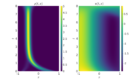
Figure 2: Evolution of the density $\rho(t,x)$ (left) and of the control $u(t,x)$ (right) up to final time $T=8$ for the Sznajd model described in Section 4.1.1 with $n=1000$ spatial discretization points and $m=200$ time steps.

Figure 3: Value of the functional $\mathcal{J}(u^{\ell})$ at the successive iterations of the steepest descent method for the Sznajd model described in Section 4.1.1 ($n=1000$ and $m=200$).

4.1.2 Hegselmann–Krause model

In the second numerical experiment we present an example of Hegselmann–Krause model for opinion formation taken from Reference [8]. In particular, we take the interaction function $p(x,y)=\chi_{\{|x-y|\leq\kappa\}}(y)$, with $\kappa=0.15$, and the target point in the running cost $x_{d}=0$. Moreover, we set the penalization parameter $\gamma=2.5$ and the diffusion coefficient $\sigma=\sqrt{0.002}$. The initial density function is

$$\rho_{0}(x)=C(0.5+\epsilon(1-x^{2})),$$

where $\epsilon=0.01$ and $C$ defined so that $\int_{\Omega}\rho_{0}(x)dx=1$. For this model, we directly present the results using a spatial discretization of $n=1000$ points and $m=100$ time steps up to the final time $T=10$. In Figure 4 we display the evolution of the density $\rho(t,x)$ and of the control $u(t,x)$. Similarly to the Sznajd model, the results match both the expectations and the outcomes in the literature. Then, we display in Figure 5 the value of the functional $\mathcal{J}(u^{\ell})$ at the successive iterations of the steepest descent method. We observe that the method needs 15 iterations to reach the input tolerance $2\cdot 10^{-3}$. Finally, this simulation takes roughly 15 seconds.

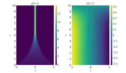
Figure 4: Evolution of the density $\rho(t,x)$ (left) and of the control $u(t,x)$ (right) up to final time $T=10$ for the Hegselmann–Krause model described in Section 4.1.2 with $n=1000$ spatial discretization points and $m=100$ time steps.

Figure 5: Value of the functional $\mathcal{J}(u^{\ell})$ at the successive iterations of the steepest descent method for the Hegselmann–Krause model described in Section 4.1.2 ($n=1000$ and $m=100$).

4.2 Crowd dynamics: fast exit scenario

In this section we consider a model for crowd dynamics taken from Reference [15]. We set the model in the spatial domain $\Omega=[-1,1]$, whose boundaries represent the exit doors. The non-local interaction kernel $p(x,y)$ is null and the selective function $s(t,x,\rho)$ is $1-\rho$ (hence, we employ the exponential Euler method (12) for the forward equation). The diffusion parameter is $\sigma=\sqrt{0.04}$ and the exit intensity flux is $\beta=10$. The initial density function models the presence of two distinct groups, namely $\rho_{0}(x)=0.9\text{e}^{-100(x+0.4)^{2}}+0.65\text{e}^{-150x^{2}}$.

Similarly to the opinion dynamics case, we first show that the expected temporal rate of convergence of the exponential integrators is preserved after a complete solution of the model. To this purpose, we discretize this problem with $n=200$ spatial discretization points and with different number of time steps, from $m=300$ to $m=700$, up to the final time $T=2$. After the stabilization of the functional $\mathcal{J}$ in the steepest descent algorithm, we measure the error at final time for $\boldsymbol{\rho}(t)$ and at initial time for $\boldsymbol{\psi}(t)$ with respect to reference solutions. We display in Figure 6 the obtained relative errors which again confirm the expected accuracy and rate of convergence.

Figure 6: Relative errors in infinity norm of $\boldsymbol{\rho}(T)$ (left, $T=2$) and $\boldsymbol{\psi}(0)$ (right), with respect to a reference solution, for the pedestrian model described in Section 4.2 with $n=200$ spatial discretization points and varying number of time steps $m$. The reference line of order 1 is also displayed.

Then, we solve the same model up to the final time $T=3$ and show its behavior. We discretize this problem with $n=1000$ spatial discretization points and $m=250$ time steps. We show the evolution of the density and of the control in Figure 7, where we can clearly see the exit of the crowd from the two doors. Moreover, we show in Figure 8 the value of the functional $\mathcal{J}(u^{\ell})$ at the successive iterations of the steepest descent method. We observe that the method needs 14 iterations to reach the input tolerance $2\cdot 10^{-3}$. Finally, the overall computational time of this simulation is about 45 seconds.

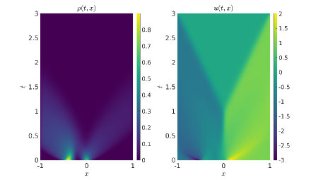
Figure 7: Evolution of the density $\rho(t,x)$ (left) and of the control $u(t,x)$ (right) up to final time $T=3$ for the two-group crowd model described in Section 4.2 with $n=1000$ spatial discretization points and $m=250$ time steps.

Figure 8: Value of the functional $\mathcal{J}(u^{\ell})$ at the successive iterations of the steepest descent method for the two-group crowd model described in Section 4.2 ($n=1000$ and $m=250$).

4.3 Mass transfer problem via optimal control

In this final example, we present an optimal control approach to a mass transfer problem, see for instance References [12, 49], where the particle density accounts for non-local interactions [13, 25]. Hence, the goal is to move the initial density function in the spatial domain $\Omega=[-1,1]$

$$\rho_{0}(x)=C(\text{e}^{-(x-\mu_{0})^{2}/(2\sigma_{0}^{2})}),$$

where $\mu_{0}=0$, $\sigma_{0}=0.1$, and $C$ is defined so that $\int_{\Omega}\rho_{0}(x)dx=1$, to a target one

$$\bar{\rho}(x)={\bar{C}}\left(\text{e}^{-(x-\mu_{1})^{2}/(2\sigma_{1}^{2})}+\text{e}^{-(x-\mu_{2})^{2}/(2\sigma_{2}^{2})}\right),$$

where $\mu_{1}=0.5$, $\sigma_{1}=0.1$, $\mu_{2}=-0.3$, and $\sigma_{2}=0.15$, and $\bar{C}$ is defined so that $\int_{\Omega}\bar{\rho}(x)dx=1$. The boundary conditions are of zero-flux type, the running cost is $e(t,x,\rho)=|\rho-\bar{\rho}|^{2}$, the interaction kernel is of Sznajd type $p(x,y)=(x^{2}-1)/20$, and the selective function is $s(t,x,\rho)=1$. The penalization parameter is $\gamma=0.1$ and the diffusion parameter is $\sigma=\sqrt{0.02}$. We discretize the problem with $n=1000$ spatial grid points and $m=200$ time steps, and we run the simulation up to the final time $T=3$. We consider a terminal cost given by $c(T,x,\rho(T,x))=\lvert\rho(T,x)-\bar{\rho}(x)\rvert^{2}$, which translates into $\psi_{T}(x)=\rho(T,x)-\bar{\rho}(x)$. In Figure 9 we plot the density functions at the initial and the final time, and we can observe that the initial density is correctly transported to the target one. In addition, in Figure 10 we present the evolution of the density and of the control. Finally, we show in Figure 11 the values of the functional $\mathcal{J}(u^{\ell})$ at the successive iterations of the steepest descent method. We observe that the method needs 33 iterations to reach the input tolerance $2\cdot 10^{-3}$, with an overall computational time of this simulation of roughly 75 seconds.

Figure 9: Density functions at initial time and at final time for the mass transfer problem described in Section 4.3 with $n=1000$ spatial discretization points and $m=200$ time steps.

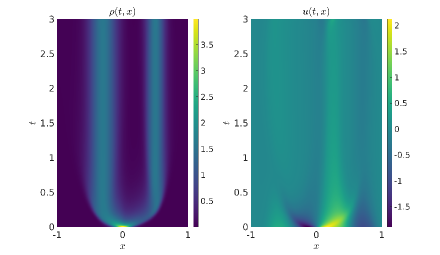
Figure 10: Evolution of the density $\rho(t,x)$ (left) and of the control $u(t,x)$ (right) up to final time $T=3$ for the mass transfer problem described in Section 4.3 with $n=1000$ spatial discretization points and $m=200$ time steps.

Figure 11: Value of the functional $\mathcal{J}(u^{\ell})$ at the successive iterations of the steepest descent method for the mass transfer problem described in Section 4.3.

5 Conclusions

We presented a mean-field optimal control model where the constraint is represented by a nonlinear PDE with non-local interaction term and diffusion describing the evolution of a continuum of agents. We provide, at a formal level, first order optimality conditions, resulting in a forward-backward coupled system with associated boundary conditions. Thus, a reduced gradient method is derived for the synthesis of the mean-field control, where the primal and adjoint equations are efficiently solved by using exponential integrators. Our proposed approach has been successfully tested on various examples from the literature, including models of opinion formation and pedestrian dynamics in the one-dimensional setting. In future works we plan to exploit the efficiency of exponential integrators to tackle higher dimensional problems (possibly using ad hoc techniques for tensor structured problems [18, 19, 20]) and scenarios where a fine spatial discretization is required to correctly capture the behavior of the controlled dynamics.

Acknowledgments

The authors were partially supported by the MIUR-PRIN Project 2017, No. 2017KKJP4X Innovative numerical methods for evolutionary partial differential equations and applications, and by RIBA 2019, No. RBVR199YFL Geometric Evolution of Multi Agent Systems.

References

- [1] Achdou, Y., Capuzzo-Dolcetta, I.: Mean Field Games: Numerical Methods. SIAM J. Numer. Anal. 48(3), 1136–1162 (2010)
- [2] Aduamoah, M., Goddard, B.D., Pearson, J.W., Roden, J.C.: Pseudospectral methods and iterative solvers for optimization problems from multiscale particle dynamics. BIT Numer. Math. 62, 1703–1743 (2022)
- [3] Al-Mohy, A.H., Higham, N.J.: A New Scaling and Squaring Algorithm for the Matrix Exponential. SIAM J. Matrix Anal. Appl. 31(3), 970–989 (2009)
- [4] Al-Mohy, A.H., Higham, N.J.: Computing the Action of the Matrix Exponential with an Application to Exponential Integrators. SIAM J. Sci. Comput. 33(2), 488–511 (2011)
- [5] Albi, G., Almi, S., Morandotti, M., Solombrino, F.: Mean-field selective optimal control via transient leadership. Appl. Math. Optim. 85(2), 1–44 (2022)
- [6] Albi, G., Bellomo, N., Fermo, L., Ha, S.Y., Kim, J., Pareschi, L., Poyato, D., Soler, J.: Vehicular traffic, crowds, and swarms: From kinetic theory and multiscale methods to applications and research perspectives. Math. Models Methods Appl. Sci. 29(10), 1901–2005 (2019)
- [7] Albi, G., Bongini, M., Cristiani, E., Kalise, D.: Invisible Control of Self-Organizing Agents Leaving Unknown Environments. SIAM J. Appl. Math. 76(4), 1683–1710 (2016)
- [8] Albi, G., Choi, Y.P., Fornasier, M., Kalise, D.: Mean Field Control Hierarchy. Appl. Math. Optim. 76, 93–135 (2017)
- [9] Albi, G., Herty, M., Pareschi, L.: Kinetic description of optimal control problems and applications to opinion consensus. Commun. Math. Sci. 13(6), 1407–1429 (2015)
- [10] Albi, G., Herty, M., Pareschi, L.: Linear multistep methods for optimal control problems and applications to hyperbolic relaxation systems. Appl. Math. Comput. 354, 460–477 (2019)
- [11] Bailo, R., Bongini, M., Carrillo, J.A., Kalise, D.: Optimal consensus control of the Cucker-Smale model. IFAC-PapersOnLine 51(13), 1–6 (2018)
- [12] Benamou, J.D., Brenier, Y.: A computational fluid mechanics solution to the Monge-Kantorovich mass transfer problem. Numer. Math. 84, 375–393 (2000)
- [13] Bongini, M., Buttazzo, G.: Optimal control problems in transport dynamics. Math. Models Methods Appl. Sci. 27(3), 427–451 (2017)
- [14] Borzì, A., Schulz, V.: Computational Optimization of Systems Governed by Partial Differential Equations. SIAM (2011)
- [15] Burger, M., Di Francesco, M., Markowich, P.A., Wolfram, M.T.: On a mean field game optimal control approach modeling fast exit scenarios in human crowds. In: 52nd IEEE Conference on Decision and Control (2013)
- [16] Burger, M., Pinnau, R., Totzeck, C., Tse, O.: Mean-Field Optimal Control and Optimality Conditions in the Space of Probability Measures. SIAM J. Control Optim. 59(2), 977–1006 (2021)
- [17] Caines, P.E., Huang, M., Malhamé, R.P.: Large population stochastic dynamic games: closed-loop McKean-Vlasov systems and the Nash certainty equivalence principle. Commun. Inf. Syst. 6(3), 221–252 (2006)
- [18] Caliari, M., Cassini, F., Einkemmer, L., Ostermann, A., Zivcovich, F.: A -mode integrator for solving evolution equations in Kronecker form. J. Comput. Phys. 455, 110989 (2022)
- [19] Caliari, M., Cassini, F., Zivcovich, F.: A -mode approach for exponential integrators: actions of -functions of Kronecker sums. arXiv preprint arXiv:2210.07667 (2022)
- [20] Caliari, M., Cassini, F., Zivcovich, F.: A -mode BLAS approach for multidimensional tensor structured problems. Numer. Algorithms (2022). Published online: 04 October 2022
- [21] Caliari, M., Cassini, F., Zivcovich, F.: BAMPHI: Matrix-free and transpose-free action of linear combinations of -functions from exponential integrators. J. Comput. Appl. Math. 423, 114973 (2023)
- [22] Caliari, M., Zivcovich, F.: On-the-fly backward error estimate for matrix exponential approximation by Taylor algorithm. J. Comput. Appl. Math. 346, 532–548 (2019)
- [23] Cannarsa, P., Capuani, R., Cardaliaguet, P.: Mean field games with state constraints: from mild to pointwise solutions of the PDE system. Calc. Var. Partial Diff. Equ. 60, 108 (2021)
- [24] Caponigro, M., Fornasier, M., Piccoli, B., Trélat, E.: Sparse stabilization and control of alignment models. Math. Models Methods Appl. Sci. 25(3), 521–564 (2015)
- [25] Carrillo, J.A., Di Francesco, M., Figalli, A., Laurent, T., Slepčev, D.: Confinement in nonlocal interaction equations. Nonlinear Anal. Theory Methods Appl. 75(2), 550–558 (2012)
- [26] Choi, Y.P., Kalise, D., Peszek, J., Peters, A.A.: A Collisionless Singular Cucker–Smale Model with Decentralized Formation Control. SIAM J. Appl. Dyn. Syst. 18(4), 1954–1981 (2019)
- [27] Cristiani, E., Piccoli, B., Tosin, A.: Multiscale Modeling of Pedestrian Dynamics, MS&A. Model. Simul. Appl., vol. 12. Springer (2014)
- [28] Cucker, F., Smale, S.: Emergent Behavior in Flocks. IEEE Trans. Automat. Control 52(5), 852–862 (2007)
- [29] Degond, P., Liu, J.G., Motsch, S., Panferov, V.: Hydrodynamic models of self-organized dynamics: Derivation and existence theory. Methods Appl. Anal. 20(2), 89–114 (2013)
- [30] D’Orsogna, M.R., Chuang, Y.L., Bertozzi, A.L., Chayes, L.S.: Self-Propelled Particles with Soft-Core Interactions: Patterns, Stability, and Collapse. Phys. Rev. Lett. 96(10), 104302 (2006)
- [31] Dyer, J.R.G., Johansson, A., Helbing, D., Couzin, I.D., Krause, J.: Leadership, consensus decision making and collective behaviour in humans. Philos. Trans. R. Soc. Lond., B, Biol. Sci. 364(1518), 781–789 (2009)
- [32] Fornasier, M., Piccoli, B., Rossi, F.: Mean-field sparse optimal control. Philos. Trans. R. Soc. Lond., A, Math. Phys. Eng. Sci. 372(2028), 20130400 (2014)
- [33] Fornasier, M., Solombrino, F.: Mean-Field Optimal Control. ESAIM Control Optim. Calc. Var. 20(4), 1123–1152 (2014)
- [34] Freudenthaler, G., Meurer, T.: PDE-based multi-agent formation control using flatness and backstepping: Analysis, design and robot experiments. Automatica 115, 108897 (2020)
- [35] Gaudreault, S., Rainwater, G., Tokman, M.: KIOPS: A fast adaptive Krylov subspace solver for exponential integrators. J. Comput. Phys. 372, 236–255 (2018)
- [36] Gómez-Serrano, J., Graham, C., Le Boudec, J.Y.: The bounded confidence model of opinion dynamics. Math. Models Methods Appl. Sci. 22(2), 1150007 (2012)
- [37] Hager, W.W.: Runge-Kutta methods in optimal control and the transformed adjoint system. Numer. Math. 87, 247–282 (2000)
- [38] Hegselmann, R., Krause, U.: Opinion dynamics and bounded confidence models, analysis, and simulation. JASSS 5(3) (2002)
- [39] Herty, M., Pareschi, L.: Fokker-Planck asymptotics for traffic flow models. Kinet. Relat. Models 3(1), 165–179 (2010)
- [40] Herty, M., Pareschi, L., Steffensen, S.: Implicit-Explicit Runge–Kutta Schemes for Numerical Discretization of Optimal Control Problems. SIAM J. Numer. Anal. 51(4), 1875–1899 (2013)
- [41] Hochbruck, M., Ostermann, A.: Exponential integrators. Acta Numer. 19, 209–286 (2010)
- [42] Lasry, J.M., Lions, P.L.: Mean field games. Japanese J. Math. 2, 229–260 (2007)
- [43] Luan, V.T., Pudykiewicz, J.A., Reynolds, D.R.: Further development of efficient and accurate time integration schemes for meteorological models. J. Comput. Phys. 376, 817–837 (2019)
- [44] Motsch, S., Tadmor, E.: Heterophilious Dynamics Enhances Consensus. SIAM Rev. 56(4), 577–621 (2014)
- [45] Oh, K.K., Park, M.C., Ahn, H.S.: A survey of multi-agent formation control. Automatica 53, 424–440 (2015)
- [46] Peters, A.A., Middleton, R.H., Mason, O.: Leader tracking in homogeneous vehicle platoons with broadcast delays. Automatica 50(1), 64–74 (2014)
- [47] Piccoli, B., Tosin, A.: Pedestrian flows in bounded domains with obstacles. Contin. Mech. Thermodyn. 21(2), 85–107 (2009)
- [48] Saad, Y.: Analysis of Some Krylov Subspace Approximations to the Matrix Exponential Operator. SIAM J. Numer. Anal. 29(1), 209–228 (1992)
- [49] Santambrogio, F.: Optimal Transport for Applied Mathematicians, Progress in Nonlinear Differential Equations and Their Applications, vol. 87. Birkäuser (2015)
- [50] Sastre, J., Ibáñez, J., Defez, E.: Boosting the computation of the matrix exponential. Appl. Math. Comput. 340, 206–220 (2019)
- [51] Skaflestad, B., Wright, W.M.: The scaling and modified squaring method for matrix functions related to the exponential. Appl. Numer. Math. 59(3–4), 783–799 (2009)
- [52] Sznajd-Weron, K., Sznajd, J.: Opinion evolution in closed community. Int. J. of Mod. Phys. C 11(6), 1157–1165 (2000)
- [53] Toscani, G.: Kinetic models of opinion formation. Commun. Math. Sci. 4(3), 481–496 (2006)