Anisotropic stars made of exotic matter within the complexity factor formalism

Abstract

We investigate exotic stars composed of dark energy within the context of Einstein’s General Relativity, by applying an extended Chaplygin gas equation-of-state. To account for anisotropies, we utilize a formalism based on the complexity factor to obtain numerical solutions. By applying well-established criteria, we demonstrate that the solutions are physically valid and well-behaved. In addition, a comparison with a more conventional approach is also conducted.

1 Introduction

Any reasonable modern cosmological model must include Dark Energy (DE). Nevertheless, the nature and origin of Dark Energy remain a mystery despite its fundamental importance in modern theoretical cosmology SupernovaSearchTeam:1998fmf ; SupernovaCosmologyProject:1998vns ; Freedman:2003ys . As it is well known, a cosmological model made of only matter and radiation cannot lead to accelerated solutions to the universe as predicted by Einstein’s Theory of General Relativity (GR) Einstein:1916vd . This kind of solution is obtained by including a constant $\Lambda$ in Einstein’s field equations Einstein:1917ce , i.e., by adding the contribution of the dark energy. Despite its simplicity, such accelerated cosmological model is in exceptional agreement with a vast amount of observational data. Such a cosmological model is known as the concordance cosmological model or the $\Lambda$CDM model. Nevertheless, $\Lambda$ suffers from the cosmological constant ongoing problem Weinberg:1988cp ; Zeldovich:1967gd . Additionally, this $\Lambda$–problem is amplified by the current values estimation of the Hubble constant $H_{0}$, using high red-shift CMB data and local measurements at low red-shift data, e.g., Ryden:2017dxw ; Colin:2019opb ; Verde:2013wza ; Bolejko:2017fos . In fact, the value of the $H_{0}$ computed by the PLANCK Collaboration Planck:2015fie ; Planck:2018vyg , $H_{0}=(67-68)~{}km/(Mpc\>sec)$, is lower than the value estimated from local measurements Riess:2016jrr ; Riess:2018byc , $H_{0}=(73-74)~{}km/(Mpc\>sec)$. This $H_{0}$ tension points to a cosmological model with new physics Mortsell:2018mfj ; Kazantzidis:2018rnb ; Gannouji:2018ncm ; Alvarez:2020xmk .

Over the years, this incomplete picture of the cosmological concordance model has motivated the arrival of many new and alternative models. We can classify recent DE cosmological models into two generic categories: (i) alternative theories of gravity for which the solutions have additional corrective terms compared to the standard case; (ii) by employing a new dynamical degree of freedom by means of a convenient equation-of-state. In the first class of models, one finds, for instance, Scalar-Tensor theories of gravity Brans:1961sx ; Brans:1962zz ; Sanchez:2010ng ; Panotopoulos:2017clp , brane-world models Randall:1999ee ; Randall:1999vf ; Dvali:2000hr ; Langlois:2002bb ; Maartens:2003tw and f(R) theories of gravity Sotiriou:2008rp ; DeFelice:2010aj ; Hu:2007nk ; Starobinsky:2007hu ; and for the second class, one finds models such as k-essence Armendariz-Picon:2000ulo , phantom Arefeva:2004odl , quintessence Ratra:1987rm , quintom Lazkoz:2006pa , or tachyonic Bagla:2002yn . For a good review article on the dynamics of dark energy see for instance Copeland:2006wr .

In this work, we will focus our study on the generalized Chaplying gas equation-of-state Szydlowski:2020ilx , widely used in many cosmological model extensions. Here, we study the properties of relativistic astrophysical objects, where we opt to use the same equation of state.

In studies of compact relativistic astrophysical objects the authors usually focus on stars made of an isotropic fluid, where the radial pressure $P_{r}$ equals the tangential pressure $P_{\bot}$. However, celestial bodies are not always made of isotropic fluid only. In fact under certain conditions the fluid can become anisotropic. The review article of Ruderman Ruderman:1972aj mentioned for the first time such a possibility: this author makes the observation that relativistic particle interactions in a very dense nuclear matter medium could lead to the formation of anisotropies. The study on anisotropies in relativistic stars has received a boost by the subsequent work of Bowers:1974tgi . Interestingly, Ivanov 2010IJTP…49.1236I has shown that by considering a compact object to be an anisotropic star, the effects of shear, electromagnetic field, etc, can be automatically taken into account. Indeed, anisotropies can arise in many scenarios of a dense matter medium, like phase transitions Sokolov:1998er , pion condensation Sawyer:1972cq , or in presence of type 3A super-fluid Kippenhahn:2012qhp . See also MakANDHarko ; Deb:2016lvi ; Deb:2015vda for more recent works on the topic, and references therein. In these works relativistic models of anisotropic quark stars were studied, and the energy conditions were fulfilled. In particular, in MakANDHarko an exact analytical solution was obtained, in Deb:2016lvi an attempt was made to find a singularity free solution to Einstein’s field equations, and in Deb:2015vda the Homotopy Perturbation Method was employed, which is a tool that facilitates to tackle Einstein’s field equations. What is more, alternative approaches have been considered to incorporate anisotropies into known isotropic solutions Gabbanelli:2018bhs ; Ovalle:2017fgl ; Ovalle:2017wqi .

Beyond the collisionless dark matter paradigm, self-interacting dark matter has been proposed as an attractive solution to the dark matter crisis at galactic scales Tulin:2017ara . In this scenario one can imagine relativistic stars made entirely of self-interacting dark matter, see e.g. Li:2012sg ; Maselli:2017vfi ; Panotopoulos:2018enj . In a similar way, given that the current cosmic acceleration calls for dark energy, very recently a couple of works appeared in the literature, where the authors entertain the possibility that stars made of dark energy or more generically exotic matter just might exist NewtonSingh:2020rsk ; Tello-Ortiz:2020svg .

These exotic stars are unique objects like any other compact object that manifest themselves across many multi-messenger signals like gravitational waves, neutrinos, cosmic rays and electromagnetic radiation from radio up to gamma-rays. For instance, we will be able to test many of these stellar models using the data from the present and next generation of gravitational wave detectors such as LIGO, Virgo, KAGRA and LISA.

In the present work, we propose to study non-rotating dark energy stars with anisotropic matter assuming a generalized equation-of-state of the form $p=-B^{2}/\rho+A^{2}\rho$ (with $A$ and $B$ being constants). A simplified version of this, known as a Chaplygin equation-of-state, was introduced in Cosmology long time ago to unify the description of non-relativistic matter and the cosmological constant Kamenshchik:2001cp ; Bento:2002ps ; Debnath:2004cd . Such a generic equation-of-state is originated by a viscose matter, that when considered in a cosmological context gives rise to the unification of dark matter and dark energy Szydlowski:2020ilx .

2 Relativistic spheres within GR

We will consider a static, spherically symmetric object (static fluid), and we will assume locally certain anisotropy, bounded by a spherical surface $\Sigma$. The line element considering Schwarzschild–like coordinates is written as

$$ds^{2}=e^{\nu}dt^{2}-e^{\lambda}dr^{2}-r^{2}d\Omega^{2},$$ (1)

where $\nu(r)$ and $\lambda(r)$ are, as always, the corresponding metric potential, depending on the radial coordinate only, and $d\Omega^{2}\equiv\left(d\theta^{2}+\sin^{2}\theta d\phi^{2}\right)$ correspond to the element of solid angle. We will take: $x^{0}=t;\,x^{1}=r;\,x^{2}=\theta;\,x^{3}=\phi$. The classical Einstein field equations with a vanishing cosmological constant are given by

$$G^{\nu}_{\mu}=8\pi GT^{\nu}_{\mu},$$ (2)

where $G$ is Newton’s constant ($G=1$) and $T^{\nu}_{\mu}$ is the energy-momentum tensor. In the comoving frame, the matter content is described by an anisotropic fluid with energy density $\rho$, radial pressure $P_{r}$, and tangential pressure $P_{\bot}$. The covariant energy-momentum tensor can be expressed in local Minkowski coordinates as $T^{\mu}_{\nu}=\{\rho,P_{r},P_{\bot},P_{\bot}\}$, and the resulting field equations take the form:

$$\rho = -\frac{1}{8\pi}\left[-\frac{1}{r^{2}}+e^{-\lambda}\left(\frac{1}{r^{2}}-\frac{\lambda^{\prime}}{r}\right)\right],$$ (3)

$$P_{r} = -\frac{1}{8\pi}\left[\frac{1}{r^{2}}-e^{-\lambda}\left(\frac{1}{r^{2}}+\frac{\nu^{\prime}}{r}\right)\right],$$ (4)

$$P_{\bot} = \frac{1}{32\pi}e^{-\lambda}\left(2\nu^{\prime\prime}+\nu^{\prime 2}-\lambda^{\prime}\nu^{\prime}+2\frac{\nu^{\prime}-\lambda^{\prime}}{r}\right),$$ (5)

where the derivatives with respect to $r$ are denoted by primes.

As it is well known, we can combine the last equations to produce the hydrostatic equilibrium equation (also known as the generalized Tolman-Opphenheimer-Volkoff equation), i.e.,

$$-\frac{1}{2}\nu^{\prime}\left(\rho+P_{r}\right)-P^{\prime}_{r}+\frac{2}{r}\left(P_{\bot}-P_{r}\right)=0.$$ (6)

We can express the equilibrium equation as a balance between three forces, namely the gravitational force ($F_{g}$), hydrostatic force ($F_{r}$), and anisotropic force ($F_{p}$), which we define as follows for convenience:

$$F_{g}=-\frac{\nu^{\prime}\left(\rho+P_{r}\right)}{2},\;F_{r}=-P^{\prime}_{r}\;{\rm and}\;F_{p}=\frac{2\Pi}{r}.$$ (7)

where $\Delta\equiv\Pi=P_{\bot}-P_{r}$. Thus, equation (6) can now be expressed as:

$$F_{g}+F_{r}+F_{p}=0.$$ (8)

The equilibrium for a compact star is maintained by the balance of three forces, as established by the previous equation (8) Prasad:2021eju . It is noteworthy that if $F_{p}$ is equal to zero, then the standard TOV equation is obtained. When $P_{\bot}>P_{r}$ (or $\Pi>0$), $F_{p}>0$ generates a repulsive force in equation (8) that counteracts the attractive forces of $F_{g}$ and $F_{r}$. Conversely, when $P_{\bot}<P_{r}$ (or $\Pi<0$), $F_{p}<0$ becomes an additional attractive force that acts in conjunction with the other forces. Alternatively, we can remove the $\nu^{\prime}$-dependence in equation (6) to obtain a more convenient equation, namely

$$P^{\prime}_{r}=-\frac{(m+4\pi P_{r}r^{3})}{r\left(r-2m\right)}\left(\rho+P_{r}\right)+\frac{2}{r}\left(P_{\bot}-P_{r}\right),$$ (9)

To do that, we have used the relation

$$\frac{1}{2}\nu^{\prime}=\frac{m+4\pi P_{r}r^{3}}{r\left(r-2m\right)},$$ (10)

Furthermore, the mass function $m$ is obtained by:

$$R^{3}_{232}=1-e^{-\lambda}=\frac{2m}{r},$$ (11)

or,

$$m=4\pi\int^{r}_{0}\tilde{r}^{2}\rho\ d\tilde{r}.$$ (12)

Now, let us rewrite the energy-momentum tensor as follow

$$T^{\mu}_{\nu}=\rho u^{\mu}u_{\nu}-Ph^{\mu}_{\nu}+\Pi^{\mu}_{\nu},$$ (13)

Firstly, we set the four-velocity as $u^{\mu}=(e^{-\frac{\nu}{2}},0,0,0)$, and the four acceleration, $a^{\alpha}=u^{\alpha}_{;\beta}u^{\beta}$, whose any non–vanishing component is $a_{1}=-\nu^{\prime}/2$. Subsequently, the set $\{\Pi^{\mu}_{\nu},\Pi,h^{\mu}_{\nu},s^{\mu},P\}$ is taken according to

$$\Pi^{\mu}_{\nu} = \Pi\bigg{(}s^{\mu}s_{\nu}+\frac{1}{3}h^{\mu}_{\nu}\bigg{)}$$ (14)

$$\Pi = P_{\bot}-P_{r}$$ (15)

$$h^{\mu}_{\nu} = \delta^{\mu}_{\nu}-u^{\mu}u_{\nu}$$ (16)

$$s^{\mu} = (0,e^{-\frac{\lambda}{2}},0,0)$$ (17)

$$P \equiv \frac{1}{3}\Bigl{(}P_{r}+2P_{\bot}\Bigl{)}$$ (18)

with the properties $s^{\mu}u_{\mu}=0$, $s^{\mu}s_{\mu}=-1$. To obtain the exterior solution, we match the problem with the Schwarzschild spacetime, as follows:

$$ds^{2}=\left(1-\frac{2M}{r}\right)dt^{2}-\left(1-\frac{2M}{r}\right)^{-1}dr^{2}-r^{2}d\Omega^{2}.$$ (19)

The problem should be supplemented using certain boundary conditions on the surface $r=\text{constant}=R$, with $R$ being the radius of the star. Therefore, we require that the first and second fundamental forms are continuous across that surface. This condition implies that:

$$e^{\nu_{\Sigma}} = 1-\frac{2M}{R},$$ (20)

$$e^{-\lambda_{\Sigma}} = 1-\frac{2M}{R},$$ (21)

$$\left[P_{r}\right]_{\Sigma} = 0.$$ (22)

Here, the subscript $\Sigma$ indicates that the quantity is evaluated on the boundary surface $\Sigma$. In conclusion, it is worth noting that the last three equations are both necessary and sufficient conditions for a smooth matching of the two metrics (1) and (19) on the surface $\Sigma$.

3 Anisotropic matter: Complexity factor

In what follows, we will briefly summarize the underlying physics behind the definition of the complexity factor, focusing on the astrophysical relevance of such quantity. Let us first start mentioning the seminal paper by Herrera Herrera:2018bww , where a new and non-trivial way to reveal when static self-gravitating objects are anisotropic was properly introduced. Furthermore, this revised definition aims to address two issues that were identified in earlier attempts to define complexity. The first problem appears when the probability distribution (which appear in the definition of “disequilibrium” and information) is replaced by the energy density of the fluid distribution Sanudo:2008bu . The second issue arises from the recognition that previous definitions of complexity only take into account the energy density of the fluid, while neglecting other crucial components such as pressure. Thus, the new definition introduced by L.H. try to make progress by fixing the above mentioned issues.

Originally, the new definition of the complexity factor was investigated only under a mathematical point of view (see Sharif:2018pgq ; Sharif:2018efi ; Abbas:2018cha ; Herrera:2019cbx and references therein). However, the real value of such definition becomes evident when we use it as a supplementary condition to close the set of differential equations of a self-gravitational system. Additionally, the complexity factor may serve as a self-consistent method for integrating anisotropies Arias:2022qrm ; Andrade:2021flq , which has been explored in recent studies Maurya:2022yva ; Maurya:2022cyv ; Sharif:2022akn ; Sharif:2022sad ; Govender:2022ome ; Bogadi:2022yqb ; Bargueno:2022yob ; Sadiq:2022uwj and their associated references.

As was previously pointed out, the complexity factor appears in the orthogonal splitting of the Riemann tensor for static self-gravitating fluids with spherical symmetry, and for a detailed step-by-step computation, we should see the original paper Herrera:2018bww and also Gomez-Lobo:2007mbg . Therefore, while we will refrain from delving deeply into the orthogonal decomposition of the Riemann tensor, we must still establish the following quantities:

$$Y_{\alpha\beta} = R_{\alpha\gamma\beta\delta}u^{\gamma}u^{\delta},$$ (23)

$$Z_{\alpha\beta} = R^{*}_{\alpha\gamma\beta\delta}u^{\gamma}u^{\delta}=\frac{1}{2}\eta_{\alpha\gamma\epsilon\mu}R^{\epsilon\mu}_{\quad\beta\delta}u^{\gamma}u^{\delta},$$ (24)

$$X_{\alpha\beta} = R^{*}_{\alpha\gamma\beta\delta}u^{\gamma}u^{\delta}=\frac{1}{2}\eta_{\alpha\gamma}^{\quad\epsilon\mu}R^{*}_{\epsilon\mu\beta\delta}u^{\gamma}u^{\delta},$$ (25)

Please, notice that the symbol $*$ represent the dual tensor, namely

$$R^{*}_{\alpha\beta\gamma\delta}=\frac{1}{2}\eta_{\epsilon\mu\gamma\delta}R_{\alpha\beta}^{\quad\epsilon\mu}$$ (26)

and $\eta_{\epsilon\mu\gamma\delta}$ is the well-known Levi-Civita tensor. Taking advantage of the decomposition of the Riemann tensor, we rewrite the set of scalars $\{Y_{\alpha\beta},Z_{\alpha\beta},X_{\alpha\beta}\}$ in term of the physical variables, i.e.,

$$Y_{\alpha\beta} = \frac{4\pi}{3}(\rho+3P)h_{\alpha\beta}+4\pi\Pi_{\alpha\beta}+E_{\alpha\beta},$$ (27)

$$Z_{\alpha\beta} = 0,$$ (28)

$$X_{\alpha\beta} = \frac{8\pi}{3}\rho h_{\alpha\beta}+4\pi\Pi_{\alpha\beta}-E_{\alpha\beta}.$$ (29)

Notice that the corresponding tensor $E_{\alpha\beta}$ (defined as $E_{\alpha\beta}=C_{\alpha\gamma\beta\delta}u^{\gamma}u^{\delta}$) is given by

$$E_{\alpha\beta}=E\bigg{(}s_{\alpha}s_{\beta}+\frac{1}{3}h_{\alpha\beta}\bigg{)},$$ (30)

with

$$E=-\frac{e^{-\lambda}}{4}\left[\nu^{\prime\prime}+\frac{{\nu^{\prime}}^{2}-\lambda^{\prime}\nu^{\prime}}{2}-\frac{\nu^{\prime}-\lambda^{\prime}}{r}+\frac{2(1-e^{\lambda})}{r^{2}}\right],.$$ (31)

The following properties must be satisfied:

$$E^{\alpha}_{\,\,\alpha}=0,\quad E_{\alpha\gamma}=E_{(\alpha\gamma)},\quad E_{\alpha\gamma}u^{\gamma}=0.$$ (32)

Even more, as was also demonstrated by Herrera:2009zp , the tensors $\{Y_{\alpha\beta},Z_{\alpha\beta},X_{\alpha\beta}\}$ can be represented in term of alternative scalar functions. Considering the tensors $X_{\alpha\beta}$ and $Y_{\alpha\beta}$ in the static case, the so-called structure scalars $X_{T},X_{TF},Y_{T},Y_{TF}$ can be written in term of the physical variables as follow:

$$X_{T} = 8\pi\rho,$$ (33)

$$X_{TF} = \frac{4\pi}{r^{3}}\int^{r}_{0}{\tilde{r}^{3}\rho^{\prime}d\tilde{r}},$$ (34)

$$Y_{T} = 4\pi(\rho+3P_{r}-2\Pi),$$ (35)

$$Y_{TF} = 8\pi\Pi-\frac{4\pi}{r^{3}}\int^{r}_{0}{\tilde{r}^{3}\rho^{\prime}d\tilde{r}}.$$ (36)

From Eqs.(34)-(36), the local anisotropy of pressure is determined by $X_{TF}$ and $Y_{TF}$ via the following relation:

$$8\pi\Pi=X_{TF}+Y_{TF}.$$ (37)

When the complexity vanishes ($Y_{TF}=0$), it implies the following relation between the energy density and the anisotropic factor:

$$\Pi(r)=\frac{1}{2r^{3}}\>\int^{r}_{0}{\tilde{r}^{3}\rho^{\prime}(\tilde{r})d\tilde{r}}.$$ (38)

The last condition has also been significantly investigated along years introducing, via alternative ansatzs, several concrete forms of the anisotropy $\Pi\equiv P_{\perp}-P_{r}$ and different equations of state (see for instance Panotopoulos:2018joc ; Panotopoulos:2018ipq ; Moraes:2021lhh ; Gabbanelli:2018bhs ; Panotopoulos:2019wsy ; Lopes:2019psm ; Panotopoulos:2019zxv ; Abellan:2020jjl ; Panotopoulos:2020zqa ; Bhar:2020ukr ; Panotopoulos:2020kgl ; Panotopoulos:2021obe ; Panotopoulos:2021dtu and references therein). Given that a profound comprehension of the idea of complexity is still under construction, the connection between $\Pi$ (or more precisely, any equation of state $P_{\bot}\equiv P_{\bot}(\rho)$) and the definition of complexity factor $Y_{TF}$ is still missing.

4 Discussion

This work examines anisotropic stars composed of exotic matter through the well-established complexity formalism. Our study focuses on numerically computing solutions for a realistic compact distribution of matter, and comparing these results with those obtained using the conventional formalism within the framework of GR. To this end, we employ a generalized Chaplyin equation-of-state to close the system. In the figures presented, we show the evolution of several key quantities of the star. Notably, we observe that:

1. The mass function increases, while the anisotropic factor, energy density, and pressures decrease throughout the star.

2. The speed of sound, both radial and tangential, increases and decreases, respectively, with both values lower than $c_{0}^{2}\equiv 1$, the relativistic adiabatic index, while $\Gamma(r)$ increases and remains greater than $\Gamma_{0}\equiv 4/3$.

3. Furthermore, the corresponding energy conditions are satisfied.

Therefore, based on these numerical results, we can confidently assert that the complexity factor formalism is a robust approach for obtaining well-defined solutions within the context of compact stars.

As a supplementary check, we obtained interior solutions using a more standard approach. This involved adding external constraints to close the system of differential equations, and we employed numerical methods to carry out the calculations. As a toy model, we considered an anisotropic factor, $\Pi(r)$, defined by the equation

$$\Pi(r)=-\bigg{(}\frac{r}{a}\bigg{)}^{2}\rho(r),$$ (39)

where $a$ is a dimensionful parameter with units of length. This parameter encodes the strength of the anisotropy.

The anisotropic factor used in Moraes:2021lhh has a simple mathematical form that satisfies fundamental requirements: it has the correct dimensions, is negative, and vanishes at the star’s center ($\Pi(r=0)=0$). To further explore its behavior, we investigate two scenarios characterized by large ($a_{\text{large}}=30~{}\text{km}$) and small ($a_{\text{small}}=10~{}\text{km}$) values of $a$.

Although it is not necessary, one can derive the differential equation

$$\Pi^{\prime}(r)=\frac{2}{r}\Pi(r)-\frac{r^{2}}{a^{2}}\rho^{\prime}(r),$$ (40)

from the anisotropic factor ansatz given above. This equation bears a striking resemblance to the differential equation

$$\Pi^{\prime}(r)=-\frac{3}{r}\Pi(r)+\frac{\rho^{\prime}(r)}{2},$$ (41)

which is obtained using equation (36) and the condition that the complexity vanishes, i.e., $Y_{TF}=0$. Equation (41) can be straightforwardly derived as follows: We first take the derivative of both sides of equation (39) with respect to $r$ and obtain

$$\Pi^{\prime}(r)=\frac{1}{a^{2}}[2r\rho+r^{2}\rho^{\prime}(r)].$$ (42)

We then use the anisotropic factor definition again,

$$\frac{\Pi(r)}{r}=-\frac{r}{a^{2}}\rho(r).$$ (43)

Our main finding is that when the normalized anisotropy, $\Pi(r)/B$, is comparable to the one studied within the complexity factor formalism, the resulting solution violates causality, as shown in Fig. 4 for the small $a$ case. On the other hand, if the solution is realistic and meets all the criteria, the star’s anisotropy is much lower, as illustrated in Fig. 5 for the large $a$ case, while retaining a similar mass.

We illustrate the mass-to-radius profiles for three models in Fig. 6. The left panel shows the models within the complexity factor formalism, while the right panel presents a more standard approach for the case of large $a$. The three models are:

$$A=\sqrt{0.4},\;\;\;\;\;B=0.23\times 10^{-3}km^{-2}$$ (44)

for Model 1,

$$A=\sqrt{0.425},\;\;\;\;\;B=0.215\times 10^{-3}km^{-2}$$ (45)

for Model 2, and

$$A=\sqrt{0.45},\;\;\;\;\;B=0.2\times 10^{-3}km^{-2}$$ (46)

for Model 3.

The curves show that the star’s radius first reaches a maximum value, followed by the maximum mass of the star. The complexity factor formalism predicts smaller and lighter objects compared to the conventional approach, despite both cases having a negative anisotropic factor. The complexity factor is an effective method to include modifications in the structure of compact stars resulting from anisotropy. This leads to alterations in the TOV equations for such stars, balancing three forces: gravity, hydrostatic and anisotropic forces.

In the final figure (Fig. 7), we present the mass-to-radius relationships for isotropic and anisotropic stars using both approaches for Model 1. We begin by plotting the M-R profile for stars composed of isotropic matter (dashed line), and then explore anisotropies within the vanishing complexity formalism, yielding the cyan curve. Turning to the conventional method, we can examine the impact of the continuous parameter characterizing the ansatz for the anisotropic factor on the profiles, which are shown in the other three curves in the figure. As the anisotropy increases, the profile gradually shifts towards the one corresponding to complexity. However, at a certain point, the violation of causality occurs, marking the upper limit for the anisotropic factor using the conventional method. This critical point signifies where the solution becomes unrealistic or unviable, and it is crucial to halt the analysis to ensure the solution’s physical validity. As a result, the last permitted profile differs significantly from the one obtained using complexity.

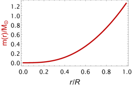
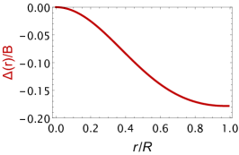
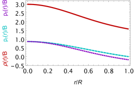
Figure 1: The left panel shows the mass function in solar masses, the middle panel displays the anisotropic factor, and the right panel illustrates the energy density and pressures as a function of the radial coordinate throughout the star, specifically for anisotropic DE stars within the complexity factor.

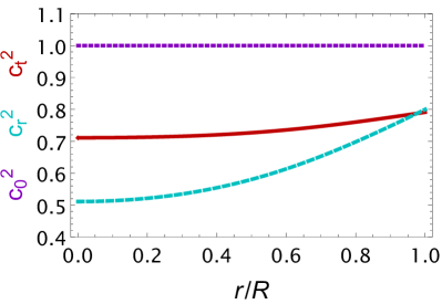
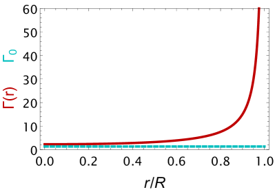
Figure 2: The left panel displays the speed of sounds, while the right panel exhibits the relativistic adiabatic index as a function of the radial coordinate throughout the anisotropic DE stars.

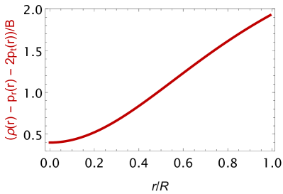
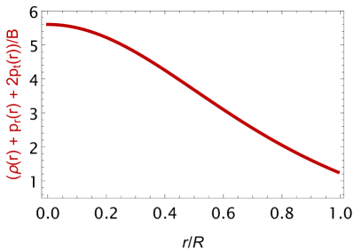
Figure 3: The energy conditions for anisotropic DE stars within the complexity factor are presented as a function of the radial coordinate throughout the star.

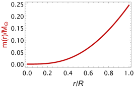
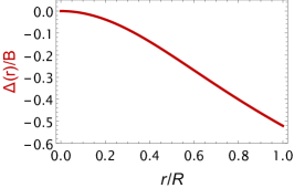
Figure 4: Anisotropic DE stars using a standard approach and assuming a small value for $a$: the left panel of the figure shows the mass function in solar masses, the middle panel shows the anisotropic factor, and the right panel shows the sound speeds, all plotted as a function of the radial coordinate throughout the star.

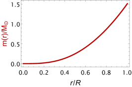
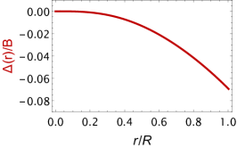
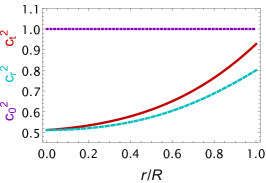
Figure 5: Anisotropic DE stars using a standard approach and assuming a large value for $a$: the figure displays the mass function in solar masses in the left panel, the anisotropic factor in the middle panel, and the sound speed in the right panel, all plotted as a function of the radial coordinate throughout the star.

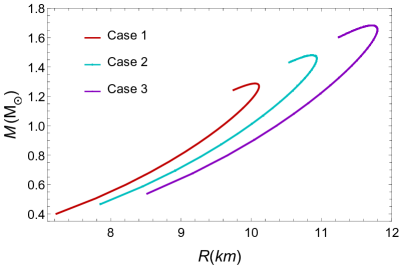
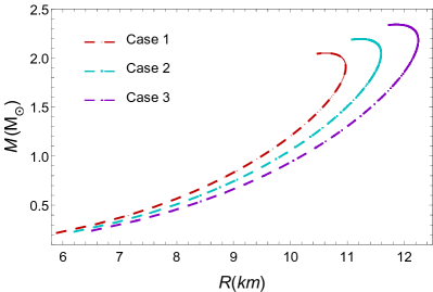
Figure 6: The mass-to-radius profiles for two alternative approaches: the left panel shows the profiles for three models corresponding to the curves following the complexity formalism, while the right panel shows the profiles for three models corresponding to curves obtained in the conventional scenario.

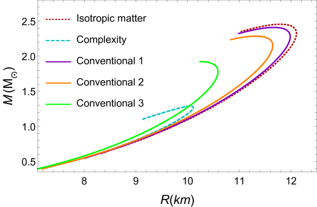
Figure 7: The mass-to-radius profiles for Model 1 in different cases: the dashed curve represents the profile when considering isotropic matter; the cyan curve corresponds to utilizing the vanishing complexity factor formalism; and the three curves in between depict the conventional method for values of $a$ equal to $100\,km$ (less anisotropic), $50\,km$ (moderate anisotropy), and $25\,km$ (more anisotropic).

5 Conclusions

To summarize our work, we have obtained interior solutions of exotic stars made of dark energy, taking into account the presence of anisotropies and adopting the extended Chaplygin gas equation-of-state. The anisotropic factor is treated employing the formalism based on the complexity factor, and the structure equations have been integrated numerically. The solutions are shown to be well-behaved and realistic. Moreover, we have made a comparison with another more conventional approach, where the form of the anisotropic factor is introduced by hand.

6 Acknowledgments

A. R. is funded by the María Zambrano contract ZAMBRANO 21-25 (Spain). I. L. thanks the Fundação para a Ciência e Tecnologia (FCT), Portugal, for the financial support to the Center for Astrophysics and Gravitation (CENTRA/IST/ULisboa) through the Grant Project No.
 UIDB/00099/2020 and Grant No. PTDC/FIS-AST/28920
/2017.

References

- [1] Adam G. Riess et al. Observational evidence from supernovae for an accelerating universe and a cosmological constant. Astron. J., 116:1009–1038, 1998.
- [2] S. Perlmutter et al. Measurements of and from 42 high redshift supernovae. Astrophys. J., 517:565–586, 1999.
- [3] Wendy L. Freedman and Michael S. Turner. Measuring and understanding the universe. Rev. Mod. Phys., 75:1433–1447, 2003.
- [4] Albert Einstein. The Foundation of the General Theory of Relativity. Annalen Phys., 49(7):769–822, 1916.
- [5] Albert Einstein. Cosmological Considerations in the General Theory of Relativity. Sitzungsber. Preuss. Akad. Wiss. Berlin (Math. Phys. ), 1917:142–152, 1917.
- [6] Steven Weinberg. The Cosmological Constant Problem. Rev. Mod. Phys., 61:1–23, 1989.
- [7] Y. B. Zeldovich. Cosmological Constant and Elementary Particles. JETP Lett., 6:316, 1967.
- [8] Barbara Ryden. A constant conflict. Nature Phys., 13(3):314–314, 2017.
- [9] Jacques Colin, Roya Mohayaee, Mohamed Rameez, and Subir Sarkar. Evidence for anisotropy of cosmic acceleration. Astron. Astrophys., 631:L13, 2019.
- [10] Licia Verde, Pavlos Protopapas, and Raul Jimenez. Planck and the local Universe: Quantifying the tension. Phys. Dark Univ., 2:166–175, 2013.
- [11] Krzysztof Bolejko. Emerging spatial curvature can resolve the tension between high-redshift CMB and low-redshift distance ladder measurements of the Hubble constant. Phys. Rev. D, 97(10):103529, 2018.
- [12] P. A. R. Ade et al. Planck 2015 results. XIII. Cosmological parameters. Astron. Astrophys., 594:A13, 2016.
- [13] N. Aghanim et al. Planck 2018 results. VI. Cosmological parameters. Astron. Astrophys., 641:A6, 2020. [Erratum: Astron.Astrophys. 652, C4 (2021)].
- [14] Adam G. Riess et al. A 2.4% Determination of the Local Value of the Hubble Constant. Astrophys. J., 826(1):56, 2016.
- [15] Adam G. Riess et al. Milky Way Cepheid Standards for Measuring Cosmic Distances and Application to Gaia DR2: Implications for the Hubble Constant. Astrophys. J., 861(2):126, 2018.
- [16] Edvard Mörtsell and Suhail Dhawan. Does the Hubble constant tension call for new physics? JCAP, 09:025, 2018.
- [17] Lavrentios Kazantzidis and Leandros Perivolaropoulos. Evolution of the tension with the Planck15/CDM determination and implications for modified gravity theories. Phys. Rev. D, 97(10):103503, 2018.
- [18] Radouane Gannouji, Lavrentios Kazantzidis, Leandros Perivolaropoulos, and David Polarski. Consistency of modified gravity with a decreasing in a CDM background. Phys. Rev. D, 98(10):104044, 2018.
- [19] Pedro D. Alvarez, Benjamin Koch, Cristobal Laporte, and Ángel Rincón. Can scale-dependent cosmology alleviate the tension? JCAP, 06:019, 2021.
- [20] C. Brans and R. H. Dicke. Mach’s principle and a relativistic theory of gravitation. Phys. Rev., 124:925–935, 1961.
- [21] C. H. Brans. Mach’s Principle and a Relativistic Theory of Gravitation. II. Phys. Rev., 125:2194–2201, 1962.
- [22] J. C. Bueno Sanchez and L. Perivolaropoulos. Evolution of Dark Energy Perturbations in Scalar-Tensor Cosmologies. Phys. Rev. D, 81:103505, 2010.
- [23] Grigoris Panotopoulos and Ángel Rincón. Stability of cosmic structures in scalar–tensor theories of gravity. Eur. Phys. J. C, 78(1):40, 2018.
- [24] Lisa Randall and Raman Sundrum. A Large mass hierarchy from a small extra dimension. Phys. Rev. Lett., 83:3370–3373, 1999.
- [25] Lisa Randall and Raman Sundrum. An Alternative to compactification. Phys. Rev. Lett., 83:4690–4693, 1999.
- [26] G. R. Dvali, Gregory Gabadadze, and Massimo Porrati. 4-D gravity on a brane in 5-D Minkowski space. Phys. Lett. B, 485:208–214, 2000.
- [27] David Langlois. Brane cosmology: An Introduction. Prog. Theor. Phys. Suppl., 148:181–212, 2003.
- [28] Roy Maartens. Brane world gravity. Living Rev. Rel., 7:7, 2004.
- [29] Thomas P. Sotiriou and Valerio Faraoni. f(R) Theories Of Gravity. Rev. Mod. Phys., 82:451–497, 2010.
- [30] Antonio De Felice and Shinji Tsujikawa. f(R) theories. Living Rev. Rel., 13:3, 2010.
- [31] Wayne Hu and Ignacy Sawicki. Models of f(R) Cosmic Acceleration that Evade Solar-System Tests. Phys. Rev. D, 76:064004, 2007.
- [32] Alexei A. Starobinsky. Disappearing cosmological constant in f(R) gravity. JETP Lett., 86:157–163, 2007.
- [33] C. Armendariz-Picon, Viatcheslav F. Mukhanov, and Paul J. Steinhardt. Essentials of k essence. Phys. Rev. D, 63:103510, 2001.
- [34] I. Ya. Aref’eva, A. S. Koshelev, and S. Yu. Vernov. Exact solution in a string cosmological model. Theor. Math. Phys., 148:895–909, 2006.
- [35] Bharat Ratra and P. J. E. Peebles. Cosmological Consequences of a Rolling Homogeneous Scalar Field. Phys. Rev. D, 37:3406, 1988.
- [36] Ruth Lazkoz and Genly Leon. Quintom cosmologies admitting either tracking or phantom attractors. Phys. Lett. B, 638:303–309, 2006.
- [37] J. S. Bagla, Harvinder Kaur Jassal, and T. Padmanabhan. Cosmology with tachyon field as dark energy. Phys. Rev. D, 67:063504, 2003.
- [38] Edmund J. Copeland, M. Sami, and Shinji Tsujikawa. Dynamics of dark energy. Int. J. Mod. Phys. D, 15:1753–1936, 2006.
- [39] Marek Szydlowski and Adam Krawiec. Interpretation of bulk viscosity as the generalized Chaplygin gas. 6 2020.
- [40] M. Ruderman. Pulsars: structure and dynamics. Ann. Rev. Astron. Astrophys., 10:427–476, 1972.
- [41] Richard L. Bowers and E. P. T. Liang. Anisotropic Spheres in General Relativity. Astrophys. J., 188:657–665, 1974.
- [42] B. V. Ivanov. The Importance of Anisotropy for Relativistic Fluids with Spherical Symmetry. International Journal of Theoretical Physics, 49(6):1236–1243, June 2010.
- [43] A. I. Sokolov. Universal effective coupling constants for the generalized Heisenberg model. Fiz. Tverd. Tela, 40:1169–1174, 1998.
- [44] R. F. Sawyer. Condensed pi-phase in neutron star matter. Phys. Rev. Lett., 29:382–385, 1972.
- [45] Rudolf Kippenhahn, Alfred Weigert, and Achim Weiss. Stellar structure and evolution, volume 9783642303043. Springer, 8 2012.
- [46] M. K. Mak and Harko T. An exact anisotropic quark star model. Chin. J. Astron. Astrophys., 2:248–259, 2002.
- [47] Debabrata Deb, Sourav Roy Chowdhury, Saibal Ray, Farook Rahaman, and B. K. Guha. Relativistic model for anisotropic strange stars. Annals Phys., 387:239–252, 2017.
- [48] Debabrata Deb, Sourav Roy Chowdhury, Saibal Ray, and Farook Rahaman. A New Model for Strange Stars. Gen. Rel. Grav., 50(9):112, 2018.
- [49] Luciano Gabbanelli, Ángel Rincón, and Carlos Rubio. Gravitational decoupled anisotropies in compact stars. Eur. Phys. J. C, 78(5):370, 2018.
- [50] Jorge Ovalle. Decoupling gravitational sources in general relativity: from perfect to anisotropic fluids. Phys. Rev. D, 95(10):104019, 2017.
- [51] J. Ovalle, R. Casadio, R. da Rocha, and A. Sotomayor. Anisotropic solutions by gravitational decoupling. Eur. Phys. J. C, 78(2):122, 2018.
- [52] Sean Tulin and Hai-Bo Yu. Dark Matter Self-interactions and Small Scale Structure. Phys. Rept., 730:1–57, 2018.
- [53] X. Y. Li, T. Harko, and K. S. Cheng. Condensate dark matter stars. JCAP, 06:001, 2012.
- [54] Andrea Maselli, Pantelis Pnigouras, Niklas Grønlund Nielsen, Chris Kouvaris, and Kostas D. Kokkotas. Dark stars: gravitational and electromagnetic observables. Phys. Rev. D, 96(2):023005, 2017.
- [55] Grigoris Panotopoulos and Ilídio Lopes. Dark stars in Starobinsky’s model. Phys. Rev. D, 97(2):024025, 2018.
- [56] Ksh. Newton Singh, Amna Ali, Farook Rahaman, and Salah Nasri. Compact stars with exotic matter. Phys. Dark Univ., 29:100575, 2020.
- [57] Francisco Tello-Ortiz, M. Malaver, Ángel Rincón, and Y. Gomez-Leyton. Relativistic anisotropic fluid spheres satisfying a non-linear equation of state. Eur. Phys. J. C, 80(5):371, 2020.
- [58] Alexander Yu. Kamenshchik, Ugo Moschella, and Vincent Pasquier. An Alternative to quintessence. Phys. Lett. B, 511:265–268, 2001.
- [59] M. C. Bento, O. Bertolami, and A. A. Sen. Generalized Chaplygin gas, accelerated expansion and dark energy matter unification. Phys. Rev. D, 66:043507, 2002.
- [60] Ujjal Debnath, Asit Banerjee, and Subenoy Chakraborty. Role of modified Chaplygin gas in accelerated universe. Class. Quant. Grav., 21:5609–5618, 2004.
- [61] Amit Kumar Prasad and Jitendra Kumar. Anisotropic relativistic fluid spheres with a linear equation of state. New Astron., 95:101815, 2022.
- [62] L. Herrera. New definition of complexity for self-gravitating fluid distributions: The spherically symmetric, static case. Phys. Rev. D, 97(4):044010, 2018.
- [63] J. Sanudo and A. F. Pacheco. Complexity and white-dwarf structure. Phys. Lett. A, 373:807–810, 2009.
- [64] M. Sharif and Iqra Ijaz Butt. Complexity Factor for Charged Spherical System. Eur. Phys. J. C, 78(8):688, 2018.
- [65] M. Sharif and Iqra Ijaz Butt. Complexity factor for static cylindrical system. Eur. Phys. J. C, 78(10):850, 2018.
- [66] G. Abbas and H. Nazar. Complexity Factor For Anisotropic Source in Non-minimal Coupling Metric Gravity. Eur. Phys. J. C, 78(11):957, 2018.
- [67] L. Herrera, A. Di Prisco, and J. Ospino. Complexity factors for axially symmetric static sources. Phys. Rev. D, 99(4):044049, 2019.
- [68] C. Arias, E. Contreras, E. Fuenmayor, and A. Ramos. Anisotropic star models in the context of vanishing complexity. Annals Phys., 436:168671, 2022.
- [69] J. Andrade and E. Contreras. Stellar models with like-Tolman IV complexity factor. Eur. Phys. J. C, 81(10):889, 2021.
- [70] S. K. Maurya, M. Govender, G. Mustafa, and Riju Nag. Relativistic models for vanishing complexity factor and isotropic star in embedding Class I spacetime using extended geometric deformation approach. Eur. Phys. J. C, 82(11):1006, 2022.
- [71] S. K. Maurya, Abdelghani Errehymy, Riju Nag, and Mohammed Daoud. Role of Complexity on Self-gravitating Compact Star by Gravitational Decoupling. Fortsch. Phys., 70(5):2200041, 2022.
- [72] M. Sharif and Ayesha Anjum. Complexity factor for static cylindrical system in energy-momentum squared gravity. Gen. Rel. Grav., 54(9):111, 2022.
- [73] M. Sharif and K. Hassan. Complexity for dynamical anisotropic sphere in f(G,T) gravity. Chin. J. Phys., 77:1479–1492, 2022.
- [74] Megan Govender, Wesley Govender, Gabriel Govender, and Kevin Duffy. Complexity and the departure from spheroidicity. Eur. Phys. J. C, 82(9):832, 2022.
- [75] Robert S. Bogadi, Megandhren Govender, and Sibusiso Moyo. Implications for vanishing complexity in dynamical spherically symmetric dissipative self-gravitating fluids. Eur. Phys. J. C, 82(8):747, 2022.
- [76] P. Bargueño, E. Fuenmayor, and E. Contreras. Complexity factor for black holes in the framework of the Newman–Penrose formalism. Annals Phys., 443:169012, 2022.
- [77] S. Sadiq and Rabia Saleem. Charged anisotropic gravitational decoupled strange stars via complexity factor. Chin. J. Phys., 79:348–361, 2022.
- [78] Alfonso Garcia-Parrado Gomez-Lobo. Dynamical laws of superenergy in General Relativity. Class. Quant. Grav., 25:015006, 2008.
- [79] L. Herrera, J. Ospino, A. Di Prisco, E. Fuenmayor, and O. Troconis. Structure and evolution of self-gravitating objects and the orthogonal splitting of the Riemann tensor. Phys. Rev. D, 79:064025, 2009.
- [80] Grigoris Panotopoulos and Ilídio Lopes. Millisecond pulsars modeled as strange quark stars admixed with condensed dark matter. Int. J. Mod. Phys. D, 27(09):1850093, 2018.
- [81] Grigoris Panotopoulos and Ilídio Lopes. Radial oscillations of strange quark stars admixed with fermionic dark matter. Phys. Rev. D, 98(8):083001, 2018.
- [82] P. H. R. S. Moraes, G. Panotopoulos, and I. Lopes. Anisotropic Dark Matter Stars. Phys. Rev. D, 103(8):084023, 2021.
- [83] Grigoris Panotopoulos and Ángel Rincón. Electrically charged strange quark stars with a non-linear equation-of-state. Eur. Phys. J. C, 79(6):524, 2019.
- [84] Ilídio Lopes, Grigoris Panotopoulos, and Ángel Rincón. Anisotropic strange quark stars with a non-linear equation-of-state. Eur. Phys. J. Plus, 134(9):454, 2019.
- [85] Grigoris Panotopoulos and Ángel Rincón. Relativistic strange quark stars in Lovelock gravity. Eur. Phys. J. Plus, 134(9):472, 2019.
- [86] Gabriel Abellán, Angel Rincon, Ernesto Fuenmayor, and Ernesto Contreras. Beyond classical anisotropy and a new look to relativistic stars: a gravitational decoupling approach. 1 2020.
- [87] Grigoris Panotopoulos, Ángel Rincón, and Ilídio Lopes. Interior solutions of relativistic stars in the scale-dependent scenario. Eur. Phys. J. C, 80(4):318, 2020.
- [88] Piyali Bhar, Francisco Tello-Ortiz, Ángel Rincón, and Y. Gomez-Leyton. Study on anisotropic stars in the framework of Rastall gravity. Astrophys. Space Sci., 365(8):145, 2020.
- [89] Grigorios Panotopoulos, Ángel Rincón, and Ilídio Lopes. Radial oscillations and tidal Love numbers of dark energy stars. Eur. Phys. J. Plus, 135(10):856, 2020.
- [90] Grigoris Panotopoulos, Ángel Rincón, and Ilidio Lopes. Interior solutions of relativistic stars with anisotropic matter in scale-dependent gravity. Eur. Phys. J. C, 81(1):63, 2021.
- [91] Grigoris Panotopoulos, Ángel Rincón, and Ilídio Lopes. Slowly rotating dark energy stars. Phys. Dark Univ., 34:100885, 2021.