Structure Formation Paradigm and Axion Quark Nugget dark matter model

Abstract

We advocate an idea that “non-baryonic” dark matter in form of nuggets made of standard model quarks and gluons (similar to the old idea of the Witten’s strangelets) could play a crucial role in structure formation. The corresponding macroscopically large objects, which are called the axion quark nuggets (AQN) behave as chameleons: they do not interact with the surrounding material in dilute environment, but they become strongly interacting objects in sufficiently dense environment. The AQN model was invented long ago with a single motivation to explain the observed similarity $\Omega_{\rm DM}\sim\Omega_{\rm visible}$ between visible and DM components. This relation represents a very generic feature of this framework, not sensitive to any parameters of the construction. We argue that the strong visible-DM interaction may dramatically modify the conventional structure formation pattern at small scales to contribute to a resolution of a variety of interconnected problems (such as Core-Cusp problem, etc) which have been a matter of active research and debates in recent years. We also argue that the same visible-DM interaction at small scales is always accompanied by a broad band diffuse radiation. We speculate that the recently observed excesses of the UV emission by JWST at high redshifts and by GALEX in our own galaxy might be a direct manifestation of this AQN-induced radiation. We also speculate that the very same source of energy injection could contribute to the resolution of another long standing problem related to the Extragalactic Background Light (EBL) with known discrepancies in many frequency bands (from UV to optical, IR light and radio emissions).

1 Introduction

Observational precision data gathered during the last quarter of century have guided the development of the so called concordance cosmological model $\Lambda$CDM of a flat universe, $\Omega\simeq 1$, wherein the visible hadronic matter represents only $\Omega_{B}\simeq 0.05$ a tiny fraction of the total energy density, see recent review [1], and interesting historical comments [2]. Most of the matter component of the universe is thought to be stored in some unknown kind of cold dark matter, $\Omega_{DM}\simeq 0.25$. The largest contribution $\Omega_{\Lambda}\simeq 0.70$ to the total density is cosmological dark energy with negative pressure, another mystery which will not be discussed here.

There is a fundamental difference between dark matter and ordinary matter (aside from the trivial difference dark vs. visible). Indeed, DM played a crucial role in the formation of the present structure in the universe. Without dark matter, the universe would have remained too uniform to form the galaxies. Ordinary matter could not produce fluctuations to create any significant structures because it remains tightly coupled to radiation, preventing it from clustering, until recent epochs. On the other hand, dark matter, which is not coupled to photons, would permit tiny fluctuations to grow for a long, long time before the ordinary matter decoupled from radiation. Then, the ordinary matter would be rapidly drawn to the dense clumps of dark matter and form the observed structure. The required material is called the Cold Dark Matter (CDM), and the obvious candidates are weakly interacting fundamental particles of any sort which are long-lived, cold and collision-less, see old review article [3] advocating this picture, and more recent review article [4] with extended list of updates. While this model works very well on large scales, a number of discrepancies have arisen between numerical simulations and observations on sub-galactic scales, see e.g. recent reviews [4, 5] and references on original papers therein. Such discrepancies have stimulated numerous alternative proposals including, e.g. Self-Interacting dark matter, Self-Annihilating dark matter, Decaying dark matter, and many others, see [4, 5] and references therein. There are many other cosmological/astrophysical observations which apparently also suggest that the standard assumption (that the dark matter made of absolutely stable and “practically non-interacting” fundamental particles) is oversimplified. Some of the observations that may be in conflict with the standard viewpoint are:

$\bullet$ Core-Cusp Problem. The disagreement of the observations with high resolution simulations is alleviated with time, but some questions still remain [4, 5].

$\bullet$ Missing Satellite Problem. The number of dwarf galaxies in the Local group is smaller than predicted by collision-less cold dark matter (CCDM) simulations. This problem is also becoming less dramatic with time but some questions still remain [4, 5].

$\bullet$ Too-Big-to-Fail Problem. This problem is also becoming less dramatic with time but some questions still remain [4, 5].

The problems mentioned above occur as a result of comparison of the N-body simulations with observations. Therefore, one could hope that these problems could be eventually resolved when better and more precise simulations (for example accounting for the baryon feedback processes, such as gas cooling, star formation, supernovae, active galactic nuclei) become available. However, there are some observations which are not based on comparison with N-body simulations, and which are very hard to understand within conventional CCDM paradigm. We list below some of such puzzling observations. This list is far from being complete, see footnote 1.

$\bullet$ DM-Visible Matter correlation shown on Fig.1 in ref. [5] for the normal Spirals, dwarf Spirals, low surface brightness and the giant elliptical galaxies is very hard to interpret unless DM interacts with SM particles, see also earlier works [6, 7] where such relations had been originally discussed.

$\bullet$ Another manifestation of the DM-Visible Matter correlation is presented on Fig.3 in ref. [5] which shows that the density kernel $K_{c}(r)$ defined as

$$K_{c}(r)\equiv[\rho_{\rm DM}(r)\cdot\rho_{\rm visible}(r)]\sim{\rm const}~{}~{}~{}~{}{\rm~{}~{}~{}~{}~{}at}~{}~{}~{}~{}~{}r\simeq r_{0}$$ (1)

is almost a constant for all Spiral galaxies when computed at a specific point $r\simeq r_{0}$, which roughly coincides with observed size of the core. In fact, $K_{c}(r_{0})$ varies by only factor of 2 or so when masses vary by several orders of magnitude. The density itself may also vary by several orders of magnitude for different galaxies of different masses and sizes. Both these observations unambiguously suggest that the DM and visible matter components somehow know about each other, and start to interact strongly at small scales $r<r_{0}$, while DM behaves as conventional CCDM for large scales $r>r_{0}$.

The main goal of the present studies is to argue that the aforementioned discrepancies (and many other related problems referred to in footnote 1.) may be alleviated if dark matter is represented in form of the composite, nuclear density objects, the so-called Axion Quark Nuggets (AQN). The AQN DM model was suggested long ago in [8] with a single motivation to explain the observed similarity between the DM and the visible matter densities in the Universe, i.e. $\Omega_{\rm DM}\sim\Omega_{\rm visible}$, which is very generic and model-independent consequence of the construction, see below. This model is very similar in spirit to the well-known Witten’s quark nuggets [9] with several novel features which resolve the previous fundamental problems of the construction [9], to be discussed in next section. For now, in this Introduction we want to make only two important comments on the AQN dynamics which are relevant for the present work:

1. The AQNs behave as chameleon-like particles during the epoch of the structure formation with $z\in(5-15)$ when re-ionization epoch starts and ionization fraction is expected to be large. This is because the AQN properties strongly depend on environment as we discuss in section 3. They have all features of ordinary CCDM in the very dilute environment. However, they become strongly interacting objects when the ordinary visible matter density becomes sufficiently high, which is indeed the case in central regions of the galaxies. The interaction with surrounding material becomes essential in this case. Precisely this feature explains the observed correlation (1) as we shall argue below. The same visible-DM interaction generates EM radiation in many frequency bands, including the UV emission. One could speculate that the recent JWST observations [10, 11, 12, 13], which apparently detect some excess of the UV radiation from red-shifted galaxies could be a direct manifestation of this UV radiation.

2. The very same interaction of the visible-DM components may lead to many observable effects at present epoch at $z=0$ as well, including the excessive UV radiation. In fact, the AQNs may be responsible for explanation of the mysterious and puzzling observation [14, 15, 16] suggesting that there is a strong component of the diffuse far-ultraviolet (FUV) background which is very hard to explain by conventional physics in terms of the dust-scattered starlight. Indeed, the analysis carried out in [14, 15, 16] disproves this conventional picture by demonstrating that the observed FUV radiation is highly symmetric being independent of Galactic longitude in contrast with highly asymmetric localization of the brightest UV emitting stars. It has been suggested in [17] that the puzzling radiation could be originated from the AQN nuggets which indeed are uniformly distributed.

It is important to emphasize that in this work with the main goal to study the AQN-induced effects which may impact the structure formation at $z\in(5-15)$ when ionization fraction $x_{e}$ is expected to be sufficiently large, we use the same basic parameters which had been previously used for variety of different applications in dramatically different environments, including ref. [17] with explanation of the observed puzzling FUV emission at present time. In both cases (present time and high redshifted epoch) the physics is the same and is determined by the coupling $[\rho_{\rm DM}(r)\cdot\rho_{\rm visible}(r)]$, which essentially enters the observed correlation (1).

Our presentation is organized as follows. In the next section 2 we overview the basic elements of the AQN construction with main focus on the key features relevant for the present studies. Section 3 represents the main technical portion of this work where we argue that AQNs may dramatically modify the domain in parametrical space when cooling is sufficiently efficient and galaxies may form. In section 4.1 we explain how the observed correlation (1) could emerge within the AQN scenario. In section 4.2 we argue that the AQN-induced processes always accompany the UV radiation. We further speculate that the recent JWST observations [10, 11, 12, 13] could be a direct manifestation of this UV radiation. The JWST observations at large $z$ are in fact very similar to mysterious FUV studies at present time [14, 15, 16] as reviewed in 4.3. Finally, we conclude with section 5 where we list a number of other mysterious observations in dramatically different environments (during BBN epoch, dark ages, and at present time: on the galactic, Solar and Earth scales) which could be explained within the same framework with the same set of parameters. We also suggest many new tests, which are based on qualitative, model-independent consequences of our proposal, and which can substantiate or refute this proposal.

2 The AQN dark matter model

We overview the fundamental ideas of the AQN model in subsection 2.1, while in subsection 2.2 we list some specific features of the AQNs relevant for the present work.

2.1 The basics

The AQN construction in many respects is similar to the Witten’s quark nuggets, see [9, 18, 19]. This type of DM is “cosmologically dark” as a result of smallness of the parameter relevant for cosmology, which is the cross-section-to-mass ratio of the DM particles. This numerically small ratio scales down many observable consequences of an otherwise strongly-interacting DM candidate in form of the AQN nuggets.

There are several additional elements in the AQN model in comparison with the older well-known and well-studied theoretical constructions [9, 18, 19]. First, there is an additional stabilization factor for the nuggets provided by the axion domain walls which are copiously produced during the QCD transition. This additional element helps to alleviate a number of problems with the original Witten’s model. Secondly, the nuggets can be made of matter as well as antimatter during the QCD transition.

The presence of the antimatter nuggets in the AQN framework is an inevitable and the direct consequence of the $\cal{CP}$ violating axion field which is present in the system during the QCD time. As a result of this feature the DM density, $\Omega_{\rm DM}$, and the visible density, $\Omega_{\rm visible}$, will automatically assume the same order of magnitude densities $\Omega_{\rm DM}\sim\Omega_{\rm visible}$ irrespectively to the parameters of the model, such as the axion mass $m_{a}$. This feature represents a generic property of the construction [8] as both component, the visible, and the dark are proportional to one and the same fundamental dimensional constant of the theory, the $\Lambda_{\rm QCD}$.

We refer to the original papers [20, 21, 22, 23] devoted to the specific questions related to the nugget’s formation, generation of the baryon asymmetry, and survival pattern of the nuggets during the evolution in early Universe with its unfriendly environment. We also refer to a recent brief review article [24] which explains a number of subtle points on the formation mechanism, survival pattern of the AQNs during the early stages of the evolution, including the Cosmic Microwave Background (CMB) Big Bang Nucleosynthesis (BBN), and recombination epochs.

Property		Typical value or feature
AQN’s mass  $[M_{N}]$		$M_{N}\approx 16\,g\,(B/10^{25})$ [24]
baryon charge constraints  $[B]$		$B\geq 3\cdot 10^{24}$ [24]
annihilation cross section  $[\sigma]$		$\sigma\approx\kappa\pi R^{2}\simeq 1.5\cdot 10^{-9}{\rm cm^{2}}\cdot\kappa(R/2.2\cdot 10^{-5}\rm cm)^{2}$
density of AQNs  $[n_{\rm AQN}]$		$n_{\rm AQN}\sim 0.3\cdot 10^{-25}{\rm cm^{-3}}(10^{25}/B)$ [24]
survival pattern during BBN		$\Delta B/B\ll 1$ [25, 26, 27, 28]
survival pattern during CMB		$\Delta B/B\ll 1$ [25, 29, 27]
survival pattern during post-recombination		$\Delta B/B\ll 1$ [23]

Table 1: Basic properties of the AQNs adopted from [30].

We conclude this brief review subsection with Table 1 which summarizes the basic features and parameters of the AQNs. The parameter $\kappa$ in Table 1 is introduced to account for the fact that not all matter striking the nugget will annihilate and not all of the energy released by annihilation will be thermalized in the nuggets. The ratio $\Delta B/B\ll 1$ in the Table implies that only a small portion $\Delta B$ of the total (anti)baryon charge $B$ hidden in form of the AQNs get annihilated during big-bang nucleosynthesis (BBN), Cosmic Microwave Background (CMB), or post-recombination epochs (including the galaxy and star formation), while the dominant portion of the baryon charge survives until the present time. Independent analysis [28] and [27] also support our original claims as cited in the Table 1 that the anti-quark nuggets survive the BBN and CMB epochs.

Finally, one should mention here that the AQN model with the same set of parameters may explain a number of other puzzling observations in dramatically different environments (during BBN epoch, dark ages, and at present time: on the galactic, Solar and Earth scales) as highlighted in concluding section 5.

2.2 When the AQNs start to interact in the galactic environment

For our present work, however, the most relevant studies are related to the effects which may occur when the AQNs made of antimatter propagate in the environment with sufficiently large visible matter density $\rho_{\rm visible}(r)$ entering (1). In this case the annihilation processes start and a large amount of energy will be injected to surrounding material, which may be manifested in many different ways. What is more important for the present studies is that the same annihilation processes will dramatically reduce the ionization portion of the material $x_{e}$ during the galaxy formation at a redshift $z\in(5-15)$ because the ions are much more likely to interact with the AQNs in comparison with neutral atoms due to the long-ranged Coulomb attraction.

The related computations on the AQN-visible matter interaction originally have been carried out in [31] in application to the galactic neutral environment at present time with a typical density of surrounding baryons of order $n_{\rm galaxy}\sim{\rm cm^{-3}}$ in the galaxy, similar to the density to be discussed in the present work at a redshift $z\in(5-15)$. We review the computations [31] with few additional elements which must be implemented in case of propagation of the AQN when galaxies just starting to form.

We draw the AQN-structure on Fig 1, where we use typical parameters from the Table 1. There are several distinct length scales of the problem: $R\sim 10^{-5}$ cm represents the size of the nugget filled by quark matter with $B\sim 10^{25}$ in CS phase. Much larger scale $R_{\rm DW}\sim m_{a}^{-1}$ describes the axion DW surrounding the quark matter. The axion DW has the QCD substructure surrounding the quark matter and which has typical width of order $R_{\rm QCD}\sim 10^{-13}\rm cm$. Finally, there is always electro-sphere which represents a very generic feature of quark nuggets, including the Witten’s original construction. In case of antimatter-nuggets the electro-sphere comprises the positrons. The typical size of the electrosphere is order of $10^{-8}\rm cm$, see below.

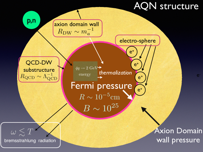
Figure 1: AQN-structure (not in scale), adopted from [32]. The dominant portion of the energy $\sim 2$ GeV produced as a result of a single annihilation process inside the anti-nugget is released in form of the bremsstrahlung radiation with frequencies $\omega\leq T$, see description and notations in the main text.

When the AQN enters the region of the baryon density $n$ the annihilation processes start and the internal temperature increases. A typical internal temperature $T$ of the AQNs for very dilute galactic environment can be estimated from the condition that the radiative output must balance the flux of energy onto the nugget

$$F_{\rm{tot}}(T)(4\pi R^{2})\approx\kappa\cdot(\pi R^{2})\cdot(2~{}{\rm GeV})\cdot n\cdot v_{\rm AQN},$$ (2)

where $n$ represents the baryon number density of the surrounding material, and $F_{\rm{tot}}(T)$ is total surface emissivity, see below. The left hand side accounts for the total energy radiation from the AQN’s surface per unit time while the right hand side accounts for the rate of annihilation events when each successful annihilation event of a single baryon charge produces $\sim 2m_{p}c^{2}\approx 2~{}{\rm GeV}$ energy. In Eq. (2) we assume that the nugget is characterized by the geometrical cross section $\pi R^{2}$ when it propagates in environment with local baryon density $n$ with velocity $v_{\rm AQN}\sim 10^{-3}c$. The factor $\kappa$ accounts for large theoretical uncertainties related to the annihilation processes of the (antimatter) AQN colliding with surrounding material.

The total surface emissivity due to the bremsstrahlung radiation from electrosphere at temperature $T$ has been computed in [31] and it is given by

$$F_{\rm{tot}}\approx\frac{16}{3}\frac{T^{4}\alpha^{5/2}}{\pi}\sqrt[4]{\frac{T}{m}}\,,$$ (3)

where $\alpha\approx 1/137$ is the fine structure constant, $m=511{\rm\,keV}$ is the mass of electron, and $T$ is the internal temperature of the AQN. One should emphasize that the emission from the electrosphere is not thermal, and the spectrum is dramatically different from blackbody radiation. From (2) one can estimate a typical internal nugget’s temperature when density $n$ assumes the typical values $n\sim\rm cm^{-3}$ relevant for this work:

$$T\sim 0.4~{}{\rm eV}\cdot\left(\frac{n}{\rm cm^{-3}}\right)^{\frac{4}{17}}\cdot\left(\frac{v_{\rm AQN}}{10^{-3}c}\right)^{\frac{4}{17}}\cdot\kappa^{\frac{4}{17}}.$$ (4)

It strongly depends on unknown parameter $\kappa$ as mentioned above. In case which is relevant for our studies when the surrounding material is a highly ionized plasma the parameter $\kappa$ effectively gets much larger as the AQN (being negatively charged, see below) attracts more positively charged ions from surrounding material. This attraction consequently effectively increases the cross section and the rate of annihilation, eventually resulting in a larger value of $T$.

Another feature which is relevant for our present studies is the ionization properties of the AQN. Ionization, as usual, occurs in a system as a result of the high internal temperature $T$. In our case of the AQN characterized by temperature (4) a large number of weakly bound positrons $\sim Q$ from the electrosphere get excited and can easily leave the system. The corresponding parameter $Q$ can be estimated as follows:

$$Q\approx 4\pi R^{2}\int^{\infty}_{0}n(z,T)\mathrm{d}z\sim\frac{4\pi R^{2}}{\sqrt{2\pi\alpha}}\left(mT\right)\left(\frac{T}{m}\right)^{\frac{1}{4}},~{}~{}$$ (5)

where $n(z,T)$ is the local density of positrons at distance $z$ from the nugget’s surface, which has been computed in the mean field approximation in [31] and has the following form

$$n(z,T)=\frac{T}{2\pi\alpha}\frac{1}{(z+\bar{z})^{2}},~{}~{}~{}~{}\bar{z}^{-1}\approx\sqrt{2\pi\alpha}\cdot m\cdot\left(\frac{T}{m}\right)^{\frac{1}{4}},~{}~{}~{}~{}$$ (6)

where $\bar{z}$ is the integration constant is chosen to match the Boltzmann regime at sufficiently large $z\gg\bar{z}$. Numerical studies   [33] support the approximate analytical expression (6).

Numerically, the number of weakly bound positrons can be estimated from (5) as follows:

$$Q\approx 1.5\cdot 10^{6}\left(\frac{T}{\rm eV}\right)^{\frac{5}{4}}\left(\frac{R}{2.25\cdot 10^{-5}\rm cm}\right)^{2}.$$ (7)

In what follows we assume that, to first order, that the finite portion of positrons $\sim Q$ leave the system as a result of the complicated processes mentioned above, in which case the AQN as a system acquires a negative electric charge $\sim-|e|Q$ and get partially ionized as a macroscopically large object of mass $M\simeq m_{p}B$. The ratio $eQ/M\sim 10^{-19}e/m_{p}$ characterizing this object is very tiny. However, the charge $Q$ itself is sufficiently large being capable to capture (with consequent possibility of annihilation) the positively charged protons from surrounding ionized plasma.

The corresponding capture radius $R_{\rm cap}(T)$ can be estimated from the condition that the potential energy of the attraction (being negative) is the same order of magnitude as kinetic energy of the protons from highly ionized gas with $x_{e}=1$ which is characterized by external temperature $T_{\rm gas}$, i.e.

$$\frac{\alpha Q(T)}{R_{\rm cap}(T)}\sim\frac{m_{p}v^{2}}{2}\sim T_{\rm gas}~{}~{}\Rightarrow~{}~{}~{}R_{\rm cap}(T)\simeq 0.2~{}{\rm cm}\left(\frac{T}{\rm eV}\right)^{\frac{5}{4}}\cdot\left(\frac{\rm eV}{T_{\rm gas}}\right),$$ (8)

where $Q$ is estimated by (5), (7). One should emphasize that $R_{\rm cap}(T)$ depends on both temperatures, the internal $T$ through the charge $Q(T)$ as given by (5), (7) and external gas temperature $T_{\rm gas}$ which is essentially determined by the typical velocities of particles in plasma and can be identified with virial temperature of particles in galaxy. Important point here is that $R_{\rm cap}(T)\gg R$ such that effective cross section being $\pi R_{\rm cap}^{2}$ is dramatically larger than geometric size $\pi R^{2}$ entering (2) which would be the case if gas is represented by neutral atoms. In our relation (8) we also neglected the Debye screening effect as $\lambda_{D}\gg R_{\rm cap}$ for all relevant values of parameters, where $\lambda_{D}$ is defined as usual

$$\lambda_{D}\approx\sqrt{\frac{T_{\rm gas}}{4\pi\alpha n}}\sim 0.7\cdot 10^{3}~{}{\rm cm}\left({\frac{T_{\rm gas}}{\rm eV}}\right)^{1/2}.$$ (9)

Precisely this feature of ionization of the AQN characterized by electric charge $Q(T)$ dramatically enhances the visible-DM interaction in highly ionized environment when cosmologically relevant ratio ($\sigma/M)$ from table 1 becomes large. We illustrate this enhancement with the following estimates of this ratio for the neutral ($x_{e}=0$) and highly ionized ($x_{e}=1$) environments:

$$\frac{\sigma(x_{e}=0)}{M_{N}}\sim\frac{\pi R^{2}}{M_{N}}\sim 10^{-10}{\rm\frac{cm^{2}}{g}},~{}~{}~{}~{}~{}~{}~{}~{}~{}~{}~{}~{}\frac{\sigma(x_{e}=1)}{M_{N}}\sim\frac{\pi R_{\rm cap}^{2}}{M_{N}}\sim{\rm\frac{cm^{2}}{g}}\left(\frac{T}{10~{}\rm eV}\right)^{\frac{5}{2}}\cdot\left(\frac{\rm eV}{T_{\rm gas}}\right)^{2}.$$ (10)

We conclude this brief overview section on previous works on the AQNs with the following remark: all the parameters of the model as reviewed above had been applied previously for dramatically different studies, in very different circumstances as highlighted in concluding section 5. We do not modify any fundamental parameters of this model by applying this new DM scenario in next section 3 to the problem on structure formation. In particular we shall argue that some puzzling observations such as (1) could be a direct consequence of such visible- DM interaction (10), when the AQNs indeed behave as chameleon like particles. To be more precise, the effective cross section (10) is highly sensitive to the density of the surrounding environment $n$, its temperature $T_{\rm gas}$ and its ionization features $x_{e}$. The corresponding parameters affect the strength of visible-DM interaction and its key element, $R_{\rm cap}(T)$, which itself depends on the environment according to (4) and (8).

3 DM-visible matter coupling

Our basic claim of this section is that the structure formation may be dramatically affected by the DM in form of the AQNs which strongly interact with the gas of particles. The study of the structure formation dynamics is obviously a prerogative of the numerical simulations, which is the main technical tool for quantitive analysis. The goal of this work is less ambitious as we want to demonstrate in a pure qualitative analytical way few important characteristics (such as portion of the ionization of the gas, $x_{e}$) which may be dramatically affected by the interaction of the AQNs with surrounding plasma during the structure formation.

To demonstrate the importance of these key novel qualitative effects is very instructive to compare the analytical formula of our studies with corresponding conventional expressions which are normally used in numerical simulations. Therefore, in what follows we use analytical formulae from the textbook [34] as the benchmark to be compared with corresponding AQN-based expressions. We shall demonstrate that the DM-visible matter coupling will play the dominant role in some circumstances. The corresponding effects may dramatically modify the conventional picture of the structure formation. Our analytical studies obviously do not replace a full scale numerical simulations. However, the comparison with conventional formulae [34] obviously show the basic trend which may crucially modify some elements of the standard picture on structure formation. These modifications have in fact, many common consequences and manifestations with previously introduced ad hoc models which were coined as Self-Interacting dark matter, Self-Annihilating dark matter, Decaying dark matter etc.

Our comment here is that the AQN model was invented (in contrast to all ad hoc models mentioned above) for dramatically different purposes as overviewed in Sect. 2.1 with drastically different motivation, not related in anyway to the structure formation problems being the main topic of this work. Nevertheless, there are many model-independent consequences of the AQN construction which may dramatically affect the dynamics at small scales as we argue below in section 3.2.

3.1 Galaxy Formation. The basics picture. Notations.

The conventional picture of the structure formation assumes that CCDM particles have undergone violent relaxation such that the asymptotic density distribution $\rho_{\rm DM}(r)$ can be approximated by an isothermal sphere [34]. If effects of baryon’s cooling are ignored the dynamical evolution of the baryons will be similar to that of DM particles. However, the collapse of baryons develops shocks and the gas get reheated to a temperature $T_{\rm gas}$ at which the pressure balance can prevent further collapse. The corresponding temperature can be estimated as follows [34]:

$$\frac{3\rho_{\rm gas}T_{\rm gas}}{2m_{p}}\simeq\frac{\rho_{\rm gas}v^{2}}{2}~{}~{}~{}~{}~{}\Rightarrow~{}~{}~{}~{}~{}T_{\rm gas}\simeq\frac{m_{p}v^{2}}{3},~{}~{}~{}{\rm where}~{}~{}~{}\frac{v^{2}}{r}\simeq\frac{GM(r)}{r^{2}},$$ (11)

where for an order of magnitude estimates and for simplification we assumed that the gas is entirely consist the hydrogen, though the He fraction could be relatively large. The velocity $v$ entering (11) is the circular velocity not to be confused with mean-square velocity $\sigma_{v}^{2}=1/2v^{2}$. The $T_{\rm gas}$ as defined by (11) is essentially the virial temperature $T_{\rm vir}$, but we prefer to use notation $T_{\rm gas}$ as our goal is to study the microscopical interaction of this gas with the AQNs in what follows.

As the temperature $T_{\rm gas}$ becomes sufficiently high the cooling processes must be taken into account. If the cooling processes are sufficiently effective the collapse may proceed further to form more tightly bound object. The corresponding evolution is entirely determined by the relative values of the dynamical time scale $t_{\rm dyn}$ and the cooling time scale $t_{\rm cool}$ defined as follows [34]:

$$t_{\rm dyn}\simeq\frac{\pi}{2}\left(\frac{R^{3}}{2GM}\right)^{\frac{1}{2}}\simeq 5\cdot 10^{7}{\rm yr}\left(\frac{\rm GeV\cdot cm^{-3}}{\rho_{\rm total}}\right)^{\frac{1}{2}},~{}~{}~{}t_{\rm cool}\equiv\frac{E}{\dot{E}}\simeq\frac{3}{2}\frac{n_{\rm gas}T_{\rm gas}}{\Lambda(T_{\rm gas})},~{}~{}~{}\rho_{\rm total}\equiv(\rho_{\rm gas}+\rho_{\rm DM})$$ (12)

where $n_{\rm gas}$ is the number density of the material such that $\rho_{\rm gas}\equiv m_{p}n_{\rm gas}$, while $\Lambda(T_{\rm gas})$ is the cooling rate which has the meaning of energy emitted from unit volume per unit time with dimensionality $\rm[erg\cdot cm^{-3}\cdot s^{-1}]$. In all these estimates, including (12) we simplify things and ignore the He portion of the gas as we already mentioned above.

The cooling rate is dominated by two processes: the energy loss due to the bremsstrahlung [34]

$$\epsilon_{\rm brem}\simeq 1.4\cdot 10^{-27}{\rm\frac{erg}{cm^{3}\cdot s}}\left(\frac{T_{\rm gas}}{1K}\right)^{1/2}\left(\frac{n_{\rm gas}}{\rm cm^{-3}}\right)^{2}x_{e}^{2},$$ (13)

and the loss due to the atomic collisions [34]

$$\epsilon_{\rm coll}\simeq 7.5\cdot 10^{-19}{\rm\frac{erg}{cm^{3}\cdot s}}\left(\frac{n_{\rm gas}}{\rm cm^{-3}}\right)^{2}x_{e}(1-x_{e})\exp\left(-\frac{E_{0}}{T_{\rm gas}}\right),$$ (14)

where $x_{e}$ is the ionization fraction and $E_{0}=13.6~{}\rm eV$. Both rates $\epsilon_{\rm brem}$ and $\epsilon_{\rm coll}$ dramatically depend on ionization portion of the gas, the $x_{e}(T_{\rm gas})$ which itself is function of the gas temperature $T_{\rm gas}$.

The corresponding parameter $x_{e}(T_{\rm gas})$ is determined by the relative strength of two competing processes: the collisional ionization which is characterized by the time scale $t_{i}$ and the recombination with time scale $t_{r}$. The corresponding time scales can be estimated as follows [34]:

$$t_{i} \simeq \frac{2.2\cdot 10^{14}{\rm s}}{(1-x_{e})}\left(\frac{10^{5}K}{T_{\rm gas}}\right)^{1/2}\exp\left(\frac{E_{0}}{T_{\rm gas}}\right),$$ (15)

$$t_{r} \simeq \frac{5.8\cdot 10^{19}{\rm s}}{(x_{e})}\left(\frac{T_{\rm gas}}{10^{5}K}\right)^{2/3}.$$ (16)

Equating (15) and (16) determines the ionization fraction $x_{e}(T_{\rm gas})$ as a function of $T_{\rm gas}$,

$$x_{e}(T_{\rm gas})\simeq\left[1+2.8\cdot 10^{-6}\left(\frac{10^{5}K}{T_{\rm gas}}\right)^{7/6}\exp\left(\frac{E_{0}}{T_{\rm gas}}\right)\right]^{-1}.$$ (17)

This expression for $x_{e}(T_{\rm gas})$ can be substituted to formulae for $\epsilon_{\rm brem}$ and $\epsilon_{\rm coll}$ as given by (13) and (14) correspondingly to estimate the key parameter, the cooling rate $\Lambda(T_{\rm gas})$ entering formula (12). Assuming that $x_{e}(T_{\rm gas})\simeq 1$ one can expand (17) to arrive to the following simplified expression for the cooling rate which is not valid for low temperatures when $x_{e}$ strongly deviates from unity and expansion is not justified,

$$\Lambda(T_{\rm gas})\simeq 10^{-24}{\rm\frac{erg}{cm^{3}\cdot s}}\left[0.44\left(\frac{T_{\rm gas}}{10^{5}K}\right)^{1/2}+2.1\left(\frac{T_{\rm gas}}{10^{5}K}\right)^{-7/6}\right],~{}~{}~{}(\epsilon_{\rm coll}+\epsilon_{\rm brem})\equiv\left(\frac{n_{\rm gas}}{\rm cm^{-3}}\right)^{2}\Lambda(T_{\rm gas}).$$ (18)

In this formula the first term in the brackets is due to bremsstrahlung radiation $\epsilon_{\rm brem}$ while the second term is the result of atomic collisions $\epsilon_{\rm coll}$.

The cooling time scale $t_{\rm cool}$ can be estimated from (12) as follows

$$t_{\rm cool}\equiv\frac{E}{\dot{E}}\simeq 2.5\cdot 10^{6}{\rm yr}\left(\frac{\rm cm^{-3}}{n_{\rm gas}}\right)\left[\left(\frac{T_{\rm gas}}{10^{5}K}\right)^{-1/2}+4.8\left(\frac{T_{\rm gas}}{10^{5}K}\right)^{-13/6}\right]^{-1},$$ (19)

where we literally use expression for $\Lambda(T_{\rm gas})$ as given by (18). The numerical value in the brackets for the second term (which describes the cooling due to the atomic collisions $\epsilon_{\rm coll}$) slightly deviates from the corresponding formula from the textbook [34]. This is because the expression in [34] was modified to better fit with the numerical simulation results. We opted to keep the original expressions (18) as our main goal is the comparison of the AQN-induced mechanism with conventional mechanism to pinpoint the dramatic qualitative deviations from the standard cooling processes as given by (19).

The estimate for the cooling time scale $t_{\rm cool}$ allows us to compare it with the dynamical time scale $t_{\rm dyn}$ as given by (12), where matter density should be understood as the total matter density of the material, including the DM portion. It is convenient to define the ratio $\cal R$ as follows:

$${\cal R}\equiv\frac{t_{\rm cool}(\rho_{\rm gas})}{t_{\rm dyn}(\rho_{\rm total})}\leq 1,~{}~{}~{}~{}~{}~{}\rho_{\rm total}\equiv(\rho_{\rm gas}+\rho_{\rm DM}),$$ (20)

when $t_{\rm cool}(\rho_{\rm gas})$ depends exclusively from hadronic gas component $\rho_{\rm gas}$ in CCDM treatment, while $t_{\rm dyn}(\rho_{\rm total})$ depends on the total density of the material, including the DM component.

If $\cal R$ is smaller than unity the cloud will cool rapidly, and gas will undergo (almost) a free fall collapse. Fragmentation into smaller units occurs because smaller mass scales will become gravitationally unstable. The key parameter which determines the parametrical space when the clouds will continue to collapse defines the region when the galaxies (and stars) may form. Precisely this parameter $\cal R$ governs the evolution of the system. One can estimate the typical masses, typical sizes, and the typical temperatures $T_{\rm gas}$ of the clouds for this collapse to happen based on analysis of domain where ${\cal R}\leq 1$. The corresponding studies are obviously a prerogative of the numerical N-body simulations, far outside of the scope of the present work, though some qualitative estimates can be also made [34].

For the purposes of the present work we use the condition (20) as the boundary in parametrical space which specifies the domain when the galaxies may form. We will specifically pinpoint some key modifications of this parameter ${\cal R}$ when the AQNs are present in the system and dramatically modify this domain. Our crucial observation is that $t_{\rm cool}$ will depend on both: the visible $\rho_{\rm gas}$ and dark matter $\rho_{\rm DM}$ components, which qualitatively modifies condition (20). The corresponding analysis represents the topic of the next section 3.2.

One should note that all parameters and formulae we use in this section as benchmarks are taken from the textbook [34]. They are obviously outdated in comparison with the standard parameters being used in more recent papers. Nevertheless, we opted to use the parameters and numerics literally from [34] to pinpoint the key differences (in comparison with the conventional treatment of the problem) which occur when the AQN-induced interaction is taken into account. It is very instructive to understand a precise way how the new physics enters and modifies the standard picture in a qualitative parametrical way.

3.2 Galaxy Formation. The AQN-induced modifications.

As we discussed in previous section the cooling rate is very sensitive to the ionization fraction $x_{e}(T_{\rm gas})$ as given by (13) and (14). In conventional picture this factor $x_{e}(T_{\rm gas})$ is determined by two competing processes as represented by expression (17). The main goal of this section is to demonstrate that this estimate for $x_{e}(T_{\rm gas})$ is dramatically modified in the presence of the AQNs. As a result the expression for the cooling rate $t_{\rm cool}$ as given by (19) is also changed. These changes lead to drastic modification of the domain governed by parameter ${\cal R}\leq 1$ when the structure formation can be formed. One of the main qualitative consequences of these modifications is emergence of the relations such as (1) reflecting a strong visible-DM coupling, which was one of the motivations for the present studies.

The main physics process which leads to such dramatic variations can be explained as follows. The AQNs start to interact with surrounding material, mostly protons when the density of the gas becomes sufficiently high, around $(1~{}\rm cm^{-3})$. The corresponding interaction is strongly enhanced in the ionized plasma due to the long-ranged Coulomb attraction between (negatively charged) AQNs and protons. This enhancement of the visible- DM interaction may dramatically decrease the ionization fraction $x_{e}$ of plasma due to the capturing (with consequent annihilation) of the protons from plasma and subsequent emission of positrons from AQN’s electrosphere. These positrons will eventually annihilate with free electrons from the plasma. The corresponding time scale $t_{\rm AQN}$ for this process could be dramatically smaller than the recombination time scale $t_{r}$ estimated by (16). As a result the AQN-proton annihilation becomes the dominant processes which dramatically reduces the ionization fraction $x_{e}$ of plasma. As explained above the ionization fraction directly affects the domain of the parametrical space where ${\cal R}\leq 1$ which describes the region where the galaxies may form.

Now we proceed with corresponding estimates. First, we estimate the number of protons being captured by AQNs per unit volume per unit time,

$$\frac{dn}{dtdV}\approx\pi R^{2}_{\rm cap}(T)\cdot n_{p}\cdot n_{\rm AQN}\cdot v_{\rm AQN},$$ (21)

where $R_{\rm cap}(T)$ is the capture radius determined by condition (8) when the protons from the surrounding plasma are captured by the negatively charged AQNs and will be eventually annihilated inside the nugget’s core. The formula (21) explicitly shows the key role of the ionized media as the cross section for annihilation of the neutral atoms is dramatically smaller as $R\ll R_{\rm cap}(T)$. By dividing expression (21) by gas number density $n$ we arrive to estimation for the frequency of the capturing (with consequent annihilation) of the protons. It is more convenient to represent this as time scale $t_{\rm AQN}$ for capturing of a proton from plasma by AQNs:

$$t_{\rm AQN}\approx\left[\pi R^{2}_{\rm cap}(T)\cdot n_{\rm AQN}\cdot v_{\rm AQN}\cdot x_{e}\right]^{-1},~{}~{}~{}n_{p}\equiv x_{e}n_{\rm gas},~{}~{}~{}n_{\rm AQN}(r)\approx\frac{\rho_{\rm DM}(r)}{m_{p}\langle B\rangle},$$ (22)

where $v_{\rm AQN}\approx v$ is the same order of magnitude as the circular velocity as both are determined by pure gravitational forces (11). The time scale $t_{\rm AQN}$ plays the key role in our discussions which follow because it competes with the recombination time scale (16) when both processes decrease the ionization fraction $x_{e}$.

Numerically the time scale $t_{\rm AQN}$ can be estimated as follows:

$$t_{\rm AQN}\approx\frac{0.5\cdot 10^{19}{\rm s}}{(x_{e})}\left(\frac{T_{\rm gas}}{10^{5}K}\right)^{3/2}\cdot\left(\frac{T}{10^{5}K}\right)^{-5/2}\cdot\left(\frac{\rho_{\rm DM}(r)}{\rm GeV\cdot cm^{-3}}\right)^{-1},$$ (23)

which is almost one order of magnitude faster than the recombination time scale $t_{r}$ as estimated by (16) for typical parameters ${T_{\rm gas}}\sim{10^{5}K}$. One should comment here that the external temperature of the plasma ${T_{\rm gas}}$ and internal temperature $T$ of the AQN’s electrosphere are different parameters of the system, though in the galactic environment they may assume similar numerical values. One should also note here that the recombination process and the capturing of the proton by AQNs with its consequent annihilation inside the nugget work in the same direction by decreasing the ionization fraction $x_{e}$.

To estimate the ionization fraction $x_{e}(T_{\rm gas})$ when the AQN annihilation processes are operational one should equalize

$$t_{i}^{-1}=t_{r}^{-1}+t_{\rm AQN}^{-1}$$ (24)

which replaces the condition $t_{i}=t_{r}$ leading to previous expression (17) for $x_{e}(T_{\rm gas})$. To simplify the problem we consider the region when $t_{\rm AQN}\ll t_{r}$ and the recombination process can be ignored. The corresponding condition is:

$$t_{\rm AQN}\ll t_{r}~{}~{}~{}\Rightarrow~{}~{}~{}\left(\frac{\rho_{\rm DM}(r)}{\rm GeV\cdot cm^{-3}}\right)\cdot\left(\frac{T_{\rm gas}}{10^{5}K}\right)^{-\frac{5}{6}}\cdot\left(\frac{T}{10^{5}K}\right)^{\frac{5}{2}}\gg 0.1,$$ (25)

which implies that for sufficiently high DM density $\rho_{\rm DM}\sim 5m_{p}n(r)$ with $n(r)\sim{\rm cm^{-3}}$ or/and sufficiently low gas temperature $T_{\rm gas}\leq{10^{6}K}$ the AQN-induced processes dominate, in which case the ionization fraction $x_{e}(T_{\rm gas})$ is entirely determined by the competition of the collisional ionization time scale $t_{i}$ and $t_{\rm AQN}$.

Equating $t_{\rm AQN}$ and $t_{i}$ we arrive to the following estimate for $x_{e}(T_{\rm gas})$:

$$x_{e}(T_{\rm gas})\simeq\left[1+4.4\cdot 10^{-5}\left(\frac{10^{5}K}{T_{\rm gas}}\right)^{2}\cdot\left(\frac{T}{10^{5}K}\right)^{\frac{5}{2}}\cdot\left(\frac{\rho_{\rm DM}(r)}{\rm GeV\cdot cm^{-3}}\right)\cdot\exp\left(\frac{E_{0}}{T_{\rm gas}}\right)\right]^{-1}~{}~{}{\rm(AQN-induced).}$$ (26)

This expression replaces the previous formula for $x_{e}(T_{\rm gas})$ in conventional scenario (17). Assuming that the condition (25) is satisfied and $x_{e}(T_{\rm gas})\approx 1$ one can expand (26) to arrive to the following expression for $(1-x_{e})$ entering the cooling rate due to the atomic collisions (14):

$$[1-x_{e}(T_{\rm gas})]\simeq 4.4\cdot 10^{-5}\left(\frac{10^{5}K}{T_{\rm gas}}\right)^{2}\cdot\left(\frac{T}{10^{5}K}\right)^{\frac{5}{2}}\cdot\left(\frac{\rho_{\rm DM}(r)}{\rm GeV\cdot cm^{-3}}\right)\cdot\exp\left(\frac{E_{0}}{T_{\rm gas}}\right).$$ (27)

Now we can substitute this expression for $(1-x_{e})$ to the formula (14) for the cooling rate due to the atomic collisions:

$$\epsilon_{\rm coll}\simeq 3.4\cdot 10^{-23}{\rm\frac{erg}{cm^{3}\cdot s}}\left(\frac{n_{\rm gas}}{\rm cm^{-3}}\right)^{2}\cdot\left(\frac{T_{\rm gas}}{10^{5}K}\right)^{-2}\cdot\left(\frac{T}{10^{5}K}\right)^{\frac{5}{2}}\cdot\left(\frac{\rho_{\rm DM}(r)}{\rm GeV\cdot cm^{-3}}\right)~{}~{}{\rm(AQN-induced).}$$ (28)

At the same time the expression for cooling due to the bremsstrahlung radiation $\epsilon_{\rm brem}$ remains the same as it is not sensitive to $x_{e}$ as long as it is close to unity. As a result, the expression for the cooling rate $\Lambda(T_{\rm gas})$ assumes the form

$$\Lambda(T_{\rm gas})\simeq 10^{-24}{\rm\frac{erg}{cm^{3}\cdot s}}\left[0.44\left(\frac{T_{\rm gas}}{10^{5}K}\right)^{\frac{1}{2}}+34\left(\frac{T_{\rm gas}}{10^{5}K}\right)^{-2}\left(\frac{T}{10^{5}K}\right)^{\frac{5}{2}}\left(\frac{\rho_{\rm DM}(r)}{\rm GeVcm^{-3}}\right)\right],$$ (29)

where the first term due to the bremsstrahlung radiation remains the same as in the conventional treatment (18), while the second term describing the atomic collisions is dramatically larger by one order of magnitude than in (18). The basic reason for this difference is that the cooling rate due to the atomic collisions is proportional to density of the neutral atoms $n_{H}\propto(1-x_{e})$ which increases in the presence of the AQNs in comparison with conventional case due to the mechanism described at the very beginning of this section.

The increase of the cooling rate $\Lambda(T_{\rm gas})$ leads to consequent dramatic modification in the cooling time scale $t_{\rm cool}$ as defined by (19). In the presence of the AQNs in the system it gets modified as follows:

$$t_{\rm cool}\equiv\frac{E}{\dot{E}}\simeq 2.5\cdot 10^{6}{\rm yr}\left(\frac{\rm cm^{-3}}{n_{\rm gas}}\right)\left[\left(\frac{T_{\rm gas}}{10^{5}K}\right)^{-1/2}+77\left(\frac{T_{\rm gas}}{10^{5}K}\right)^{-3}\left(\frac{T}{10^{5}K}\right)^{\frac{5}{2}}\left(\frac{\rho_{\rm DM}(r)}{\rm GeV\cdot cm^{-3}}\right)\right]^{-1},$$ (30)

where the first term in the brackets due to the bremsstrahlung radiation remains the same as in the conventional treatment (19), while the second term describing the atomic collisions is dramatically enhanced in comparison with (19) due to the same reasons described above.

There are two key points here: first, $t_{\rm cool}$ depends on $\rho_{\rm DM}(r)$ which is a highly nontrivial new qualitative effect because in conventional CCDM picture any cooling effects fundamentally cannot depend on $\rho_{\rm DM}(r)$ as these effects are entirely determined by the visible baryonic matter in form of the gas. The second point here is that for the temperatures $T_{\rm gas}\leq 10^{5}K$ the cooling time scale $t_{\rm cool}$ is one order of magnitude shorter than in conventional treatment (19). In fact, the AQN-induced processes remain to be the dominant cooling mechanism up to $T_{\rm gas}\simeq 10^{6}K$ for $\rho_{\rm DM}\approx 5\rho_{\rm gas}$, and could remain the dominant mechanism even for higher temperatures.

The dramatic modifications in $t_{\rm cool}$ implies that the key parameter ${\cal R}$ will also experience crucial qualitative changes in defining of the domain where the structure formation may form,

$${\cal R}\equiv\frac{t_{\rm cool}(\rho_{\rm gas},\rho_{DM})}{t_{\rm dyn}(\rho_{\rm total})}\leq 1,~{}~{}~{}~{}~{}~{}\rho_{\rm total}\equiv(\rho_{\rm gas}+\rho_{\rm DM}).$$ (31)

Indeed, in contrast with the original definition (20) the cooling time $t_{\rm cool}(\rho_{\rm gas},\rho_{DM})$ entering (31) now depends explicitly on both, the $\rho_{\rm gas}$ and $\rho_{DM}$ as expression (30) explicitly shows.

We conclude this section with the following generic comment. We have made a large number of technical assumptions in this section to simplify the analysis to argue that the visible-DM interaction may dramatically modify some parameters, such as $x_{e}$ and cooling time $t_{\rm cool}$ as a result of the AQN-induced processes. It was not the goal of this work to perform a full scale simulations and modelling, which is well beyond the scope of the present work. However, we observed a number of qualitative features of the system, which are known to occur, but cannot be easily understood within conventional models of structure formation. In next section 4 we briefly overview some observational consequences of the AQN framework, which are hard to understand within conventional models, but could be easily understood within a new paradigm when the baryonic and DM constituents become strongly interacting components of the system.

4 Observable consequences of the visible-DM interaction. The New Paradigm.

As we reviewed in Sect.2 the AQN model is dramatically distinct from conventional DM proposals as the central elements of the DM configurations are the same (anti)quarks and gluons from QCD which represents the inherent part of the Standard Model (SM). Therefore, the AQNs become the strongly interacting objects in sufficiently dense environment. In other words, the AQN behaves as a chameleon: it does not interact with the surrounding material in dilute neutral environment, but it becomes strongly interacting object in sufficiently dense environment. Therefore, the AQN framework essentially represents an explicit realization of the New Paradigm, when the visible and DM building blocks become strongly interacting components if some conditions are met. It must be contrasted with conventional CCDM paradigm when these distinct components, by definition, never couple.

The main purpose of this section is to briefly overview a number of qualitative consequences of this new paradigm. The corresponding properties which are listed below are not very sensitive to any specific numerical values of the parameters used in the previous sections. Instead, these novel features represent the inherent features of the new framework. In next subsection 4.1 we explain in qualitative way how the observed correlation such as (1) could emerge in the New Paradigm. In section 4.2 we argue that the new paradigm inevitably implies emission of the additional energy in different frequency bands, including the UV radiation. Apparently, there are several recent hints from JWST, see e.g. [10, 11, 12, 13] that such excess of radiation has been indeed observed at large $z$. In section 4.3 we argue that the very same effects could be responsible for the mysterious diffuse UV radiation [14, 15, 16] at present time $z=0$ as suggested in [17].

4.1 How the observed correlation (1) could emerge in the New Paradigm?

To simplify our qualitative analysis we consider the domain in the parametrical space when the AQN-induced term dominates the conventional cooling due to the bremsstrahlung radiation. The corresponding condition can be estimated from (30) as follows:

$$\left(\frac{T_{\rm gas}}{10^{6}K}\right)^{-\frac{5}{2}}\left(\frac{T}{10^{5}K}\right)^{\frac{5}{2}}\left(\frac{\rho_{\rm DM}(r)}{\rm GeV\cdot cm^{-3}}\right)\gg 4.1,$$ (32)

which is satisfied in the region with $T_{\rm gas}\leq{10^{6}K}$ and $\rho_{\rm DM}\geq 5\rho_{\rm gas}$ with our benchmark density $n_{\rm gas}\approx\rm cm^{-3}$. This parametrical region is largely overlap with condition (25) that the AQN-induced processes dominate conventional recombination effects in computations of the ionization fraction $x_{e}$ such that all our simplification and estimates remain consistent.

Therefore, assuming the condition (32) is satisfied our basic requirement (31) defining the domain ${\cal R}\leq 1$ where galaxy may form can be written in the following simple way

$$\frac{[\tilde{\rho}_{\rm DM}\cdot\tilde{\rho}_{\rm gas}]}{\sqrt{\tilde{\rho}_{\rm DM}+\tilde{\rho}_{\rm gas}}}\left(\frac{T_{\rm gas}}{10^{6}K}\right)^{-3}\left(\frac{T}{10^{5}K}\right)^{\frac{5}{2}}\geq 6.5,~{}~{}~{}~{}\tilde{\rho}_{\rm DM}\equiv\left(\frac{\rho_{\rm DM}(r)}{\rm GeV\cdot cm^{-3}}\right),~{}~{}~{}~{}\tilde{\rho}_{\rm gas}\equiv\left(\frac{\rho_{\rm gas}(r)}{\rm GeV\cdot cm^{-3}}\right),$$ (33)

where we use formula (12) for the $t_{\rm dyn}$ and expression (30) for $t_{\rm cool}$ assuming the AQN-induced term dominates according to the condition (32).

The crucial point here is that the visible-DM interaction representing the key element of a new paradigm explicitly manifests itself in formula (33) which strongly resembles the structure of the correlation (1) inferred from the observations long ago, see review [5]. The coupling of the visible and dark components is explicitly present in the system, and formula (33) is a direct consequence of this interaction.

It is important to emphasize that the condition (33) is local in nature as it depends on $[\tilde{\rho}_{\rm DM}(r)\cdot\tilde{\rho}_{\rm gas}(r)]$ in region $r\leq r_{0}$ where the densities are sufficiently large, roughly $\rho_{\rm DM}(r)\sim\rho_{\rm gas}(r)\sim 10^{-24}{\rm(g\cdot cm^{-3}})$ in cgs units. For $r\gg r_{0}$ the the visible-DM interaction can be ignored and the AQNs behave in all respects as CCDM. The locality of the condition (33) implies that region $r_{0}$ where the visible-DM interaction becomes the dominant element of the system does not depend on the size of the cloud which is about to collapse to form a galaxy, nor on its mass, which is precisely the claim of [5] as stated in (1).

Parameter $r_{0}$ was identified with the size of the core in [5], while in our microscopical treatment of the system the scale $r_{0}$ is identified with condition (33). Therefore, the core formation in the AQN framework can be interpreted as a result of strong visible- DM interaction when condition (33) starts to satisfy at $r\approx r_{0}$.

The temperature $T_{\rm gas}$ entering (33) can be thought as the virial temperature as defined by (11), which indeed assume the values in the range $T_{\rm gas}\simeq(10^{5}-10^{6})K$. Another parameter $T$ entering (33) is the internal temperature of the AQNs, and should not be confused with $T_{\rm gas}$. This parameter is very hard to estimate as reviewed in section 2, but it must also lie in the range $T\simeq(10^{5}-10^{6})K$ for the environment under consideration. We shall not elaborate in details on this matter in the present work.

4.2 The AQNs as the UV emitters in early galaxies

The processes which lead to the correlation (33) as discussed above are always accompanied by the radiation in many different frequency bands as we discuss below. Indeed, the total amount of energy being produced per unit time is determined by the right hand side of (2). This energy will be released into the space in many different forms, including the axion and neutrino emissions. However, the dominant portion of the emission will be in form of radiation from electrosphere according to (3). The spectrum of the radiation is very broad $\omega\leq T$ as computed in [31] and depicted on Fig. 1. This is the dominant radiation process. There is also annihilation of the emitted positrons with electrons from plasma as mentioned in footnote 3. However, the total released energy due to these annihilation processes is obviously suppressed by factor $m_{e}/m_{p}\ll 1$. In what follows we estimate the total amount of energy being produced as a result of the annihilation processes during the galaxy formation.

We start from expression (21) for number of annihilation events per unit time per unit volume. We multiply this expression by factor $2m_{p}c^{2}\simeq 2\rm~{}GeV$ to arrive to estimate for energy being produced as a result of these annihilation processes:

$$\frac{dE}{dtdV}\approx\pi R^{2}_{\rm cap}(T)\cdot n\cdot n_{\rm AQN}\cdot v_{\rm AQN}\cdot x_{e}\cdot(\rm 2~{}GeV)$$ (34)

By dividing expression (34) by gas number density $n$ we arrive to estimation of the energy being released per unit time per single proton (or hydrogen atom) in plasma. To estimate the total energy being released by this mechanism we have to multiply the estimate (34) by the Hubble time at redshift $z$. Thus, we arrive to an order of magnitude estimate for the total energy released by the AQNs due to the annihilation events during the Hubble time per single proton (or hydrogen atom) in plasma:

$$\frac{dE}{dt}H^{-1}\sim{4\cdot 10^{-7}}~{}{\rm GeV}\cdot x_{e}\cdot\left(\frac{T_{\rm gas}}{10^{6}K}\right)^{-3/2}\cdot\left(\frac{T}{10^{5}K}\right)^{5/2}\cdot\left(\frac{\rho_{\rm DM}(r)}{10^{-3}~{}\rm GeV\cdot cm^{-3}}\right),$$ (35)

which of course represents a tiny portion ($\sim 10^{-7}$) in comparison with $m_{p}c^{2}$. In estimate (35) we use $H^{-1}\simeq 10^{9}\rm yr$. This estimate suggests that the total amount of the DM as well as the typical size of the AQNs will not be affected during the Hubble time due to the annihilation processes.

Few comments are in order. First of all, an order of magnitude estimate (35) should be considered as an upper limit for the energy released due to the annihilation events. Indeed, there are many other forms of the emission such as the axion and neutrino emissions. Furthermore, a typical internal temperature $T$ of the AQNs in peripheral regions of the galaxy is well below than $10^{5}K$ as the number of annihilation events in these regions is very tiny, which also decreases the estimate (35). The peripheral regions do not contribute to the emission at all, as the AQNs behave as conventional CCDM particles outside of the cores, as we already mentioned. All these effects obviously further reduce the total energy being released due to the annihilation events.

The most important comment here is as follows. The dominant portion of the electromagnetic emission (35) is very broadband with typical frequencies around $\omega\leq T\simeq 10^{5}K$. As a result, the UV radiation is expected to occur from the AQN-induced processes as a typical internal temperature could reach values $T\simeq 10~{}\rm eV$ or even higher. This UV emission is very generic consequence of the AQN framework, and always occurs in addition to the UV emission from the stars, which is considered to be conventional source of the UV radiation in galaxies. The intensity of this emission in the AQN framework should be about the same order of magnitude as the observed excess of the diffuse UV emission in our galaxy, see next subsection 4.3.

It is interesting to note that there are several recent hints from JWST, see e.g. [10, 11, 12, 13], suggesting that the excess of the UV radiation from red-shifted galaxies has been indeed observed. In fact, it has been argued that the UV luminosity would need to be boosted by about a factor of $\sim 2.5$ to match the observations at $z\sim 11$ according to [10]. If these observations will be confirmed by future analysis it could support our interpretation that the observed excess of the UV emission could be due to the AQN annihilation processes.

4.3 The AQNs as the UV emitters at present time

Our claim that the excess of the UV emission must be present in all galaxies can be tested in our own galaxy by studying the detail characteristics of the diffuse UV emission. In fact such studies had been recently carried out in [14, 15, 16]. The corresponding results are very hard to understand if interpreted in terms of the conventional astrophysical phenomena when the dominant source of the diffused UV background is the dust-scattered radiation of the UV emitting stars. The analysis [14, 15, 16] very convincingly disproves this conventional picture. The arguments are based on a number of very puzzling observations which are not compatible with standard picture. We mention here just two of these mysterious observations: 1. The diffuse radiation is very uniform in both hemispheres, see Figs 7-10 in [14]. This feature should be contrasted to the strong non-uniformity in distribution of the UV emitting stars; 2. The diffuse radiation is almost entirely independent of Galactic longitude. This feature must be contrasted with localization of the brightest UV emitting stars which are overwhelmingly confined to the longitude range $180^{0}-360^{0}$. These and several similar observations strongly suggest that the diffuse background radiation can hardly originate in dust-scattered starlight. The authors of [14] conclude that the source of the diffuse FUV emission is unknown –that is the mystery that is referred to in the title of the paper [14].

We proposed in [17] that this excess in UV radiation is the result of the dark matter annihilation events within the AQN dark matter model. The excess of the UV radiation observed at $z=0$ and studied in [14, 15, 16] has precisely the same nature and originated from the same source in form of the dark matter AQNs as advocated in this work for red-shifted galaxies as overviewed in previous subsection 4.2. The proposal [17] is supported by demonstrating that intensity and the spectral features of the AQN induced emissions are consistent with the corresponding characteristics of the observed excess [14, 15, 16] of the UV radiation.

The excess of the UV radiation measured by GALEX over its bandpass (1380-2500)$\AA$ varies between $(300-1800)\cdot[{\rm photons~{}{cm}^{-2}~{}{s}^{-1}sr^{-1}}\AA^{-1}]$ depending on the galactic latitude, see Fig. 14 in [14]. One can represent this measurement in conventional units as follows

$$I^{\rm FUV}_{\nu}\approx(300-1800)\cdot\int^{2500}_{1380}\rm d\lambda\frac{h\nu}{cm^{2}\cdot{s}\cdot sr\cdot\AA}\approx(3.6-22)\cdot 10^{-6}~{}\frac{erg}{cm^{2}\cdot{s}\cdot sr}\approx(3.6-22)\frac{nW}{m^{2}\cdot sr},$$ (36)

where the photon’s count was multiplied by factor $h\nu={hc}/{\lambda}$ and integrated over its bandpass (1380-2500)$\rm\AA$ assuming the flat spectrum. The observed intensity (36) is consistent with the AQN proposal [17]. We expect that a similar intensity could contribute to the UV emission (in addition to the luminosity from the UV emitting stars) of the red-shifted galaxies as mentioned at the very end of the previous subsection 4.2.

We conclude this section with the following generic comment. We advocate a new paradigm that the visible and DM components become strongly interacting components if some conditions are met. This should be contrasted with conventional CCDM paradigm when DM and visible matter components never interact. The new paradigm has many observable consequences, such as emergence of the correlations (1) mentioned in subsection 4.1 and excess of the diffuse UV emission (along with radiation in other frequency bands) as highlighted in subsections 4.2 and 4.3. There are many more mysterious and puzzling observations at dramatically different scales in different systems which also suggest that a new source of energy apparently is present in variety of systems, from galactic scale to the Sun and Earth, which is the topic of the Concluding comments of section 5.

5 Concluding comments and Future Developments

The presence of the antimatter nuggets in the system implies, as reviewed in Sect.2, that there will be annihilation events (and continues injection of energy at different frequency bands, from UV to the radio bands) leading to large number of observable effects on different scales: from Early Universe to the galactic scales to the Sun and the terrestrial rare events.

The structure formation dynamics, which is the topic of this work, is obviously a prerogative of the numerical simulations. However, our goal in this work was to pinpoint the elements in the dynamics of the galaxy formation where AQN-induced processes dominate the dynamics, and dramatically modify the structure at small scales. In Sect. 5.1 below we list the basic claims of our studies. In Sect. 5.2 we list some possible new tests which can substantiate or refute this new paradigm. Finally, in Sect. 5.3 we describe several other mysterious and puzzling observations, which can be understood within the same AQN framework, and which indirectly support our proposal. The evidences mentioned in Sect. 5.3 are collected in dramatically different environments such as the Early Universe, post-recombination epoch, solar corona, Earth’s atmosphere.

5.1 Basic results.

Our basic results can be summarized as follows. We argued in Sect. 4.1 that the observed correlation such as (1) could naturally emerge in the AQN framework. The condition (31) defining the domain when galaxies may form (33) assumes dramatically different structure because the cooling time $t_{\rm cool}(\rho_{\rm gas},\rho_{DM})$ entering (31) now depends explicitly on both, the $\rho_{\rm gas}$ and $\rho_{DM}$, which is qualitatively distinct feature from conventional picture when $t_{\rm cool}(\rho_{\rm gas})$ could only depend on the visible baryonic component. The basic technical reason for such dramatic modification of the cooling rate (in comparison with conventional estimates) is due to the decreasing of the ionization fraction $x_{e}$ in the presence of the dark matter AQNs at small scales.

Our hope is that many of the puzzling problems listed in Sect.1 (such as Core-Cusp problem etc), including correlation (1) may find their resolutions if this new feature of the system will be incorporated in future simulations on structure formation.

The processes which lead to the condition (33) where the galaxies may form will be always accompanied by injection of some energy in different frequency bands (from radio to UV) in the same parts of the galaxies due to the annihilation processes in that regions. The estimate (35) provides an upper limit for the total released energy during the Hubble time per single proton (hydrogen atom). In particular, one can argue that the excess of the UV emission which is apparently observed in red-shifted galaxies and in our own galaxy could be related to these annihilation processes as mentioned in sections 4.2 and 4.3 correspondingly.

5.2 New possible tests

The main element of the AQN framework is that all new effects are determined by the line of sight $\Gamma$ which includes both: the DM and visible matter distributions:

$$\Phi_{\Gamma}\propto\int_{\Gamma}d{l}\,\rho_{\rm gas}(l)\rho_{\rm DM}(l),$$ (37)

which is inevitable feature of the framework when the DM consist the AQNs being made from the same strongly interacting quarks and gluons the baryonic matter made of. The coefficient of the proportionality (the strength of the interaction) is very sensitive to the environment. It becomes strong at small scales when the density of the gas is relatively large. It is a highly non-linear effect as emphasized in overview section 2.

The eq. (37) is precisely the coupling we used in all our estimates starting with (21). Exactly this interaction leads to all dramatic consequences at small scales mentioned above in subsection 5.1. The coupling (37) should be contrasted with conventional WIMP-like models when DM and visible components do not couple. Some modifications of the DM models, such as Self-Interacting dark matter, Self-Annihilating dark matter, Decaying dark matter, and many others, depend on DM distribution, but not on visible component. Therefore, some specific morphological correlations of the DM and visible matter distributions originated from (37) can be explicitly studied in future. The same formula (37) essentially determines the intensity and the spectral features of the emission due to this visible-DM coupling.

In particular, as we mentioned in section 4.3 the well-established excess of the diffuse UV emission [14, 15, 16] which cannot be explained by conventional astrophysical sources could be naturally understood within the AQN framework [17]. In this case one can study the morphology of the DM and visible matter distributions as well as ionization features of the clouds along the line of sight $\Gamma$ [35].

Furthermore, one could expect a similar emission to occur in red shifted galaxies (of course with rescaling of the corresponding frequency bands for non-vanishing $z$) as mentioned in 4.2. This is because the source of the emission excess in red-shifted galaxies and in our own galaxy is one and the same and it is originated from the same AQN annihilation processes. The luminosity of the AQN-induced FUV emission was estimated in [17] and it is consistent with observed intensity as given by (36), while conventional WIMP-like models can generate the intensity which is 17 orders of magnitude smaller than observed [14].

5.3 Other (indirect) evidences for a new Paradigm

There are many hints (outside the galactic scale) suggesting that the annihilation events (which is inevitable feature of this framework) may indeed took place in early Universe as well as in present epoch. In particular, the AQNs do not affect BBN production for H and He, but might be responsible for a resolution of the “Primordial Lithium Puzzle” due to its large electric charge $Z=3$, see [26] for the details. In addition to the UV excessive radiation mentioned at the very end of Sect. 4, the AQNs may also help to alleviate the tension between standard model cosmology and the recent EDGES observation of a stronger than anticipated 21 cm absorption feature as argued in [29]. The AQNs might be also responsible for famous long standing problem of the “Solar Corona Mystery” [36, 37] when the so-called “nanoflares” conjectured by Parker long ago [38] are identified with the annihilation events in the AQN framework.

The corresponding very rare AQN-induced events on Earth cannot be studied by any conventional DM instruments today because their small sizes such that the corresponding AQN flux is at least 20 orders of magnitude smaller than the WIMP’s flux due to very heavy nugget’s mass as reviewed in Section 2. However, the cosmic ray (CR) laboratories with typical size of 100 km are capable to study such rare events.

In fact, there are several unusual and mysterious observations of the CR-like events which might be related to the AQN propagating in atmosphere. In particular, it includes the ANITA observation [39, 40] of two anomalous events with noninverted polarity which can be explained within AQN framework [41]. It also includes the Multi-Modal Clustering Events observed by HORIZON 10T [42, 43] which impossible to understand in terms of the CR events, but which could be interpreted in terms of the AQN annihilation events in atmosphere as argued in [44]. Similar mysterious CR-like events had been also recorded by AUGER [32] and Telescope Array [45]. The CR-like events can also manifest themselves in form of the acoustic and seismic signals [30], and could be in principle recorded if dedicated instruments are present in the same area where CR detectors are located. In this case the synchronization between different types of instruments could play a vital role in the discovery of the DM.

The same DM source in form of the AQNs could resolve a number of different, but related puzzles. In particular, the same AQNs could be the source of ionizing radiation which is known to be present well above the galactic plane [46]. Furthermore, the same DM source in form of the AQNs may also contribute to the resolution of another long standing problem related to the Extragalactic Background Light (EBL). Indeed, it has been known for some time that the conventional measurements cannot be explained by diffuse galaxy halos or intergalactic stars. The discrepancy could be as large as factor $\sim(2-3)$ or even more, see e.g. recent reviews [47, 48]. Our comment here is that the AQNs may fulfill this shortage as the energy injection at different scales is an inevitable feature of this construction, as the antimatter nuggets (along with matter nuggets) represent the DM density in this framework, see Sect 2. Furthermore, the spectrum of the emission is very broad and includes UV, optical, IR light, and even the radio frequency bands.

On the observational side, there are indeed a numerous number of hints suggesting the excessive diffuse radiation in many frequency bands, from UV to the radio emissions. As the latest examples one could mention the observed “anomalous flux” [49] of the COB excess. One could also mention that the observed widths of Ly-$\alpha$ forest absorption lines are much wider compared to conventional numerical simulations. Observations suggest that there is a non-canonical heating process in IGM neglected in simulations such that an additional energy $\sim 6.9\rm~{}eV$ per baryon is required to match the observations, which can be done e.g. with dark photon DM model [50]. Another recent example is the observed excess in radio frequency bands, $\nu\in\rm(150~{}MHz,8.4~{}GHz)$ where significant discrepancy remains as large as factor $\sim 5$ [51].

Our comment here is as follows. Every single mysterious and puzzling effect mentioned above can be in principle explained with some specifically designed model with specifically chosen parameters such as [50]. In contrast, the AQN model was invented long ago [8] with dramatically different motivation for drastically different purposes. Nevertheless, a large number of puzzling, mysterious and anomalous events mentioned above could be simultaneously explained within the same framework with the same set of parameters. In particular, the required energy injection to explain the observed widths of Ly-$\alpha$ forest could be naturally explained by the AQN annihilation processes with very broad spectrum and total energy estimated by (35). The same energy injection could be responsible for EBL excesses in different frequency bands, as mentioned above.

We conclude this work with the following final comment. We advocate an idea that the basic paradigm on nature of DM should be changed: from old paradigm (when DM is non-baryonic weakly interacting particles) to new paradigm when DM is baryonic and strongly interacting composite system, made from (anti)quarks and gluons of the Standard Model as reviewed in Sect.2. The AQNs in this framework behave as chameleon-like particles: they behave as conventional DM components in low density environment, and become strongly interacting macroscopically large objects in relatively high density environment. The new paradigm has many consequences which are mentioned above and in Sect.4, and which are consistent with all presently available cosmological, astrophysical, satellite and ground-based observations. In fact, it may even shed some light on the long standing puzzles and mysteries as mentioned above in Sect.5.3.

The structure formation dynamics, which is the topic of this work, is obviously a prerogative of the numerical simulations as we mentioned many times in the text. The goal of the present work with analytical estimates is to pinpoint the exact places and elements in the dynamics of the galaxy formation where AQN-induced processes become dominating and lead to a dramatic deviation at small scales from the conventional paradigm. Therefore, with this work we advocate the community to incorporate this new crucial element on visible -DM interaction (37) in the numerical simulations.

If future observations along with numerical simulations (which would incorporate the visible -DM interaction) will confirm and substantiate the basic consequences of this work as listed above and in Sect.4 it would represent a strong argument suggesting that the resolution of two long standing puzzles in cosmology – the nature of the DM and the matter-antimatter asymmetry of our Universe– are intimately linked. The corresponding deep connection is automatically implemented and incorporated in the AQN framework by its construction as briefly overviewed in Sect.2.

References

References

- [1] M. S. Turner, The Road to Precision CosmologyarXiv:2201.04741, doi:10.1146/annurev-nucl-111119-041046.
- [2] G. Bertone, D. Hooper, History of dark matter, Rev. Mod. Phys. 90 (4) (2018) 045002. arXiv:1605.04909, doi:10.1103/RevModPhys.90.045002.
- [3] G. R. Blumenthal, S. M. Faber, J. R. Primack, M. J. Rees, Formation of Galaxies and Large Scale Structure with Cold Dark Matter, Nature 311 (1984) 517–525. doi:10.1038/311517a0.
- [4] S. Tulin, H.-B. Yu, Dark Matter Self-interactions and Small Scale Structure, Phys. Rept. 730 (2018) 1–57. arXiv:1705.02358, doi:10.1016/j.physrep.2017.11.004.
- [5] P. Salucci, N. Turini, C. Di Paolo, Paradigms and Scenarios for the Dark Matter Phenomenon, Universe 6 (8) (2020) 118. arXiv:2008.04052, doi:10.1142/9789811233913_0075.
- [6] F. Donato, P. Salucci, Cores of dark matter halos correlate with disk scale lengths, Mon. Not. Roy. Astron. Soc. 353 (2004) L17–L22. arXiv:astro-ph/0403206, doi:10.1111/j.1365-2966.2004.08220.x.
- [7] P. Salucci, A. Lapi, C. Tonini, G. Gentile, I. Yegorova, U. Klein, The Universal Rotation Curve of Spiral Galaxies. 2. The Dark Matter Distribution out to the Virial Radius, Mon. Not. Roy. Astron. Soc. 378 (2007) 41–47. arXiv:astro-ph/0703115, doi:10.1111/j.1365-2966.2007.11696.x.
- [8] A. R. Zhitnitsky, ‘Nonbaryonic’ dark matter as baryonic colour superconductor, JCAP10 (2003) 010. arXiv:hep-ph/0202161, doi:10.1088/1475-7516/2003/10/010.
- [9] E. Witten, Cosmic separation of phases, Phys. Rev. D30 (1984) 272–285. doi:10.1103/PhysRevD.30.272.
-
[10]
S. L. Finkelstein, M. B. Bagley, H. C. Ferguson, S. M. Wilkins, J. S.
Kartaltepe, C. Papovich, L. Y. A. Yung, P. A. Haro, P. Behroozi,
M. Dickinson, D. D. Kocevski, A. M. Koekemoer, R. L. Larson, A. L. Bail,
A. M. Morales, P. G. Perez-Gonzalez, D. Burgarella, R. Dave, M. Hirschmann,
R. S. Somerville, S. Wuyts, V. Bromm, C. M. Casey, A. Fontana, S. Fujimoto,
J. P. Gardner, M. Giavalisco, A. Grazian, N. A. Grogin, N. P. Hathi, T. A.
Hutchison, S. W. Jha, S. Jogee, L. J. Kewley, A. Kirkpatrick, A. S. Long,
J. M. Lotz, L. Pentericci, J. D. R. Pierel, N. Pirzkal, S. Ravindranath,
R. E. Ryan, J. R. Trump, G. Yang, R. Bhatawdekar, L. Bisigello, V. Buat,
A. Calabro, M. Castellano, N. J. Cleri, M. C. Cooper, D. Croton, E. Daddi,
A. Dekel, D. Elbaz, M. Franco, E. Gawiser, B. W. Holwerda,
M. Huertas-Company, A. E. Jaskot, G. C. K. Leung, R. A. Lucas, B. Mobasher,
V. Pandya, S. Tacchella, B. J. Weiner, J. A. Zavala,
Ceers key paper i: An early look into
the first 500 myr of galaxy formation with jwst (2022).
doi:10.48550/ARXIV.2211.05792.
URL https://arxiv.org/abs/2211.05792 -
[11]
T. J. L. C. Bakx, J. A. Zavala, I. Mitsuhashi, T. Treu, A. Fontana, K.-i.
Tadaki, C. M. Casey, M. Castellano, K. Glazebrook, M. Hagimoto, R. Ikeda,
T. Jones, N. Leethochawalit, C. Mason, T. Morishita, T. Nanayakkara,
L. Pentericci, G. Roberts-Borsani, P. Santini, S. Serjeant, Y. Tamura,
M. Trenti, E. Vanzella, Deep alma
redshift search of a z 12 glass-jwst galaxy candidate (2022).
doi:10.48550/ARXIV.2208.13642.
URL https://arxiv.org/abs/2208.13642 -
[12]
I. Labbe, P. van Dokkum, E. Nelson, R. Bezanson, K. Suess, J. Leja, G. Brammer,
K. Whitaker, E. Mathews, M. Stefanon,
A very early onset of massive galaxy
formation (2022).
doi:10.48550/ARXIV.2207.12446.
URL https://arxiv.org/abs/2207.12446 - [13] M. Boylan-Kolchin, Stress Testing CDM with High-redshift Galaxy CandidatesarXiv:2208.01611.
-
[14]
R. C. Henry, J. Murthy, J. Overduin, J. Tyler,
THE MYSTERY OF THE
COSMIC DIFFUSE ULTRAVIOLET BACKGROUND RADIATION, The Astrophysical
Journal 798 (1) (2014) 14.
doi:10.1088/0004-637x/798/1/14.
URL https://doi.org/10.1088/0004-637x/798/1/14 -
[15]
M. S. Akshaya, J. Murthy, S. Ravichandran, R. C. Henry, J. Overduin,
The diffuse radiation field
at high galactic latitudes, The Astrophysical Journal 858 (2) (2018) 101.
doi:10.3847/1538-4357/aabcb9.
URL https://doi.org/10.3847/1538-4357/aabcb9 - [16] M. S. Akshaya, J. Murthy, S. Ravichandran, R. C. Henry, J. Overduin, Components of the diffuse ultraviolet radiation at high latitudes, Mon. Not. R. Astron. Soc. 489 (1) (2019) 1120–1126. arXiv:1908.02260, doi:10.1093/mnras/stz2186.
- [17] A. Zhitnitsky, The mysterious diffuse UV radiation and axion quark nugget dark matter model, Phys. Lett. B 828 (2022) 137015. arXiv:2110.05489, doi:10.1016/j.physletb.2022.137015.
- [18] E. Farhi, R. L. Jaffe, Strange matter, Phys. Rev. D30 (1984) 2379–2390. doi:10.1103/PhysRevD.30.2379.
- [19] A. De Rujula, S. L. Glashow, Nuclearites - A novel form of cosmic radiation, Nature312 (1984) 734–737. doi:10.1038/312734a0.
- [20] X. Liang, A. Zhitnitsky, Axion field and the quark nugget’s formation at the QCD phase transition, Phys. Rev. D94 (8) (2016) 083502. arXiv:1606.00435, doi:10.1103/PhysRevD.94.083502.
- [21] S. Ge, X. Liang, A. Zhitnitsky, Cosmological C P -odd axion field as the coherent Berry’s phase of the Universe, Phys. Rev. D96 (6) (2017) 063514. arXiv:1702.04354, doi:10.1103/PhysRevD.96.063514.
- [22] S. Ge, X. Liang, A. Zhitnitsky, Cosmological axion and a quark nugget dark matter model, Phys. Rev. D97 (4) (2018) 043008. arXiv:1711.06271, doi:10.1103/PhysRevD.97.043008.
- [23] S. Ge, K. Lawson, A. Zhitnitsky, Axion quark nugget dark matter model: Size distribution and survival pattern, Phys. Rev. D 99 (11) (2019) 116017. arXiv:1903.05090, doi:10.1103/PhysRevD.99.116017.
- [24] A. Zhitnitsky, Axion quark nuggets. Dark matter and matter–antimatter asymmetry: Theory, observations and future experiments, Mod. Phys. Lett. A 36 (18) (2021) 2130017. arXiv:2105.08719, doi:10.1142/S0217732321300172.
- [25] A. Zhitnitsky, Cold dark matter as compact composite objects, Phys. Rev. D74 (4) (2006) 043515. arXiv:astro-ph/0603064, doi:10.1103/PhysRevD.74.043515.
- [26] V. V. Flambaum, A. R. Zhitnitsky, Primordial Lithium Puzzle and the Axion Quark Nugget Dark Matter Model, Phys. Rev. D 99 (2) (2019) 023517. arXiv:1811.01965, doi:10.1103/PhysRevD.99.023517.
- [27] J. Singh Sidhu, R. J. Scherrer, G. Starkman, Antimatter as Macroscopic Dark Matter, Phys. Lett. B 807 (2020) 135574. arXiv:2006.01200, doi:10.1016/j.physletb.2020.135574.
- [28] O. P. Santillán, A. Morano, Neutrino emission and initial evolution of axionic quark nuggets, Phys. Rev. D 104 (8) (2021) 083530. arXiv:2011.06747, doi:10.1103/PhysRevD.104.083530.
- [29] K. Lawson, A. R. Zhitnitsky, The 21 cm absorption line and the axion quark nugget dark matter model, Phys. Dark Univ. 24 (2019) 100295. arXiv:1804.07340, doi:10.1016/j.dark.2019.100295.
- [30] D. Budker, V. V. Flambaum, A. Zhitnitsky, Infrasonic, acoustic and seismic waves produced by the Axion Quark Nuggets, Symmetry 14 (2022) 459. arXiv:2003.07363, doi:10.3390/sym14030459.
- [31] M. M. Forbes, A. R. Zhitnitsky, WMAP haze: Directly observing dark matter?, Phys. Rev. D78 (8) (2008) 083505. arXiv:0802.3830, doi:10.1103/PhysRevD.78.083505.
- [32] A. Zhitnitsky, The Pierre Auger exotic events and axion quark nuggets, J. Phys. G 49 (10) (2022) 105201. arXiv:2203.08160, doi:10.1088/1361-6471/ac8569.
- [33] M. M. Forbes, K. Lawson, A. R. Zhitnitsky, Electrosphere of macroscopic “quark nuclei”: A source for diffuse MeV emissions from dark matter, Phys. Rev. D82 (8) (2010) 083510. arXiv:0910.4541, doi:10.1103/PhysRevD.82.083510.
- [34] T. Padmanabhan, Theoretical Astrophysics, Volume III: Galaxies and Cosmology, Vol. 3, Cambridge University Press, 2002. doi:10.1017/CBO9780511840166.
- [35] X. Liang, F. Majidi, M. Sekatchev, L. Van Waerbeke, A. Zhitnitsky, ”Observed excess of the FUV emission in our galaxy and the Axion Quark Nugget DM model”, work in progressarXiv:xxx.
- [36] A. Zhitnitsky, Solar Extreme UV radiation and quark nugget dark matter model, JCAP10 (2017) 050. arXiv:1707.03400, doi:10.1088/1475-7516/2017/10/050.
- [37] N. Raza, L. van Waerbeke, A. Zhitnitsky, Solar corona heating by axion quark nugget dark matter, Phys. Rev. D 98 (10) (2018) 103527. arXiv:1805.01897, doi:10.1103/PhysRevD.98.103527.
- [38] E. N. Parker, Nanoflares and the solar X-ray corona, Astrophys. J.330 (1988) 474–479. doi:10.1086/166485.
- [39] P. W. Gorham, et al., Characteristics of Four Upward-pointing Cosmic-ray-like Events Observed with ANITA, Phys. Rev. Lett. 117 (7) (2016) 071101. arXiv:1603.05218, doi:10.1103/PhysRevLett.117.071101.
- [40] P. W. Gorham, et al., Observation of an Unusual Upward-going Cosmic-ray-like Event in the Third Flight of ANITA, Phys. Rev. Lett. 121 (16) (2018) 161102. arXiv:1803.05088, doi:10.1103/PhysRevLett.121.161102.
- [41] X. Liang, A. Zhitnitsky, ANITA anomalous events and axion quark nuggets, Phys. Rev. D 106 (6) (2022) 063022. arXiv:2105.01668, doi:10.1103/PhysRevD.106.063022.
- [42] D. Beznosko, R. Beisembaev, K. Baigarin, E. Beisembaeva, O. Dalkarov, V. Ryabov, T. Sadykov, S. Shaulov, A. Stepanov, M. Vildanova, N. Vildanov, V. Zhukov, Extensive Air Showers with unusual structure, in: European Physical Journal Web of Conferences, Vol. 145 of European Physical Journal Web of Conferences, 2017, p. 14001. doi:10.1051/epjconf/201714514001.
- [43] D. Beznosko, R. Beisembaev, E. Beisembaeva, O. D. Dalkarov, V. Mossunov, V. Ryabov, S. Shaulov, M. Vildanova, V. Zhukov, K. Baigarin, T. Sadykov, Spatial and Temporal Characteristics of EAS with Delayed Particles., PoS ICRC2019 (2019) 195. doi:10.22323/1.358.0195.
- [44] A. Zhitnitsky, Multi-Modal Clustering Events Observed by Horizon-10T and Axion Quark Nuggets, Universe 7 (10) (2021) 384. arXiv:2108.04826, doi:10.3390/universe7100384.
- [45] A. Zhitnitsky, The Mysterious Bursts observed by Telescope Array and Axion Quark Nuggets, J. Phys. G 48 (6) (2021) 065201. arXiv:2008.04325, doi:10.1088/1361-6471/abd457.
- [46] R. C. Henry, J. Murthy, J. Overduin, Discovery of an Ionizing Radiation Field in the UniversearXiv:1805.09658.
-
[47]
A. Cooray,
Extragalactic
background light measurements and applications, Royal Society Open Science
3 (3) (2016) 150555.
arXiv:https://royalsocietypublishing.org/doi/pdf/10.1098/rsos.150555,
doi:10.1098/rsos.150555.
URL https://royalsocietypublishing.org/doi/abs/10.1098/rsos.150555 - [48] K. Mattila, P. Väisänen, Extragalactic Background Light: Inventory of light throughout the cosmic history, Contemp. Phys. 60 (1) (2019) 23–44. arXiv:1905.08825, doi:10.1080/00107514.2019.1586130.
-
[49]
T. R. Lauer, M. Postman, J. R. Spencer, H. A. Weaver, S. A. Stern, G. R.
Gladstone, R. P. Binzel, D. T. Britt, M. W. Buie, B. J. Buratti, A. F. Cheng,
W. M. Grundy, M. Horányi, J. J. Kavelaars, I. R. Linscott, C. M. Lisse,
W. B. McKinnon, R. L. McNutt, J. M. Moore, J. I. Núñez, C. B. Olkin, J. W.
Parker, S. B. Porter, D. C. Reuter, S. J. Robbins, P. M. Schenk, M. R.
Showalter, K. N. Singer, A. J. Verbiscer, L. A. Young,
Anomalous flux in the
cosmic optical background detected with new horizons observations, The
Astrophysical Journal Letters 927 (1) (2022) L8.
doi:10.3847/2041-8213/ac573d.
URL https://dx.doi.org/10.3847/2041-8213/ac573d -
[50]
J. S. Bolton, A. Caputo, H. Liu, M. Viel,
Comparison of
low-redshift lyman- forest observations to
hydrodynamical simulations with dark photon dark matter, Phys. Rev. Lett.
129 (2022) 211102.
doi:10.1103/PhysRevLett.129.211102.
URL https://link.aps.org/doi/10.1103/PhysRevLett.129.211102 -
[51]
S. A. Tompkins, S. P. Driver, A. S. G. Robotham, R. A. Windhorst, C. del
P Lagos, T. Vernstrom, A. M. Hopkins,
The cosmic radio background
from 150 MHz–8.4 GHz, and its division into AGN and
star-forming galaxy flux, Monthly Notices of the Royal Astronomical
Societydoi:10.1093/mnras/stad116.
URL https://doi.org/10.1093%2Fmnras%2Fstad116