Evidence that Core-Powered Mass-Loss Dominates Over Photoevaporation in Shaping the Kepler Radius Valley

Abstract

The dearth of planets with sizes around 1.8 $\mathrm{R_{\oplus}}$ is a key demographic feature discovered by the $Kepler$ mission. Two theories have emerged as potential explanations for this valley: photoevaporation and core-powered mass-loss. However, Rogers et al. (2021) shows that differentiating between the two theories is possible using the three-dimensional parameter space of planet radius, incident flux, and stellar mass. We use homogeneously-derived stellar and planetary parameters to measure the $Kepler$ exoplanet radius gap in this three-dimensional space. We compute the slope of the gap as a function of incident flux at constant stellar mass ($\alpha$ $\equiv$ $\left(\partial\log R_{\mathrm{gap}}/\partial\log S\right)_{M_{\star}}$) and the slope of the gap as a function of stellar mass at constant incident flux ($\beta$ $\equiv$ $\left(\partial\log R_{\mathrm{gap}}/\partial\log M_{\star}\right)_{S}$) and find $\alpha$ = 0.069${}^{+0.019}_{-0.023}$ and $\beta$ = $-$0.046${}^{+0.125}_{-0.117}$. Given that Rogers et al. (2021) shows that core-powered mass-loss predicts $\alpha$ $\approx$ 0.08 and $\beta$ $\approx$ 0.00 while photoevaporation predicts $\alpha$ $\approx$ 0.12 and $\beta$ $\approx$ –0.17, our measurements are more consistent with core-powered mass-loss than photoevaporation. However, we caution that different gap-determination methods can produce systematic offsets in both $\alpha$ and $\beta$; therefore, we motivate a comprehensive re-analysis of $Kepler$ light curves with modern, updated priors on eccentricity and mean stellar density to improve both the accuracy and precision of planet radii and subsequent measurements of the gap.

1 Introduction

One of the key exoplanet demographic results from the Kepler Mission (Borucki et al., 2010) was the discovery of a gap or dearth of planets with radii between 1.3 and 2.6 $\mathrm{R_{\oplus}}$ (Owen & Wu, 2013; Fulton et al., 2017) at orbital periods $<$100 days. More precise stellar radii provided by the California-Kepler Survey (Petigura et al., 2017; Johnson et al., 2017) enabled this unambiguous discovery, and successive leveraging of Gaia parallaxes (Gaia Collaboration et al., 2018; Lindegren et al., 2018; Berger et al., 2018b; Fulton & Petigura, 2018) further cemented the gap as a demographic feature of Kepler exoplanets. Moreover, it appears that the gap occurs in the K2 planet sample (Hardegree-Ullman et al., 2020; Zink et al., 2021) and may be present in other short-period exoplanet populations throughout our Galaxy.

Subsequent investigations have revealed how the gap varies as a function of orbital period (Fulton & Petigura, 2018; Berger et al., 2018b; Van Eylen et al., 2018; Cloutier & Menou, 2020; Petigura et al., 2022; Ho & Van Eylen, 2023), incident flux (Fulton & Petigura, 2018; Berger et al., 2018b, 2020b; Petigura et al., 2022; Ho & Van Eylen, 2023), stellar mass (Fulton & Petigura, 2018; Wu, 2019; Berger et al., 2020b; Cloutier & Menou, 2020; Petigura et al., 2022; Ho & Van Eylen, 2023), stellar metallicity (Petigura et al., 2018; Owen & Murray-Clay, 2018), and stellar age (Berger et al., 2018a, 2020b; David et al., 2021; Sandoval et al., 2021; Petigura et al., 2022; Ho & Van Eylen, 2023). A number of theories have been introduced to explain the existence of the exoplanet radius gap, including planetesimal impacts (Schlichting et al., 2015) to gas-poor formation (Lee et al., 2014; Lee & Chiang, 2016; Lee, 2019) to photoevaporation (Owen & Wu, 2013, 2016, 2017; Owen & Murray-Clay, 2018; Wu, 2019; Rogers & Owen, 2021) to core-powered mass-loss (Ginzburg et al., 2016, 2018; Gupta & Schlichting, 2019, 2020; Misener & Schlichting, 2021). Photoevaporation and core-powered mass-loss have emerged as the most likely candidates for planets orbiting solar mass stars (for low mass stars, see Cloutier & Menou, 2020).

Photoevaporation requires incident extreme ultraviolet radiation to drive atmospheric escape, while core-powered mass-loss relies on both the core luminosity of a planet following its formation and the incident bolometric flux to strip planet atmospheres. According to Rogers et al. (2021), it is possible to discriminate between the two theories in the three-dimensional parameter space of planet radius, incident flux, and stellar mass. Here we aim to measure the 3D planet radius gap to differentiate between core-powered mass-loss and photoevaporation as the dominant mechanism sculpting the short period planet population.

2 Stellar and Planet Samples

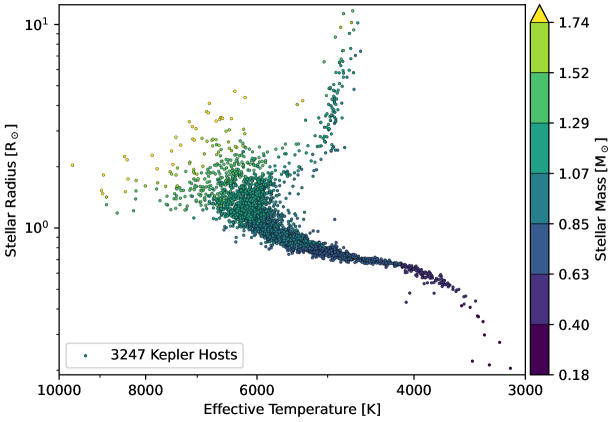
Figure 1: Stellar radius versus effective temperature for the Kepler host sample from 2, which used Gaia DR3 photometry, parallaxes, spectrophotometric metallicities, extinction maps, and isochrone fitting with isoclassify to determine fundamental stellar parameters. Stars are colored by their mass.

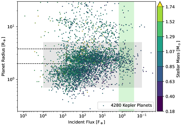
Figure 2: Planet radius versus incident flux for the Kepler planet sample from 2. Planets are colored according to the stellar mass of their host star, and those within the grey shaded region (0.7 $\mathrm{R_{\oplus}}$ $\leq$ $R_{\mathrm{p}}$ $\leq$ 5.1 $\mathrm{R_{\oplus}}$; 0.1 $\mathrm{F_{\oplus}}$ $\leq$ $F_{\mathrm{p}}$ $\leq$ 10⁴ $\mathrm{F_{\oplus}}$) will be included in the 3D planet radius gap measurement. We have also highlighted the hot sub-Neptunian desert within the dashed-box (2 $\mathrm{R_{\oplus}}$ $\leq$ $R_{\mathrm{p}}$ $\leq$ 3.8 $\mathrm{R_{\oplus}}$; $F_{\mathrm{p}}$ $>$ 650 $\mathrm{F_{\oplus}}$, Lundkvist et al., 2016) and the habitable zone as the green shaded region (0.25 $\mathrm{F_{\oplus}}$ $\leq$ $F_{\mathrm{p}}$ $\leq$ 1.50 $\mathrm{F_{\oplus}}$, Kane et al., 2016).

We take the stellar parameters from Berger et al. (2023) (hereafter 2), which used Gaia DR3 photometry, parallaxes, positions, and spectrophotometric metallicities (Gaia Collaboration et al., 2016, 2021; Lindegren et al., 2021a, b; Riello et al., 2021; Gaia Collaboration et al., 2022; Babusiaux et al., 2022; Creevey et al., 2022; Fouesneau et al., 2022; Andrae et al., 2022), and isoclassify (Huber et al., 2017; Berger et al., 2020a) in combination with the all-sky mwdust map (Bovy et al., 2016; Drimmel et al., 2003; Schlafly et al., 2014; Green et al., 2019) to derive stellar parameters from a custom-interpolated PARSEC model grid (Bressan et al., 2012) with YBC synthetic photometry (Chen et al., 2019). As described in 2, we fixed saturated photometry using the prescriptions in the appendix of Riello et al. (2021), fixed parallax zero points using the prescriptions of Lindegren et al. (2021b), and fixed the spectrophotometric metallicities using polynomial prescriptions (see 2) based on the California-Kepler Survey’s (CKS, Petigura et al., 2017) metallicities for overlapping stellar samples.

These new stellar parameters supersede those of Berger et al. (2020a) because we use Gaia DR3 photometry, which is more precise and homogeneous than KIC photometry (Brown et al., 2011). In addition, we use calibrated Gaia metallicities, which are available for more Kepler hosts and homogeneously derived unlike the heterogeneous combination of LAMOST (Ren et al., 2018), APOGEE (Abolfathi et al., 2018), and CKS (Petigura et al., 2017) metallicities. We also improved our M-dwarf stellar parameters by combining YBC synthetic photometry (Chen et al., 2019) and PARSEC models (Bressan et al., 2012) with the Mann et al. (2015, 2019) empirical relations.

In Figure 1, we plot the Kepler (NASA Exoplanet Archive, 2021) host star radii as a function of effective temperature, colored by stellar mass. The Kepler sample prioritized FGK dwarfs (Batalha et al., 2010; Wolniewicz et al., 2021), as the vast majority of Kepler host stars have $T_{\mathrm{eff}}$ from 4000–7000 K with corresponding masses from $\sim$0.6–1.3 $\mathrm{M_{\odot}}$. Consequently, there are few hosts with masses $>$ 1.74 $\mathrm{M_{\odot}}$ and $<$ 0.4 $\mathrm{M_{\odot}}$ or stellar radii $>$ 3 $\mathrm{R_{\odot}}$. We removed KOI 5635 (KIC 9178894) from further analysis, as it is an outlier at $T_{\mathrm{eff}}$ $\approx$ 12000 K with a mass of 3.4 $\mathrm{M_{\odot}}$.

In Figure 2, we plot the Kepler confirmed and candidate planet radii as a function of incident flux, also colored by host star mass. We find that most Kepler planets are smaller than 5 $\mathrm{R_{\oplus}}$, indicating their high occurrence rates throughout the Galaxy (Howard et al., 2010, 2012; Fressin et al., 2013; Petigura et al., 2013a, b; Dressing & Charbonneau, 2013; Hardegree-Ullman et al., 2019). In this paper, we focus on the 3702 planets within the grey box to isolate the populations of super-Earths below $\sim$2 $\mathrm{R_{\oplus}}$ and sub-Neptunes above $\sim$2 $\mathrm{R_{\oplus}}$ that are separated by the planet radius valley. In addition to the valley, we see, as in Berger et al. (2018b, 2020b), a hot-Jupiter inflation trend (Miller & Fortney, 2011; Thorngren et al., 2016; Grunblatt et al., 2017), planets within the hot sub-Neptunian desert (dashed box, Lundkvist et al., 2016), and planets in the habitable zone (green shaded region, Kane et al., 2016).

In order to preserve homogeneity in the derived planet parameters, we do not use K2 and TESS exoplanets, as Kepler, K2, and TESS used different transit-fitting pipelines. We chose Kepler because it has superior precision relative to K2 and TESS and $>$4000 planets.

3 Measuring the 3D Planet Radius Gap

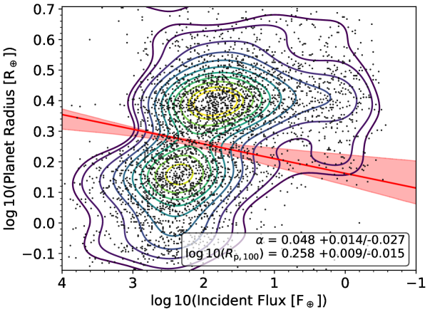
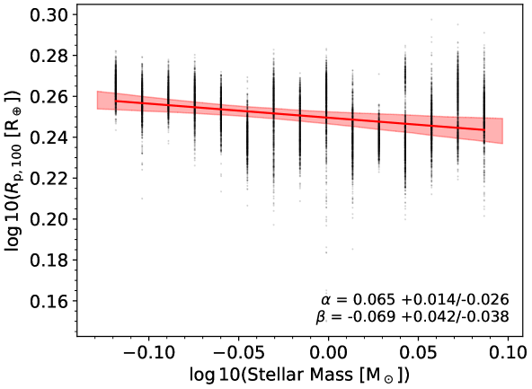
Figure 3: Methodology of measuring the planet radius gap in 3D. $Left$: $\log_{10}\left(\mathrm{Planet\ Radius}\right)$ versus $\log_{10}\left(\mathrm{Incident\ Flux}\right)$ at a mass slice of 1.00 $\mathrm{M_{\odot}}$. Contours represent a slice of the 3D KDE, while the dots represent planets re-drawn from the contours. We use gapfit (Loyd et al., 2020) and 1000 bootstrap simulations with replacement to determine the best-fit gap line, which is shown in solid red, with the 16th and 84th percentile ranges for each incident flux value as the shaded region above and below the line. The gap’s slope ($\alpha$) and intercept ($\log_{10}\left(R_{\mathrm{p,100}}\right)$) and their uncertainties for this individual mass slice are displayed at the bottom of the plot. $Right$: Best-fit line (red) to the 1000 bootstrapped $\log_{10}\left(R_{\mathrm{p,100}}\right)$ values (black circles) computed for each mass slice as in the left panel, as a function of $\log_{10}\left(\mathrm{Stellar\ Mass}\right)$. We have also plotted the 16th and 84th percentile ranges of this best-fit line as the red shaded region. In the right panel, we report $\alpha$ as the median and 16th and 84th percentiles of the 1000 gap slopes determined for each of the 15 stellar mass slices and $\beta$ as the slope (and 16th and 84th percentiles) of the red line in the right panel.

To measure the planet radius gap in 3D, we begin with the 3702 Kepler confirmed and candidate planets between 0.7–5.1 $\mathrm{R_{\oplus}}$ and 0.1–10⁴ $\mathrm{F_{\oplus}}$ with uncertainties smaller than their measured parameters and compute a 3D kernel density estimate (KDE) distribution in $\log_{10}\left(\mathrm{Planet\ Radius}\right)$, $\log_{10}\left(\mathrm{Incident\ Flux}\right)$, and $\log_{10}\left(\mathrm{Stellar\ Mass}\right)$ using fastKDE (O’Brien et al., 2014, 2016). We chose these bounds to contain roughly 95% of the observed planet population smaller than 7 $\mathrm{R_{\oplus}}$, center our analysis on super-Earths and sub-Neptunes, and maximize the KDE’s resolution of the planet radius gap without ignoring significant portions of the super-Earths and sub-Neptunes. Next, we follow the procedure of Rogers et al. (2021) by computing the mean stellar host mass ($\approx$ 0.99 $\mathrm{M_{\odot}}$) and host mass standard deviation ($\approx$ 0.23 $\mathrm{M_{\odot}}$) of the 3702 planets, and then split the 3D KDE data into 15 stellar mass slices, ranging in equal logarithmic steps from 0.76–1.22 $\mathrm{M_{\odot}}$.

For each of these mass slices in planet radius versus incident flux-space, we used gapfit (Loyd et al., 2020), which takes discrete data in any two-dimensional parameter space, computes a kernel density estimate along a line that separates the “gappy” data, minimizes the density along that line by varying the line’s slope and intercept, and then bootstraps with replacement n times to determine uncertainties in the best-fit line. We used the following initialization parameters: x0=2.0 (reference $\log_{10}\left(\mathrm{Incident\ Flux}\right)$ in the gap line equation), y0_guess=0.25 (an initial guess of the y-value of the gap at x0), m_guess=0.05 (an initial guess of the slope of the gap), sig=0.15 (kernel width for gapfit KDE), y0_rng=0.20 (the maximum by which the gap lines are allowed to deviate from y0), and n=1000 (number of bootstrap simulations with replacement). Because gapfit requires a discrete planet population, we drew 3702 planets in planet radius-incident flux-space based on the likelihood defined by our contours. The left panel of Figure 3 illustrates this procedure at an individual mass slice of 1 $\mathrm{M_{\odot}}$.

We repeated our gapfit procedure for each stellar mass slice, recording 1000 bootstrapped $\alpha_{i}$ values and intercept values ($\log R_{\mathrm{p,100},i}$), defined as the planet radius intersected by the best-fit gap line at 100 $\mathrm{F_{\oplus}}$, for each slice. Next, we plotted the intercept values for each slice as a function of $\log_{10}\left(\mathrm{Stellar\ Mass}\right)$, and then fit 1000 lines to this data, one for each bootstrap simulation. We then computed the median of the slopes of these 1000 lines to determine $\beta$ $\equiv$ $\left(\partial\log R_{\mathrm{gap}}/\partial\log M_{\star}\right)_{S}$ and used the 16th and 84th percentiles of the best-fit lines to determine typical uncertainties on $\beta$. We show this fit in the right plot of Figure 3.

To determine the full uncertainties on $\alpha$ and $\beta$, we ran 1000 separate Monte Carlo simulations of the observed population, drawing each planet’s radius, incident flux, and stellar mass values from a probability distribution defined by its radius, incident flux, and stellar mass and their corresponding uncertainties. We only kept simulated planets within the 0.7–5.1 $\mathrm{R_{\oplus}}$ and 0.1–10⁴ $\mathrm{F_{\oplus}}$ bounds, which resulted in 10–50 fewer planets per simulation than the 3702 observed planets. We chose these bounds to match our observed population analysis above, center the super-Earths and sub-Neptunes, and maximize the KDE’s resolution of the planet radius gap without ignoring significant portions of the simulated super-Earths and sub-Neptunes. We measured $\alpha$ and $\beta$ following the same procedure as above and as illustrated in Figure 3, recording 15000 unique $\alpha$ and 1000 unique $\beta$ values for each Monte Carlo simulation. Finally, we combined the 15 million $\alpha$ and 1 million unique $\beta$ values and computed the 16th, 50th, and 84th percentiles for each.

4 Results & Discussion

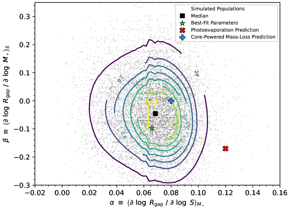
Figure 4: $\beta$ versus $\alpha$ for the Kepler planet population. The green star represents the observed distribution, while the filled red X and the filled blue plus represent the estimates of photoevaporation and core-powered mass-loss from (Rogers et al., 2021), respectively. The grey dots show the gap measurements resulting from 1000 Monte Carlo simulations with 15 stellar mass slices per simulation and 1000 bootstraps per mass slice for a total of 15 million $\alpha$ measurements and 1 million unique $\beta$ measurements. The contours display a Kernel Density Estimate (KDE) of the resulting probability distribution of the Monte Carlo simulations which account for the effects of finite sampling. Contours are labeled according to the fraction of simulations contained within them, with the 1$\sigma$ and 2$\sigma$ contours defined as containing 39.35% and 86.47% of the simulations, respectively (Wang et al., 2015). The black square is the median result of the simulations.

We plot our results in Figure 4. We measure $\alpha$ = 0.069${}^{+0.019}_{-0.023}$ and $\beta$ = $-$0.046${}^{+0.125}_{-0.117}$. The best-fit parameters occur within the contours representing the Monte Carlo simulations. The contours display higher variation on the $\beta$ axis than the $\alpha$ axis with a predominantly vertical orientation. The best-fit and median $\alpha$ values are smaller than predicted by both core-powered mass-loss and photoevaporation, while the best-fit and median $\beta$ values occur between the $\beta$ values predicted by core-powered mass-loss and photoevaporation. In addition, we find that the best-fit parameters are not centered within the contours, although they are well-within the uncertainties on both $\alpha$ and $\beta$ and can be explained by the random variations between simulations.

Given that the core-powered mass-loss prediction occurs at a contour corresponding to $\approx$ 0.7$\sigma$ and photoevaporation occurs at a contour corresponding to $\approx$ 2.8$\sigma$, we infer that core-powered mass-loss may be the dominant mechanism shaping the observed Kepler planet population, assuming our methodology is not biased (e.g. see discussion below). Another potential complication is that photoevaporation’s predicted $\beta$ is defined as the slope of the upper edge of the super-Earth population as a function of stellar mass at constant incident flux. We are unable to measure this quantity directly, as our measurement finds where the gap is deepest. Given the difference between a gap defined by the upper edge of the super-Earth population and where it is deepest, Rogers et al. (2021) illustrates that the deepest gap line produces a less-negative $\beta$ than the super-Earth upper edge gap line that photoevaporation predicts. However, even if we were to shift the photoevaporation estimate (red filled X) up to a larger $\beta$, it still would not occur at a lower sigma contour than core-powered mass-loss.

To ensure our simulations were not biased relative to the observed population, we ran similar simulations as in §3 but now reduced our uncertainties by factors of two and five. The resulting contours converged on the best-fit $\alpha$ and $\beta$ values with larger reductions in uncertainties, as expected. We also explored the effect of averaging the simulations together and computed contours that were virtually identical to the observed population. Therefore, we conclude that any biases between the simulated and best-fit parameters are introduced through the computation of the KDE from each simulated population and/or the subsequent determination of the best-fit gap line. However, these effects are small ($\Delta_{\alpha}$ = 0.004, $\Delta_{\beta}$ = 0.025) and well-within our reported uncertainties of $\sigma_{\alpha}$ $\approx$ 0.023 and $\sigma_{\beta}$ $\approx$ 0.130. As in Rogers et al. (2021), we wanted to ensure that we were using a sufficient number of stellar mass bins for computing $\alpha$ and $\beta$. Therefore, we tested 50 stellar mass bins in addition to the adopted 15 above and found no meaningful impact on our results.

We also performed the §3 procedure for the Berger et al. (2020b) Kepler planet sample to confirm our result is not sensitive to the exact stellar/planet properties. We computed $\alpha$ = 0.068${}^{+0.018}_{-0.023}$ and $\beta$ = 0.042${}^{+0.111}_{-0.109}$, which are statistically consistent with the $\alpha$ and $\beta$ values reported in this paper. In addition, we find that the predictions of core-powered mass-loss (corresponding contour $\approx$ 0.6$\sigma$) and photoevaporation (corresponding contour $\approx$ 3.1$\sigma$) for the Berger et al. (2020b) Kepler planet sample are at similar likelihoods as those studied here.

To determine whether our methodology introduced any biasing systematics, we tested a variety of gap determination methods and found some discrepancies. We used four different gap determination methods, detailed below, which differ solely by their determination of the best-fit gap line and the corresponding slope ($\alpha_{i}$) as a function of incident flux and intercept ($\log R_{\mathrm{p,100},i}$) for each mass slice. Once each method has determined its $\alpha_{i}$ and $\log R_{\mathrm{p,100},i}$ values for each mass slice $i$, the determination of $\alpha$ and $\beta$ follows from the description in §3.

1. The Petigura et al. (2022) methodology, which (1) draws a number of vertical lines spanning the gap as a function of incident flux, (2) finds the relative minimum density along those lines, and (3) fits a line to those minimum density points along each line.

2. A modified Petigura et al. (2022) methodology, where instead of drawing vertical lines, we draw a line between the peaks of the super-Earth and sub-Neptune populations and then draw corresponding parallel lines which span the gap. We use the same density arguments as in method 1 to determine the points on each line to fit.

3. The Rogers et al. (2021) methodology, which relies on minimizing the sum of the KDE along the gap line.

4. Our gapfit methodology, which we detailed in §3 above.

We found that while methodologies 1 and 3 produced similar results and 2 and 4 produced similar results, comparisons between the pairs produced systematically different results. Interestingly, we found systematically larger $\alpha$ values using the vertical lines of Petigura et al. (2022) than if we had repeated the same procedure with diagonal lines connecting the sub-Neptune and super-Earth peaks. This suggests that the methods dependent on drawing lines to define the gap as a function of incident flux are inherently dependent on the exact orientation of the lines drawn. In addition, the Rogers et al. (2021) method (method 3) relies on minimizing the sum of the KDE along the gap line, although we found that the method failed occasionally depending on the exact simulated planet population. Upon inspection, both gap line orientation methods appeared to fit the gap equally well, so we concluded that we needed a method that would capture this uncertainty.

Hence, we decided to use gapfit (Loyd et al., 2020), which, similar to Rogers et al. (2021), attempts to minimize the sum of the KDE along the gap line and also bootstraps with replacement to sample the gap line uncertainties for each mass slice of each Monte Carlo-simulated planet population. We also found that our method is robust and rarely failed to produce $\alpha$ and $\beta$ estimates after hundreds of simulations. Regardless, we produce systematically smaller $\alpha$ values than those measured by Rogers et al. (2021), which results in our $\gtrsim$2$\sigma$ preference for core-powered mass-loss over photoevaporation as the mechanism sculpting the Kepler exoplanet radius gap. Interestingly, Ho & Van Eylen (2023) used Kepler short cadence observations and yet another independent gap fitting approach to find $\alpha$ and $\beta$ values that are more consistent with core-powered mass-loss than photoevaporation.

We note that the $expectation$ values of $\alpha$ and $\beta$ for the two theories determined by Rogers et al. (2021), to which we compare our results, are not the same as those $measured$ by Rogers et al. (2021). However, we caution that any measurement of the 3D planet radius gap may be the result of systematics present in the chosen gap-determination method, given the discrepancies between our measurements and those of Rogers et al. (2021) and Petigura et al. (2022). This therefore motivates the use of an unbiased gap measurement methodology and a need for more precise and accurate planet radii.

5 Conclusion

In this paper, we used the latest Kepler host stellar properties with Gaia DR3 constraints from 2 to compute the slope of the Kepler planet radius gap as a function of incident flux and stellar mass. We aimed to differentiate between the mechanisms of core-powered mass-loss and photoevaporation for Kepler planets.

We measure $\alpha$ = 0.069${}^{+0.019}_{-0.023}$ and $\beta$ = $-$0.046${}^{+0.125}_{-0.117}$, which are $\gtrsim$2$\sigma$ more consistent with the Rogers et al. (2021) predictions of core-powered mass-loss ($\alpha$ $\approx$ 0.08, $\beta$ $\approx$ 0.00) than photoevaporation ($\alpha$ $\approx$ 0.12, $\beta$ $\approx$ –0.17) and consistent with Ho & Van Eylen (2023). While photoevaporation predicts a more-negative $\beta$ than is possible to measure due to photoevaporation’s gap definition as the upper edge of the super-Earth population rather than where the gap is deepest, shifting the photoevaporation prediction to a larger $\beta$ does not change our conclusion.

We caution that the measurement of the exoplanet radius gap is dependent on the exact methodology used. We found that our methodology based on gapfit (Loyd et al., 2020) produced systematically smaller $\alpha$ values relative to the Rogers et al. (2021) and Petigura et al. (2022) methods, although they are consistent within uncertainties. Rogers et al. (2021) measures an $\alpha$ = 0.10${}^{+0.03}_{-0.02}$ that is consistent with the theoretical predictions of both core-powered mass-loss ($\alpha$ $\approx$ 0.08) and photoevaporation ($\alpha$ $\approx$ 0.12), while our systematically smaller $\alpha$ = 0.069${}^{+0.019}_{-0.023}$ favors core-powered mass-loss over photoevaporation. Our measured $\beta$ = $-$0.046${}^{+0.125}_{-0.117}$ is consistent with both theories.

While adding more planets from K2 and TESS may improve our understanding of planet demographics, the large number and exquisite precision of Kepler planet radii represent the ideal sample for constraining $\alpha$ and $\beta$ and hence the planet radius gap. This study therefore motivates a systematic re-fitting of Kepler planet transits, leveraging the latest eccentricity priors for single and multi-planet systems and mean stellar densities to better constrain $\frac{R_{\mathrm{p}}}{R_{\star}}$ values (Petigura, 2020). In turn, this will increase the accuracy and precision of planet radii and hence our measurements of the planet radius gap. These new measurements may enable us to differentiate between the theories of core-powered mass-loss and photoevaporation for the Kepler sample once and for all.

Exoplanet Archive

References

- Abolfathi et al. (2018) Abolfathi, B., Aguado, D. S., Aguilar, G., et al. 2018, ApJS, 235, 42, doi: 10.3847/1538-4365/aa9e8a
- Andrae et al. (2022) Andrae, R., Fouesneau, M., Sordo, R., et al. 2022, arXiv e-prints, arXiv:2206.06138. https://arxiv.org/abs/2206.06138
- Babusiaux et al. (2022) Babusiaux, C., Fabricius, C., Khanna, S., et al. 2022, arXiv e-prints, arXiv:2206.05989. https://arxiv.org/abs/2206.05989
- Batalha et al. (2010) Batalha, N. M., Borucki, W. J., Koch, D. G., et al. 2010, ApJ, 713, L109, doi: 10.1088/2041-8205/713/2/L109
- Berger et al. (2018a) Berger, T. A., Howard, A. W., & Boesgaard, A. M. 2018a, ApJ, 855, 115, doi: 10.3847/1538-4357/aab154
- Berger et al. (2018b) Berger, T. A., Huber, D., Gaidos, E., & van Saders, J. L. 2018b, ApJ, 866, 99, doi: 10.3847/1538-4357/aada83
- Berger et al. (2020a) Berger, T. A., Huber, D., van Saders, J. L., et al. 2020a, AJ, 159, 280, doi: 10.3847/1538-3881/159/6/280
- Berger et al. (2020b) Berger, T. A., Huber, D., Gaidos, E., van Saders, J. L., & Weiss, L. M. 2020b, AJ, 160, 108, doi: 10.3847/1538-3881/aba18a
- Borucki et al. (2010) Borucki, W. J., Koch, D., Basri, G., et al. 2010, Science, 327, 977, doi: 10.1126/science.1185402
- Bovy et al. (2016) Bovy, J., Rix, H.-W., Green, G. M., Schlafly, E. F., & Finkbeiner, D. P. 2016, ApJ, 818, 130, doi: 10.3847/0004-637X/818/2/130
- Bressan et al. (2012) Bressan, A., Marigo, P., Girardi, L., et al. 2012, MNRAS, 427, 127, doi: 10.1111/j.1365-2966.2012.21948.x
- Brown et al. (2011) Brown, T. M., Latham, D. W., Everett, M. E., & Esquerdo, G. A. 2011, AJ, 142, 112, doi: 10.1088/0004-6256/142/4/112
- Chen et al. (2019) Chen, Y., Girardi, L., Fu, X., et al. 2019, A&A, 632, A105, doi: 10.1051/0004-6361/201936612
- Claytor et al. (2020) Claytor, Z. R., van Saders, J. L., Santos, Â. R. G., et al. 2020, ApJ, 888, 43, doi: 10.3847/1538-4357/ab5c24
- Cloutier & Menou (2020) Cloutier, R., & Menou, K. 2020, AJ, 159, 211, doi: 10.3847/1538-3881/ab8237
- Creevey et al. (2022) Creevey, O. L., Sordo, R., Pailler, F., et al. 2022, arXiv e-prints, arXiv:2206.05864. https://arxiv.org/abs/2206.05864
- David et al. (2021) David, T. J., Contardo, G., Sandoval, A., et al. 2021, AJ, 161, 265, doi: 10.3847/1538-3881/abf439
- Dressing & Charbonneau (2013) Dressing, C. D., & Charbonneau, D. 2013, ApJ, 767, 95, doi: 10.1088/0004-637X/767/1/95
- Drimmel et al. (2003) Drimmel, R., Cabrera-Lavers, A., & López-Corredoira, M. 2003, A&A, 409, 205, doi: 10.1051/0004-6361:20031070
- Fouesneau et al. (2022) Fouesneau, M., Frémat, Y., Andrae, R., et al. 2022, arXiv e-prints, arXiv:2206.05992. https://arxiv.org/abs/2206.05992
- Fressin et al. (2013) Fressin, F., Torres, G., Charbonneau, D., et al. 2013, ApJ, 766, 81, doi: 10.1088/0004-637X/766/2/81
- Fulton & Petigura (2018) Fulton, B. J., & Petigura, E. A. 2018, AJ, 156, 264, doi: 10.3847/1538-3881/aae828
- Fulton et al. (2017) Fulton, B. J., Petigura, E. A., Howard, A. W., et al. 2017, AJ, 154, 109, doi: 10.3847/1538-3881/aa80eb
- Gaia Collaboration et al. (2016) Gaia Collaboration, Prusti, T., de Bruijne, J. H. J., et al. 2016, A&A, 595, A1, doi: 10.1051/0004-6361/201629272
- Gaia Collaboration et al. (2018) Gaia Collaboration, Brown, A. G. A., Vallenari, A., et al. 2018, A&A, 616, A1, doi: 10.1051/0004-6361/201833051
- Gaia Collaboration et al. (2021) —. 2021, A&A, 649, A1, doi: 10.1051/0004-6361/202039657
- Gaia Collaboration et al. (2022) Gaia Collaboration, Vallenari, A., Brown, A. G. A., et al. 2022, arXiv e-prints, arXiv:2208.00211. https://arxiv.org/abs/2208.00211
- Ginzburg et al. (2016) Ginzburg, S., Schlichting, H. E., & Sari, R. 2016, ApJ, 825, 29, doi: 10.3847/0004-637X/825/1/29
- Ginzburg et al. (2018) —. 2018, MNRAS, 476, 759, doi: 10.1093/mnras/sty290
- Green et al. (2019) Green, G. M., Schlafly, E., Zucker, C., Speagle, J. S., & Finkbeiner, D. 2019, ApJ, 887, 93, doi: 10.3847/1538-4357/ab5362
- Grunblatt et al. (2017) Grunblatt, S. K., Huber, D., Gaidos, E., et al. 2017, AJ, 154, 254, doi: 10.3847/1538-3881/aa932d
- Gupta & Schlichting (2019) Gupta, A., & Schlichting, H. E. 2019, MNRAS, 487, 24, doi: 10.1093/mnras/stz1230
- Gupta & Schlichting (2020) —. 2020, MNRAS, 493, 792, doi: 10.1093/mnras/staa315
- Hardegree-Ullman et al. (2019) Hardegree-Ullman, K. K., Cushing, M. C., Muirhead, P. S., & Christiansen, J. L. 2019, AJ, 158, 75, doi: 10.3847/1538-3881/ab21d2
- Hardegree-Ullman et al. (2020) Hardegree-Ullman, K. K., Zink, J. K., Christiansen, J. L., et al. 2020, ApJS, 247, 28, doi: 10.3847/1538-4365/ab7230
- Harris et al. (2020) Harris, C. R., Millman, K. J., van der Walt, S. J., et al. 2020, Nature, 585, 357, doi: 10.1038/s41586-020-2649-2
- Ho & Van Eylen (2023) Ho, C. S. K., & Van Eylen, V. 2023, arXiv e-prints, arXiv:2301.04062. https://arxiv.org/abs/2301.04062
- Howard et al. (2010) Howard, A. W., Marcy, G. W., Johnson, J. A., et al. 2010, Science, 330, 653, doi: 10.1126/science.1194854
- Howard et al. (2012) Howard, A. W., Marcy, G. W., Bryson, S. T., et al. 2012, ApJS, 201, 15, doi: 10.1088/0067-0049/201/2/15
- Huber et al. (2017) Huber, D., Zinn, J., Bojsen-Hansen, M., et al. 2017, ApJ, 844, 102, doi: 10.3847/1538-4357/aa75ca
- Hunter (2007) Hunter, J. D. 2007, Computing In Science & Engineering, 9, 90, doi: 10.1109/MCSE.2007.55
- Johnson et al. (2017) Johnson, J. A., Petigura, E. A., Fulton, B. J., et al. 2017, AJ, 154, 108, doi: 10.3847/1538-3881/aa80e7
- Kane et al. (2016) Kane, S. R., Hill, M. L., Kasting, J. F., et al. 2016, ApJ, 830, 1, doi: 10.3847/0004-637X/830/1/1
- Lee (2019) Lee, E. J. 2019, ApJ, 878, 36, doi: 10.3847/1538-4357/ab1b40
- Lee & Chiang (2016) Lee, E. J., & Chiang, E. 2016, ApJ, 817, 90, doi: 10.3847/0004-637X/817/2/90
- Lee et al. (2014) Lee, E. J., Chiang, E., & Ormel, C. W. 2014, ApJ, 797, 95, doi: 10.1088/0004-637X/797/2/95
- Lindegren et al. (2018) Lindegren, L., Hernández, J., Bombrun, A., et al. 2018, A&A, 616, A2, doi: 10.1051/0004-6361/201832727
- Lindegren et al. (2021a) Lindegren, L., Klioner, S. A., Hernández, J., et al. 2021a, A&A, 649, A2, doi: 10.1051/0004-6361/202039709
- Lindegren et al. (2021b) Lindegren, L., Bastian, U., Biermann, M., et al. 2021b, A&A, 649, A4, doi: 10.1051/0004-6361/202039653
- Loyd et al. (2020) Loyd, R. O. P., Shkolnik, E. L., Schneider, A. C., et al. 2020, ApJ, 890, 23, doi: 10.3847/1538-4357/ab6605
- Lundkvist et al. (2016) Lundkvist, M. S., Kjeldsen, H., Albrecht, S., et al. 2016, Nature Communications, 7, 11201, doi: 10.1038/ncomms11201
- Mann et al. (2015) Mann, A. W., Feiden, G. A., Gaidos, E., Boyajian, T., & von Braun, K. 2015, ApJ, 804, 64, doi: 10.1088/0004-637X/804/1/64
- Mann et al. (2019) Mann, A. W., Dupuy, T., Kraus, A. L., et al. 2019, ApJ, 871, 63, doi: 10.3847/1538-4357/aaf3bc
- McKinney (2010) McKinney, W. 2010, in Proceedings of the 9th Python in Science Conference, ed. S. van der Walt & J. Millman, 51 – 56
- Miller & Fortney (2011) Miller, N., & Fortney, J. J. 2011, ApJ, 736, L29, doi: 10.1088/2041-8205/736/2/L29
- Misener & Schlichting (2021) Misener, W., & Schlichting, H. E. 2021, MNRAS, 503, 5658, doi: 10.1093/mnras/stab895
- NASA Exoplanet Archive (2021) NASA Exoplanet Archive. 2021, Kepler Objects of Interest Cumulative Table, Version: 2021-11-05 16:03, NExScI-Caltech/IPAC, doi: 10.26133/NEA4
- Owen & Murray-Clay (2018) Owen, J. E., & Murray-Clay, R. 2018, MNRAS, 480, 2206, doi: 10.1093/mnras/sty1943
- Owen & Wu (2013) Owen, J. E., & Wu, Y. 2013, ApJ, 775, 105, doi: 10.1088/0004-637X/775/2/105
- Owen & Wu (2016) —. 2016, ApJ, 817, 107, doi: 10.3847/0004-637X/817/2/107
- Owen & Wu (2017) —. 2017, ApJ, 847, 29, doi: 10.3847/1538-4357/aa890a
- O’Brien et al. (2014) O’Brien, T. A., Collins, W. D., Rauscher, S. A., & Ringler, T. D. 2014, Computational Statistics & Data Analysis, 79, 222, doi: https://doi.org/10.1016/j.csda.2014.06.002
- O’Brien et al. (2016) O’Brien, T. A., Kashinath, K., Cavanaugh, N. R., Collins, W. D., & O’Brien, J. P. 2016, Computational Statistics & Data Analysis, 101, 148, doi: https://doi.org/10.1016/j.csda.2016.02.014
- Petigura (2020) Petigura, E. A. 2020, AJ, 160, 89, doi: 10.3847/1538-3881/ab9fff
- Petigura et al. (2013a) Petigura, E. A., Marcy, G. W., & Howard, A. W. 2013a, ApJ, 770, 69, doi: 10.1088/0004-637X/770/1/69
- Petigura et al. (2013b) Petigura, E. A., Howard, A. W., & Marcy, G. W. 2013b, PNAS, 110, 19175, doi: 10.1088/0004-637X/770/1/69
- Petigura et al. (2017) Petigura, E. A., Howard, A. W., Marcy, G. W., et al. 2017, AJ, 154, 107, doi: 10.3847/1538-3881/aa80de
- Petigura et al. (2018) Petigura, E. A., Marcy, G. W., Winn, J. N., et al. 2018, AJ, 155, 89, doi: 10.3847/1538-3881/aaa54c
- Petigura et al. (2022) Petigura, E. A., Rogers, J. G., Isaacson, H., et al. 2022, AJ, 163, 179, doi: 10.3847/1538-3881/ac51e3
- Ren et al. (2018) Ren, J. J., Rebassa-Mansergas, A., Parsons, S. G., et al. 2018, MNRAS, 477, 4641, doi: 10.1093/mnras/sty805
- Riello et al. (2021) Riello, M., De Angeli, F., Evans, D. W., et al. 2021, A&A, 649, A3, doi: 10.1051/0004-6361/202039587
- Rogers et al. (2021) Rogers, J. G., Gupta, A., Owen, J. E., & Schlichting, H. E. 2021, arXiv e-prints, arXiv:2105.03443. https://arxiv.org/abs/2105.03443
- Rogers & Owen (2021) Rogers, J. G., & Owen, J. E. 2021, MNRAS, 503, 1526, doi: 10.1093/mnras/stab529
- Sandoval et al. (2021) Sandoval, A., Contardo, G., & David, T. J. 2021, ApJ, 911, 117, doi: 10.3847/1538-4357/abea9e
- Schlafly et al. (2014) Schlafly, E. F., Green, G., Finkbeiner, D. P., et al. 2014, ApJ, 789, 15, doi: 10.1088/0004-637X/789/1/15
- Schlichting et al. (2015) Schlichting, H. E., Sari, R., & Yalinewich, A. 2015, Icarus, 247, 81, doi: 10.1016/j.icarus.2014.09.053
- Taylor (2005) Taylor, M. B. 2005, in Astronomical Society of the Pacific Conference Series, Vol. 347, Astronomical Data Analysis Software and Systems XIV, ed. P. Shopbell, M. Britton, & R. Ebert, 29
- Thorngren et al. (2016) Thorngren, D. P., Fortney, J. J., Murray-Clay, R. A., & Lopez, E. D. 2016, ApJ, 831, 64, doi: 10.3847/0004-637X/831/1/64
- Van Eylen et al. (2018) Van Eylen, V., Agentoft, C., Lundkvist, M. S., et al. 2018, MNRAS, 479, 4786, doi: 10.1093/mnras/sty1783
- Virtanen et al. (2020) Virtanen, P., Gommers, R., Oliphant, T. E., et al. 2020, Nature Methods, 17, 261, doi: https://doi.org/10.1038/s41592-019-0686-2
- Wang et al. (2015) Wang, B., Shi, W., & Miao, Z. 2015, PLOS ONE, 10, doi: 10.1371/journal.pone.0118537
- Wolniewicz et al. (2021) Wolniewicz, L. M., Berger, T. A., & Huber, D. 2021, AJ, 161, 231, doi: 10.3847/1538-3881/abee1d
- Wu (2019) Wu, Y. 2019, ApJ, 874, 91, doi: 10.3847/1538-4357/ab06f8
- Zink et al. (2021) Zink, J. K., Hardegree-Ullman, K. K., Christiansen, J. L., et al. 2021, AJ, 162, 259, doi: 10.3847/1538-3881/ac2309