On the Initialisation of Wide Low-Rank Feedforward Neural Networks

Abstract

The edge-of-chaos dynamics of wide randomly initialized low-rank feedforward networks are analyzed. Formulae for the optimal weight and bias variances are extended from the full-rank to low-rank setting and are shown to follow from multiplicative scaling. The principle second order effect, the variance of the input-output Jacobian, is derived and shown to increase as the rank to width ratio decreases. These results inform practitioners how to randomly initialize feedforward networks with a reduced number of learnable parameters while in the same ambient dimension, allowing reductions in the computational cost and memory constraints of the associated network.

1 Introduction

Neural networks being applied to new settings, limiting transfer learning, are typically initialized with i.i.d. random entries. The edge-of-chaos theory of (Poole et al., 2016) determine the appropriate scaling of the weight matrices and biases so that intermediate layer representations (1) and the median of the input-output Jacobian’s spectra (10) are to first order independent of the layer. Without this normalization there is typically an exponential growth in the magnitude of these intermediate representations and gradients as they progress between layers of the network; such a disparity of scale inhibits the early training of the network (Glorot & Bengio, 2010).

For instance, consider an untrained fully connected neural network whose weights and biases are set to be respectively identically and independently distributed with respect to a Gaussian distributions: $W^{(l)}_{ij}\sim\mathcal{N}(0,\frac{\sigma^{2}_{W}}{N_{l-1}})$, $b^{(l)}_{i}\sim\mathcal{N}(0,\sigma^{2}_{b})$ with $N_{l}$ the width at layer $l$. Starting such a network, with nonlinear activation $\phi:\mathbb{R}\to\mathbb{R}$, from an input vector $z^{0}:=x^{0}\in\mathbb{R}^{N_{0}}$, the data propagation is then given by the following equations,

$$h_{j}^{(l)}=\sum\limits_{k=1}^{N_{l-1}}W^{(l)}_{jk}z^{(l)}_{k}+b^{(l)}_{j},\qquad z^{(l)}_{k}=\phi(h^{(l-1)}_{k})$$ (1)

where we call $h^{(l)}$ the preactivation vector at layer $l$.

It has been shown by (Poole et al., 2016) that the preactivation vectors $h^{l}$ have geometric properties of length $q^{l}:=N_{l}^{-1}\left(h^{l}\right)^{T}h^{l}$ and the pairwise covariance $q^{l}_{12}:=N_{l}^{-1}\left(h_{1}^{l}\right)^{T}h_{2}^{l}$ of two inputs $x^{0,1}$ and $x^{0,2}$ which propagate through the network according to functions of the network entries’ variances and nonlinear activation $(\sigma_{b},\sigma_{W},\phi)$. These propagation maps were computed by (Poole et al., 2016) in the limiting setting of infinitely wide networks and either i.i.d. Gaussian entries or scaled randomly drawn orthnormal matrices. Here we extend this setting to their low-rank analogous.

Consider rank $r_{l}:=\gamma_{l}N_{l}$ weight matrices, $W^{(l)}\in\mathbb{R}^{N_{l}\times N_{l-1}}$, formed as

$$W^{(l)}_{ij}=\sum\limits_{k=1}^{r_{l}}\alpha_{k,j}^{(l)}(C_{k}^{l})_{i},$$ (2)

where the scalars $\left(\alpha^{(l)}_{k,i}\right)_{1\leq i\leq N_{l-1}}\in\mathbb{R}\overset{\text{iid}}{\sim}\mathcal{N}(0,\frac{\sigma_{\alpha}^{2}}{N_{l-1}})$ and the columns $C^{(l)}_{1},\dots,C^{(l)}_{r_{l}}$ are drawn jointly as the matrix $C^{(l)}:=[C^{(l)}_{1},\dots,C^{(l)}_{r_{l}}]\in\mathbb{R}^{N_{l}\times r_{l}}$ from the Grassmannian of rank $r$ matrices with orthonormal columns having zero mean and variance $1/N_{l}$. Similarly, consider bias vectors within the same column span as $W^{(l)}$, given by $b^{(l)}(C^{(l)}_{1}+\dots+C^{(l)}_{r_{l}})$, where $b^{(l)}\in\mathbb{R}\sim\mathcal{N}(0,\sigma_{b}^{2})$. It is shown in Appendix A.2 that, in the large width limit, the preactivation vector $h^{(l)}$ follows a Gaussian distribution over the $r-$dimensional column span of $W^{(l)}$ with a non-diagonal covariance; this differs from the full rank setting in (Poole et al., 2016) where the entries in (1) are independent.

We extend the pre-activation length and correlation maps to this low-rank setting:

$$q^{l} =\gamma_{l} \bigg{(}\sigma^{2}_{\alpha}\int_{\mathbb{R}}\phi^{2}(\sqrt{q^{l-1}}z)Dz+\sigma_{b}^{2}\bigg{)}$$ (3)

$$:=\mathcal{V}(q^{(l-1)}|\sigma_{\alpha},\sigma_{b},\gamma_{l})$$ (4)

where $Dz:=\frac{1}{\sqrt{2\pi}}e^{-\frac{z^{2}}{2}}dz$ is the Gaussian probability measure, and

$$q^{l}_{12} =\gamma_{l}\bigg{(}\sigma^{2}_{\alpha}\int_{\mathbb{R}^{2}}\phi(u_{1})\phi(u_{2})Dz_{1}Dz_{2}+\sigma^{2}_{b}\bigg{)},$$ (5)

$$:=\mathcal{C}(q_{ab}^{l-1},q_{aa}^{l-1},q_{bb}^{l-1}|\sigma_{\alpha},\sigma_{b},\gamma_{l})$$ (6)

with $u_{1}=\sqrt{q^{l-1}_{11}}z_{1},u_{2}=\sqrt{q^{l-1}_{22}}(c_{12}^{l-1}z_{1}+\sqrt{1-(c_{12}^{l-1})^{2}}z_{2}$ and

$$c_{12}^{l}=q_{12}^{l}(q_{11}^{l}q_{22}^{l})^{-\frac{1}{2}}.$$ (7)

Equations (3) and (5) are derived in Section A.3 and Section A.4 respectively. These equations exactly recover the equations by (Poole et al., 2016) when $\gamma_{l}=1$, and show that by appropriately rescaling $\sigma_{2}^{2}$ and $\sigma_{b}^{2}$ by $\gamma_{r}$ the low-rank maps remain consistent with the full rank setting.

These two mappings (3) and (5) are functions of the network entries variances, the rank at each layer $\gamma_{l}$ and the nonlinear activation $(\sigma_{b},\sigma_{W},\gamma_{l},\phi)$ which determine the existence of eventual stable fixed points of $q^{l}$ and $q^{l}_{ab}$ as well as the dynamics they follow through the network.

The dominant quantity determining the dynamics of the network is

$$\chi_{\gamma} :=\gamma\sigma^{2}_{\alpha}\int_{\mathbb{R}}\bigg{(}\phi^{\prime}(\sqrt{q^{*}}z)\bigg{)}^{2}Dz$$ (8)

which is equal to two fundamental quantities. First, $\chi_{\gamma}$ is equal to the gradient of the correlation function (7) evaluated at correlation $c_{12}^{l}=1$,

$$\chi_{\gamma}=\frac{\partial c^{l}_{12}}{\partial c^{l-1}_{12}}|_{c^{l-1}_{12}=1}$$ (9)

A detailed derivation of the equivalence of (8) and (9) is given in Appendix A.5. When there exists a fixed point $q^{*}$ such that $\mathcal{V}(q^{*})=q^{*}$, and $\chi<1$, then inputs with small initial correlation converge to correlation 1 at an exponential rate; this phase is referred to as ordered. Alternatively, when $\chi>1$ the fixed point $c^{*}=1$ becomes unstable, meaning that an input and its arbitrarily small perturbation have correlation $q^{l}_{ab}$ decreasing with layers; this is referred to as the chaotic phase due to all nearby points on a data manifold diverging as they progress through the network. In the ordered phase, the output function of the network is constant whereas in the chaotic phase it is non-smooth everywhere.

In both cases ($\chi>1$ or $\chi<1$), in (Schoenholz et al., 2016), the mappings $\mathcal{V}$ and $\frac{1}{q^{*}}\mathcal{C}$ are shown to converge exponentially fast to their fixed point, when they exist. Therefore, the data geometry is quickly lost as it is propagated through layers. The boundary between these phases, where $\chi=1$, is referred to as the edge-of-chaos and determines the scaling of $(\sigma_{w},\sigma_{b},\gamma_{l})$, as functions of nonlinear activation $\phi(\cdot)$, which ensures a sub-exponential asymptotic behaviour of these maps towards their fixed point and thus a deeper data propagation along layers which facilitates early training of the network.

Second, the quantity $\chi_{\gamma}$ in (8) is equal to the median singular value of the the matrix $D^{(l)}W^{(l)}$ where $D^{(l)}$ is the diagonal matrix with at layer $l$ with entries $D_{ii}^{(l)}=\phi^{\prime}(h_{i}^{l})$; for details see Appendix A.9. Defining the Jacobian matrix $J\in\mathbb{R}^{N_{L}\times N_{0}}$ of the input-output map as

$$J:=\frac{\partial z^{L}}{\partial z^{0}}=\prod_{l=1}^{L}D^{(l)}W^{(l)},$$ (10)

we see that the average singular value of $J$ is equal to $\chi_{\gamma}^{L}$. If $\chi_{\gamma}=1$ the average singular value of $J$ is fixed at 1 throughout the network, while if $\chi_{\gamma}$ is greater than or less than 1 the average singular value deviates from 1 at an exponential rate. Further note that the growth of a perturbation from a layer to the following one is given by the average squared singular value of $D^{(l)}W^{(l)}$.

1.1 Main contributions

This manuscript extends the edge-of-chaos analysis of random feed-forward networks to the setting of low-rank matrices, following the work of (Poole et al., 2016). This work is motivated by the recent challenges faced to store in memory the constantly growing number of parameters used to train large Deep Learning models, see (Price & Tanner, 2022) and references therein.

As shown in equations (3), (6), and (8), despite the dependence between entries in the low-rank weight matrices (2), that the edge-of-chaos curve defined by $\chi_{\gamma}=1$ can be retained by scaling the weight and bias variances $\sigma_{w}^{2}$ and $\sigma_{b}^{2}$ respectively by the ratio of the weight matrix rank $r_{l}$ to layer width $\gamma_{l}:=r_{l}/N_{l}$, see Figure 1 and contrast with Figure 10. That is, a simple re-scaling retains the dominant first order dynamics of a feedforward network when the weight matrices are initialized to be low-rank.

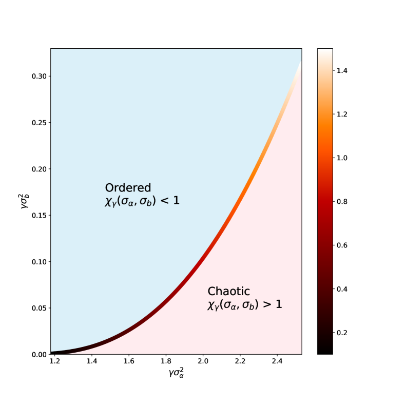
Figure 1: Edge of Chaos curve of a low-rank neural network where the rank is proportional to the width by a factor $\gamma$ and nonlinear activation $\phi(x)=tanh(x)$ . The plot is generated with $\gamma=\frac{1}{4}$, where the axis are rescaled by $\gamma$.

In Section 2 we show that additional first order dynamics are similarly modified through a multiplicative scaling by the rank to width factor $\gamma_{l}=r_{l}/N_{l}$. In particular, we demonstrate the role of $\gamma_{l}$ on the length and correlation depth scale as well as the training gradient vectors.

However, in Section 3 we show that important second order properties of the dynamics, specifically the variance of the singular values of the input-output Jacobian given in (10), is modified by the reduced rank in a way that cannot be overcome with simple re-scaling. This result alerts practitioners to anticipated greater variability in training low-rank weight matrices and suggests that methods to reduce the variance of the spectrum may be increasingly important in this setting, see (Murray et al., 2021).

The manuscript then concludes with numerical experiments in Section 4 which demonstrate that empirical measurements on the Jacobian are consistent with the established formula and a brief summary and future work in Section 5.

2 Network dynamics and data propagation

The parameter $\chi_{\gamma}$ further controls the length and correlation depth scaling as well as the relative magnitude of training gradients computed via back-propagration for the sum-of-squares loss function.

2.1 Depth scales a functions of $\chi_{\gamma}$

The role of $\chi_{\gamma}$ on the achievable depth scale was pioneered by (Schoenholz et al., 2016) for full-rank feedforward networks. In this subsection we extend their results to the low-rank setting with the suitably adapted spectral mean $\chi_{\gamma}$ given in (8).

2.1.1 Length depth scale

Assuming there exists a fixed point $q^{*}$ such that $\mathcal{V}(q^{*})=q^{*}$, then the dynamics of $\mathcal{V}(q)$ can be linearized around $q^{*}$ to obtain stability conditions and a rate of decay which determine how deeply data can propagate through the network before converging towards the fixed point. Following the computations done in (Schoenholz et al., 2016), setting a perturbation around the fixed point $q^{*}+\epsilon_{l}$, then around the fixed point, $\epsilon_{l}$ evolves as $e^{-\frac{l}{\xi_{q,\gamma}}}$, when $\gamma_{l}=^{\prime}gamma$ is fixed along layers and we define the following quantities,

$$\xi_{q,\gamma}^{-1} :=-\log\bigg{(}\chi_{\gamma}+\gamma\sigma^{2}_{\alpha}\int Dz\phi^{\prime\prime}(\sqrt{q^{*}}z)\phi(\sqrt{q^{*}}z)\bigg{)}.$$

Details are given in Section A.6. Given that $\gamma\in(0,1]$, we can see the convergence gets faster towards the fixed point when increasing $\gamma$. Note that when $\gamma\sigma^{2}_{\alpha}=\sigma^{2}_{W}$, we recover the results of a full-rank feedforward neural network in (Schoenholz et al., 2016).

2.1.2 Correlation depth scale

Similarly, we compute the dynamical evolution of the correlation map around its fixed point by considering a perturbation $\epsilon_{l}$ and we obtain that (see Section A.7), when all the ranks are set to be proportional to the width with the same coefficient of proportionality $\gamma_{l}=\gamma$ at any layer $l$, then the perturbation vanishes exponentially fast $\epsilon_{l}=\mathcal{O}(e^{-\frac{l}{\xi_{q,\gamma}}})$ where

$$\xi_{c,\gamma}^{-1} :=-\log\big{(}\chi_{\gamma}\big{)}.$$

We recover that the correlation depth scale diverges to $+\infty$ when $\chi_{\gamma}\to 1$, yielding again the key role of this quantity, even in the low-rank case. As $\gamma\in(0,1]$, we can see the convergence gets faster towards the fixed point when increasing $\gamma$, which highlights the tension between low-rank and the depth to which data can propagate along layers. Note again we recover previous results from (Schoenholz et al., 2016) after appropriate scaling of the variance.

2.2 Layerwise scaling of the training gradient for the sum-of-squares loss function

As already shown in previous works ((Schoenholz et al., 2016), and (Poole et al., 2016)), there exists an direct link between the capacity for a network to propagate data through layers of a network in the forward pass and to backpropagate gradients of any given error function $E$. In this section, we extend the results known for full-rank feedforward neural networks with infinite width to the low-rank case, with rank $r_{l}=\gamma_{l}N_{l}$ evolving proportionally to the width.

The derivative of the training error follows by the chain rule,

$$\frac{\partial E}{\partial h_{i}^{(l)}}:=\delta_{i}^{l}=\big{(}\sum\limits_{k=1}^{N_{l+1}}\delta_{k}^{l+1}W_{ki}^{(l+1)}\big{)}\phi^{\prime}(h_{i}^{(l)}),$$

$$\frac{\partial E}{\partial W_{ij}^{(l)}}=\delta_{i}^{l}\phi(h_{j}^{(l-1)}),$$

$$\frac{\partial E}{\partial\alpha_{ij}^{(l)}}=\bigg{(}\sum\limits_{m=1}^{r_{l}}\delta_{m}^{l}(C_{i}^{l})_{m}\bigg{)}\phi(h_{j}^{(l-1)}).$$

Consider the propagation of the gradients $\frac{\partial E}{\partial\alpha_{ij}^{(l)}}$ of the error with respect to our trainable parameters $\alpha^{(l)}:=\big{(}\alpha^{(l)}_{i,j}\big{)}_{i,j}$, which are initalized $\left(\alpha^{(l)}_{k,i}\right)_{1\leq i\leq N_{l-1}}\in\mathbb{R}\overset{\text{iid}}{\sim}\mathcal{N}(0,\frac{\sigma_{\alpha}^{2}}{N_{l-1}})$. The length of this gradient along layers $||\nabla_{\alpha^{(l)}}E||^{2}_{2}$ is proportional to ${\tilde{q}}^{l}:=\mathbb{E}((\delta_{1}^{l})^{2})$ (see Section A.8 for proofs). In our analysis of the variance of the training error we treat the backpropagated weights as independent from the forwarded weights, which wile not strictly true is commonly done due to its efficacy in aiding computations which reflect the observed backward dynamics of the network, see (Pennington & Bahri, 2017). Considering an input vector $x^{0,a}$, and ${\tilde{q}}^{l}_{aa}:={\tilde{q}}^{l}(x^{0,a})$,

$${\tilde{q}}^{l}_{aa}={\tilde{q}}^{l+1}_{aa}\frac{N_{l+1}}{N_{l}}\chi_{l+1},$$

see Section A.8.

With constant width along layers $\frac{N_{l+1}}{N_{l}}\approx 1$, then the sequence is asymptotically exponential and ${\tilde{q}}^{l}_{aa}={\tilde{q}}^{L}_{aa}\prod_{k=l+1}^{L}\chi_{\gamma_{k}}$, or, if the proportional coefficient of the rank $\gamma_{l}=\gamma$ is constant along layers, ${\tilde{q}}^{l}_{aa}=\mathcal{O}(e^{\frac{l}{\xi_{\Delta,\gamma}}})$, where

$$\xi_{\Delta,\gamma}^{-1} :=-\log(\chi_{\gamma})$$

The same critical point is observed in the low-rank setting $\gamma<1$ as in previous works (Schoenholz et al., 2016) given by $\chi_{\gamma}=1$ :

• When $\chi_{\gamma}>1$, then $||\nabla_{\alpha^{(l)}}E||^{2}_{2}$ grows exponentially after $|\xi_{\nabla,\gamma}|$ layers. This is the chaotic phase with the network is being exponentially-sensitive to perturbations.

• When $\chi_{\gamma}<1$, then $||\nabla_{\alpha^{(l)}}E||^{2}_{2}$ vanishes at an exponential rate after $\xi_{\nabla,\gamma}$ layers. This is the ordered phase with the network is being insensitive to perturbations.

• When $\chi_{\gamma}=1$, then $||\nabla_{\alpha^{(l)}}E||^{2}_{2}$ remains of the same scale across even after an infinite number of layers which is referred to as the edge-of-chaos.

3 Dynamical isometry

Using tools from Random Matrix Theory, (Pennington et al., 2018) provides a method to compute the moments of the spectral distribution of the Jacobian, revealing secondary information beyond the mean of the spectra. We review the most essential equations to derive the variance of the Jacobian’spectrum here but we refer the reader to (Tao, 2012) for more details on the random matrix transforms.

3.1 Review of the computation of the variance of the Jacobian

In this section, we review a set of definitions of random matrix transforms that allow the calculation of the spectra of the product of matrices in terms of their individual spectra. Let $X$ be a random matrix with spectral density $\rho_{X}$

$$\rho_{X}(\lambda):=\langle\frac{1}{N}\sum\limits_{i=1}^{N}\delta(\lambda-\lambda_{i})\rangle_{X},$$

where $\langle.\rangle$ is the average with respect to the distribution of the random matrix $X$, and $\delta$ is the usual dirac distribution.

For a probability density $\rho_{X}$ and $z\in\mathbb{C}\setminus\mathbb{R}$, the Stieltjes Transform $G_{X}$ and its inverse are given by

$$G_{X}(z): =\int\frac{\rho_{X}(t)}{t-z}dt,$$

$$\rho_{X}(\lambda) =-\pi^{-1}\underset{\epsilon\to 0^{+}}{\lim}\text{Im}\big{(}G_{X}(\lambda+\epsilon i)\big{)}.$$

The moment generating function is $M_{X}(z):=zG_{x}(z)-1=\sum\limits_{k=1}^{\infty}m_{k}z^{-k}$ and the $\mathcal{S}_{X}$ Transform is defined as $\mathcal{S}_{X}(z):=\frac{1+z}{xM_{X}^{-1}(z)}$. The interest of using the $\mathcal{S}$ Transform here is that it has the following multiplicative property, which in our case is desirable as the Jacobian is a product of random matrices: if $X$ and $Y$ are freely independent, then $\mathcal{S}_{XY}=\mathcal{S}_{X}\mathcal{S}_{Y}$.

In (Pennington et al., 2018), the authors start with establishing $\mathcal{S}_{JJ^{T}}=S_{D^{2}}^{L}S_{W^{T}W}^{L}$, assuming the input vector is chosen such that $q^{l}\approx q^{*}$ so that distribution of $D^{2}$ is independent of $l$ and we already had the weights identically distributed along layers. The strategy here to compute the spectral density of $\rho_{JJ^{T}}$ (and thus the density of the singular values of the Jacobian $J$) starts with computing the $\mathcal{S}$ Transforms of $W^{T}W$ and $D^{2}$ from their spectral density, determined by respectively, the way of sampling the weights at initialisation and the choice of the activation function in the network. Note that in this study we focus only on two possible distributions for the low-rank weights matrix - either scaled Gaussian weights or scaled orthogonal matrices, that are defined more precisely in the next sections. Once that $\mathcal{S}_{JJ^{T}}$ is obtained by multiplying $S_{W^{T}W}$ and $S_{D^{2}}$, rather than inverting it back to find $\rho_{JJ^{T}}$, the authors show there is a way to shortcut these steps and obtain directly the moments of $\rho_{JJ^{T}}$ based on the following set of equations. Defining

$$m_{k} :=\int\lambda^{k}\rho_{JJ^{T}}(\lambda)d\lambda$$

$$S_{W^{T}W}(z) :=\gamma^{-1}\sigma^{-2}_{\alpha}\big{(}1+\sum\limits_{k=1}^{\infty}s_{k}z^{k}\big{)}$$

$$\mu_{k} =\int Dz\big{(}\phi^{\prime}(\sqrt{q^{*}}z)\big{)}^{2k}$$

then as derived in (Pennington et al., 2018), the first two moments of the spectrum of the Jacobian are

$$m_{1} =(\gamma\sigma_{\alpha}^{2}\mu_{1})^{L}$$

$$m_{2} =(\gamma\sigma_{\alpha}^{2}\mu_{1})^{2L}L\left(\frac{\mu_{2}}{\mu_{1}^{2}}+\frac{1}{L}-1-s_{1}\right).$$

The first moment $$m_{1} m_{1}=\chi_{\gamma}^{L} \chi_{\gamma}=\gamma\sigma_{\alpha}^{2}\mu_{1}=1 JJ^{T} \chi_{\gamma}=1$$ recovers the previous statement that the average squared singular value is equal to and the edge-of-chaos given by is consistent with previous results as the gradient either vanishes or grows exponentially along with the median of the Jacobian’s spectra. Moreover, the variance of the spectrum of about its mean can now be computed

$$\sigma^{2}_{JJ^{T}} :=m_{2}-m_{1}^{2}=L\left(\frac{\mu_{2}}{\mu_{1}^{2}}-1-s_{1}\right).$$ (11)

The variance $\sigma^{2}_{JJ^{T}}$ grows linearly with depth as in the full-rank setting, recovering the full-rank result when $\gamma=1$. As in the edge-of-chaos axes scaling in Figure 1, $\gamma\sigma^{2}_{\alpha}$ plays the same role as $\sigma^{2}_{W}$. Note that $\frac{\mu_{2}}{\mu_{1}^{2}}\geq 1$ and consequently $\sigma^{2}_{JJ^{T}}$ as given in (11) is only independent of depth $L$ if $s_{1}=0$ which is only achieved here in the case of full-rank, i.e. $\gamma=1$ orthogonal matrices.

3.2 Low-Rank Orthogonal weights

Consider a weight matrix whose $r$ first columns are orthonormal columns sampled from a normal distribution, and the rest is 0, such that ${W}^{T}W=\begin{pmatrix}\sigma_{\alpha}^{2}\mathbb{I}_{r}&\vline&0\\ \hline\cr 0&\vline&\mathbb{O}_{N-r}\end{pmatrix}$. Therefore the spectral distribution of $\sigma_{\alpha}^{-2}{W}^{T}W$ is trivially given by

$$\rho_{\sigma_{\alpha}^{-2}{W}^{T}W}(z)=\gamma\delta(z-1)+(1-\gamma)\delta(z),$$

from which the $\mathcal{S}$ Transform is computed, see Section A.11, to obtain $s_{1}=-(\gamma^{-1}-1)$. When $\gamma=1$, the known result in the full-rank orthogonal case is retrieved.

3.3 Low-Rank Gaussian weights

With weights at any layer $l$ given by 2, the matrix can be rewritten as the product $W^{l}=C^{l}A^{l}$, where $C^{l}\in\mathbb{R}^{N_{l}\times r_{l}}$ with $C^{l}_{ij}=(C_{j}^{l})_{i}$, and $A^{l}\in\mathbb{R}^{r_{l}\times N_{l-1}}$ with $A^{l}_{ij}\overset{iid}{\sim}\mathcal{N}(0,\frac{\sigma^{2}_{\alpha}}{N_{l-1}})$. As ${C^{l}}^{T}C^{l}=\mathbb{I}_{r_{l}}$ by construction, then ${W^{(l)}}^{T}W^{(l)}={A^{l}}^{T}{C^{l}}^{T}C^{l}A^{l}={A^{l}}^{T}A^{l}$ which is a Wishart matrix, whose spectral density is known and given by the Marčenko Pastur distribution (Marčenko & Pastur, 1967) where some mass is added at 0 since the matrix $A^{l}$ is not full-rank and contains some 0 eigenvalues. Recall that $r_{l}=\gamma N_{l}$.

$$\medmath{\rho_{A^{T}A}(\lambda)}=\medmath{(1-\gamma)_{+}\delta(\lambda)+\gamma\frac{\sqrt{(\lambda^{+}-\lambda)(\lambda-\lambda^{-})}}{2\pi\lambda\sigma_{\alpha}^{2}}\mathds{1}_{[\lambda^{-},\lambda^{+}]}(\lambda)},$$

where $x_{+}=\text{max}(0,x),\lambda^{-}=(1-\frac{1}{\gamma})^{2}$ and $\lambda^{+}=(1+\frac{1}{\gamma})^{2}$. The $\mathcal{S}$ Transform $S_{W^{T}W}$ can be computed (see Section A.10) and expanded around 0, which gives $s_{1}=-\frac{1}{\gamma}$. Note that when $\gamma=1$, one recovers the result given in (Pennington et al., 2018).

The $\mathcal{S}$ Transforms and first moments in both orthogonal and Gaussian cases are summarized in Table 1.

Table 1: Transforms of weights. LR stands for Low-Rank.

Random Matrix W	$S_{W^{T}W}(z)$	$s_{1}$
LR Scaled Orthogonal	$\gamma^{-1}\sigma_{\alpha}^{-2}\frac{1+z}{1+\gamma^{-1}z}$	$1-\frac{1}{\gamma}$
LR Scaled Gaussian	$\gamma^{-1}\sigma_{\alpha}^{-2}\frac{1+z}{1+z(1+\gamma^{-1})+\gamma^{-1}z^{2}}$	$-\frac{1}{\gamma}$

4 Numerical experiments

In this section, we give empirical evidence in agreement with the theoretical results established above. Its interest is two-fold:

• The variance of the spectrum of the Jacobian does indeed still grow with depth even in the low-rank setting as emphasized in Figure 2. Moreover, at a fixed depth, the rank to width ratio plays a key role in how the spectrum of the Jacobian spreads out around its mean value, which is 1 when the network is initialised on the edge-of-chaos.

• Figure 3 shows that the advantage that Scaled Orthogonal Weights have over Scaled Gaussian Weights in Feedforward networks presented in (Pennington et al., 2018) is lost for low-rank matrices. Indeed, from (11), one can see that in both situations, it is not possible to adjust either the activation function nor $q^{*}$ through a careful choice of variances for the weights and the biases, unless $\gamma=1$ and $W^{(l)}$ is a scaled orthonormal matrix.

In Figure 2 and Figure 3, the variance of the spectrum of the Jacobian is computed in the low-rank Gaussian and Orthogonal cases when the activation function is chosen to be the identity. Although such a choice of activation function completely destroys the network’s expressivity power, it is a simple example of situations in the full-rank case where Gaussian distributed weight matrices lead to ill conditioned Jacobians as depth increases. This still holds in the low-rank setting as shown in the plot since the variance $\sigma^{2}_{JJ^{T}}>0$. Simulations are performed on a $1000$- layer wide feedforward network, initialised and fed with a random input, whose length is set to be equal to $q^{*}$ so that the network would already be at its equilibrium state without passing by a transient phase.

The source code can be found at shorturl.at/syLP9.

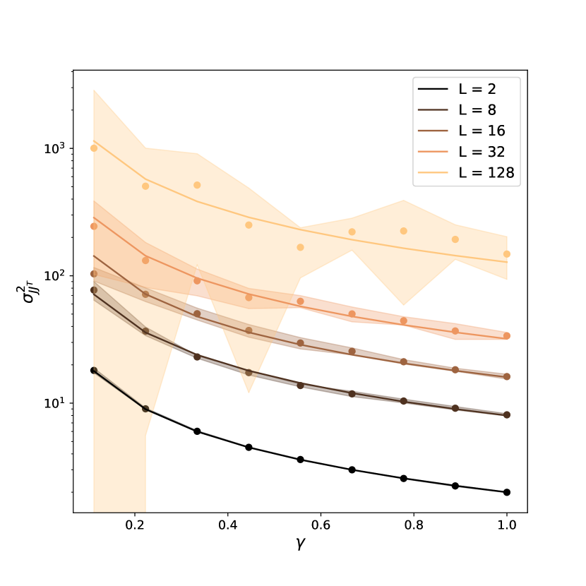
Figure 2: Evolution of the variance of the spectrum of $JJ^{T}$ with respect to $\gamma$ where $\gamma$ is the proportionality coefficient giving the rank of the weights matrices at layer $l$, whose width is $N_{l}$, $r_{l}=\gamma N_{l}$. Points are obtained empirically and averaged over 5 simulations when the lines are derived from the theory, see (11). Confidence intervals of 1 standard deviation around each mean point are shown. The weights are chosen to be low-rank Scaled Gaussian and the activation function is linear $\phi:x\mapsto x$. The same seed is used to initialise the weight matrices for each simulation and $q^{*}$ is set to 0.5. The $y-$axis is shown in log scale.

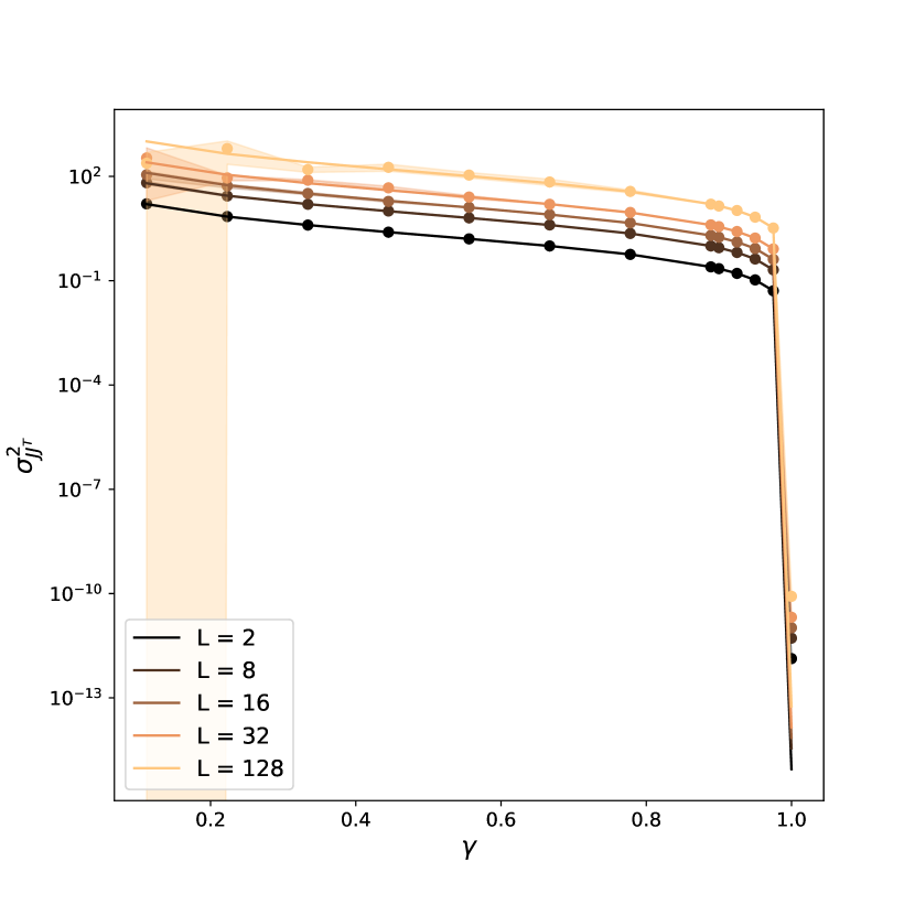
Figure 3: Evolution of the variance of the spectrum of $JJ^{T}$ with respect to $\gamma$ where $\gamma$ is the proportionality coefficient giving the rank of the weights matrices at layer $l$, whose width is $N_{l}$, $r_{l}=\gamma N_{l}$. Points are obtained empirically and averaged over 3 simulations when the lines are derived from the theory, see (11). Confidence intervals of 1 standard deviation around each mean point are shown. The weights are chosen to be low-rank Scaled Orthogonal and the activation function is linear $\phi:x\mapsto x$. The same seed is used to initialise the weight matrices for each simulation and $q^{*}$ is set to 0.5. The $y-$axis is shown in log scale.

Figure 4: Singular values of the Jacobian $J$ with respect to the depth of the network, whose weight matrices are low-rank Scaled Gaussian. The rank to width ratio $\gamma$ increases on each plot from left to right when the width is kept constant to $1000$. The activation function is erf. The same seed is used to initialise the weight matrices for each simulation and $q^{*}$ is set to 0.5. The $y-$axis is shown in log scale.

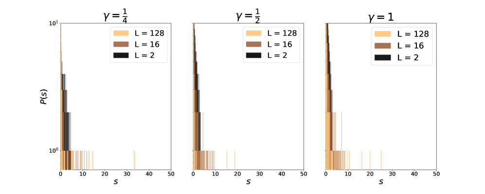
Figure 5: Singular values of the Jacobian $J$ with respect to the depth of the network, whose weight matrices are low-rank Scaled Gaussian. The rank to width ratio $\gamma$ increases on each plot from left to right when the width is kept constant to $1000$. The activation function is tanh. The same seed is used to initialise the weight matrices for each simulation and $q^{*}$ is set to 0.5. The $y-$axis is shown in log scale.

5 Summary and further work

Herein the edge-of-chaos theory of (Poole et al., 2016) and (Schoenholz et al., 2016) has been extended from the setting of full-rank weight matrices to the low-rank setting. Suitable scaling by the ratio of the rank to width factor $\gamma_{l}:=r_{l}/N_{l}$ recovers the phenomenon driven by the mean of the Jacobian’s spectra which defines the edge-of-chaos. Moreover, the variance of the Jacobian’s spectra is shown to be strictly increasing with decreasing $\gamma_{l}$ which suggests greater variability in the initial training of low-rank feedforward networks.

The edge-of-chaos initialisation scheme has been successfully generalised to a large set of different settings, including changes of architectures as CNNs (Xiao et al., 2018), LSTMs and GRUs (Gilboa et al., 2019), RNNs (Chen et al., 2018), ResNets (Yang & Schoenholz, 2017) and to extra features like dropout (Schoenholz et al., 2016), (Huang et al., 2019) or batch normalisation (Yang et al., 2019) and pruning (Hayou et al., 2020). It has been improved with changes of activation functions (Hayou et al., 2019), (Murray et al., 2021) to enable the data to propagate even deeper through the network. As a future work, each of these settings could be extended to the setting of low-rank weight matrices.

Appendix A Supplementary Material

A.1 Preliminary lemma

The following lemma is used later in the proofs contained in Section A.2.

Lemma A.1.

Let $\gamma\in\mathbb{R}^{*}$. If $C_{1},\dots,C_{\gamma n}\overset{\text{iid}}{\sim}\mathcal{N}(0,\frac{1}{n})$, then $C_{1}^{2}+\dots+C_{\gamma n}^{2}\to\gamma$ in probability when $n\to\infty$.

Proof. If $X$ is a random variable, let us denote by $F_{X}$ its cumulative distribution function. Let $x\in\mathbb{R}$.

$$F_{C_{1}^{2}+\dots+C_{\gamma n}^{2}}(x) =\mathbb{P}(C_{1}^{2}+\dots+C_{\gamma n}^{2}\leq x)$$

$$=\mathbb{P}(\sqrt{n}\frac{C_{1}^{2}+\dots+C_{\gamma n}^{2}-\gamma}{\sqrt{2\gamma}}\leq\sqrt{n}\frac{x-\gamma}{\sqrt{2\gamma}})$$

$$=\mathbb{P}(\frac{C_{1}^{2}+\dots+C_{\gamma n}^{2}-(n\gamma)\frac{1}{n}}{\frac{\sqrt{2}}{n}\sqrt{\gamma n}}\leq\sqrt{n}\frac{x-\gamma}{\sqrt{2\gamma}}).$$

where $$\mathbb{E}(C_{1}^{2})=\frac{1}{n} \mathbb{V}(C_{1}^{2})=\frac{\sqrt{2}}{n} n\to\infty \text{sign}(x-\gamma)\infty$$ and . Thus the Central Limit theorem holds and gives that the left hand side converges in distribution to a standard normal Gaussian when . The right hand side tends to . Thus

$$F_{C_{1}^{2}+\dots+C_{\gamma n}^{2}}(x) \to\mathds{1}_{x\geq\gamma}(x).$$

As we have a convergence in distribution towards a constant, the convergence in probability follows.

A.2 Distribution of hidden layers

Let us now consider at layer $l$ the weight matrix, $W^{(l)}\in\mathbb{R}^{N_{l}\times N_{l-1}}$, being of rank $r_{l}$:

$$W^{(l)}=\left[\begin{array}[]{c|c|c|c}&&&\\ \alpha^{(l)}_{1,1}C^{(l)}_{1}+\dots+\alpha^{(l)}_{r_{l},1}C^{(l)}_{r_{l}}&\alpha^{(l)}_{1,2}C^{(l)}_{1}+\dots+\alpha^{(l)}_{r_{l},2}C^{(l)}_{r_{l}}&\dots&\alpha^{(l)}_{1,N_{l-1}}C^{(l)}_{1}+\alpha^{(l)}_{r_{l},N_{l-1}}C^{(l)}_{r_{l}}\\ &&&\end{array}\right],$$

where, at any layer $l$, for any $k\in\llbracket 1,r_{l}\rrbracket$, the scalars $\left(\alpha^{(l)}_{k,i}\right)_{1\leq i\leq N_{l-1}}\in\mathbb{R}$ are identically and independently drawn from a Gaussian distribution $\mathcal{N}(0,\frac{\sigma_{\alpha}^{2}}{N_{l-1}})$ and the columns $C^{(l)}_{1},\dots,C^{(l)}_{r_{l}}$ are drawn jointly as the matrix $C^{(l)}:=[C^{(l)}_{1},\dots,C^{(l)}_{r_{l}}]\in\mathbb{R}^{N_{l}\times r_{l}}$ from the Grassmannian of rank $r$ matrices with orthonormal columns having zero mean and variance $1/N_{l}$. Similarly, in this section, we consider a random bias at layer $l$ along the directions given by $C^{(l)}_{1},\dots,C^{(l)}_{r_{l}}$, i.e. a bias of the form $b^{(l)}(C^{(l)}_{1}+\dots+C^{(l)}_{r_{l}})$, where $b^{(l)}\in\mathbb{R}\sim\mathcal{N}(0,\sigma_{b}^{2})$.

Thus, at layer $l$, whose width is $N_{l}$, the preactivation vector $h^{(l)}\in\mathbb{R}^{N_{l}}$ is given by

$$h^{(l)} =W^{(l)}\phi(h^{(l-1)})+b^{(l)}(C_{1}^{(l)}+\dots+C_{r_{l}}^{(l)})$$

$$=C_{1}^{(l)}\bigg{(}\underbrace{\sum\limits_{j=1}^{N_{l-1}}\alpha_{1,j}^{(l)}\phi(h^{(l-1)}_{j})+b^{(l)}}_{:=z_{1}^{(l)}}\bigg{)}+C_{2}^{(l)}\bigg{(}\underbrace{\sum\limits_{j=1}^{N_{l-1}}\alpha_{2,j}^{(l)}\phi(h^{(l-1)}_{j})+b^{(l)}}_{:=z_{2}^{(l)}}\bigg{)}+\dots+C_{r_{l}}^{l}\bigg{(}\underbrace{\sum\limits_{j=1}^{N_{l-1}}\alpha_{r_{l},j}^{(l)}\phi(h^{(l-1)}_{j})+b^{(l)}}_{:=z_{r_{l}}^{(l)}}\bigg{)}$$

$$=\sum\limits_{k=1}^{r_{l}}\underbrace{z_{k}^{(l)}}_{\in\mathbb{R}}C_{k}^{(l)},$$

where the scalars $z_{k}^{(l)}$ follow a Gaussian distribution, given the preactivation vector at the previous layer $z_{k}^{(l)}|_{h^{(l-1)}}\sim\mathcal{N}\bigg{(}0,\frac{\sigma^{2}_{\alpha}}{N_{l-1}}\sum\limits_{j=1}^{N_{l-1}}\phi(h^{(l-1)}_{j})^{2}+\sigma_{b}^{2}\bigg{)}$, which is given using the Central Limit Theorem in the large width $N_{l-1}$ regime.

A.3 Length recursion formula

This being said, one can compute the length of the (random) preactivation vector, at layer $l$.

$$q^{l} :=\frac{1}{N_{l}}||h^{(l)}||^{2}_{2}=\frac{1}{N_{l}}\sum\limits_{j=1}^{N_{l}}(h_{j}^{(l)})^{2}$$

$$=\frac{1}{N_{l}}\left((z_{1}^{(l)})^{2}||C^{(l)}_{1}||_{2}^{2}+\dots+(z_{r_{l}}^{(l)})^{2}||C^{(l)}_{r_{l}}||_{2}^{2}\right)\quad\text{ using Pythagore's theorem}$$

$$=\frac{1}{N_{l}}\left((z_{1}^{(l)})^{2}+\dots(z_{r_{l}}^{(l)})^{2}\right)\quad\text{ since for any $k$, }||C^{(l)}_{k}||_{2}=1$$

$$=\frac{1}{N_{l}}\sum\limits_{k=1}^{r_{l}}(z_{k}^{(l)})^{2}$$

Therefore, given $h^{(l-1)}$, $q^{l}$ is a sum of $r_{l}$ $\chi^{2}$ distributions.

Let us now consider at any layer, a rank that is proportional to the width: $r_{l}=\gamma_{l}N_{l}$, where $\gamma_{l}\in(0,1]$. Thus,

$$q^{l}=\gamma_{l}\frac{1}{\gamma_{l}N_{l}}\sum\limits_{k=1}^{\gamma_{l}N_{l}}(z_{k}^{(l)})^{2}.$$ (12)

Then all $z_{k}^{(l)}$ are independent and identically distributed Gaussian variables. The Law of Large Numbers holds and $q^{l}\to\gamma_{l}\mathbb{V}\big{(}z_{1}^{(l)}\big{)}$ when $N_{l}\to\infty$, with

$$\mathbb{V}\big{(}z_{1}^{(l)}\big{)}=\frac{\sigma^{2}_{\alpha}}{N_{l-1}}\sum\limits_{j=1}^{N_{l-1}}\phi(h^{(l-1)}_{j})^{2}+\sigma^{2}_{b}.$$

On the other hand,

$$h^{(l-1)}_{j}=\sum\limits_{k=1}^{r_{N_{l-1}}}z^{(l-1)}_{k}\big{(}C^{(l-1)}_{k}\big{)}_{j}=\big{(}z^{(l-1)}\big{)}^{T}\big{(}C^{(l-1)}_{.}\big{)}_{j}$$

denoting

$$\big{(}C^{(l)}_{.}\big{)}_{j}:=\begin{pmatrix}\big{(}C^{(l)}_{1}\big{)}_{j}\\ \vdots\\ \big{(}C^{(l)}_{r_{l}}\big{)}_{j}\end{pmatrix}$$

We know the distribution of $z^{(l-1)}\sim\mathcal{N}\bigg{(}\mathbb{O}_{\mathbb{R}^{r_{l-1}}},\frac{q^{l-1}}{\gamma_{l-1}}\mathbb{I}_{r_{l-1}}\bigg{)}$ and so, given $C^{(l-1)}$, $h^{(l-1)}_{j}\sim\mathcal{N}\bigg{(}0,\big{(}C^{(l-1)}_{.}\big{)}^{T}_{j}\frac{q^{l-1}}{\gamma_{l-1}}\mathbb{I}_{r_{l-1}}\big{(}C^{(l-1)}_{.}\big{)}_{j}\bigg{)}$.

In the asymptotic limit approximation, when $N_{l-1}\to\infty$, then $\big{(}C^{(l-1)}_{.}\big{)}^{T}_{j}\big{(}C^{(l-1)}_{.}\big{)}_{j}\to\gamma_{l-1}$ in probability as shown in Lemma A.1. Therefore, $h^{(l-1)}_{j}\sim\mathcal{N}\big{(}0,q^{l-1}\big{)}$.

In the limit when $N_{l-1}\to\infty$, the Law of Large Numbers enables us to conclude,

$$q^{l} =\gamma_{l}\big{(}\frac{\sigma^{2}_{\alpha}}{N_{l-1}}\sum\limits_{j=1}^{N_{l-1}}\phi(h^{(l-1)}_{j})^{2}+\sigma^{2}_{b}\big{)}$$

$$\to\gamma_{l} \big{(}\sigma^{2}_{\alpha}\int_{\mathbb{R}}\phi^{2}(\sqrt{q^{l-1}}z)Dz+\sigma_{b}^{2}\big{)}:=\mathcal{V}(q^{(l-1)}|\sigma^{2}_{\alpha},\sigma^{2}_{b},\gamma_{l}).$$

Note that when $\forall l,\gamma_{l}=1$ and $\sigma_{\alpha}=\sigma_{W}$, one recovers the formula from (Poole et al., 2016). Alternatively, by rescaling the variances by $\gamma_{l}$ at every layer, e.g. $\sigma^{2}_{\alpha}\to\frac{\sigma^{2}_{W}}{\gamma_{l}}$ and $\sigma_{b}^{2}\to\frac{\sigma^{2}_{b}}{\gamma_{l}}$, we recover the formulae of (Poole et al., 2016).

A.4 Correlation recursion formula

Let us denote by $x^{0,1}$ and $x^{0,2}$ two input data. Then one can define the following 2 by 2 matrix

$$(q^{l}_{ab})_{1\leq a,b\leq 2}=\frac{1}{N_{l}}\sum\limits_{i=1}^{N_{l}}\begin{pmatrix}h_{i}^{(l)}(x^{0,1})^{2}&h_{i}^{(l)}(x^{0,1})h_{i}^{(l)}(x^{0,2})\\ h_{i}^{(l)}(x^{0,1})h_{i}^{(l)}(x^{0,2})&h_{i}^{(l)}(x^{0,2})^{2}\end{pmatrix}$$

where, for $i\in\llbracket 1,N_{l}\rrbracket$, $h_{i}^{(l)}(x^{0,a})=\sum\limits_{r=1}^{r_{l}}z_{k}^{(l)}(x^{0,a})\big{(}C^{(l)}_{k}\big{)}_{i}$.

So,

$$\frac{1}{N_{l}}\sum\limits_{i=1}^{N_{l}}h_{i}^{(l)}(x^{0,1})h_{i}^{(l)}(x^{0,2}) =\frac{1}{N_{l}}\sum\limits_{i=1}^{N_{l}}\bigg{(}\sum\limits_{k=1}^{r_{l}}z_{k}^{(l)}(x^{0,1})\big{(}C^{(l)}_{k}\big{)}_{i}\bigg{)}\bigg{(}\sum\limits_{p=1}^{r_{l}}z_{p}^{(l)}(x^{0,2})\big{(}C^{(l)}_{p}\big{)}_{i}\bigg{)}$$

$$=\frac{1}{N_{l}}\sum\limits_{k=1}^{r_{l}}z_{k}^{(l)}(x^{0,1})z_{k}^{(l)}(x^{0,2})\bigg{(}\underbrace{\sum\limits_{i=1}^{N_{l}}\big{(}C^{(l)}_{k}\big{)}_{i}^{2}}_{||C^{(l)}_{k}||_{2}^{2}=1}\bigg{)}+\frac{1}{N_{l}}\sum\limits_{\begin{subarray}{c}1\leq k,p\leq r_{l}\\ k\neq p\end{subarray}}z_{k}^{(l)}(x^{0,1})z_{p}^{(l)}(x^{0,2})\bigg{(}\underbrace{\sum\limits_{i=1}^{N_{l}}\big{(}C^{(l)}_{k}\big{)}_{i}\big{(}C^{(l)}_{p}\big{)}_{i}}_{\langle C^{(l)}_{k},C^{(l)}_{p}\rangle=0}\bigg{)}$$

$$=\frac{1}{N_{l}}\sum\limits_{k=1}^{r_{l}}z_{k}^{(l)}(x^{0,1})z_{k}^{(l)}(x^{0,2})$$

Therefore, when the rank is proportional to the width and the width $$N_{l}\to\infty$$ as previously, the Law of Large Numbers gives

$$=\gamma_{l}\frac{1}{\gamma_{l}N_{l}}\sum\limits_{k=1}^{r_{l}}z_{k}^{(l)}(x^{0,1})z_{k}^{(l)}(x^{0,2})\to\gamma_{l}Cov\bigg{(}z_{1}^{(l)}(x^{0,2}),z_{1}^{(l)}(x^{0,2})\bigg{)}$$

On the other hand,

$$Cov\bigg{(}z_{1}^{(l)}(x^{0,1}),z_{1}^{(l)}(x^{0,2})\bigg{)} =\sum\limits_{1\leq i,j\leq N_{l-1}}\phi(h^{(l-1)}_{i}(x^{0,1}))\phi(h^{(l-1)}_{j}(x^{0,2}))\underbrace{Cov(\alpha^{(l)}_{1,i},\alpha^{(l)}_{1,j})}_{\frac{\sigma_{\alpha}}{N_{l-1}}\delta_{i,j}}$$

$$+\sum\limits_{1\leq i\leq N_{l-1}}\phi(h^{(l-1)}_{i}(x^{0,1}))\underbrace{Cov(\alpha^{(l)}_{1,i},b^{(l)}_{1})}_{=0}$$

$$+\sum\limits_{1\leq i\leq N_{l-1}}\phi(h^{(l-1)}_{i}(x^{0,2}))\underbrace{Cov(\alpha^{(l)}_{1,i},b^{(l)}_{1})}_{=0}+\underbrace{Cov(b^{(l)}_{1},b^{(l)}_{1})}_{\sigma_{b}^{2}}$$

Thus, when $N_{l-1}\to\infty$, the Law of Large Numbers enables us to conclude

$$q^{l}_{12}=\gamma_{l}\bigg{(}\sigma^{2}_{\alpha}\int_{\mathbb{R}^{2}}\phi(\sqrt{q^{l-1}_{11}}z_{1})\phi(\sqrt{q^{l-1}_{22}}(c_{12}^{l-1}z_{1}+\sqrt{1-(c_{12}^{l-1})^{2}}z_{2})Dz_{1}Dz_{2}+\sigma^{2}_{b}\bigg{)}$$

with $$c_{12}^{l}=q_{12}^{l}(q_{11}^{l}q_{22}^{l})^{-\frac{1}{2}}$$.

Note that if we consider the short convergence of the variance, compared to the covariance one, as observed in (Poole et al., 2016), then we can assume $q_{11}^{l}\approx q_{22}^{l}\approx q^{*}$. We can then rescale the previous covariance map to get the correlation map as follows:

$$c^{l}_{12}=\frac{\gamma_{l}}{q^{*}}\bigg{(}\sigma^{2}_{\alpha}\int_{\mathbb{R}^{2}}\phi(\sqrt{q^{*}}z_{1})\phi(\sqrt{q^{*}}(c_{12}^{l-1}z_{1}+\sqrt{1-(c_{12}^{l-1})^{2}}z_{2})Dz_{1}Dz_{2}+\sigma^{2}_{b}\bigg{)}$$

We observe that $1$ is always a fixed point as $1=\frac{\gamma_{l}}{q^{*}}\bigg{(}\sigma^{2}_{\alpha}\int_{\mathbb{R}}Dz\phi^{2}(\sqrt{q^{*}}z)+\sigma_{b}^{2}\bigg{)}=\frac{1}{q^{*}}\mathcal{V}(q^{*}|\sigma_{\alpha}^{2},\sigma_{b}^{2},\gamma)=\frac{q^{*}}{q^{*}}$.

For completeness we replicate correlation maps and dynamics of correlations through layers using the same parameters as in (Poole et al., 2016) suitably modified for the low-rank setting, see Figure 6 - 9. The dynamics of the low-rank networks are observed to be consistent, under appropriate scaling by $\gamma_{l}$,with those of the full-rank networks in (Poole et al., 2016).

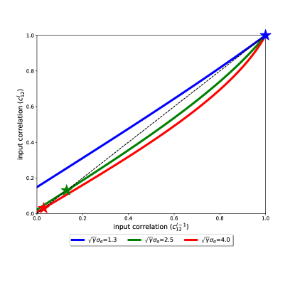
Figure 6: Correlation map of a low-rank neural network where the rank is proportional to the width by a factor $\gamma$. The nonlinear activation function is $\phi=\text{tanh}$. The map is given by (6) and the integral is computed numerically. The dashed line is the identity function and stars represent fixed points of the correlation map.

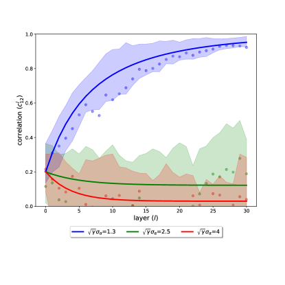
Figure 7: Dynamic of the correlation through layers, starting from two input vectors with correlation $c^{0}_{12}=0.2$. Points are obtained empirically and averaged over 5 simulations when the lines are derived from the theory, see (6). Confidence intervals of 2 standard deviations around each point are shown. For each point on the plot, we generated a pair of points with correlation $c^{0}_{12}$, passed them through a Wide low-rank network initialised and computed the correlation between both preactivation vectors across layers. The network has constant width $N=1000$. $\sigma_{b}=0.3,\phi=\text{tanh},\gamma=\frac{1}{4}$.

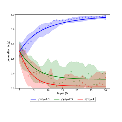
Figure 8: Dynamic of the correlation through layers, starting from two input vectors with correlation $c^{0}_{12}=0.5.$. Points are obtained empirically and averaged over 5 simulations when the lines are derived from the theory, see (6). Confidence intervals of 2 standard deviations around each point are shown. For each point on the plot, we generated a pair of points with correlation $c^{0}_{12}$, passed them through a Wide low-rank network initialised and computed the correlation between both preactivation vectors across layers. The network has constant width $N=1000$. $\sigma_{b}=0.3,\phi=\text{tanh},\gamma=\frac{1}{4}$.

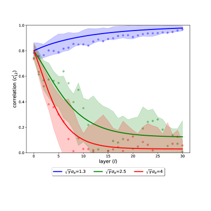
Figure 9: Dynamic of the correlation through layers, starting from two input vectors with correlation $c^{0}_{12}=0.8.$. Points are obtained empirically and averaged over 5 simulations when the lines are derived from the theory, see (6). Confidence intervals of 2 standard deviations around each point are shown. For each point on the plot, we generated a pair of points with correlation $c^{0}_{12}$, passed them through a Wide low-rank network initialised and computed the correlation between both preactivation vectors across layers. The network has constant width $N=1000$. $\sigma_{b}=0.3,\phi=\text{tanh},\gamma=\frac{1}{4}$.

A.5 Derivative of the correlation map

In this section, we extend the computations of the derivative of the correlation map.

$$\frac{\partial c^{l}_{12}}{\partial c^{l-1}_{12}} =\frac{\gamma_{l}}{q^{*}}\bigg{(}\sigma^{2}_{\alpha}\int_{\mathbb{R}^{2}}\phi(u_{1})\phi^{\prime}(u_{2})\big{(}\sqrt{q^{*}}z_{1}-\sqrt{q^{*}}\frac{c^{l-1}_{12}}{\sqrt{1-(c^{l-1}_{12})^{2}}}z_{2}\big{)}Dz_{1}Dz_{2}\bigg{)}$$

Using, for $$F \int_{\mathbb{R}}F(z)zDz=\int_{\mathbb{R}}F^{\prime}(z)Dz G:z_{1}\mapsto\phi(\sqrt{q^{*}}z_{1})\int_{z_{2}}\phi^{\prime}\big{(}\sqrt{q^{*}}(c^{l-1}_{12}z_{1}+\sqrt{1-(c^{l-1}_{12})^{2}}z_{2})\big{)}Dz_{2} H:z_{2}\mapsto\int_{z_{1}}\phi(\sqrt{q^{*}}z_{1})\phi^{\prime}\big{(}\sqrt{q^{*}}(c^{l-1}_{12}z_{1}+\sqrt{1-(c^{l-1}_{12})^{2}}z_{2})\big{)}Dz_{1}$$ smooth enough, the identity to the functions and , we obtain

$$\frac{\partial c^{l}_{12}}{\partial c^{l-1}_{12}} =\gamma_{l}\sigma^{2}_{\alpha}\int_{\mathbb{R}^{2}}\phi^{\prime}(\sqrt{q^{*}}z_{1})\phi^{\prime}\big{(}\sqrt{q^{*}}(c_{12}^{l-1}z_{1}+\sqrt{1-(c_{12}^{l-1})^{2}}z_{2})\big{)}Dz_{1}Dz_{2},$$

which, evaluated at its fixed point $$c^{l-1}_{12}=1$$ gives

$$\chi_{\gamma} :=\frac{\partial c^{l}_{12}}{\partial c^{l-1}_{12}}|_{c^{l-1}_{12}=1}=\gamma_{l}\sigma^{2}_{\alpha}\int_{\mathbb{R}}\bigg{(}\phi^{\prime}(\sqrt{q^{*}}z)\bigg{)}^{2}Dz.$$

The edge-of-chaos level set defined by $\chi_{\gamma}=1$ for nonlinear activation $\phi(x)=tanh(x)$ is shown in Figure 1 with axes $\gamma\sigma_{w}^{2}$ and $\gamma\sigma_{b}^{2}$. Figure 10 show the analogous edge-of-chaos plot for a full-rank matrix as given, which is identical to that of 1 but with axes $\sigma_{w}^{2}$ and $\sigma_{b}^{2}$.

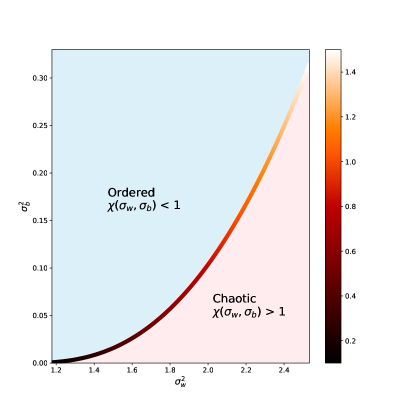
Figure 10: Original edge-of-chaos curve of the full-rank feedforward neural network with nonlinear activation $\phi(x)=tanh(x)$.

A.6 Length depth scale

Recall that $q^{l}=\gamma_{l}\big{(}\sigma_{\alpha}^{2}\int Dz\phi^{2}(\sqrt{q^{l-1}}z)+\sigma_{b}^{2}\big{)}$ and $q^{*}$ is a fixed point assumed to exist when $\gamma_{l}=\gamma$ at any layer $l$. We then define the perturbation $\epsilon_{l}\to 0$ such that $q^{l}=q^{*}+\epsilon_{l}$. We can then expand the relation around its fixed point, as done in the case of feedforward neural network in (Schoenholz et al., 2016).

$$q^{l+1} =q^{*}+\epsilon_{l+1}=\gamma\big{(}\sigma_{\alpha}^{2}\int Dz\phi^{2}((\epsilon_{l}+q^{*})^{\frac{1}{2}}z)+\sigma_{b}^{2}\big{)}$$

$$=\gamma\bigg{(}\sigma_{\alpha}^{2}\int Dz\phi\big{(}\sqrt{q^{*}}z+\frac{1}{2}\frac{\epsilon_{l}}{\sqrt{q^{*}}}z+\mathcal{O}(\epsilon_{l}^{2})\big{)}^{2}+\sigma_{b}^{2}\bigg{)}\text{ expanding the square root}$$

$$=\gamma\bigg{(}\sigma_{\alpha}^{2}\int Dz\big{(}(\phi(\sqrt{q^{*}}z)+\phi^{\prime}(\sqrt{q^{*}}z)\frac{\epsilon_{l}}{2\sqrt{q^{*}}}z+\mathcal{O}(\epsilon_{l}^{2})\big{)}^{2}+\sigma_{b}^{2}\bigg{)}\text{ expanding $\phi$ around $\sqrt{q^{*}}z$}$$

$$=\gamma\bigg{(}\sigma_{\alpha}^{2}\int Dz\phi^{2}(\sqrt{q^{*}}z)+\int Dz\phi^{\prime}(\sqrt{q^{*}}z)\phi(\sqrt{q^{*}}z)\frac{\epsilon_{l}}{\sqrt{q^{*}}}z+\mathcal{O}(\epsilon_{l}^{2})+\sigma_{b}^{2}\bigg{)}$$

$$=q^{*}+\gamma\int Dz\phi^{\prime}(\sqrt{q^{*}}z)\phi(\sqrt{q^{*}}z)\frac{\epsilon_{l}}{\sqrt{q^{*}}}z+\mathcal{O}(\epsilon_{l}^{2})\text{ by definition of $q^{*}$}$$

$$=q^{*}+\epsilon_{l}\gamma\sigma_{\alpha}^{2}\bigg{(}\int Dz\big{(}\phi^{\prime}(\sqrt{q^{*}}z)\big{)}^{2}+\int Dz\phi^{\prime\prime}(\sqrt{q^{*}}z)\phi(\sqrt{q^{*}}z)\bigg{)}+\mathcal{O}(\epsilon_{l}^{2})\text{ using $\int DzF(z)z=\int DzF^{\prime}(z)$}$$

Note that in the proof above we assumed the activation function $\phi$ to be smooth enough to use its Taylor expansion around the point $\sqrt{q^{*}}z$ for any $z$.

Therefore by identification, $\epsilon_{l+1}=\epsilon_{l}\big{(}\chi_{\gamma}+\gamma\sigma^{2}_{\alpha}\int Dz\phi^{\prime\prime}(\sqrt{q^{*}}z)\phi(\sqrt{q^{*}}z)\big{)}+\mathcal{O}(\epsilon_{l}^{2})$, which concludes the proof.

A.7 Correlation depth scale

Let consider the computation is done at a layer $l$ deep enough so that the variance map has already converged towards its fixed point $q^{l}_{11}=q^{l}_{22}=q^{*}$. We generate a perturbation $\epsilon_{l}\underset{l\to\infty}{\to}0$ around the fixed point $c^{*}$ and analyse how it propagates: $c^{l}_{12}=c^{*}+\epsilon_{l}$. Additionally, we introduce $u_{1}^{l}=\sqrt{q^{*}}z=u_{1}^{*},u_{2}^{*}=\sqrt{q^{*}}(c^{*}z_{1}+\sqrt{1-(c^{*})^{2}}z_{2})$ and $u_{2}^{l}=\sqrt{q^{*}}(c^{l}_{12}z_{1}+\sqrt{1-(c^{l}_{12})^{2}}z_{2})$. Following the same strategy as in the previous section (using expansions), it is shown in (Schoenholz et al., 2016) that

$$u_{2}^{l}=\begin{cases}u_{2}^{*}+\sqrt{q^{*}}\epsilon_{l}\big{(}z_{1}-\frac{c^{*}}{\sqrt{1-{c^{*}}^{2}}}z_{2}\big{)}+\mathcal{O}(\epsilon_{l}^{2})&\text{ when $c^{*}<1$,}\\ u_{2}^{*}+\sqrt{2q^{*}\epsilon_{l}}z_{2}-\epsilon_{l}\sqrt{q^{*}}z_{1}+\mathcal{O}(\epsilon_{l}^{\frac{3}{2}})&\text{ when $c^{*}=1$}.\end{cases}$$

Therefore, in the first case $c^{*}<1$,

$$c^{l+1}_{12} =c^{*}+\epsilon_{l}=\frac{\gamma_{l}}{q^{*}}\bigg{(}\sigma^{2}_{\alpha}\int_{\mathbb{R}^{2}}Dz_{1}Dz_{2}\phi(u^{*}_{1})\phi(u_{2}^{l})+\sigma^{2}_{b}\bigg{)}$$

$$=\frac{\gamma_{l}}{q^{*}}\bigg{(}\sigma^{2}_{\alpha}\int_{\mathbb{R}^{2}}Dz_{1}Dz_{2}\phi(u^{*}_{1})\phi(u_{2}^{*}+\sqrt{q^{*}}\epsilon_{l}\big{(}z_{1}-\frac{c^{*}}{\sqrt{1-{c^{*}}^{2}}}z_{2}\big{)}+\mathcal{O}(\epsilon_{l}^{2}))+\sigma^{2}_{b}\bigg{)}$$

$$=\frac{\gamma_{l}}{q^{*}}\bigg{(}\sigma^{2}_{\alpha}\int_{\mathbb{R}^{2}}Dz_{1}Dz_{2}\phi(u^{*}_{1})[\phi(u_{2}^{*})+\phi^{\prime}(u_{2}^{*})\sqrt{q^{*}}\epsilon_{l}\big{(}z_{1}-\frac{c^{*}}{\sqrt{1-{c^{*}}^{2}}}z_{2}\big{)}]+\mathcal{O}(\epsilon_{l}^{2})+\sigma^{2}_{b}\bigg{)}\text{ expanding $\phi$ around $u_{2}^{*}$}$$

$$=c^{*}+\frac{\gamma_{l}}{\sqrt{q^{*}}}\sigma_{\alpha}^{2}\epsilon_{l}\int_{\mathbb{R}^{2}}Dz_{1}Dz_{2}\phi(u^{*}_{1})\phi^{\prime}(u_{2}^{*})z_{1}-\frac{c^{*}}{\sqrt{1-{c^{*}}^{2}}}\frac{\gamma_{l}}{\sqrt{q^{*}}}\int_{\mathbb{R}^{2}}Dz_{1}Dz_{2}\phi(u^{*}_{1})\phi^{\prime}(u_{2}^{*})z_{2}+\mathcal{O}(\epsilon_{l}^{2})$$

$$=c^{*}+\gamma_{l}\sigma_{\alpha}^{2}\epsilon_{l}\int_{\mathbb{R}^{2}}Dz_{1}Dz_{2}\phi(u^{*}_{1})\big{(}\phi^{\prime}(u_{2}^{*})+c^{*}\phi^{\prime\prime}(u_{2}^{*})\big{)}-c^{*}\gamma_{l}\int_{\mathbb{R}^{2}}Dz_{1}Dz_{2}\phi(u^{*}_{1})\phi^{\prime}\prime(u_{2}^{*})+\mathcal{O}(\epsilon_{l}^{2})$$

$$=c^{*}+\gamma_{l}\sigma_{\alpha}^{2}\epsilon_{l}\int_{\mathbb{R}^{2}}Dz_{1}Dz_{2}\phi(u^{*}_{1})\phi^{\prime}(u_{2}^{*})+\mathcal{O}(\epsilon_{l}^{2})$$

where the second to last line is obtained using $\int DzF(z)z=\int DzF^{\prime}(z)$, for $\phi$ smooth enough. We can then identify $\epsilon_{l+1}=\epsilon_{l}\gamma_{l}\sigma_{\alpha}^{2}\int_{\mathbb{R}^{2}}Dz_{1}Dz_{2}\phi(u^{*}_{1})\phi^{\prime}(u_{2}^{*})+\mathcal{O}(\epsilon_{l}^{2})$.

In the second case $c^{*}=1$, $u_{1}^{*}=u_{2}^{*}$, $c^{l}_{12}=1-\epsilon_{l}$ and we expand $\phi$ around $u_{2}^{*}$ until to the second order.

$$c^{l+1}_{12} =1-\epsilon_{l+1}=\frac{\gamma_{l}}{q^{*}}\bigg{(}\sigma^{2}_{\alpha}\int_{\mathbb{R}^{2}}Dz_{1}Dz_{2}\phi(u^{*}_{1})\phi(u_{2}^{l})+\sigma^{2}_{b}\bigg{)}$$

$$=\frac{\gamma_{l}}{q^{*}}\bigg{(}\sigma^{2}_{\alpha}\int_{\mathbb{R}^{2}}Dz_{1}Dz_{2}\phi(u^{*}_{1})\phi\big{(}u_{2}^{*}+\sqrt{q^{*}}\epsilon_{l}\big{(}z_{1}-\frac{c^{*}}{\sqrt{1-{c^{*}}^{2}}}z_{2}\big{)}+\mathcal{O}(\epsilon_{l}^{2})\big{)}+\sigma^{2}_{b}\bigg{)}$$

$$=\frac{\gamma_{l}}{q^{*}}\bigg{(}\sigma^{2}_{\alpha}\int_{\mathbb{R}^{2}}Dz_{1}Dz_{2}\phi(u^{*}_{1})\bigg{(}\phi(u_{2}^{*})+\phi^{\prime}(u_{2}^{*})\big{(}\sqrt{2q^{*}\epsilon_{l}}z_{2}-\sqrt{q^{*}}\epsilon_{l}z_{1}\big{)}+\phi^{\prime\prime}(u_{2}^{*})\frac{1}{2}\big{(}\sqrt{2q^{*}\epsilon_{l}}z_{2}-\sqrt{q^{*}}\epsilon_{l}z_{1}\big{)}^{2}+\mathcal{O}(\epsilon_{l}^{\frac{3}{2}})\big{)}+\sigma^{2}_{b}\bigg{)}$$

$$=c^{*}+\frac{\gamma_{l}}{\sqrt{q^{*}}}\sqrt{2\epsilon_{l}}\sigma^{2}_{\alpha}\int_{\mathbb{R}}Dz_{1}\phi(u^{*}_{1})\phi^{\prime}(u_{2}^{*})\underbrace{\int_{\mathbb{R}}z_{2}Dz_{2}}_{=0}-\frac{\gamma_{l}}{\sqrt{q^{*}}}\epsilon_{l}\sigma^{2}_{\alpha}\int_{\mathbb{R}}Dz_{1}\phi(u^{*}_{1})\phi^{\prime}(u_{2}^{*})z_{1}\underbrace{\int_{\mathbb{R}}Dz_{2}}_{=1}$$

$$\qquad\qquad+\gamma_{l}\epsilon_{l}\sigma^{2}_{\alpha}\int_{\mathbb{R}}Dz_{1}\phi(u^{*}_{1})\phi^{\prime\prime}(u_{2}^{*})\underbrace{\int_{\mathbb{R}}z_{2}^{2}Dz_{2}}_{=1}+\mathcal{O}(\epsilon_{l}^{\frac{3}{2}})$$

$$=c^{*}-\frac{\gamma_{l}}{\sqrt{q^{*}}}\epsilon_{l}\sigma^{2}_{\alpha}\int_{\mathbb{R}}Dz_{1}\phi(u^{*}_{1})\phi^{\prime}(u_{2}^{*})z_{1}+\gamma_{l}\epsilon_{l}\sigma^{2}_{\alpha}\int_{\mathbb{R}}Dz_{1}\phi(u^{*}_{1})\phi^{\prime\prime}(u_{2}^{*})+\mathcal{O}(\epsilon_{l}^{\frac{3}{2}})$$

$$=c^{*}-\gamma_{l}\epsilon_{l}\sigma^{2}_{\alpha}\int_{\mathbb{R}}Dz_{1}(\phi^{\prime}(u_{1}^{*}))^{2}-\gamma_{l}\epsilon_{l}\sigma^{2}_{\alpha}\int_{\mathbb{R}}Dz_{1}\phi(u_{1}^{*})\phi^{\prime\prime}(u_{2}^{*})+\gamma_{l}\epsilon_{l}\sigma^{2}_{\alpha}\int_{\mathbb{R}}Dz_{1}\phi(u^{*}_{1})\phi^{\prime\prime}(u_{2}^{*})+\mathcal{O}(\epsilon_{l}^{\frac{3}{2}})$$

$$=c^{*}-\epsilon_{l}\gamma_{l}\sigma^{2}_{\alpha}\int_{\mathbb{R}}Dz(\phi^{\prime}(\sqrt{q^{*}}z))^{2}+\mathcal{O}(\epsilon_{l}^{\frac{3}{2}})$$

Therefore, $\epsilon_{l+1}=\epsilon_{l}\gamma_{l}\sigma^{2}_{\alpha}\int_{\mathbb{R}}Dz(\phi^{\prime}(\sqrt{q^{*}}z))^{2}+\mathcal{O}(\epsilon_{l}^{\frac{3}{2}})$, which concludes the proof.

Figure 11 shows the analytically calculated correlation depth scales as a function of $\gamma\sigma_{\alpha}^{2}$ as well as simulations with networks of width $N=1000$ and nonlinear activation $\phi(x)=tanh(x)$. The networks depth scale are observed to be consistent with the analytic calculations; in particular showing the depth scale asymptotes at $\chi_{\gamma}=1$ for the different choices of $\sigma_{b}^{2}$.

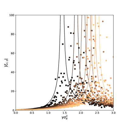
Figure 11: Correlation depth scale with respect to $\gamma\sigma^{2}_{\alpha}$ diverging when $\chi_{\gamma}=1$. Points are obtained empirically when the lines are derived from the theory. The variance of the bias varies from $\sigma^{2}_{b}=0.01\gamma^{-1}$ (black) to $\sigma^{2}_{b}=0.3\gamma^{-1}$ (yellow). The network has constant width $N=1000$. $\phi=\text{tanh},\gamma=\frac{1}{4}$.

A.8 Backpropagation

Recall that $h_{i}^{(l)}=\sum\limits_{k=1}^{r_{l}}\bigg{(}\sum\limits_{j=1}^{N_{l-1}}\alpha_{k,j}^{(l)}\phi(h^{(l-1)}_{j})+b^{(l)}\bigg{)}(C_{k}^{(l)})_{i}$. Then the chain rule immediately gives,

$$\delta_{j}^{l}:=\frac{\partial E}{\partial h_{j}^{(l)}}=\big{(}\sum_{k=1}^{N_{l+1}}\delta_{k}^{l+1}W_{kj}^{(l+1)}\big{)}\phi^{\prime}(h_{j}^{(l)})$$

Because the trainable parameters of our network are the coefficients $\alpha_{ij}^{(l)}$, we compute the gradient of the error loss $E$ with respect to them. So we need to adapt the proof from (Schoenholz et al., 2016), derived in the standard feedforward case as follows.

$$||\nabla_{\alpha_{ij}^{(l)}}E||^{2}_{2} =\sum_{i,j}\big{(}\frac{\partial E}{\partial\alpha_{ij}^{(l)}}\big{)}^{2}$$

$$\underset{N_{l},N_{l+1}\to\infty}{\approx}N_{l}N_{l+1}\mathbb{E}\bigg{(}\big{(}\frac{\partial E}{\partial\alpha_{ij}^{(l)}}\big{)}^{2}\bigg{)}.$$

Since, assuming all these partial derivatives to be identically and independently distributed, the Law of Large numbers holds.

On the one hand,

$$\frac{\partial E}{\partial\alpha^{(l)}} =\sum_{m=1}^{N_{l}}\frac{\partial E}{\partial h_{m}^{(l)}}\frac{\partial h_{m}^{(l)}}{\partial\alpha_{ij}^{(l)}}=\sum_{m=1}^{N_{l}}\delta_{m}^{l}\phi(h_{j}^{(l-1)})(C_{i}^{(l)})_{m}=\bigg{(}\sum_{m=1}^{N_{l}}\delta_{m}^{l}(C_{i}^{(l)})_{m}\bigg{)}\phi(h_{j}^{(l-1)}).$$

Therefore, assuming independence between the weights used for the forward pass and the weights backpropagated,

$$\mathbb{E}\bigg{(}\big{(}\frac{\partial E}{\partial\alpha_{ij}^{(l)}}\big{)}^{2}\bigg{)} =\mathbb{E}\bigg{(}\big{(}\sum_{m=1}^{N_{l}}\delta_{m}^{l}(C_{i}^{(l)})_{m}\big{)}^{2}\bigg{)}\mathbb{E}\big{(}\phi^{2}(h_{j}^{(l-1)})\big{)}$$

$$=\mathbb{E}\bigg{(}\sum_{m=1}^{N_{l}}(\delta_{m}^{l})^{2}(C_{i}^{(l)})_{m}^{2}+\sum_{p,m}\delta_{m}^{l}(C_{i}^{(l)})_{m}\bigg{)}\mathbb{E}\big{(}\phi^{2}(h_{j}^{(l-1)})\big{)}$$

$$=\frac{1}{N_{l}}\sum_{m=1}^{N_{l}}\mathbb{E}\big{(}(\delta_{m}^{l})^{2}\big{)}\mathbb{E}\big{(}\phi^{2}(h_{j}^{(l-1)})\big{)}\text{ since $(C_{1}^{(l)})_{m}\overset{\text{iid}}{\sim}\mathcal{N}(0,\frac{1}{N_{l}})$}$$

$$=\mathbb{E}\big{(}(\delta_{1}^{l})^{2}\big{)}\mathbb{E}\big{(}\phi^{2}(h_{j}^{(l-1)})\big{)}.$$

Therefore, the length of the gradient loss is proportional to the variance of $\delta_{1}^{l}$.

On the other hand, denoting with a subscript the function $f_{a}$ when fed with input data $x^{0,a}$,

$$\tilde{q}^{l}_{aa} :=\mathbb{E}\big{(}(\delta_{1,a}^{l})^{2}\big{)}$$

$$=\mathbb{E}\bigg{(}\big{(}\sum_{k=1}^{N_{l+1}}\delta_{k,a}^{l+1}W_{kj}^{(l+1)}\big{)}^{2}\bigg{)}\mathbb{E}\bigg{(}\big{(}\phi^{\prime}(h_{j,a}^{(l)})\big{)}^{2}\bigg{)}$$

$$=\bigg{(}\sum_{k=1}^{N_{l+1}}\mathbb{E}\big{(}(\delta_{k,a}^{l+1})^{2}\big{)}\mathbb{E}\big{(}(W_{kj}^{(l+1)})^{2}\big{)}\bigg{)}\mathbb{E}\bigg{(}\big{(}\phi^{\prime}(h_{j,a}^{(l)})\big{)}^{2}\bigg{)}$$

where we used again the assumed independence. The first and second order moments of $$W_{ij}^{(l)} \mathbb{E}(W_{ij}^{(l)})=0 \mathbb{E}\big{(}(W_{ij}^{(l)})^{2}\big{)}=\mathbb{E}\big{(}(\sum\limits_{p=1}^{r_{l}}\alpha_{p,j}^{(l)}(C_{p}^{(l)})_{i})^{2}\big{)}=\sum\limits_{p=1}^{r_{l}}\mathbb{V}(\alpha_{p,j}^{(l)})\mathbb{V}((C_{p}^{(l)})_{i})=r_{l}\frac{\sigma^{2}_{\alpha}}{N_{l-1}}\frac{1}{N_{l}}$$ are given by and . Thus,

$$\tilde{q}^{l}_{aa} =r_{l+1}\frac{\sigma^{2}_{\alpha}}{N_{l}}\frac{1}{N_{l+1}}\bigg{(}\sum_{k=1}^{N_{l+1}}\mathbb{E}\big{(}(\delta_{k,a}^{l+1})^{2}\big{)}\bigg{)}\mathbb{E}\bigg{(}\big{(}\phi^{\prime}(h_{j,a}^{(l)})\big{)}^{2}\bigg{)}$$

$$=r_{l+1}\frac{\sigma^{2}_{\alpha}}{N_{l}}\frac{1}{N_{l+1}}N_{l+1}\tilde{q}^{l+1}_{aa}\mathbb{E}\bigg{(}\big{(}\phi^{\prime}(h_{j,a}^{(l)})\big{)}^{2}\bigg{)}$$

$$=r_{l+1}\frac{\sigma^{2}_{\alpha}}{N_{l}}\frac{1}{N_{l+1}}N_{l+1}\tilde{q}^{l+1}_{aa}\int Dz\big{(}\phi^{\prime}(\sqrt{q_{aa}^{l-1}}z)\big{)}^{2}\text{ as $h_{j,a}^{(l-1)}\sim\mathcal{N}(0,q_{aa}^{l-1})$.}$$

Considering that the computation is done at a layer deep enough, since $$q^{l-1} q^{*} q_{aa}^{l-1}\approx q^{*} r_{l}=\gamma_{l}N_{l}$$ converges to shortly, then , and, as ,

$$\tilde{q}^{l}_{aa} =\tilde{q}^{l+1}_{aa}\gamma_{l+1}\sigma^{2}_{\alpha}\int Dz\big{(}\phi^{\prime}(\sqrt{q^{*}}z)\big{)}^{2}=\tilde{q}^{l+1}_{aa}\chi_{l+1}.$$

Figure 12 demonstrates the exponential evolution of $||\nabla_{\alpha^{(l)}}E||^{2}_{2}$ from the final layer, $L=250$, to the earlier layers. The analytic expressions are shown to be consistent with simulation from random low-rank networks with nonlinear activation $\phi(x)=tanh(x)$, rank to width scale $\gamma=1/4$, the bias variance $\sigma_{b}^{2}$ held fixed and $\sigma_{\alpha}^{2}$ varying.

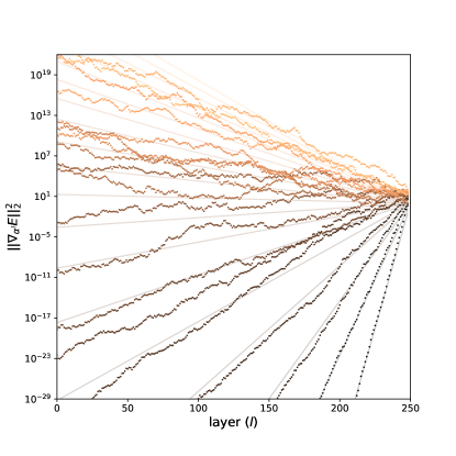
Figure 12: Exponential evolution of the propagation of the $L_{2}$-norm of the gradient with respect to the depth for a $250$ layer deep random neural network with a cross entropy loss on MNIST dataset. Points are obtained empirically when the lines are derived from the theory. The variance of the weights $\gamma\sigma^{2}_{\alpha}$ varies from $0.01\gamma^{-1}$ (black) to $0.3\gamma^{-1}$ (yellow) when the variance of the bias $\gamma\sigma_{b}^{2}$ is kept fixed to $0.05$. $\phi=\text{tanh},\gamma=\frac{1}{4}$.

A.9 Average singular value of $D^{l}W^{(l)}$

As a preliminary, let us first note that $\frac{1}{N_{l}}\text{Tr}\bigg{(}D^{l}W^{(l)}(D^{l}W^{(l)})^{T}\bigg{)}=\frac{1}{N_{l}}\sum\limits_{k=1}^{N_{l}}\lambda_{k}\bigg{(}D^{l}W^{(l)}(D^{l}W^{(l)})^{T}\bigg{)}=\frac{1}{N_{l}}\sum\limits_{k=1}^{N_{l}}\sigma^{2}_{k}\bigg{(}D^{l}W^{(l)}\bigg{)}$, where $\lambda_{k}(M),\sigma_{k}(M)$ represents the k-th eigenvalue and singular value, respectively, of the matrix $M$. Therefore, it appears clearly now that $\frac{1}{N_{l}}\text{Tr}\bigg{(}D^{l}W^{(l)})(D^{l}W^{(l)})^{T}\bigg{)}$ gives the empirical mean squared singular value of $D^{l}W^{(l)}$.

Let us now show that $\lim_{N_{l}\to\infty}\frac{1}{N_{l}}\mathbb{E}_{W^{(l)}}\text{Tr}\bigg{(}D^{l}W^{(l)}(D^{l}W^{(l)})^{T}\bigg{)}=\chi$ in the infinite width limit and when $q^{l}$ is at its fixed point $q^{*}$.

$$\frac{1}{N_{l}}\mathbb{E}_{W^{(l)}}\text{Tr}\bigg{(}D^{l}W^{(l)}(D^{l}W^{(l)})^{T}\bigg{)} =\frac{1}{N_{l}}\mathbb{E}_{W^{(l)}}\bigg{(}\sum\limits_{j=1}^{N_{l}}\sum_{i=1}^{N_{l-1}}\phi^{\prime}(h_{i}^{(l)})^{2}(W_{ij}^{(l)})^{2}\bigg{)}$$

$$=\frac{1}{N_{l}}\sum\limits_{j=1}^{N_{l}}\sum_{i=1}^{N_{l-1}}\mathbb{E}_{W^{(l)}}\bigg{(}\phi^{\prime}(h_{i}^{(l)})^{2}(W_{ij}^{(l)})^{2}\bigg{)}$$

$$=\frac{1}{N_{l}}\sum\limits_{j=1}^{N_{l}}\sum_{i=1}^{N_{l-1}}\phi^{\prime}(h_{i}^{(l)})^{2}\mathbb{E}_{W^{(l)}}\bigg{(}(W_{ij}^{(l)})^{2}\bigg{)}\text{ considering $l$ big enough so that $q^{l}\approx q^{*}$}$$

$$=\frac{1}{N_{l}}\sum\limits_{j=1}^{N_{l}}\sum_{i=1}^{N_{l-1}}\phi^{\prime}(h_{i}^{(l)})^{2}\bigg{(}\gamma_{l}\frac{\sigma^{2}_{\alpha}}{N_{l-1}}\bigg{)}$$

$$=\gamma_{l}\sigma_{\alpha}^{2}\frac{1}{N_{l-1}}\sum_{i=1}^{N_{l-1}}\phi^{\prime}(h_{i}^{(l)})^{2}$$

$$\to\gamma_{l}\sigma^{2}_{\alpha}\int Dz\phi^{\prime}(\sqrt{q^{*}}z)^{2}\text{ using the Law of Large Numbers with $N_{l-1}\to\infty$,}$$

$$=\chi,$$

where we used, from the previous section, $\mathbb{E}_{W^{(l)}}\big{(}(W_{ij}^{(l)})^{2}\big{)}=r_{l}\frac{\sigma^{2}_{\alpha}}{N_{l-1}}\frac{1}{N_{l}}=\gamma_{l}\frac{\sigma^{2}_{\alpha}}{N_{l-1}}$.

A.10 Computation of $S_{W^{T}W}$ for low-rank Gaussian weights

Recall that $A_{ij}\overset{\text{iid}}{\sim}\mathcal{N}(0,\frac{\sigma^{2}_{\alpha}}{N})$ and $\text{rank}(A)=\gamma N$. Thus, its spectral density is given by the Marčenko Pastur distribution, where we first consider the matrix $\sigma_{\alpha}^{-2}A^{T}A$ as the variance of each coefficient is $\frac{1}{N}$ to make the computation simpler before appropriately rescaling the $\mathcal{S}$ Transform using the fact that if one rescales $B$ by $\sigma$, then $S_{\sigma B}=\sigma^{-1}S_{B}$.

$$\rho_{\sigma_{\alpha}^{-2}A^{T}A}(\lambda) =(1-\gamma)_{+}\delta(\lambda)+\gamma\frac{\sqrt{(\lambda^{+}-\lambda)(\lambda-\lambda^{-})}}{2\pi\lambda}\mathds{1}_{[\lambda^{-},\lambda^{+}]}(\lambda),$$

where $$x_{+}=\text{max}(0,x),\lambda^{-}=(1-\frac{1}{\gamma})^{2} \lambda^{+}=(1+\frac{1}{\gamma})^{2}$$ and . The Stieltjes Transform is known to be

$$G_{\sigma_{\alpha}^{-2}A^{T}A}(z) =\gamma\frac{z+\gamma^{-1}-1-\sqrt{(\lambda^{+}-z)(z-\lambda^{-})}}{2z},$$

from which we can easily compute the moment generating function

$$M_{\sigma_{\alpha}^{-2}A^{T}A}(z) =zG_{\sigma_{\alpha}^{-2}A^{T}A}(z)-1=\frac{1}{2}\big{(}-1-\gamma+\gamma z-\gamma\sqrt{(\lambda^{+}-z)(z-\lambda^{-})}\big{)},$$

whose invert is

$$M^{-1}_{\sigma_{\alpha}^{-2}A^{T}A}(z) =\frac{\gamma+z(1+\gamma)+z^{2}}{\gamma z}.$$

And therefore

$$S_{\sigma_{\alpha}^{-2}A^{T}A}(z) =\frac{1+z}{zM^{-1}_{\sigma_{\alpha}^{-2}A^{T}A}(z)}=\gamma\frac{1+z}{\gamma+z(1+\gamma)+z^{2}}=\frac{1+z}{1+z(1+\gamma^{-1})+\gamma^{-1}z^{2}}.$$

Note that when $$\gamma=1 \sigma^{2}_{\alpha}$$, the weight matrix is full rank and we get the same result as in (Pennington et al., 2018). Rescaling the matrix by to match our original distribution gives

$$S_{A^{T}A}(z) =\sigma_{\alpha}^{-2}\frac{1+z}{1+z(1+\gamma^{-1})+\gamma^{-1}z^{2}}.$$

Now note that as we have $$W_{ij}\sim\mathcal{N}(0,\gamma\frac{\sigma^{2}_{\alpha}}{N}) \mathcal{S}$$, the scaling property of the transform gives

$$S_{W^{T}W} =S_{(\sqrt{\gamma}A)^{T}\sqrt{\gamma}A}=\sqrt{\gamma}^{-2}S_{A^{T}A}=\gamma^{-1}S_{A^{T}A}.$$

We can now expand $$S_{W^{T}W} S_{W^{T}W}(z):=\gamma^{-1}\sigma_{\alpha}^{-2}\big{(}1+\sum\limits_{k=1}^{\infty}s_{k}z^{k}\big{)}$$ around 0 and identify from

$$S_{W^{T}W}(z) =\gamma^{-1}\sigma_{\alpha}^{-2}\frac{1+z}{1+z(1+\gamma^{-1})+\gamma^{-1}z^{2}}=\gamma^{-1}\sigma_{\alpha}^{-2}\big{(}1-\frac{1}{\gamma}z+\frac{1-4\gamma}{\gamma^{2}}z^{2}+\dots\big{)}$$

$$\implies s_{1} =-\frac{1}{\gamma}.$$

A.11 Computation of $S_{W^{T}W}$ for low-rank Orthogonal weights

Recall the spectral density of $W^{T}W$,

$$\rho_{\sigma_{\alpha}^{-2}{W}^{T}W}(z) =\gamma\delta(z-1)+(1-\gamma)\delta(z).$$

Then, the following computations are straightforward

$$G_{\sigma_{\alpha}^{-2}{W}^{T}W}(z) =\gamma(z-1)^{-1}+(1-\gamma)z^{-1},$$

$$M_{\sigma_{\alpha}^{-2}{W}^{T}W}(z) =zG_{\sigma_{\alpha}^{-2}{W}^{T}W}(z)-1=\gamma(z-1)^{-1}$$

$$M_{\sigma_{\alpha}^{-2}{W}^{T}W}^{-1}(z) =\frac{\gamma+z}{z}$$

$$S_{\sigma_{\alpha}^{-2}{W}^{T}W}(z) =\frac{1+z}{zM_{\sigma_{\alpha}^{-2}{W}^{T}W}^{-1}(z)}=\frac{1+z}{\gamma+z}=\gamma^{-1}(1+z)(1+\gamma^{-1}z)^{-1}$$

Rescaling by $$\sigma_{\alpha}^{2} S_{W^{T}W}(z):=\gamma^{-1}\sigma_{\alpha}^{-2}\big{(}1+\sum\limits_{k=1}^{\infty}s_{k}z^{k}\big{)}$$, expanding around 0 and then identifying from gives

$$S_{{W}^{T}W}(z) =\sigma_{\alpha}^{-2}S_{\sigma_{\alpha}^{-2}{W}^{T}W}(z)=\sigma_{\alpha}^{-2}\gamma^{-1}(1+z)(1+\gamma^{-1}z)^{-1}$$

$$=\sigma_{\alpha}^{-2}\gamma^{-1}(1+z)\sum\limits_{k=0}^{\infty}(-\frac{z}{\gamma})^{k}=\gamma^{-1}\sigma_{\alpha}^{-2}\big{(}1-(\gamma^{-1}-1)z+(\gamma^{-2}-\gamma^{-1})z^{2}+\dots\big{)}$$

$$\implies s_{1} =-(\gamma^{-1}-1).$$

References

- Chen et al. (2018) Chen, M., Pennington, J., and Schoenholz, S. Dynamical isometry and a mean field theory of RNNs: Gating enables signal propagation in recurrent neural networks. In Dy, J. and Krause, A. (eds.), Proceedings of the 35th International Conference on Machine Learning, volume 80 of Proceedings of Machine Learning Research, pp. 873–882. PMLR, 10–15 Jul 2018. URL \urlhttps://proceedings.mlr.press/v80/chen18i.html.
- Gilboa et al. (2019) Gilboa, D., Chang, B., Chen, M., Yang, G., Schoenholz, S. S., Chi, E. H., and Pennington, J. Dynamical isometry and a mean field theory of lstms and grus, 2019. URL \urlhttps://arxiv.org/abs/1901.08987.
- Glorot & Bengio (2010) Glorot, X. and Bengio, Y. Understanding the difficulty of training deep feedforward neural networks. In Teh, Y. W. and Titterington, M. (eds.), Proceedings of the Thirteenth International Conference on Artificial Intelligence and Statistics, volume 9 of Proceedings of Machine Learning Research, pp. 249–256, Chia Laguna Resort, Sardinia, Italy, 13–15 May 2010. PMLR. URL \urlhttps://proceedings.mlr.press/v9/glorot10a.html.
- Hayou et al. (2019) Hayou, S., Doucet, A., and Rousseau, J. On the impact of the activation function on deep neural networks training, 2019. URL \urlhttps://arxiv.org/abs/1902.06853.
- Hayou et al. (2020) Hayou, S., Ton, J.-F., Doucet, A., and Teh, Y. W. Robust pruning at initialization, 2020. URL \urlhttps://arxiv.org/abs/2002.08797.
- Huang et al. (2019) Huang, W., Da Xu, R. Y., Du, W., Zeng, Y., and Zhao, Y. Mean field theory for deep dropout networks: digging up gradient backpropagation deeply. 2019. doi: 10.48550/ARXIV.1912.09132. URL \urlhttps://arxiv.org/abs/1912.09132.
- Marčenko & Pastur (1967) Marčenko, V. A. and Pastur, L. A. Distribution of eigenvalues for some sets of random matrices. Mathematics of the USSR-Sbornik, 1(4):457, apr 1967. doi: 10.1070/SM1967v001n04ABEH001994. URL \urlhttps://dx.doi.org/10.1070/SM1967v001n04ABEH001994.
- Murray et al. (2021) Murray, M., Abrol, V., and Tanner, J. Activation function design for deep networks: linearity and effective initialisation, 2021. URL \urlhttps://arxiv.org/abs/2105.07741.
- Pennington & Bahri (2017) Pennington, J. and Bahri, Y. Geometry of neural network loss surfaces via random matrix theory. In Precup, D. and Teh, Y. W. (eds.), Proceedings of the 34th International Conference on Machine Learning, volume 70 of Proceedings of Machine Learning Research, pp. 2798–2806. PMLR, 06–11 Aug 2017. URL \urlhttps://proceedings.mlr.press/v70/pennington17a.html.
- Pennington et al. (2018) Pennington, J., Schoenholz, S. S., and Ganguli, S. The emergence of spectral universality in deep networks, 2018. URL \urlhttps://arxiv.org/abs/1802.09979.
- Poole et al. (2016) Poole, B., Lahiri, S., Raghu, M., Sohl-Dickstein, J., and Ganguli, S. Exponential expressivity in deep neural networks through transient chaos, 2016. URL \urlhttps://arxiv.org/abs/1606.05340.
- Price & Tanner (2022) Price, I. and Tanner, J. Improved projection learning for lower dimensional feature maps, 2022. URL \urlhttps://arxiv.org/abs/2210.15170.
- Schoenholz et al. (2016) Schoenholz, S. S., Gilmer, J., Ganguli, S., and Sohl-Dickstein, J. Deep information propagation, 2016. URL \urlhttps://arxiv.org/abs/1611.01232.
- Tao (2012) Tao, T. Topics in Random Matrix Theory. Graduate studies in mathematics. American Mathematical Soc., 2012. ISBN 9780821885079. URL \urlhttps://books.google.co.uk/books?id=Hjq_JHLNPT0C.
- Xiao et al. (2018) Xiao, L., Bahri, Y., Sohl-Dickstein, J., Schoenholz, S., and Pennington, J. Dynamical isometry and a mean field theory of CNNs: How to train 10,000-layer vanilla convolutional neural networks. In Dy, J. and Krause, A. (eds.), Proceedings of the 35th International Conference on Machine Learning, volume 80 of Proceedings of Machine Learning Research, pp. 5393–5402. PMLR, 10–15 Jul 2018. URL \urlhttps://proceedings.mlr.press/v80/xiao18a.html.
- Yang & Schoenholz (2017) Yang, G. and Schoenholz, S. S. Mean field residual networks: On the edge of chaos, 2017. URL \urlhttps://arxiv.org/abs/1712.08969.
- Yang et al. (2019) Yang, G., Pennington, J., Rao, V., Sohl-Dickstein, J., and Schoenholz, S. S. A mean field theory of batch normalization, 2019. URL \urlhttps://arxiv.org/abs/1902.08129.