Support Exploration Algorithm for Sparse Support Recovery

Abstract

We introduce a new algorithm promoting sparsity called Support Exploration Algorithm (SEA) and analyze it in the context of support recovery/model selection problems.

The algorithm can be interpreted as an instance of the straight-through estimator (STE) applied to the resolution of a sparse linear inverse problem. SEA uses a non-sparse exploratory vector and makes it evolve in the input space to select the sparse support. We put to evidence an oracle update rule for the exploratory vector and consider the STE update.

The theoretical analysis establishes general sufficient conditions of support recovery. The general conditions are specialized to the case where the matrix $A$ performing the linear measurements satisfies the Restricted Isometry Property (RIP).

Experiments show that SEA can efficiently improve the results of any algorithm. Because of its exploratory nature, SEA also performs remarkably well when the columns of $A$ are strongly coherent.

1 Introduction

Sparse representations and sparsity-inducing algorithms are widely used in statistics and machine learning [20], as well as in signal processing [18]. For instance, in machine learning, sparse representations are used to select relevant variables. They are also sought to interpret trained models. In signal processing, linear inverse problems have a wide array of applications. The sparsity assumption is ubiquitous since most real signals can be represented as sparse signals in some domains. For instance, communication signals have a sparse representation in Fourier space, like natural images in wavelet space. While sparse models are appealing, they are hard to estimate due to the underlying combinatorial difficulty of identifying a sparse support.

Support recovery.

Throughout the article, we consider the sparsity $k\in\mathbb{N}$. We assume $x^{*}\in\mathbb{R}^{n}$ is a sparse unknown vector satisfying $\lVert x^{*}\rVert_{0}\leq k$, $A\in\mathbb{R}^{m\times n}$ is a known matrix, and $y\in\mathbb{R}^{m}$ is a linear observation of $x^{*}$ contaminated with an arbitrary additive error/noise $e\in\mathbb{R}^{m}$,

$$y=Ax^{*}+e.$$ (1)

We denote $S^{*}=\text{supp}(x^{*})$ the support of $x^{*}$.

We present the new algorithm in a support recovery context. The support recovery objective, also coined variable or model selection, searches for a support $S$ with cardinality at most $k$ such that $S^{*}\subset S$. We say that the algorithm recovers $S^{*}$ if it finds such an $S$.

When $e\neq 0$, support recovery is a stronger guarantee than the one in the most standard compressed sensing setting, initiated in [8] and  [15], when the goal is to upper-bound $\lVert x-x^{*}\rVert_{2}$, for a well-chosen $x$. The first particularity of support recovery is to assume $x^{*}$ is truly $k$-sparse – not just compressible. Also, in short, support recovery guarantees involve a hypothesis on $\min_{i\in S^{*}}|x^{*}_{i}|$, in addition of the incoherence hypothesis on $A$ [32, 26, 34, 7, 33]. We cannot indeed expect to recover an element $i\in S^{*}$ if $|x^{*}_{i}|$ is negligible when compared to all the other quantities involved in the problem [32].

Support recovery models and algorithms.

A famous model for support recovery is

$$\underset{x\in\mathbb{R}^{n},\,\lVert x\rVert_{0}\leq k}{\operatorname{Minimize}}F\left(x\right):=\lVert Ax-y\rVert_{2}^{2}~{}.$$ (2)

However, the sparsity constraint induces a combinatorial, non-differentiable and non-convex aspect in the problem, which is NP-Hard [13]. To avoid going through the $\binom{n}{k}$ possible supports, each leading to a differentiable and convex sub-problem, various algorithms were created. There are three main families of algorithms: relaxation, combinatorial approaches and greedy algorithms.

The most famous relaxed model uses the $\ell^{1}$ norm and is known as the LASSO [31] or Basis Pursuit Algorithm [10]. Combinatorial approaches like Branch and Bound algorithms  [3], find the global minimum of (2) but lack scalability. Greedy algorithms can be divided into two categories. Greedy Pursuits like Matching Pursuit (MP) [25] and Orthogonal Matching Pursuit (OMP) [28] are algorithms that build up an estimate of $x^{*}$ iteratively by alternating adding components to the current support with an optimization step to approximate these components. While thresholding algorithms like Iterative Hard Thresholding (IHT) [6], Hard Thresholding Algorithm [19], Compressive Sampling Matching Pursuit (CoSaMP) [27], OMP with Replacement (OMPR) [23], Exhaustive Local Search (ELS) [1] (a.k.a. Fully Corrective Forward Greedy Selection with Replacement [30]), the Hard Thresholding-pursuit (HTP) [19] and Subspace Pursuit (SP) [12] add a replacement step in the iterative process. It allows them to explore various supports before stopping at a local optimum.

The new algorithm introduced in this article belongs to this last family. However, a clear difference with the existing algorithms is the introduction of a non-sparse vector $\mathcal{X}^{t}\in\mathbb{R}^{n}$, which evolves during the iterative process and indicates at each iteration which support should be tested. We call $\mathcal{X}^{t}$ the Support Exploration Variable. It is derived from the straight-through estimators (STE) [21, 4], designed to deal with non-differentiable functions. As an illustrative example, the support exploration variable is the analog of the full-precision weights, used by BinaryConnect – which also uses STE – to optimize binary weights of neural networks [11, 22].

Contributions.

The main contribution of the article is the introduction of a new sparsity-inducing algorithm that we call Support Exploration Algorithm (SEA). It is based on the STE and uses the full gradient history over iterations as a heuristic in order to select the next support to optimize over. An important feature of SEA is that it can be used as a post-processing to improve the results of all existing algorithms. SEA is supported by four support recovery statements. In Theorem 3.1, we establish a general statement. It provides the main intuition on the reason why SEA can recover the correct support. As an illustration, this statement is instantiated in the simple orthogonal and noiseless case in Corollary 3.2. It is then instantiated, under a condition on $x^{*}$, in the case where $A$ satisfies a Restricted Isometry Property (RIP) condition. We compare the performances of SEA to those of state-of-the-art algorithms on: 1/ synthetic experiments for Gaussian matrices; 2/ spike deconvolution problems; 3/ classification and regression problems for real datasets. The experiments show that SEA improves the results of state-of-the-art algorithms and, because it explores many supports, performs remarkably well when the matrix $A$ is coherent. The code is available in the git repository of the project.

SEA is described in Section 2. The theoretical analysis of the algorithm is provided in Section 3. The experiments are in Section 4. Conclusions and perspectives are in Section 5. The proofs of the theoretical statements are in Appendices A, B, C. Complementary experimental results are in Appendices D, E and F.

2 Method

We define the main notations in Section 2.1 and SEA in Section 2.2 We detail its link with STE in Section 2.3.

2.1 Notations

For any $a,b\in\mathbb{R}$ ($a$ and $b$ can be real numbers), the set of integers between $a$ and $b$ is denoted by $\llbracket a,b\rrbracket$ and $\lfloor a\rfloor$ denotes the floor of $a$.

For any set $S\subseteq\llbracket 1,n\rrbracket$, we denote the cardinality of $S$ by $\lvert S\rvert$. The complement of $S$ in $\llbracket 1,n\rrbracket$ is denoted by $\overline{S}$.

The vectors $0_{\mathbb{R}^{n}}$ and $0_{\mathbb{R}^{m}}$ are respectively the null vectors of $\mathbb{R}^{n}$ and $\mathbb{R}^{m}$. The vector $1_{\mathbb{R}^{m}}$ is the all-ones vector of $\mathbb{R}^{m}$. Given $x\in\mathbb{R}^{n}$ and $i\in\llbracket 1,n\rrbracket$, the $i^{th}$ entry of $x$ is denoted by $x_{i}$. The $i^{th}$ entry of $\lvert x\rvert$ is denoted by $\lvert x\rvert_{i}$ and is defined by $\lvert x\rvert_{i}=\lvert x_{i}\rvert$. The support of $x$ is denoted by $\text{supp}(x)=\{i:x_{i}\neq 0\}$. The $\ell_{0}$ quasi-norm of $x$ is defined by $\lVert x\rVert_{0}=\lvert\text{supp}(x)\rvert$. The indices of the $k$ largest absolute entries of $x$ is denoted by $\text{largest}_{k}\left(x\right)$. When ties lead to multiple possible choices for $\text{largest}_{k}\left(x\right)$, we assume $\text{largest}_{k}\left(x\right)$ arbitrarily chooses one of the possible solutions.

For any $S\subseteq\llbracket 1,n\rrbracket$, $A\in\mathbb{R}^{m\times n}$, and $x\in\mathbb{R}^{n}$, we define $x_{|S}\in\mathbb{R}^{\lvert S\rvert}$, the restriction of the vector $x$ to the indices in $S$. We also define $A_{S}\in\mathbb{R}^{m\times\lvert S\rvert}$, the restriction of the matrix $A$ to the set $S$ as the matrix composed of the columns of $A$ whose indexes are in $S$. The transpose of the matrix $A$ is denoted by $A^{T}\in\mathbb{R}^{n\times m}$. The pseudoinverse of $A$ is denoted by $A^{\dagger}\in\mathbb{R}^{n\times m}$. The pseudoinverse of $A_{S}$ is denoted by $A^{\dagger}_{S}=(A_{S})^{\dagger}\in\mathbb{R}^{\lvert S\rvert\times m}$. For any $d\in\mathbb{N}$, the identity matrix of size $d$ is denoted by $I_{d}$. The symbol $\odot$ denotes the Hadamard product.

2.2 The Support Exploration Algorithm

We propose a new iterative algorithm called Support Exploration Algorithm (SEA), given by Algorithm 1, dedicated to support recovery by (approximately) solving problem (2). The solution returned by SEA is obtained by computing the sparse iterate $x^{t}$ through a least-square projection given a support $S^{t}$ at iteration $t$ (line 7). The key idea is that support $S^{t}$ is designated at line 6 by a non-sparse variable $\mathcal{X}^{t}$ called the support exploration variable. As described below, the use of a support exploration variable offers an original mechanism to explore supports in a more diverse way than classical greedy algorithms. The support exploration variable is updated at line 8 using an STE update explained in Section 2.3. As the algorithm explores supports in a way that allows the functional to sometimes increase, the retained solution is the best one encountered along the iterations (line 11).

Algorithm 1 Support Exploration Algorithm

1:  Input: noisy observation $y$, sampling matrix $A$, sparsity $k$, step size $\eta$

2:  Output: $x$ such that $S^{*}\subset\text{supp}(x)$ and $|\text{supp}(x)|\leq k$

3:  Initialize $\mathcal{X}^{0}$

4:  $t=0$

5:  repeat

6:     $S^{t}=\text{largest}_{k}\left(\mathcal{X}^{t}\right)$

7:     $x^{t}=\underset{\begin{subarray}{c}x\in\mathbb{R}^{n}\\ \text{supp}(x)\subset S^{t}\end{subarray}}{\operatorname{argmin}}\lVert Ax-y\rVert_{2}^{2}$

8:     $\mathcal{X}^{t+1}=\mathcal{X}^{t}-\eta A^{T}(Ax^{t}-y)$

9:     $t={t+1}$

10:  until halting criterion is $true$

11:   ${t_{BEST}}=\underset{{t^{\prime}}\in\llbracket 0,t\rrbracket}{\operatorname{argmin}}\lVert Ax^{t^{\prime}}-y\rVert_{2}^{2}$

12:  return $x^{t_{BEST}}$

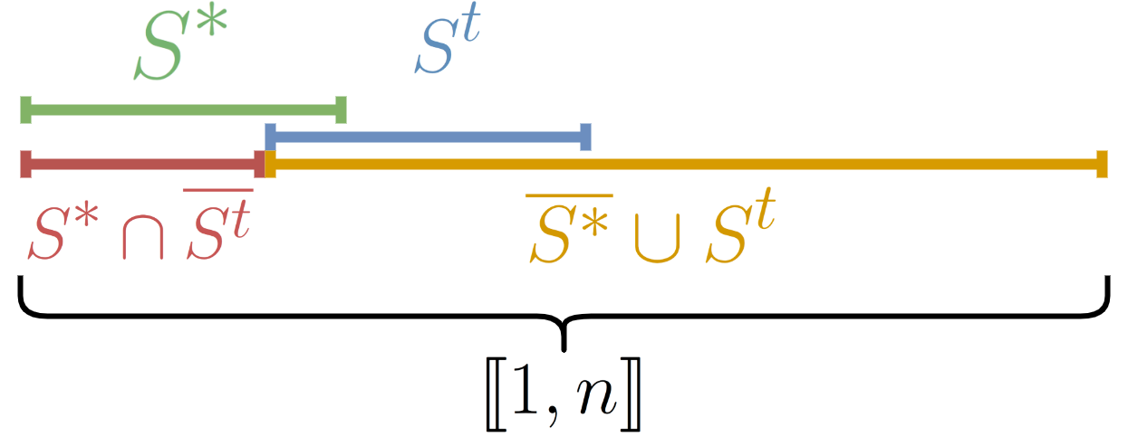
Figure 1: Visual representation of the main sets of indices encountered in the article.

The role of $\mathcal{X}^{t}$ may be intuited by first considering an oracle case where the true solution $x^{*}$and its support $S^{*}$ are known by the algorithm. In that case, at iteration $t$, we can use the oracle update rule $\mathcal{X}^{t+1}\leftarrow\mathcal{X}^{t}-u^{t}$, using the direction $u^{t}$ defined for any index $i$ by

$$u^{t}_{i}=\begin{cases}-\eta x^{*}_{i}&i\in S^{*}\cap\overline{S^{t}}\\ 0&i\in\overline{S^{*}}\cup S^{t},\end{cases}$$ (3)

where $S^{t}=\text{largest}_{k}\left(\mathcal{X}^{t}\right)$ is the indices of the $k$ largest absolute entries in $\mathcal{X}^{t}$ and $\eta>0$ is an arbitrary step size. We show the important supports in Figure 1. Notice $u^{t}_{i}$ is non-zero for indices $i$ from the true support $S^{*}$ but for which $|\mathcal{X}^{t}_{i}|$ is too small for $i$ to be in $S^{t}$. Whatever the initial content of $\mathcal{X}^{0}$, the oracle update rule always makes the same increment on $|\mathcal{X}^{t}_{i}|$, for $i\in S^{*}\cap\overline{S^{t}}$. This guarantees that, at some subsequent iteration $t^{\prime}\geq t$, the true support $S^{*}$ is recovered among the $k$ largest absolute entries in $\mathcal{X}^{t^{\prime}}$, i.e., $S^{*}\subset S^{t^{\prime}}$.

Since $x^{*}$ and $S^{*}$ are not available in practice, we replace the oracle update $u^{t}$ by the surrogate $\eta A^{T}(Ax^{t}-y)$ (see line 8). The choice of this surrogate is a natural one. For instance, one can show that $u^{t}=\eta A^{T}(Ax^{t}-y)$ in the simple case where $A$ is orthogonal and the observation is noiseless (see Corollary 3.2 and its proof in Appendix B). We will see in Theorem 3.3 and in its proof in Appendix C that $u^{t}-\eta A^{T}(Ax^{t}-y)$ is small, under suitable hypotheses on $x^{*}$ and the RIP constants of $A$.

An important feature of SEA is that it can be used as a post-processing of the solution $\hat{x}$ of another algorithm. This is simply done by initializing $\mathcal{X}^{0}=\hat{x}$. In this case $S^{0}=\text{supp}(\hat{x})$ (line 6) and $x^{0}$ improves or is equal to $\hat{x}$ (line 7). Since SEA returns the result obtained for the best time-step ${t_{BEST}}$ (line 11), it can only improve $\hat{x}$. In the experiments, we have investigated the initialization with the result of ELS [1, 30] and the initialization $\mathcal{X}^{0}=0$.

Eventually, the solution returned by SEA is selected at line 11 as the best iterate encountered along the iterations (see line 11). Of course, we do not compute ${t_{BEST}}$ after the ’repeat’ loop. We present it that way in Algorithm 1 for clarity only. In practice, we compute ${t_{BEST}}$ on the fly, after line 7. This way, computing ${t_{BEST}}$ and memorizing $x^{{t_{BEST}}}$ is done at no extra cost.

Finally, as often, there are many possible strategies to design the halting criterion of the ’repeat’ loop of Algorithm 1. It can for instance be based on the value of $\lVert Ax^{t}-y\rVert_{2}$ or on the values of $T_{max}$ established in the theorems of Section 3. We preferred to focus our experiments on the illustration of the potential benefits of SEA and, as a consequence, we have not investigated this aspect in the experiments and leave this study for the future. We always used a large fixed number of passes in the ’repeat’ loop of Algorithm 1.

Similarly, it is clear that $\eta$ (line 8) has no impact on $x^{t_{BEST}}$ when the algorithm is initialized with $\mathcal{X}^{0}=0$. In this case, indeed the whole trajectory $(\mathcal{X}^{t})_{t\in\mathbb{N}}$ is dilated by $\eta>0$ and the dilation has no effect on the selected supports $S^{t}$. When $\mathcal{X}^{0}\neq 0$, the initial support exploration variable is forgotten more or less rapidly depending on the value of $\eta$. This should have an effect on the output of the algorithm. As for the (related) halting criterion of the ’repeat’ loop of Algorithm 1, we have not studied the tuning of the step size $\eta$ and leave this study for future research.

2.3 Link with the straight-through estimator

The update of the support exploration variable $\mathcal{X}^{t}$ in SEA can be interpreted as a straight-through estimator [21, 4] (STE). An STE is used when optimizing a function $F$ that depends on a variable $x$ obtained in a non-differentiable way from another variable $\mathcal{X}$ as $x=H\left(\mathcal{X}\right)$. $\mathcal{X}$ is updated as $\mathcal{X}\leftarrow\mathcal{X}-\eta\frac{\partial F}{\partial x}$ by using, since $H$ is non-differentiable, the approximation at the core of STE: $\frac{\partial F}{\partial\mathcal{X}}=\frac{\partial F}{\partial x}\frac{\partial x}{\partial\mathcal{X}}\approx\frac{\partial F}{\partial x}$.

The STE has been successfully used in many applications where $H$ is a quantization. The STE had a very significant impact, for instance, on the optimization of neural networks over binary, ternary or more generally quantized weights [11, 22, 35].

The SEA algorithm is the STE applied to the resolution of (2) using the function $H:\mathbb{R}^{n}\longrightarrow\mathbb{R}^{n}$ defined by

$$H\left(\mathcal{X}\right)\in\underset{\begin{subarray}{c}x\in\mathbb{R}^{n}\\ \text{supp}(x)\subset\text{largest}_{k}\left(\mathcal{X}\right)\end{subarray}}{\operatorname{argmin}}\lVert Ax-y\rVert_{2}^{2}.$$

Using this definition, the solution of (2) are indeed of the form $H(\mathcal{X}^{*})$, for

$$\mathcal{X}^{*}\in\operatorname{argmin}_{\mathcal{X}}F(H(\mathcal{X})).$$

To the best of our knowledge, this is the first time the STE is used to solve a sparse linear inverse problem.

3 Theoretical analysis

We provide, in Section 3.1, the most general support recovery theorem stating that SEA recovers $S^{*}$ when $u^{t}$ and $\eta A^{T}(Ax^{t}-y)$ are close. We then specialize the theorem: 1/ to the noiseless case when $A$ is orthogonal; 2/ to the case of a matrix $A$ satisfying a RIP constraint in Section 3.2. In the latter statement, we obtain separate conditions on $A$ and $x^{*}$ that we compare with existing support recovery conditions, for the LASSO, OMP and HTP.

3.1 General recovery theorem

We remind that in Algorithm 1, replacing line 8 by the oracle update $\mathcal{X}^{t+1}=\mathcal{X}^{t}-u^{t}$, where $u^{t}$ is defined in (3), leads to an algorithm that recovers $S^{*}$. Since $u^{t}$ cannot be computed, we update $\mathcal{X}^{t}$ with a regular gradient step, see line 8 of Algorithm 1. For $t\in\mathbb{N}$, we define the gradient noise: $b^{t}\in\mathbb{R}^{n}$, the error between this computable dynamic and $u^{t}$ as

$$b^{t}=u^{t}-\eta A^{T}(Ax^{t}-y).$$ (4)

We define the maximal gradient noise norm

$$\varepsilon=\underset{\mathclap{t\in\mathbb{N}}}{\sup}\,\lVert b^{t}\rVert_{\infty}\in\mathbb{R}.$$ (5)

Finally, we define the Recovery Condition (RC) as

$$\varepsilon<\frac{1}{2\sum_{i\in S^{*}}\frac{1}{\eta\lvert x^{*}_{i}\rvert}}.$$ (RC)

Theorem 3.1 (Recovery - General case).

If (RC) holds, then for all initialisation $\mathcal{X}^{0}$ and all $\eta$, there exists $t_{s}\leq T_{max}$ such that $S^{*}\subset S^{t_{s}}$, where $S^{t}$ is defined in Algorithm 1 line 6 and

$$T_{max}=\frac{\sum_{i\in S^{*}}\frac{\max_{j\notin S^{*}}\lvert\mathcal{X}_{j}^{0}\rvert+\lvert\mathcal{X}_{i}^{0}\rvert}{\eta\lvert x^{*}_{i}\rvert}+k+1}{1-2\varepsilon\sum_{i\in S^{*}}\frac{1}{\eta\lvert x^{*}_{i}\rvert}}.$$ (6)

The proof is in Appendix A.

The main interest of Theorem 3.1 is to express clearly that, when $u^{t}-\eta A^{T}(Ax^{t}-y)$ is sufficiently small, SEA recovers the correct support. However, the condition (RC) is difficult to use and interpret since it involves both $A$, $x^{*}$ and all the sparse iterates $x^{t}$. This is why we particularize it in Corollary 3.2, Theorem 3.3 and Corollary 3.4.

The conclusion of Theorem 3.1 is that the iterative process of SEA recovers the correct support at some iteration $t$. We have in general no guarantee that this time-step $t$ is equal to ${t_{BEST}}$. We are however guaranteed that SEA returns a sparse solution such that $\lVert Ax^{{t_{BEST}}}-y\rVert_{2}\leq\lVert Ax^{*}-y\rVert_{2}$, which can be considered as a criterion of success. We will see in Corollary 3.2, Theorem 3.3 and Corollary 3.4 that, when $A$ is sufficiently incoherent and $\|e\|_{2}$ is small enough, we actually have $S^{*}\subset\text{supp}(x^{t_{BEST}})$.

Concerning the value of $T_{max}$, a quick analysis of the function $u\mapsto\frac{1}{1-au}$, for $a=2\sum_{i\in S^{*}}\frac{1}{\eta\lvert x^{*}_{i}\rvert}>0$ and for $u<1/a$ shows that $T_{max}$ increases with $\varepsilon$, when (RC) holds. In other words, the number of iterations required by the algorithm to provide the correct solution increases with the discrepancy between $u^{t}$ and $\eta A^{T}(Ax^{t}-y)$. This confirms the intuition behind the construction of SEA. The initializations $\mathcal{X}^{0}\neq 0$ have an apparent negative impact on the number of iterations required in the worst case. This is because in the worst-case $\mathcal{X}^{0}$ would be poorly chosen and SEA needs iterations to correct this poor choice. However, we can expect a well-chosen initialization of $\mathcal{X}^{0}$ to reduce the number of iterations required by SEA to recover the correct support.

Concerning $\eta$, notice that, since $u^{t}$ is proportional to $\eta>0$, $\varepsilon$ is proportional to $\eta>0$ and therefore (RC) is independent of $\eta$. When possible, any $\eta$ permits to recover $S^{*}$. The only influence of $\eta$ is on $T_{max}$. In this regard, since $\varepsilon$ is proportional to $\eta>0$, $\eta$ has no influence on the denominator of (6). It only influences the numerator of (6). In this numerator, we see that the larger $\eta$ is, the faster SEA will override the initialization $\mathcal{X}^{0}$. This is very much related to the question of the quality of the initialization discussed above.

The following corollary particularizes Theorem 3.1 to the noiseless and orthogonal case. In practice, a complicated algorithm like SEA is of course useless in such a case. We give this corollary mostly to illustrate the diversity of links between the properties of the triplet $(A,x^{*},e)$ and $\varepsilon$ and the behavior of SEA.

Corollary 3.2 (Recovery - Orthogonal case).

If $A$ is an orthogonal matrix ($A^{-1}=A^{T}$) and $\lVert e\rVert_{2}=0$, then

$$\varepsilon=0.$$

As a consequence, for all $x^{*}$, for initialisation $\mathcal{X}^{0}=0_{\mathbb{R}^{n}}$ and all $\eta$, if SEA performs more than $k+1$ iterations, we have

$$S^{*}\subset S^{{t_{BEST}}}\qquad\mbox{and}\qquad x^{{t_{BEST}}}=x^{*}.$$

The proof is in Appendix B.

3.2 Recovery theorem in the RIP case

In this section, we assume that for any $i\in\llbracket 1,n\rrbracket$, $\lVert A_{i}\rVert_{2}=1$. As is standard since it has been proposed by Candès and Tao in [9], we define for all $l\in\llbracket 1,n\rrbracket$ the $l$th Restricted Isometry Constant of $A$ as the smallest non-negative number $\delta_{l}$ such that for any $x\in\mathbb{R}^{n}$, $\lVert x\rVert_{0}\leq l$,

$$(1-\delta_{l})\lVert x\rVert_{2}^{2}\leq\lVert Ax\rVert_{2}^{2}\leq(1+\delta_{l})\lVert x\rVert_{2}^{2}.$$ (7)

If $\delta_{l}<1$, $A$ is said to satisfy the Restricted Isometry Property of order $l$ or the $l$-RIP.

In this section, we assume that $A$ satisfies the $(2k+1)$-RIP. In the scenarios of interest, $\delta_{2k+1}$ is small. We define,

$$\alpha^{\scriptscriptstyle RIP}_{k}=\delta_{2k+1}\left(\frac{\delta_{2k}}{1-\delta_{k}}+1\right)\in\mathbb{R}^{*}_{+}$$ (8)

and

$$\gamma^{\scriptscriptstyle RIP}_{k}=\delta_{2k+1}\frac{\sqrt{1+\delta_{k}}}{1-\delta_{k}}+1\in\mathbb{R}^{*}_{+}.$$ (9)

As soon as $\delta_{k}$ is far from $1$, which will be the case in the scenarios of interest, $\alpha^{\scriptscriptstyle RIP}_{k}$ has the order of magnitude $\delta_{2k+1}$ and $\gamma^{\scriptscriptstyle RIP}_{k}$ has the order of magnitude of $1+\delta_{2k+1}$.

As is common for support recovery statements, the next theorem involves a condition on $x^{*}$. It is indeed impossible to recover an element $i$ of $S^{*}$ if $x^{*}_{i}$ is negligible compared to the other quantities of (1). We call this condition the Recovery Condition for the RIP case ($\textit{RC}_{\scriptscriptstyle RIP}$). It is defined by

$$\gamma^{\scriptscriptstyle RIP}_{k}\lVert e\rVert_{2}<\frac{1}{2\sum_{i\in S^{*}}\frac{1}{\lvert x^{*}_{i}\rvert}}-\alpha^{\scriptscriptstyle RIP}_{k}\lVert x^{*}\rVert_{2}. \textit{RC}_{\scriptscriptstyle RIP}$$ ()

If ($\textit{RC}_{\scriptscriptstyle RIP}$) holds, $x^{*}$ is said to satisfy the ($\textit{RC}_{\scriptscriptstyle RIP}$) condition.

Theorem 3.3 (Recovery - RIP case).

Assume $A$ satisfies the $(2k+1)$-RIP and for all $i\in\llbracket 1,n\rrbracket$, $\lVert A_{i}\rVert_{2}=1$. Then

$$\varepsilon\leq\eta(\alpha^{\scriptscriptstyle RIP}_{k}\|x^{*}\|_{2}+\gamma^{\scriptscriptstyle RIP}_{k}\|e\|_{2}).$$

If moreover $x^{*}$ satisfies ($\textit{RC}_{\scriptscriptstyle RIP}$), then for all initialisation $\mathcal{X}^{0}$ and all $\eta$, there exists $t_{s}\leq T_{\scriptscriptstyle RIP}$ such that $S^{*}\subset S^{t_{s}}$, where

$$T_{\scriptscriptstyle RIP}=\frac{\sum_{i\in S^{*}}\frac{\max_{j\notin S^{*}}\lvert\mathcal{X}_{j}^{0}\rvert+\lvert\mathcal{X}_{i}^{0}\rvert}{\eta\lvert x^{*}_{i}\rvert}+k+1}{1-2(\alpha^{\scriptscriptstyle RIP}_{k}\lVert x^{*}\rVert_{2}+\gamma^{\scriptscriptstyle RIP}_{k}\lVert e\rVert_{2})\sum_{i\in S^{*}}\frac{1}{\lvert x^{*}_{i}\rvert}}.$$ (10)

If moreover, $x^{*}$ is such that

$$\min_{i\in S^{*}}|x^{*}_{i}|>\frac{2}{\sqrt{1-\delta_{2k}}}\|e\|_{2}$$ (11)

and SEA performs more than $T_{\scriptscriptstyle RIP}$ iterations, then

$$S^{*}\subset S^{{t_{BEST}}}~{}~{}~{}~{}\mbox{and}~{}~{}~{}~{}\|x^{{t_{BEST}}}-x^{*}\|_{2}\leq\frac{2}{\sqrt{1-\delta_{k}}}\|e\|_{2}.$$

The proof is in Appendix C.

The hypotheses of the theorem are on the RIP of $A$ and there are two hypotheses on $x^{*}$: ($\textit{RC}_{\scriptscriptstyle RIP}$) and (11). The condition ($\textit{RC}_{\scriptscriptstyle RIP}$) is difficult to interpret. Below, we give an example to illustrate it.

The first example is when for all $i\in S^{*}$, $x^{*}_{i}=c$ for some constant $c\in\mathbb{R}$. Condition ($\textit{RC}_{\scriptscriptstyle RIP}$) becomes in this case

$$\gamma^{\scriptscriptstyle RIP}_{k}\|e\|_{2}\leq|c|\left(\frac{1-2\alpha^{\scriptscriptstyle RIP}_{k}|S^{*}|^{\frac{3}{2}}}{2|S^{*}|}\right).$$

This can only hold under the condition that $\alpha^{\scriptscriptstyle RIP}_{k}\leq\frac{1}{2|S^{*}|^{\frac{3}{2}}}$, where we remind that $\alpha^{\scriptscriptstyle RIP}_{k}$ has the order of magnitude of $\delta_{2k+1}$ and $|S^{*}|\leq k$. If this condition on the RIP of $A$ holds, any value of $c$ satisfying

$$|c|\geq\left(\frac{2\gamma^{\scriptscriptstyle RIP}_{k}|S^{*}|}{1-\alpha^{\scriptscriptstyle RIP}_{k}|S^{*}|^{\frac{3}{2}}}\right)\|e\|_{2}$$

leads to an $x^{*}$ that satisfies ($\textit{RC}_{\scriptscriptstyle RIP}$). Notice, that in this particular example, a rapid analysis shows that ($\textit{RC}_{\scriptscriptstyle RIP}$) is a stronger requirement than (11).

To illustrate ($\textit{RC}_{\scriptscriptstyle RIP}$), we provide below a simplified condition which is shown in Corollary 3.4 to be stronger than ($\textit{RC}_{\scriptscriptstyle RIP}$) in the noiseless scenario. We say $x^{*}$ satisfies the Simplified Recovery Condition in the RIP case if there exist $\Lambda\in(0,1)$ such that

$$2k\alpha^{\scriptscriptstyle RIP}_{k}\frac{\lVert x^{*}\rVert_{2}}{\min_{i\in S^{*}}\lvert x^{*}_{i}\rvert}\leq\Lambda. \textit{S}\textit{RC}_{\scriptscriptstyle RIP}$$ ()

Corollary 3.4 (Noiseless recovery - simplified RIP case).

Assume $\lVert e\rVert_{2}=0$, $A$ satisfies the $(2k+1)$-RIP and for all $i\in\llbracket 1,n\rrbracket$, $\lVert A_{i}\rVert_{2}=1$.

If moreover $x^{*}$ satisfies ($\textit{S}\textit{RC}_{\scriptscriptstyle RIP}$), then $x^{*}$ satisfies ($\textit{RC}_{\scriptscriptstyle RIP}$). As a consequence, for all $x^{*}$, for initialisation $\mathcal{X}^{0}=0_{\mathbb{R}^{n}}$ and all $\eta$, if SEA performs more than

$$T_{\scriptscriptstyle RIP}^{\prime}=\frac{k+1}{1-\Lambda}$$ (12)

iterations, we have

$$S^{*}\subset S^{{t_{BEST}}}\qquad\mbox{and}\qquad x^{{t_{BEST}}}=x^{*}.$$

The proof is in Section C.4.

Notice that if $\alpha^{\scriptscriptstyle RIP}_{k}$ is too large, there does not exist any $x^{*}$ satisfying ($\textit{S}\textit{RC}_{\scriptscriptstyle RIP}$). It is for instance the case if $\alpha^{\scriptscriptstyle RIP}_{k}\geq 0.5$. On the contrary, a sufficient condition of existence of vectors $x^{*}$ satisfying ($\textit{S}\textit{RC}_{\scriptscriptstyle RIP}$) is that the constant $\alpha^{\scriptscriptstyle RIP}_{k}$ satisfies $2k^{\frac{3}{2}}\alpha^{\scriptscriptstyle RIP}_{k}\leq\Lambda<1$. In this case, when all the entries of $x^{*}$ are equal, we have $\|x^{*}\|_{2}=\sqrt{|S^{*}|}\min_{i\in S^{*}}\lvert x^{*}_{i}\rvert$ and

$$2k\alpha^{\scriptscriptstyle RIP}_{k}\frac{\lVert x^{*}\rVert_{2}}{\min_{i\in S^{*}}\lvert x^{*}_{i}\rvert} = 2k\alpha^{\scriptscriptstyle RIP}_{k}\sqrt{|S^{*}|}$$

$$\leq 2k^{\frac{3}{2}}\alpha^{\scriptscriptstyle RIP}_{k}\leq\Lambda<1.$$

When this holds, the set of $x^{*}$ satisfying ($\textit{S}\textit{RC}_{\scriptscriptstyle RIP}$) is a convex cone whose interior is not empty. The set grows as $\alpha^{\scriptscriptstyle RIP}_{k}$ decreases.

Compared to the support recovery guarantees in the noisy case for the LASSO [32, 26, 34], the OMP [7], the HTP [19, 33] and the ARHT [1] the recovery conditions provided in Theorem 3.3 and Corollary 3.4 for SEA seem stronger. All conditions involve a condition on the incoherence of $A$ and a condition similar to (11). In the case of the LASSO algorithm, the latter is not very explicit. However, none of the support recovery conditions involve a condition like ($\textit{RC}_{\scriptscriptstyle RIP}$) and ($\textit{S}\textit{RC}_{\scriptscriptstyle RIP}$). A clear drawback of these conditions is that the support of an $x^{*}$ such that $\max_{i\in S^{*}}|x^{*}_{i}|\gg\min_{i\in S^{*}}|x^{*}_{i}|$ is not guaranteed to be recovered. This is because, if $i\not\in S^{t}$ and $|x^{*}_{i}|\gg\min_{i\in S^{*}}|x^{*}_{i}|$, $b^{t}$ can be large. However, it is possible to get around this problem since SEA inherits the support recovery properties of any well-chosen initialization. Also, we have not observed this phenomenon in the experiments of Section 4. Similarly, SEA performs well even when $A$ is coherent, see Section 4.2. This is not explained by Theorem 3.3 and Corollary 3.4 which consider the classical RIP assumption.

Improving the theoretical analysis in these directions is left for the future. The current statements permit to see that SEA is a sound algorithm. To the best of our knowledge, this is the first time such guarantees are given for an algorithm based on the STE.

4 Experimental analysis

We compare SEA to state-of-the-art algorithms on three tasks: Extensive signal recovery through phase transition diagram in Section 4.1, spike deconvolution problems for signal processing in Section 4.2 and linear regression and logistic regression tasks in supervised learning settings in Section 4.3.

The tested algorithms are IHT [6], OMP [25, 28], OMPR [23] and ELS [1] (a.k.a. Fully Corrective Forward Greedy Selection with Replacement [30]). OMPR and ELS are initialized with the solution of OMP. Two versions of SEA are studied: the cold-start version SEA${}_{\text{0}}$, where SEA is initialized with the null vector and the warm-start version SEA${}_{\text{ELS}}$, where SEA is initialized with the solution of ELS.

For all algorithms, each least-square projection for a fixed support, as in Line 7 of Algorithm 1, is solved using the conjugate gradient descent of scikit-learn [29]. The maximal number of iterations is $256k$. Matrix $A$ is normalized before solving the problem. For each experiment, appropriate metrics, defined in the relevant subsection, are used for performance evaluation. The code is implemented in Python 3 and is available in the git repository of the project .

4.1 Phase transition diagram experiment

Phase transition diagram experiment is an extensive experiment commonly used for algorithm performance comparison over synthetic data. Introduced by Donoho and Tanner in [14], phase transition diagrams show the recovery limits of an algorithm depending on the undersampling/indeterminacy $\zeta=\frac{m}{n}$ of $A$, and the sparsity/density $\rho=\frac{k}{m}$ of $x^{*}$. We consider the noiseless setup (i.e., $e=0_{\mathbb{R}^{m}}$ in (1)). We fix $n=64$, $m$ takes all values in $\llbracket 9,n\rrbracket$ and $k$ all values in $\llbracket 9,m\rrbracket$. For each triplet $(m,n,k)$ and each algorithm, we run $r=1000$ experiments (described below) to assess the success rate $\frac{s_{\zeta,\rho}}{r}$ of the algorithm, where $s_{\zeta,\rho}$ is the number of problems successfully solved. A problem is considered successfully solved if the support of the output of the algorithm contains $S^{*}$.

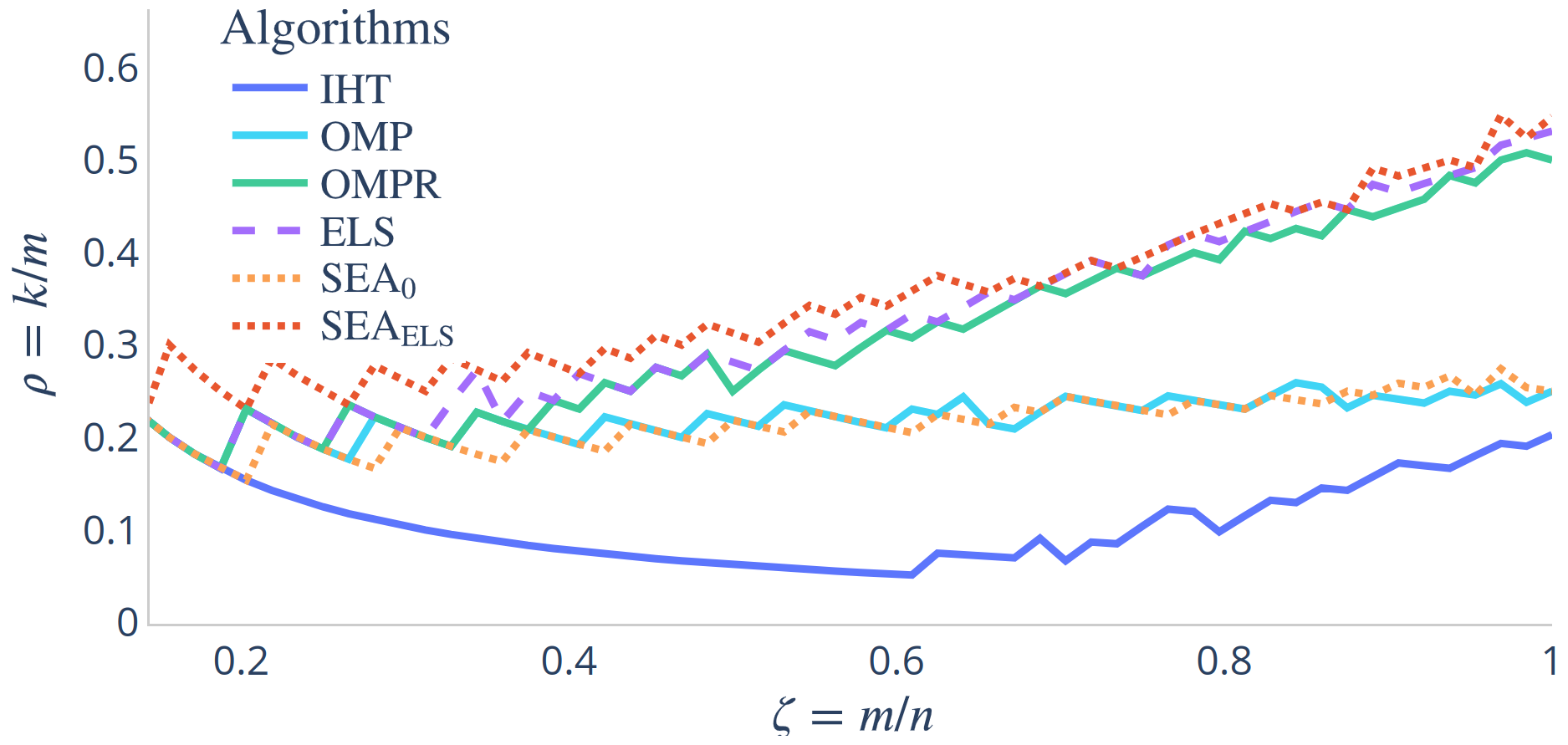
Figure 2: Empirical support recovery phase transition curves. Problems below each curve are solved by the related algorithm with a success rate larger than $95\%$.

For a triplet $(m,n,k)$ and an algorithm, the matrix $A\in\mathbb{R}^{m\times n}$ is a Gaussian matrix. Its entries are drawn independently from the normal distribution ${\mathcal{N}}(0,1)$. The restricted isometry constants are poor when $\zeta=\frac{m}{n}$ is small and improve when $m$ grows [2].

The sparse vector $x^{*}\in\mathbb{R}^{n}$ is random. Indexes of the support are randomly picked, uniformly without replacement. The non-zero entries of $x^{*}$ are independently drawn from the standard normal distribution.

Figure 2 shows results from this experiment. Each colored curve indicates the threshold below which the algorithm has a success rate larger than $95\%$. We see that IHT achieves poor recovery successes, which are only located at small values of sparsity $k$. SEA${}_{\text{0}}$ is on par with OMP. OMPR and ELS improve OMP performances, in particular, when $\frac{m}{n}\geq 0.5$, i.e. when matrices $A$ are less coherent. SEA${}_{\text{ELS}}$ improves further ELS performances and outperforms the other algorithms for all $\frac{m}{n}$. The largest improvement is for $\frac{m}{n}=0.65$, which corresponds to the most coherent matrices $A$. Thus, SEA refines a good support candidate into a better one by exploring new supports and achieves recovery for higher values of sparsity $k$ than competitors. The actual superiority of SEA${}_{\text{ELS}}$ for coherent matrices ($\zeta<0.65$) is particularly remarkable and illustrates its ability to successfully explore supports in difficult problems where competitors fail. We study the noisy setup (i.e., $e\neq 0_{\mathbb{R}^{m}}$ in (1)) in Appendix D.

4.2 Deconvolution experiment

Deconvolution purposes arise in many signal processing areas among which are microscopy or remote sensing. Of particular interest here is the deconvolution of sparse signals, also known as point source deconvolution [5] or spike deconvolution [17, 16], assuming the linear operator is known (contrary to blind approaches [24]). The objective is thus here to recover spike positions and amplitudes.

We consider the noiseless setup (i.e., $e=0_{\mathbb{R}^{m}}$ in (1)). We choose $n=64$, a convolution matrix $A$ corresponding to a Gaussian filter with a standard deviation equal to $3$. The coherence of the matrix $A$ is $\max_{i\neq j}|A_{i}^{T}A_{j}|=0.97$. The problem is therefore very difficult and the support recovery theorems do not apply.

For each sparsity level $k\in\llbracket 1,16\rrbracket$, every algorithm is tested on $r=1000$ different noiseless problems corresponding to different $k$-sparse $x^{*}$. The maximal number of iterations is $1000$, for all algorithms. The $k$-sparse vector $x^{*}$ is random. Its support is drawn uniformly without replacement and its non-zero entries are drawn uniformly in $[-2,-1]\cup[1,2]$ as in [18].

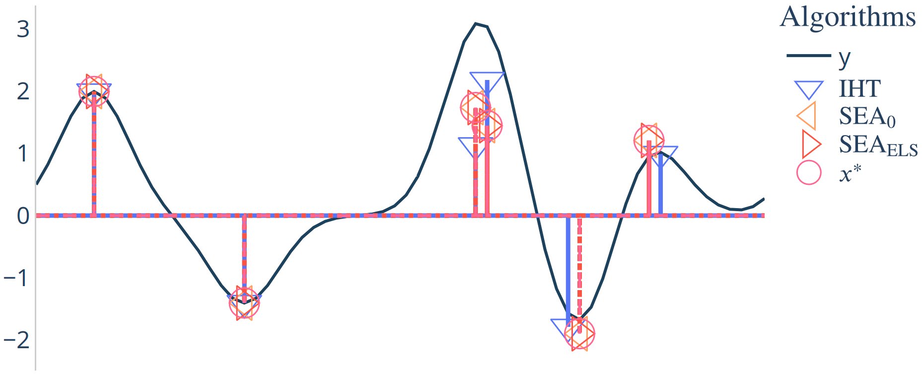
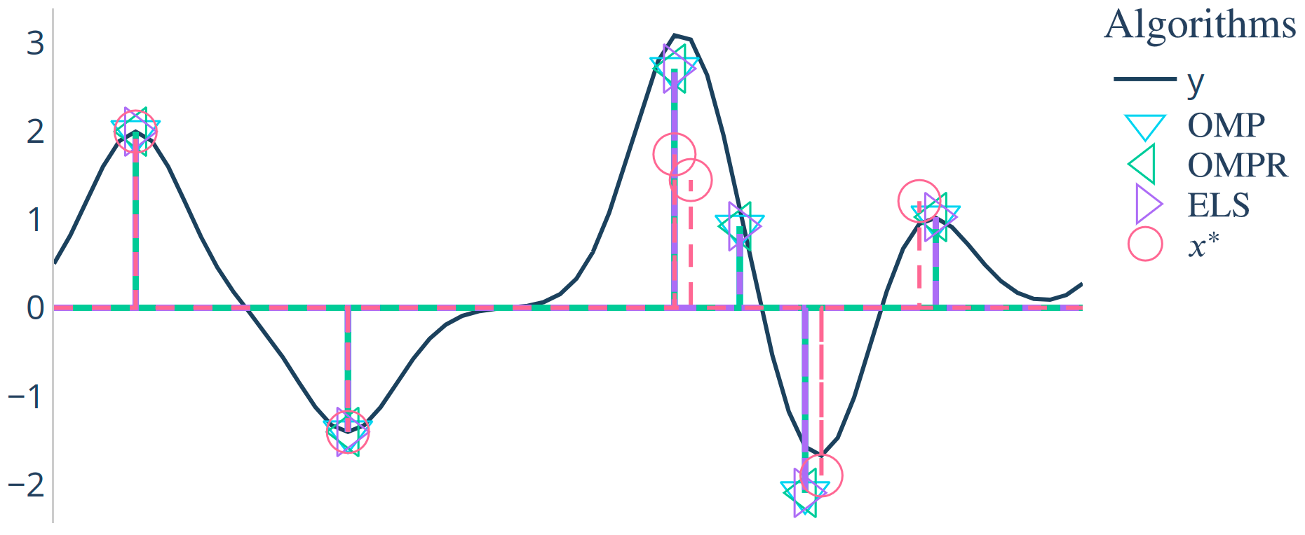
Figure 3: Representation of an instance of $x^{*}$ and $y$ with the solutions provided by the algorithms when $k=6$. Results are reported in two axes for clarity.

Figure 3 illustrates the results for a $6$-sparse vector $x^{*}$. Isolated spikes are located by all algorithms. However, the closer the spikes, the harder to locate them for algorithms. Both SEA${}_{\text{0}}$ and SEA${}_{\text{ELS}}$ are able to recover the original signal, while other algorithms fail. In Section E.1, we give for the experiment of Figure 3 the evolution of $\lVert Ax^{t}-y\rVert_{2}$ when $t$ varies, for SEA${}_{\text{0}}$ and SEA${}_{\text{ELS}}$.

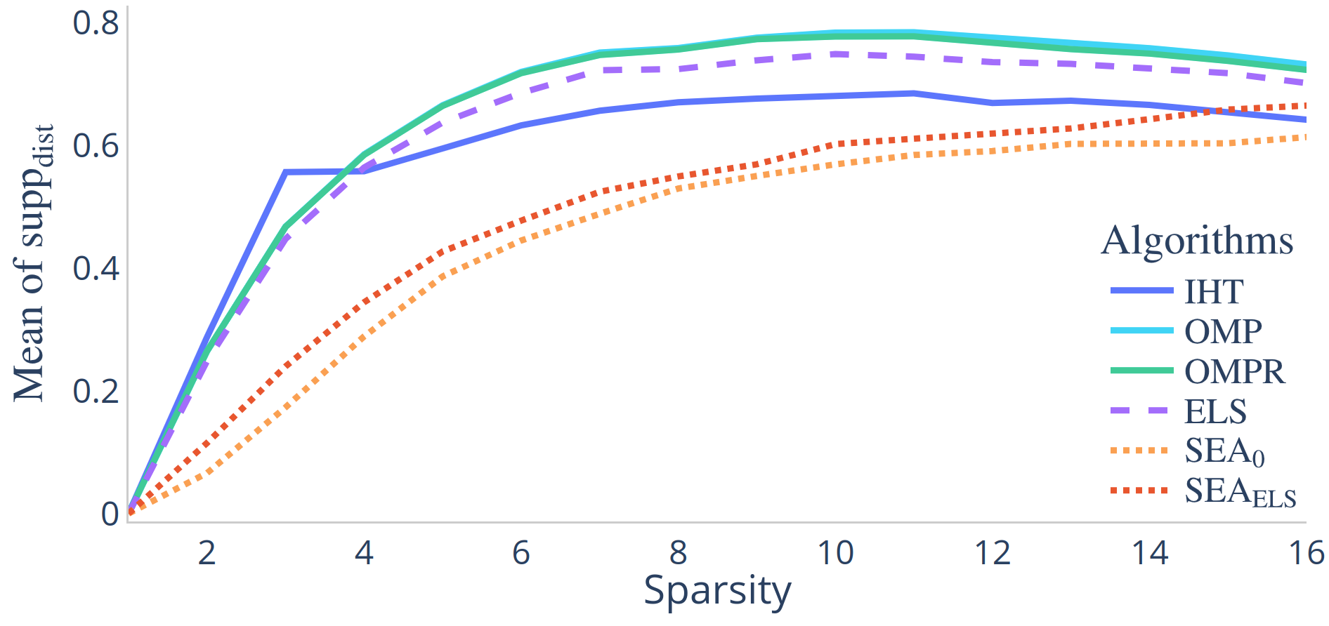
Figure 4: Mean of support distance $\text{supp}_{\text{dist}}$ between $S^{*}$ and the support of the solutions provided by several algorithms as a function of the sparsity level $k$.

On Figure 4, the performance of each algorithm is reported, for all $k\in\llbracket 1,16\rrbracket$, by the average over $r$ runs of the support distance metric [18] defined by

$$\text{supp}_{\text{dist}}(x)=\frac{k-\lvert S^{*}\cap\ \text{supp}(x)\rvert}{k}.$$ (13)

For sparsity $k<14$, SEA${}_{\text{0}}$ and SEA${}_{\text{ELS}}$ outperform the other algorithms. By exploring various supports, SEA finds better supports than its competitors. As $k$ increases, due to the increasing difficulty of the problem, no algorithm is able to recover $S^{*}$. We provide additional experiments in Appendix E, leading to the same conclusions.

4.3 Supervised learning experiment

In a supervised learning setting, matrix $A\in\mathbb{R}^{m\times n}$ (often denoted by $X$) contains $m$ $n$-dimensional feature vectors associated with the training examples and arranged in rows, while the related labels are in vector $y\in\mathbb{R}^{m}$. In the training phase, a sparse vector $x$ (often denoted $\beta$ or $w$) is optimized to fit $y\approx Ax$ using an appropriate loss function: in this context, support recovery is called model selection.

Based on the experimental setup of [1], we compare all the algorithms on linear regression and logistic regression tasks in terms of loss over the training set for different levels of sparsity. We use the preprocessed public datasets provided by  [1], following the same preprocessing pipeline: we augment $A$ with an extra column equal to $1_{\mathbb{R}^{m}}$ to allow a bias and normalize the columns of $A$.

For regression problems we use the $\ell_{2}$ regression loss defined by $\ell_{2}\_\text{loss}(x)=\frac{1}{2}\lVert Ax-y\rVert_{2}^{2}$ for $x\in\mathbb{R}^{n}$.

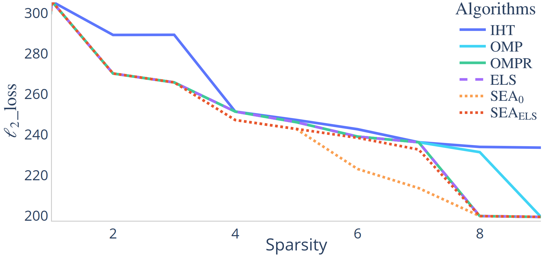
Figure 5: Performance on the regression dataset cal_housing ($m=20639$ examples, $n=8$ features).

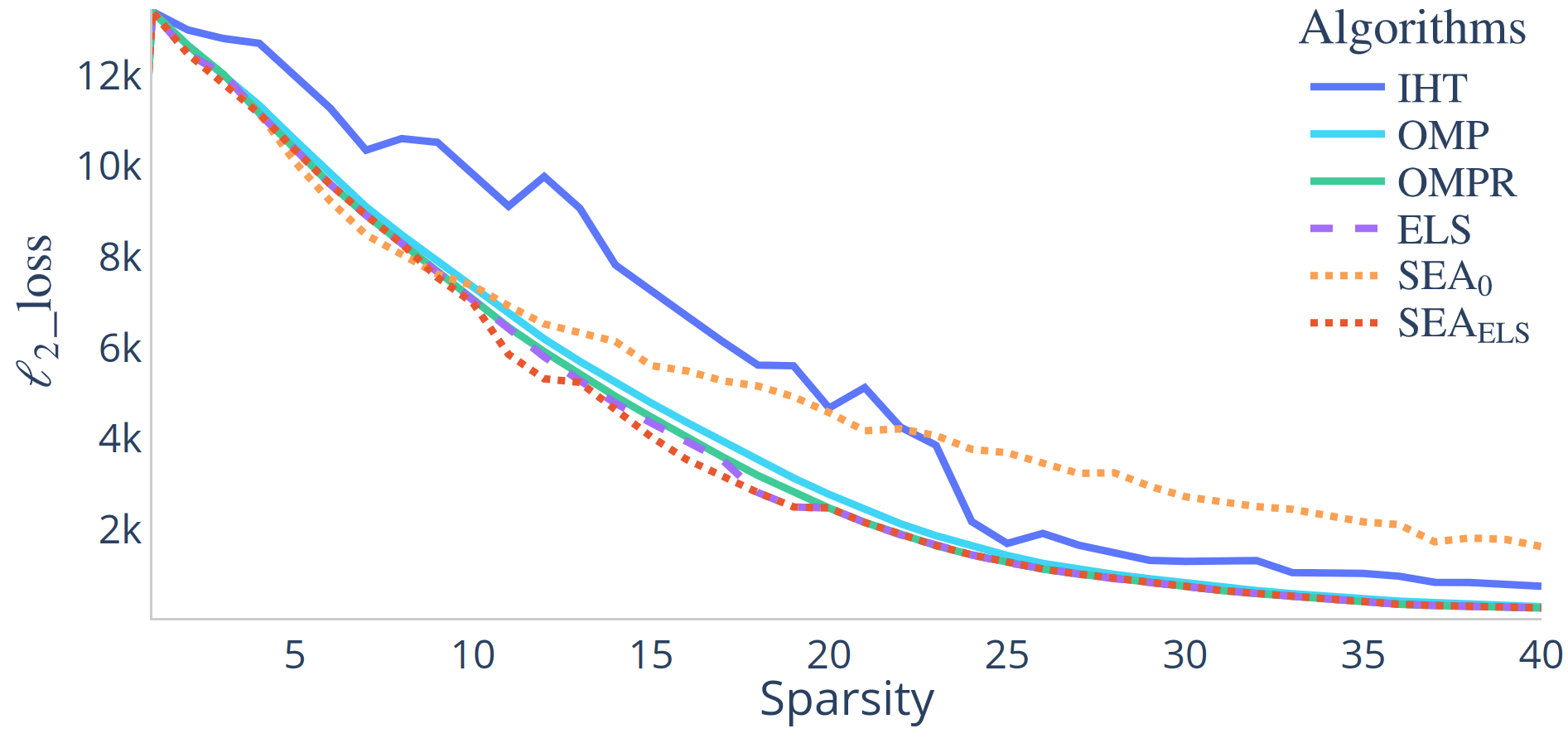
Figure 6: Performance on the regression dataset year ($m=463715$ examples, $n=90$ features).

As shown in Figure 5, SEA${}_{\text{0}}$ and SEA${}_{\text{ELS}}$  outperform the other algorithms on a regression dataset with $n$ small. For a regression dataset in a higher dimension, as shown in Figure 6, SEA${}_{\text{0}}$ performs poorly as $k$ increases. In both cases, SEA${}_{\text{ELS}}$ is able to increase further ELS performances and outperforms the other algorithms.

As confirmed in Appendix F by the experiments on other regression and binary classification datasets, SEA${}_{\text{0}}$ performs well in small dimensions, while a good initialization is mandatory in higher dimensions.

These experiments give some evidence that SEA can perform very well when some error/noise is present in the observation and when no perfect sparse vector exists.

5 Conclusion and perspectives

In this article, we proposed SEA: a new principled algorithm for sparse support recovery, based on STE. We established guarantees when the matrix $A$ satisfies the RIP. Experiments show that SEA supplements state-of-the-art algorithms and outperforms them in particular when $A$ is coherent.

The theoretical guarantees involve conditions on $x^{*}$ that are not present for similar statements for other algorithms and that might restrict its applicability. Also, the algorithm seems to perform well when $A$ is coherent and this is not explained by the current theoretical analysis which only applies to matrices satisfying the RIP. Improving the theoretical analysis in these directions are promising perspective.

There are many perspectives of applications of SEA and the STE to sparse inverse problems such as sparse matrix factorization, tensor problems, as well as real-world applications for instance in biology and astronomy.

Finally, it would be interesting to investigate the adaptation of the methods developed in this article to other applications of STE, such as BinaryConnect.

6 Acknowledgement

This work has benefited from the AI Interdisciplinary Institute ANITI, which is funded by the French “Investing for the Future – PIA3” program under the Grant agreement ANR-19-P3IA-0004. F. Malgouyres gratefully acknowledges the support of IRT Saint Exupéry and the DEEL project and thanks Franck Mamalet for all the discussions on the STE.

M. Mohamed was suppported by a PhD grant from ”Emploi Jeunes Doctorants (EJD)” plan which is funded by the French institution ”Région Sud - Provence-Alpes-Côte d’Azur” and Euranova France. M. Mohamed gratefully acknowledges their financial support.

Appendix A Proof of Theorem 3.1

To prove Theorem 3.1, we need to find a closed formula for the exploratory variable $\mathcal{X}^{t}$. Then, we will study the properties of this closed formula through the counting vector $c^{t}$ to find a sufficient condition of support recovery.

A.1 Preliminary 1: Closed formulation of $\mathcal{X}^{t}$

Before the proof, we remind Figure 1 in Figure 7.

Figure 7: Visual representation of the main sets of indices encountered in the article.

For each iteration $t\in\mathbb{N}$ and $i\in\llbracket 1,n\rrbracket$, we also remind the oracle update already defined in (3)

$$u^{t}_{i}=\begin{cases}-\eta x^{*}_{i}&i\in S^{*}\cap\overline{S^{t}}\\ 0&i\in\overline{S^{*}}\cup S^{t}.\end{cases}$$

We also remind the gradient noise, already defined in (4), $b^{t}=u^{t}-\eta A^{T}(Ax^{t}-y)$. We remark that, for any $i\in S^{t}$, $b^{t}_{i}=0$. Indeed, we have, for all $i\in S^{t}$, $u^{t}_{i}=0$ and $(A^{T}(Ax^{t}-y))_{i}=0$, the latter being a consequence of the definition of $x^{t}$ in Algorithm 1, line 7.

As a consequence of the definition of $b^{t}$ and SEA, line 8, for any $t\in\mathbb{N}$,

$$\mathcal{X}^{t+1}=\mathcal{X}^{t}+b^{t}-u^{t}.$$ (14)

The gradient noise $b^{t}$ is the error preventing the gradient from being in the direction of the oracle update $u^{t}$. At each iteration, this error is accumulating in $\mathcal{X}^{t}$. With $\beta^{0}=0_{\mathbb{R}^{n}}$, for any $t\in\mathbb{N}^{*}$, we define this accumulated error by

$$\beta^{t}=\sum_{{t^{\prime}}=0}^{t-1}b^{t^{\prime}}\in\mathbb{R}^{n}.$$ (15)

With $c^{0}=0_{\mathbb{R}^{n}}$, for any $t\in\mathbb{N}^{*}$ and $i\in\llbracket 1,n\rrbracket$, we also define the counting vector by

$$c_{i}^{t}=\lvert\{{t^{\prime}}\in\llbracket 0,t-1\rrbracket:i\in S^{*}\cap\overline{S^{{t^{\prime}}}}\}\rvert.$$ (16)

We will use the recursive formula for $c^{t}$: For any $t\in\mathbb{N}$, $i\in\llbracket 1,n\rrbracket$

$$c_{i}^{t+1}=\begin{cases}c_{i}^{t}+1&\mbox{if }i\in S^{*}\cap\overline{S^{t}}\\ c_{i}^{t}&\mbox{if }i\in\overline{S^{*}}\cup S^{t}.\end{cases}$$ (17)

For any $i\in\llbracket 1,n\rrbracket$, the sequence $(c_{i}^{t})_{t\in\mathbb{N}}$ is non-decreasing.

We write a closed formula for the exploratory variable $\mathcal{X}^{t}$.

Proposition A.1 (Counting).

For any $t\in\mathbb{N}$, $\mathcal{X}^{t}=\mathcal{X}^{0}+\eta c^{t}\odot x^{*}+\beta^{t}$, where $\odot$ denotes the Hadamard product.

We omit the details but, using (14), (15) and (16), the proposition is proved by induction on t.

A.2 Preliminary 2: Counting vector behavior

As can be seen from Proposition A.1, the error accumulation $\beta^{t}$ is responsible for the exploration in wrong directions. While $c^{t}\odot x^{*}$ encourages exploration in the direction of the missed components of $x^{*}$. Here, we describe the behavior of $(c^{t})_{t\in\mathbb{N}}$.

At each iteration of SEA, using (17) when $S^{*}\nsubseteq S^{t}$, at least one coordinate of the counting vector is increased by one. Since, for all $i\in\llbracket 1,n\rrbracket$, $(c_{i}^{t})_{t\in\mathbb{N}}$ is non-decreasing, we obtain the following Lemma.

Lemma A.2 (Increase).

For any $t\in\mathbb{N}$ such that $S^{*}\nsubseteq S^{t}$, $\sum_{i\in S^{*}}c_{i}^{t+1}\geq\left(\sum_{i\in S^{*}}c_{i}^{t}\right)+1$.

We define the first recovery iterate by

$${t_{s}}=\min{\{t,\,S^{*}\subseteq S^{t}\}\in\mathbb{N}}.$$ (18)

By convention, if $S^{*}$ is never recovered, ${t_{s}}=+\infty$.

By induction on $t$, using Lemma A.2, we obtain a lower bound on $\sum_{i\in S^{*}}c_{i}^{t}$.

Corollary A.3 (Lower bound).

For any $t\leq{t_{s}}$, $\sum_{i\in S^{*}}c_{i}^{t}\geq t$.

Let us now upper bound $\sum_{i\in S^{*}}c_{i}^{t}$. We first remind the definition of $\varepsilon$ in (5), the Recovery Condition (RC) and the value of $T_{max}$ in (6) in Theorem 3.1. If (RC) holds, we define for any $i\in S^{*}$, the $i^{th}$ counting threshold by

$$C_{i}=\frac{\max_{j\notin S^{*}}\lvert\mathcal{X}_{j}^{0}\rvert+\lvert\mathcal{X}_{i}^{0}\rvert+2T_{max}\varepsilon}{\eta\lvert x^{*}_{i}\rvert}.$$ (19)

Proposition A.4 (Upper bound).

If (RC) holds, for any $i\in S^{*}$ and any $t\leq T_{max}$, we have $c_{i}^{t}\leq C_{i}+1$.

Proof.

Assume (RC) holds. We have $T_{max}>0$. Let $i\in S^{*}$, we distinguish two cases:

$1^{st}\,case$: If for all $t\leq T_{max}$, $c_{i}^{t}\leq C_{i}$: Then, obviously, for any $t\leq T_{max}$, $c_{i}^{t}\leq C_{i}+1$.

$2^{nd}\,case$: If there exists $t\leq T_{max}$, such that $c_{i}^{t}>C_{i}$:

We define ${t_{i}}=\min{\{t\in\mathbb{N}:\,c_{i}^{t}>C_{i}\}}$. We have ${t_{i}}\leq T_{max}$. The proof follows two steps:

$$\text{\hskip 4.83691pt 1. We will prove that for all }t\in\llbracket{t_{i}},T_{max}\rrbracket,\,c_{i}^{t}=c_{i}^{t_{i}}.$$ (20)

$$\text{\hskip 4.83691pt 2. We will prove that for all }t\leq T_{max},\,c_{i}^{t}\leq C_{i}+1.$$ (21)

1. Let $t\in\llbracket{t_{i}},T_{max}\rrbracket$, we have, using Proposition A.1, the triangle inequality and the fact that $c_{i}^{t}\geq c_{i}^{t_{i}}>C_{i}$

   $$\lvert\mathcal{X}_{i}^{t}\rvert =\lvert\mathcal{X}_{i}^{0}+\eta c_{i}^{t}x^{*}_{i}+\beta_{i}^{t}\rvert$$

   $$\geq\eta c_{i}^{t}\lvert x^{*}_{i}\rvert-\lvert\mathcal{X}_{i}^{0}\rvert-\lvert\beta_{i}^{t}\rvert$$

   $$>\eta C_{i}\lvert x^{*}_{i}\rvert-\lvert\mathcal{X}_{i}^{0}\rvert-\lvert\beta_{i}^{t}\rvert.$$

   Using the definition of $C_{i}$, in (19), we obtain

   $$\lvert\mathcal{X}_{i}^{t}\rvert >\eta\frac{\max_{j\notin S^{*}}\lvert\mathcal{X}_{j}^{0}\rvert+\lvert\mathcal{X}_{i}^{0}\rvert+2T_{max}\varepsilon}{\eta\lvert x^{*}_{i}\rvert}\lvert x^{*}_{i}\rvert-\lvert\mathcal{X}_{i}^{0}\rvert-\lvert\beta_{i}^{t}\rvert$$

   $$=\max_{j\notin S^{*}}\lvert\mathcal{X}_{j}^{0}\rvert+2T_{max}\varepsilon-\lvert\beta_{i}^{t}\rvert.$$

   Since for any $j\in\llbracket 1,n\rrbracket$, $\lvert\beta_{j}^{t}\rvert\leq\sum_{{t^{\prime}}=0}^{t-1}\lvert b_{j}^{t^{\prime}}\rvert\leq t\varepsilon\leq T_{max}\varepsilon$, we have

   $$\lvert\mathcal{X}_{i}^{t}\rvert >\max_{j\notin S^{*}}\lvert\mathcal{X}_{j}^{0}\rvert+\max_{j\notin S^{*}}\lvert\beta_{j}^{t}\rvert+\lvert\beta_{i}^{t}\rvert-\lvert\beta_{i}^{t}\rvert$$

   $$\geq\max_{j\notin S^{*}}\lvert\mathcal{X}_{j}^{0}+\beta_{j}^{t}\rvert$$

   $$=\max_{j\notin S^{*}}\lvert\mathcal{X}_{j}^{t}\rvert,$$ (22)

   where the last equality holds because of Proposition A.1 and for all $j\notin S^{*}$, all $t\in\mathbb{N}$, $c^{t}_{j}=0$.

   Since $\lvert S^{*}\rvert\leq k$ and given the definition of $S^{t}$, line 6 of Algorithm 1, (22) implies that $i\in S^{t}$. As a conclusion, for all $t\in\llbracket{t_{i}},T_{max}\rrbracket$, $i\in S^{t}$ and using (17) , $c_{i}^{t+1}=c_{i}^{t}$. Finally, for all $t\in\llbracket{t_{i}},T_{max}+1\rrbracket$, $c_{i}^{t}=c_{i}^{t_{i}}$. This concludes the proof of the first step.

2. Since ${t_{i}}=\min{\{t\in\mathbb{N}:c_{i}^{t}>C_{i}\}}$ and since $c_{i}^{0}=0$, ${t_{i}}\geq 1$. Since by definition of ${t_{i}}$, $c_{i}^{{t_{i}}-1}\leq C_{i}$ and $c_{i}^{t_{i}}\neq c_{i}^{{t_{i}}-1}$; we find that $c_{i}^{t_{i}}=c_{i}^{{t_{i}}-1}+1\leq C_{i}+1$.

   Using (20) , for all $t\in\llbracket{t_{i}},T_{max}\rrbracket,\,c_{i}^{t}=c_{i}^{t_{i}}\leq C_{i}+1$. Finally, since $(c_{i}^{t})_{t\in\mathbb{N}^{*}}$ is non-decreasing, it follows that for any $t\leq{t_{i}}-1,\,c_{i}^{t}\leq c_{i}^{{t_{i}}-1}\leq C_{i}$. This concludes the proof of (21).

∎

A.3 Proof of Theorem 3.1

We assume (RC) holds and prove Theorem 3.1 using the results of Section A.1 and Section A.2.

In order to do this, we first show that $T_{max}=\sum_{i\in S^{*}}C_{i}+k+1$, then we demonstrate that ${t_{s}}\leq T_{max}$.

Since (RC) holds, using (6), we calculate

$$T_{max} =\frac{1}{1-2\varepsilon\sum_{i\in S^{*}}\frac{1}{\eta\lvert x^{*}_{i}\rvert}}\left(\sum_{i\in S^{*}}\frac{\max_{j\notin S^{*}}\lvert\mathcal{X}_{j}^{0}\rvert+\lvert\mathcal{X}_{i}^{0}\rvert}{\eta\lvert x^{*}_{i}\rvert}+k+1\right)$$

$$\left(1-2\varepsilon\sum_{i\in S^{*}}\frac{1}{\eta\lvert x^{*}_{i}\rvert}\right)T_{max} =\sum_{i\in S^{*}}\frac{\max_{j\notin S^{*}}\lvert\mathcal{X}_{j}^{0}\rvert+\lvert\mathcal{X}_{i}^{0}\rvert}{\eta\lvert x^{*}_{i}\rvert}+k+1$$

$$T_{max} =\sum_{i\in S^{*}}\frac{\max_{j\notin S^{*}}\lvert\mathcal{X}_{j}^{0}\rvert+\lvert\mathcal{X}_{i}^{0}\rvert}{\eta\lvert x^{*}_{i}\rvert}+k+1+2T_{max}\varepsilon\sum_{i\in S^{*}}\frac{1}{\eta\lvert x^{*}_{i}\rvert}$$

$$T_{max} =\sum_{i\in S^{*}}\frac{\max_{j\notin S^{*}}\lvert\mathcal{X}_{j}^{0}\rvert+\lvert\mathcal{X}_{i}^{0}\rvert+2T_{max}\varepsilon}{\eta\lvert x^{*}_{i}\rvert}+k+1.$$

Using (19), we obtain $T_{max}=\sum_{i\in S^{*}}C_{i}+k+1$.

We finally prove Theorem 3.1 by contradiction. Assume by contradiction that ${t_{s}}>T_{max}$, where ${t_{s}}$ is defined in (18). Using Corollary A.3 with $t=\lfloor T_{max}\rfloor<{t_{s}}$, we have

$$\sum_{i\in S^{*}}c_{i}^{\lfloor T_{max}\rfloor}\geq\lfloor T_{max}\rfloor=\lfloor\sum_{i\in S^{*}}C_{i}+k+1\rfloor>\sum_{i\in S^{*}}C_{i}+k.$$ (23)

However, using $\lvert S^{*}\rvert\leq k$ and Proposition A.4 for $t=\lfloor T_{max}\rfloor$ , we find

$$\sum_{i\in S^{*}}C_{i}+k\geq\sum_{i\in S^{*}}(C_{i}+1)\geq\sum_{i\in S^{*}}c_{i}^{\lfloor T_{max}\rfloor}$$

This contradict (23) and we can conclude that ${t_{s}}\leq T_{max}$. This proves Theorem 3.1.

Appendix B Proof of Corollary 3.2

To prove Corollary 3.2, we first show in Lemma B.1 that the gradient noise $b^{t}$ is null for all $t\in\mathbb{N}$. Then, we apply Theorem 3.1 and prove that $S^{*}\subset S^{{t_{BEST}}}$ and $x^{t_{BEST}}=x^{*}$.

Lemma B.1.

If the matrix $A$ is orthogonal and $\|e\|_{2}=0$, then for any $t\in\mathbb{N}$ and any $\eta>0$,

$$\eta A^{T}\left(Ax^{t}-y\right)=u^{t},$$

i.e. $b^{t}=0$.

Proof.

Let $t\in\mathbb{N}$. Notice first that since $\|e\|_{2}=0$ and $A$ is orthogonal

$$A^{T}\left(Ax^{t}-y\right)=A^{T}A\left(x^{t}-x^{*}\right)=x^{t}-x^{*}.$$ (24)

To prove the Lemma, we distinguish three cases: $i\in S^{t}$, $i\in\overline{S^{*}}\cap\overline{S^{t}}$ and $i\in S^{*}\cap\overline{S^{t}}$.

$1^{st}\,case$: If $i\in S^{t}$, $\eta\left(A^{T}\left(Ax^{t}-y\right)\right)_{i}=0=u^{t}_{i}$. The first equality is a consequence of the definition of $x^{t}$ in Algorithm 1, line 7. The second is due to the definition of $u^{t}$, in (3).

$2^{nd}\,case$: If $i\in\overline{S^{*}}\cap\overline{S^{t}}$, taking the $i$th entree of (24) and using the support constraints of $x^{t}$ and $x^{*}$, we find

$$\eta\left(A^{T}\left(Ax^{t}-y\right)\right)_{i}=0=u^{t}_{i},$$

where the second equality is due to the definition of $u^{t}$, in (3).

$3^{rd}\,case$: If $i\in S^{*}\cap\overline{S^{t}}$, the $i$th entree of (24) becomes

$$\eta\left(A^{T}\left(Ax^{t}-y\right)\right)_{i}=-\eta x^{*}_{i}=u^{t}_{i},$$

where again the second equality is due to the definition of $u^{t}$, in (3).

∎

We now resume the proof of Corollary 3.2 and assume that $A$ is orthogonal, $\lVert e\rVert_{2}=0$ and $\mathcal{X}^{0}=0_{\mathbb{R}^{n}}$. We remind the definition of $T_{max}$ in (6).

Using Lemma B.1, (5) and (4), we find that $\varepsilon=0$. Therefore (RC) holds for all $x^{*}$ and Theorem 3.1 implies that there exists $t_{s}\leq T_{max}$ such that $S^{*}\subset S^{t_{s}}$. Since $\mathcal{X}^{0}=0_{\mathbb{R}^{n}}$ and $\varepsilon=0$, we find $T_{max}=k+1$.

Since $\lVert e\rVert_{2}=0$, we know from Theorem 3.1 and the definitions of ${t_{BEST}}$ and $x^{t}$ in Algorithm 1 that

$$\lVert Ax^{t_{BEST}}-y\rVert_{2}\leq\|Ax^{t_{s}}-y\|_{2}\leq\lVert Ax^{*}-y\rVert_{2}=0.$$

Using that $A$ is orthogonal and $\lVert e\rVert_{2}=0$, this leads to

$$0= Ax^{t_{BEST}}-y$$

$$= A^{T}A(x^{t_{BEST}}-x^{*})$$

$$= x^{t_{BEST}}-x^{*}.$$

Therefore, $S^{*}=\text{supp}(x^{*})=\text{supp}(x^{t_{BEST}})\subset S^{t_{BEST}}$.

This concludes the proof of Corollary 3.2.

Appendix C Proof of Theorem 3.3

To prove Theorem 3.3, we first remind in Section C.1 known properties of the Restricted Isometry Constant. Then, in order to bound $b^{t}$ and apply Theorem 3.1 in Section C.3, we bound in Section C.2 the error made when approximating $x^{*}$ on a specific support $S$. We finally apply Theorem 3.3 in Section C.4 to prove Corollary 3.4.

C.1 Reminders on properties of RIP matrices

We first remind the definition of Restricted Isometry Constant in (7) and a few properties of RIP matrices.

Fact 1:

For any $k,k^{\prime}\in\llbracket 1,n\rrbracket$, such that $k\leq k^{\prime}$, we have

$$\delta_{k}\leq\delta_{k^{\prime}}.$$ (25)

Fact 2:

For any $R,S\subset\llbracket 1,n\rrbracket$, such that $R\cap S=\text{\O}$. If $A$ satisfies the RIP of order $\lvert R\rvert+\lvert S\rvert$, using Lemma 1 of [12] we have for any $x\in\mathbb{R}^{\lvert S\rvert}$

$$\lVert A^{T}_{R}A_{S}x\rVert_{2}\leq\delta_{\lvert R\rvert+\lvert S\rvert}~{}\lVert x\rVert_{2}.$$ (26)

Fact 3:

Let us assume that A satisfies the $\lvert S\rvert$-RIP. By taking inspiration of Proposition 3.1 of [27], for any singular value $\lambda\in\mathbb{R}$ of $A_{S}$, and the corresponding right singular vector $x_{\lambda}\in\mathbb{R}^{\lvert S\rvert}$, we have $\lVert A_{S}x_{\lambda}\rVert_{2}=\lambda$. Using (7), $1-\delta_{\lvert S\rvert}\leq\lambda^{2}\leq 1+\delta_{\lvert S\rvert}$. All singular values of $A_{S}$ and $A^{T}_{S}$ lie between $\sqrt{1-\delta_{\lvert S\rvert}}$ and $\sqrt{1+\delta_{\lvert S\rvert}}$. As a consequence, for any $u\in\mathbb{R}^{m}$, we have

$$\lVert A^{T}_{S}u\rVert_{2}\leq\sqrt{1+\delta_{\lvert S\rvert}}~{}\lVert u\rVert_{2}.$$ (27)

Fact 4:

Let us assume that A satisfies the $\lvert S\rvert$-RIP. Using the same reasoning, we find that the eigenvalues of $A^{T}_{S}A_{S}$ lie between $1-\delta_{\lvert S\rvert}$ and $1+\delta_{\lvert S\rvert}$. This implies that $A^{T}_{S}A_{S}$ is non-singular and that the eigenvalues of $(A^{T}_{S}A_{S})^{-1}$ lie between $\frac{1}{1+\delta_{\lvert S\rvert}}$ and $\frac{1}{1-\delta_{\lvert S\rvert}}$. Then $A_{S}$ is full column rank and for any $x\in\mathbb{R}^{\lvert S\rvert}$

$$\lVert(A^{T}_{S}A_{S})^{-1}x\rVert_{2}\leq\frac{1}{1-\delta_{\lvert S\rvert}}\lVert x\rVert_{2}.$$ (28)

Fact 5:

Let us assume that A satisfies the $\lvert S\rvert$-RIP. By using one last time the same reasoning, we find that the eigenvalues of $A^{T}_{S}A_{S}-I_{\lvert S\rvert}$ lie between $-\delta_{\lvert S\rvert}$ and $\delta_{\lvert S\rvert}$. Finally, for any $x\in\mathbb{R}^{\lvert S\rvert}$,

$$\lVert(A^{T}_{S}A_{S}-I_{\lvert S\rvert})x\rVert_{2}\leq\delta_{\lvert S\rvert}\lVert x\rVert_{2}.$$ (29)

C.2 Lemmas

In this section, the facts from Section C.1 are used to bound from above the error $\lVert x^{t}-x^{*}\rVert_{2}$ on the support $S^{t}$. This bound will lead to an upper bound on $\lVert b^{t}\rVert_{2}$. Throughout the section, we assume $A$ satisfies the $(2k+1)$-RIP. Figure 1 might help visualize the different sets of indices considered in the proof.

Lemma C.1.

If $A$ satisfies the $(2k+1)$-RIP, for any $t\in\mathbb{N}$,

$$\lVert(x^{t}-x^{*})_{|S^{t}}\rVert_{2}\leq\frac{\delta_{2k}}{1-\delta_{k}}\frac{\lVert u^{t}\rVert_{2}}{\eta}+\frac{\sqrt{1+\delta_{k}}}{1-\delta_{k}}\lVert e\rVert_{2}.$$

Proof.

For any $t\in\mathbb{N}$, using the definition of $x^{t}$ in Algorithm 1 and (3), we find

$$x^{t}_{|S^{t}} =A^{\dagger}_{S^{t}}y$$

$$=A^{\dagger}_{S^{t}}(A_{S^{*}}x^{*}_{|S^{*}}+e)$$

$$=A^{\dagger}_{S^{t}}A_{S^{*}\cap S^{t}}x^{*}_{|S^{*}\cap S^{t}}-\frac{1}{\eta}A^{\dagger}_{S^{t}}A_{S^{*}\cap\overline{S^{t}}}u^{t}_{|S^{*}\cap\overline{S^{t}}}+A^{\dagger}_{S^{t}}e.$$ (30)

We also have

$$A^{\dagger}_{S^{t}}A_{S^{*}\cap S^{t}}x^{*}_{|S^{*}\cap S^{t}} =A^{\dagger}_{S^{t}}\begin{bmatrix}A_{S^{*}\cap S^{t}}&A_{S^{t}\setminus S^{*}}\end{bmatrix}\begin{bmatrix}x^{*}_{|S^{*}\cap S^{t}}\\ 0\end{bmatrix}$$

$$=A^{\dagger}_{S^{t}}A_{S^{t}}x^{*}_{|S^{t}}.$$ (31)

Since $\delta_{2k+1}<1$, (25) implies that $\delta_{k}\leq\delta_{2k+1}<1$ and the singular values of $A_{S^{t}}$ lie between $\sqrt{1-\delta_{k}}$ and $\sqrt{1+\delta_{k}}$. Therefore $A_{S^{t}}$ is full column rank and

$$A^{\dagger}_{S^{t}}=(A^{T}_{S^{t}}A_{S^{t}})^{-1}A^{T}_{S^{t}}.$$ (32)

Combining (30), (31) and (32), we obtain

$$x^{t}_{|S^{t}}=x^{*}_{|S^{t}}-\frac{1}{\eta}A^{\dagger}_{S^{t}}A_{S^{*}\cap\overline{S^{t}}}u^{t}_{|S^{*}\cap\overline{S^{t}}}+A^{\dagger}_{S^{t}}e.$$

Using (32), we find

$$\lVert(x^{t}-x^{*})_{|S^{t}}\rVert_{2} =\lVert\frac{1}{\eta}A^{\dagger}_{S^{t}}A_{S^{*}\cap\overline{S^{t}}}u^{t}_{|S^{*}\cap\overline{S^{t}}}-A^{\dagger}_{S^{t}}e\rVert_{2}$$

$$\leq\frac{1}{\eta}\lVert(A^{T}_{S^{t}}A_{S^{t}})^{-1}A^{T}_{S^{t}}A_{S^{*}\cap\overline{S^{t}}}u^{t}_{|S^{*}\cap\overline{S^{t}}}\rVert_{2}+\lVert(A^{T}_{S^{t}}A_{S^{t}})^{-1}A^{T}_{S^{t}}e\rVert_{2}.$$

Finally, using (28), then (26), (25), (27) and (3), we finish the proof

$$\lVert(x^{t}-x^{*})_{|S^{t}}\rVert_{2} \leq\frac{1}{1-\delta_{k}}\left(\frac{1}{\eta}\lVert A^{T}_{S^{t}}A_{S^{*}\cap\overline{S^{t}}}u^{t}_{|S^{*}\cap\overline{S^{t}}}\rVert_{2}+\lVert A^{T}_{S^{t}}e\rVert_{2}\right)$$

$$\leq\frac{1}{1-\delta_{k}}\left(\frac{\delta_{2k}}{\eta}\lVert u^{t}_{|S^{*}\cap\overline{S^{t}}}\rVert_{2}+\sqrt{1+\delta_{k}}\lVert e\rVert_{2}\right)$$

$$=\frac{\delta_{2k}}{1-\delta_{k}}\frac{\lVert u^{t}\rVert_{2}}{\eta}+\frac{\sqrt{1+\delta_{k}}}{1-\delta_{k}}\lVert e\rVert_{2}.$$

∎

We have the following upper bound on $\lVert b^{t}\rVert_{2}$. This bound is given in Theorem 3.3.

Lemma C.2 (Bound of $b^{t}$ - RIP case).

If $A$ satisfies the $(2k+1)$-RIP, for any $t\in\mathbb{N}$,

$$\lVert b^{t}\rVert_{\infty}\leq\eta\left(\alpha^{\scriptscriptstyle RIP}_{k}\lVert x^{*}\rVert_{2}+\gamma^{\scriptscriptstyle RIP}_{k}\lVert e\rVert_{2}\right),$$

where $\alpha^{\scriptscriptstyle RIP}_{k}$ and $\gamma^{\scriptscriptstyle RIP}_{k}$ are defined in (8) and (9).

Proof.

Let $t\in\mathbb{N}$ and $i\in\llbracket 1,n\rrbracket$, reminding the definition of $b^{t}$ in (4), we have

$$\lvert b_{i}^{t}\rvert =\lvert u^{t}_{i}-\eta(A_{i})^{T}(Ax^{t}-y)\rvert$$

$$=\lvert u^{t}_{i}-\eta(A_{i})^{T}A(x^{t}-x^{*})+\eta(A_{i})^{T}e\rvert$$ (33)

$$=\lvert u^{t}_{i}-\eta(A_{i})^{T}A_{S^{*}\cup S^{t}}(x^{t}-x^{*})_{|S^{*}\cup S^{t}}+\eta(A_{i})^{T}e\rvert.$$

We distinguish three cases: $i\in S^{t}$, $i\in\overline{S^{*}}\cap\overline{S^{t}}$ and $i\in S^{*}\cap\overline{S^{t}}$. We prove that in the three cases

$$\lvert b_{i}^{t}\rvert\leq\eta\left(\delta_{2k+1}\lVert x^{t}-x^{*}\rVert_{2}+\lVert e\rVert_{2}\right).$$ (34)

$1^{st}\,case$: If $i\in S^{t}$, because of the definitions of $u^{t}$ and $x^{t}$, $b_{i}^{t}=0$ and (34) holds.

$2^{nd}\,case$: If $i\in\overline{S^{*}}\cap\overline{S^{t}}$, using the definition of $u^{t}$ in (3), (26), (25) and the fact that $\lVert A_{i}\rVert_{2}=1$ we obtain

$$\lvert b_{i}^{t}\rvert =\lvert-\eta(A_{i})^{T}A_{S^{*}\cup S^{t}}(x^{t}-x^{*})_{|S^{*}\cup S^{t}}+\eta(A_{i})^{T}e\rvert$$

$$\leq\eta\left(\lVert-(A_{i})^{T}A_{S^{*}\cup S^{t}}(x^{t}-x^{*})_{|S^{*}\cup S^{t}}\rVert_{2}+\lVert(A_{i})^{T}e\rVert_{2}\right)$$

$$\leq\eta\left(\delta_{2k+1}\lVert(x^{t}-x^{*})_{|S^{*}\cup S^{t}}\rVert_{2}+\lVert e\rVert_{2}\right)$$

$$=\eta\left(\delta_{2k+1}\lVert x^{t}-x^{*}\rVert_{2}+\lVert e\rVert_{2}\right)$$

$3^{rd}\,case$: If $i\in S^{*}\cap\overline{S^{t}}$, reminding that $\overline{\{i\}}$ is the complement of $\{i\}\subset\llbracket 1,n\rrbracket$, (C.2) becomes

$$\lvert b_{i}^{t}\rvert =\lvert-\eta x^{*}_{i}-\eta(A_{i})^{T}A(x^{t}-x^{*})+\eta(A_{i})^{T}e\rvert$$

$$=\eta\lvert-(A_{i})^{T}A_{\overline{\{i\}}}(x^{t}-x^{*})_{|\overline{\{i\}}}+(A_{i})^{T}e\rvert$$

$$\leq\eta\left(\lvert(A_{i})^{T}A_{\overline{\{i\}}}(x^{t}-x^{*})_{|\overline{\{i\}}}\rvert+\lvert(A_{i})^{T}e\rvert\right).$$

Using (26), (25) and $\lVert A_{i}\rVert_{2}=1$, we obtain

$$\lvert b_{i}^{t}\rvert \leq\eta\left(\delta_{2k}\lVert x^{t}-x^{*}\rVert_{2}+\lVert e\rVert_{2}\right)$$

$$\leq\eta\left(\delta_{2k+1}\lVert x^{t}-x^{*}\rVert_{2}+\lVert e\rVert_{2}\right).$$

Regrouping the three cases, we conclude that for all $i\in\llbracket 1,n\rrbracket$, (34) holds. We now finish the proof.

Using (3) followed by Lemma C.1, we find

$$\lvert b_{i}^{t}\rvert \leq\eta\left(\delta_{2k+1}\left(\lVert(x^{t}-x^{*})_{|S^{t}}\rVert_{2}+\frac{\lVert u^{t}\rVert_{2}}{\eta}\right)+\lVert e\rVert_{2}\right)$$

$$\leq\eta\left(\delta_{2k+1}\left(\frac{\delta_{2k}}{1-\delta_{k}}+1\right)\frac{\lVert u^{t}\rVert_{2}}{\eta}+\left(\delta_{2k+1}\frac{\sqrt{1+\delta_{k}}}{1-\delta_{k}}+1\right)\lVert e\rVert_{2}\right)$$

$$\leq\eta\left(\alpha^{\scriptscriptstyle RIP}_{k}\lVert x^{*}\rVert_{2}+\gamma^{\scriptscriptstyle RIP}_{k}\lVert e\rVert_{2}\right),$$

where the last inequality holds because $\frac{\lVert u^{t}\rVert_{2}}{\eta}\leq\lVert x^{*}\rVert_{2}$. ∎

C.3 End of the proof of Theorem 3.3

We now resume to the proof of Theorem 3.3 and assume $A$ satisfies the $(2k+1)$-RIP and $x^{*}$ satisfies ($\textit{RC}_{\scriptscriptstyle RIP}$). We remind the definitions of $T_{max}$ in (6) and $T_{\scriptscriptstyle RIP}$ in (10).

Using (5) and Lemma C.2, we have

$$\varepsilon=\underset{\mathclap{t\in\mathbb{N}}}{\sup}\,\lVert b^{t}\rVert_{\infty}\leq\eta\left(\alpha^{\scriptscriptstyle RIP}_{k}\lVert x^{*}\rVert_{2}+\gamma^{\scriptscriptstyle RIP}_{k}\lVert e\rVert_{2}\right).$$ (35)

Combined with ($\textit{RC}_{\scriptscriptstyle RIP}$), this implies that

$$\varepsilon<\frac{\eta}{2\sum_{i\in S^{*}}\frac{1}{\lvert x^{*}_{i}\rvert}}=\frac{1}{2\sum_{i\in S^{*}}\frac{1}{\eta\lvert x^{*}_{i}\rvert}}.$$

Therefore (RC) holds and Theorem 3.1 implies that there exists $t_{s}\leq T_{max}$ such that $S^{*}\subset S^{t_{s}}$, with

$$T_{max}=\frac{\sum_{i\in S^{*}}\frac{\max_{j\notin S^{*}}\lvert\mathcal{X}_{j}^{0}\rvert+\lvert\mathcal{X}_{i}^{0}\rvert}{\eta\lvert x^{*}_{i}\rvert}+k+1}{1-2\varepsilon\sum_{i\in S^{*}}\frac{1}{\eta\lvert x^{*}_{i}\rvert}}.$$

For $a=2\sum_{i\in S^{*}}\frac{1}{\eta\lvert x^{*}_{i}\rvert}>0$ and $b=\sum_{i\in S^{*}}\frac{\max_{j\notin S^{*}}\lvert\mathcal{X}_{j}^{0}\rvert+\lvert\mathcal{X}_{i}^{0}\rvert}{\eta\lvert x^{*}_{i}\rvert}+k+1>0$, the function $u\mapsto f_{a,b}(u)\triangleq\frac{b}{1-au}$ is non-decreasing on $[0,\frac{1}{a})$. Moreover, (35) and ($\textit{RC}_{\scriptscriptstyle RIP}$) imply that

$$0\leq\varepsilon\leq\eta\left(\alpha^{\scriptscriptstyle RIP}_{k}\lVert x^{*}\rVert_{2}+\gamma^{\scriptscriptstyle RIP}_{k}\lVert e\rVert_{2}\right)<\eta\frac{1}{a}.$$

and therefore $T_{max}=f_{a,b}(\frac{\varepsilon}{\eta})\leq f_{a,b}(\alpha^{\scriptscriptstyle RIP}_{k}\lVert x^{*}\rVert_{2}+\gamma^{\scriptscriptstyle RIP}_{k}\lVert e\rVert_{2})=T_{\scriptscriptstyle RIP}$. Therefore, since $t_{s}\leq T_{max}$, $t_{s}\leq T_{\scriptscriptstyle RIP}$. As a conclusion, there exists $t_{s}\leq T_{\scriptscriptstyle RIP}$ such that $S^{*}\subset S^{t_{s}}$.

We still need to prove that, when $\min_{i\in S^{*}}|x^{*}_{i}|>\frac{2}{\sqrt{1-\delta_{2k}}}\|e\|_{2}$, ${t_{BEST}}$ satisfies $S^{*}\subset S^{t_{BEST}}$, as well as the last upper-bound of Theorem 3.3 .

Assume by contradiction that

$$\min_{i\in S^{*}}|x^{*}_{i}|>\frac{2}{\sqrt{1-\delta_{2k}}}\|e\|_{2}$$ (36)

holds but $S^{*}\not\subset S^{t_{BEST}}$. The construction of ${t_{BEST}}$, in line 11 of Algorithm 1, and the existence $t_{s}$ such that $S^{*}\subset S^{t_{s}}$ guarantee that

$$\|Ax^{t_{BEST}}-y\|\leq\|Ax^{t_{s}}-y\|\leq\|Ax^{*}-y\|=\|e\|_{2}.$$

Therefore, using the left inequality in (7), we obtain

$$\sqrt{1-\delta_{2k}}\|x^{t_{BEST}}-x^{*}\|_{2} \leq \|A(x^{t_{BEST}}-x^{*})\|_{2}$$

$$\leq \|Ax^{t_{BEST}}-y\|_{2}+\|Ax^{*}-y\|_{2}$$

$$\leq 2\|e\|_{2}.$$

On the other hand, since we assumed $S^{*}\not\subset S^{t_{BEST}}$ we have

$$\|x^{t_{BEST}}-x^{*}\|_{2}\geq\min_{i\in S^{*}}|x^{*}_{i}|.$$

We conclude that $\min_{i\in S^{*}}|x^{*}_{i}|\leq\frac{2}{\sqrt{1-\delta_{2k}}}\|e\|_{2}$ which contradicts (36).

As a conclusion, when $\min_{i\in S^{*}}|x^{*}_{i}|>\frac{2}{\sqrt{1-\delta_{2k}}}\|e\|_{2}$, we have $S^{*}\subset S^{t_{BEST}}$.

In this case, since the support of $x^{t_{BEST}}-x^{*}$ is of size smaller than $k$, we can redo the above calculation and obtain

$$\sqrt{1-\delta_{k}}\|x^{t_{BEST}}-x^{*}\|_{2}\leq\|A(x^{t_{BEST}}-x^{*})\|_{2}\leq 2\|e\|_{2}.$$

This leads to the last inequality of Theorem 3.3 and concludes the proof.

C.4 Proof of Corollary 3.4

We assume that $x^{*}$ satisfies ($\textit{S}\textit{RC}_{\scriptscriptstyle RIP}$) and that $\lVert e\rVert_{2}=0$. Let us first prove that $x^{*}$ satisfies ($\textit{RC}_{\scriptscriptstyle RIP}$). Using ($\textit{S}\textit{RC}_{\scriptscriptstyle RIP}$) we have

$$0<1-\Lambda \leq 1-2k\alpha^{\scriptscriptstyle RIP}_{k}\frac{\lVert x^{*}\rVert_{2}}{\min_{i\in S^{*}}\lvert x^{*}_{i}\rvert}$$

$$=\frac{2k}{\min_{i\in S^{*}}\lvert x^{*}_{i}\rvert}\left(\frac{\min_{i\in S^{*}}\lvert x^{*}_{i}\rvert}{2k}-\alpha^{\scriptscriptstyle RIP}_{k}\lVert x^{*}\rVert_{2}\right).$$

As a consequence, since $2k>0$ and $\min_{i\in S^{*}}\lvert x^{*}_{i}\rvert>0$,

$$0<\frac{\min_{i\in S^{*}}\lvert x^{*}_{i}\rvert}{2k}-\alpha^{\scriptscriptstyle RIP}_{k}\lVert x^{*}\rVert_{2}.$$ (37)

Using $|S^{*}|\leq k$, we obtain

$$\min_{i\in S^{*}}\lvert x^{*}_{i}\rvert~{}\left(\sum_{i\in S^{*}}\frac{1}{\lvert x^{*}_{i}\rvert}\right)\leq k,$$

and deduce from (37)

$$\gamma^{\scriptscriptstyle RIP}_{k}\lVert e\rVert_{2}=0<\frac{1}{2\sum_{i\in S^{*}}\frac{1}{\lvert x^{*}_{i}\rvert}}-\alpha^{\scriptscriptstyle RIP}_{k}\lVert x^{*}\rVert_{2}.$$

We conclude that $x^{*}$ satisfies the ($\textit{RC}_{\scriptscriptstyle RIP}$) for $A$.

Applying Theorem 3.3 and since $\|e\|=0$ and $\mathcal{X}^{0}=0_{\mathbb{R}^{n}}$, we know that there exists $t\leq T_{\scriptscriptstyle RIP}=\frac{k+1}{1-2\alpha^{\scriptscriptstyle RIP}_{k}\lVert x^{*}\rVert_{2}\sum_{i\in S^{*}}\frac{1}{\lvert x^{*}_{i}\rvert}}$ such that $S^{*}\subset S^{t}$. Since $u\mapsto\frac{k+1}{1-u}$ is increasing on $[0,1)$ and

$$0\leq 2\alpha^{\scriptscriptstyle RIP}_{k}\lVert x^{*}\rVert_{2}\sum_{i\in S^{*}}\frac{1}{\lvert x^{*}_{i}\rvert}\leq 2k\alpha^{\scriptscriptstyle RIP}_{k}\frac{\lVert x^{*}\rVert_{2}}{\min_{i\in S^{*}}\lvert x^{*}_{i}\rvert}\leq\Lambda<1,$$

we obtain

$$T_{\scriptscriptstyle RIP}=\frac{k+1}{1-2\alpha^{\scriptscriptstyle RIP}_{k}\lVert x^{*}\rVert_{2}\sum_{i\in S^{*}}\frac{1}{\lvert x^{*}_{i}\rvert}}\leq\frac{k+1}{1-\Lambda}=T_{\scriptscriptstyle RIP}^{\prime}.$$

Therefore $t\leq T_{\scriptscriptstyle RIP}^{\prime}$ and we conclude that there exists $t\leq T_{\scriptscriptstyle RIP}^{\prime}$ such that $S^{*}\subset S^{t}$.

The last statement of Corollary 3.4 is a direct consequence of Theorem 3.3 and the fact $x^{*}$ satisfies ($\textit{RC}_{\scriptscriptstyle RIP}$) for $A$ and (11).

This concludes the proof of Corollary 3.4.

Appendix D Additional results for phase transition diagram experiment

We consider the same experiment as in Section 4.1 but in a noisy setting. The entries of $e$, in (1), are independently drawn from a Gaussian distribution with mean $0$ and standard deviation $0.01$. The analog of the curves of Figure 2 is in Figure 8. The conclusions drawn from Figure 8, in the noisy setting, are identical to the ones in Section 4.1, in the noiseless setting.

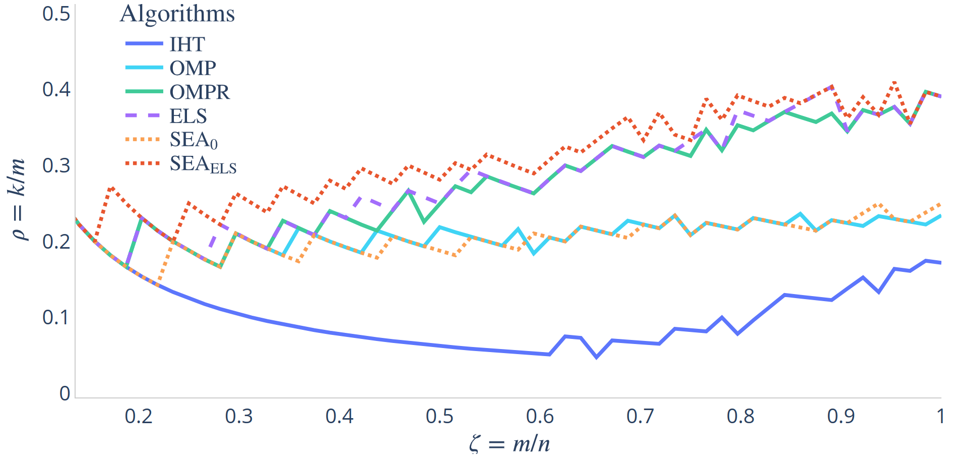
Figure 8: Empirical support recovery phase transition curves in the noisy setup. Problems below each curve are solved by the related algorithm with a success rate larger than $95\%$.

Appendix E Additional results in deconvolution

To supplement Section 4.2, we provide additional results for the initial experimental setup. We provide in Section E.1 the loss along the iterative process for the experiment on Figure 3 in Section 4.2. We also depict in Section E.2 the average of the loss, over the $r=1000$ problems solved to construct Figure 4, when $k$ varies. Finally, we provide results when $e\neq 0_{\mathbb{R}^{m}}$ in Section E.3.

E.1 Deconvolution: The loss along the iterative process

Figure 9 and Figure 10 illustrate the behavior of SEA${}_{\text{0}}$ and SEA${}_{\text{ELS}}$, for the same $6$-sparse $x^{*}$ as Figure 3 in Section 4.2, throughout the iterative process.

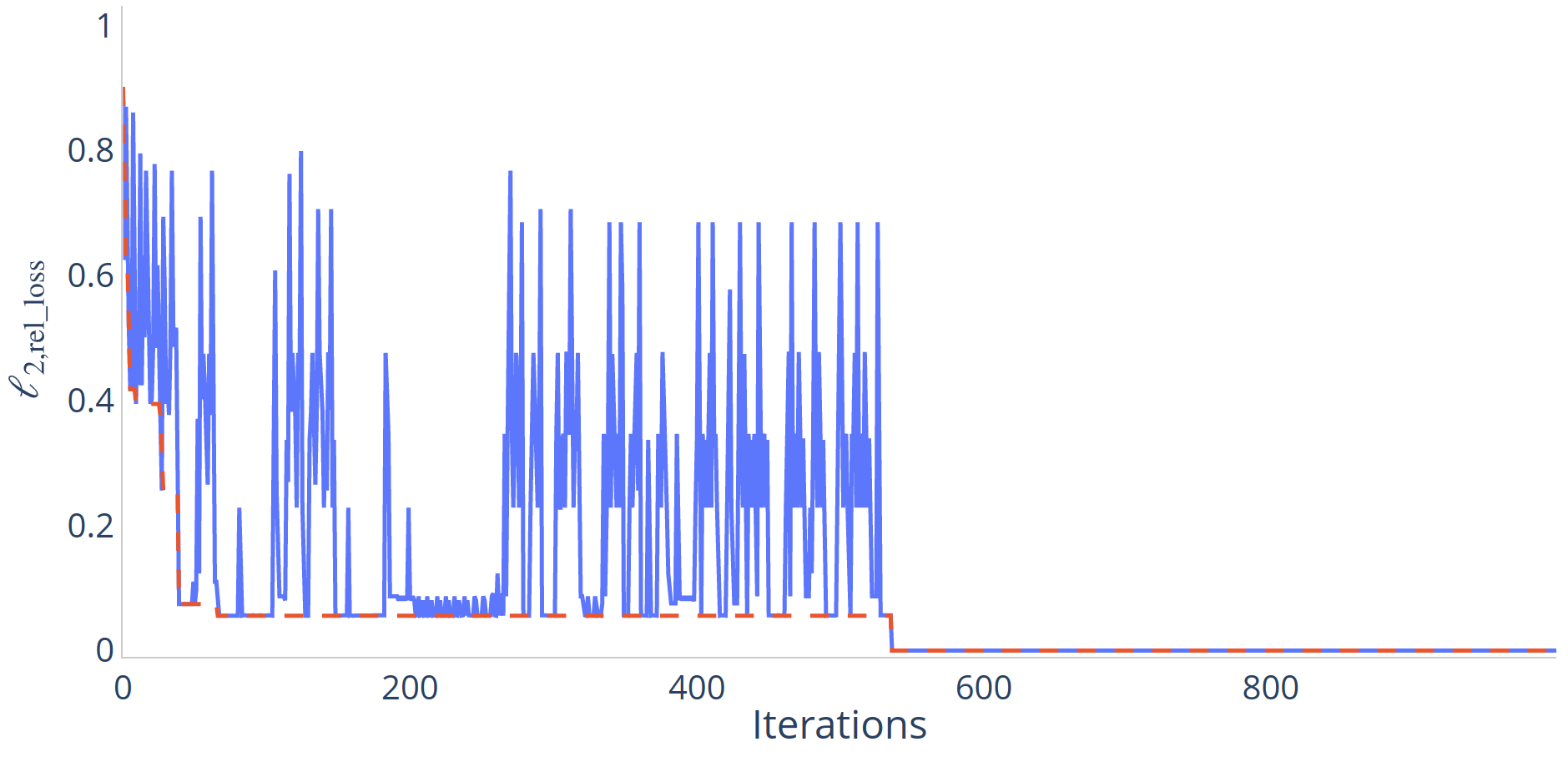
Figure 9: Representation of $\ell_{2,\text{rel}\_\text{loss}}(x^{t})$ (blue) and $\ell_{2,\text{rel}\_\text{loss}}(x^{{t_{BEST}}(t)})$ (dashed red) for each iteration of SEA${}_{\text{0}}$, for the experiment of Figure 3.

More precisely, Figure 9 depicts the results for SEA${}_{\text{0}}$. The blue curve represents $\ell_{2,\text{rel}\_\text{loss}}(x^{t})$ when $t$ varies in $\llbracket 0,1000\rrbracket$, where $\ell_{2,\text{rel}\_\text{loss}}$ is defined by

$$\ell_{2,\text{rel}\_\text{loss}}(x)=\frac{\lVert Ax-y\rVert_{2}}{\lVert y\rVert_{2}}.$$ (38)

The dashed red line represents $\ell_{2,\text{rel}\_\text{loss}}(x^{{t_{BEST}}(t)})$ where ${t_{BEST}}(t)=\underset{{t^{\prime}}\in\llbracket 0,t\rrbracket}{\operatorname{argmin}}\lVert Ax^{t^{\prime}}-y\rVert_{2}^{2}$ and $t$ varies in $\llbracket 0,1000\rrbracket$. Figure 10 illustrates the same results for SEA${}_{\text{ELS}}$. One can observe that, due to the exploratory nature of SEA, $\ell_{2,\text{rel}\_\text{loss}}(x^{t})$ oscillates for both versions of SEA. This does not prevent SEA${}_{\text{0}}$ from finding a good first approximation of $S^{*}$ in the first $80$ iterations and finally recovering $S^{*}$ despite the high coherence of $A$. Once $S^{*}$ is recovered, since the experiment is in a noiseless setting, we have for $t$ sufficiently large $x^{t}=x^{*}$ and therefore $Ax^{t}-y=0$. Using the update rule of $\mathcal{X}^{t}$, line 8 of Algorithm 1, we see that $\mathcal{X}^{t}$ should no longer evolve. This is what we observe on Figure 9.

We observe the same behavior for SEA${}_{\text{ELS}}$, on Figure 10. The exploration recovers $S^{*}$ again. The good initialization permits starting from a better support and recovering $S^{*}$ in fewer iterations though.

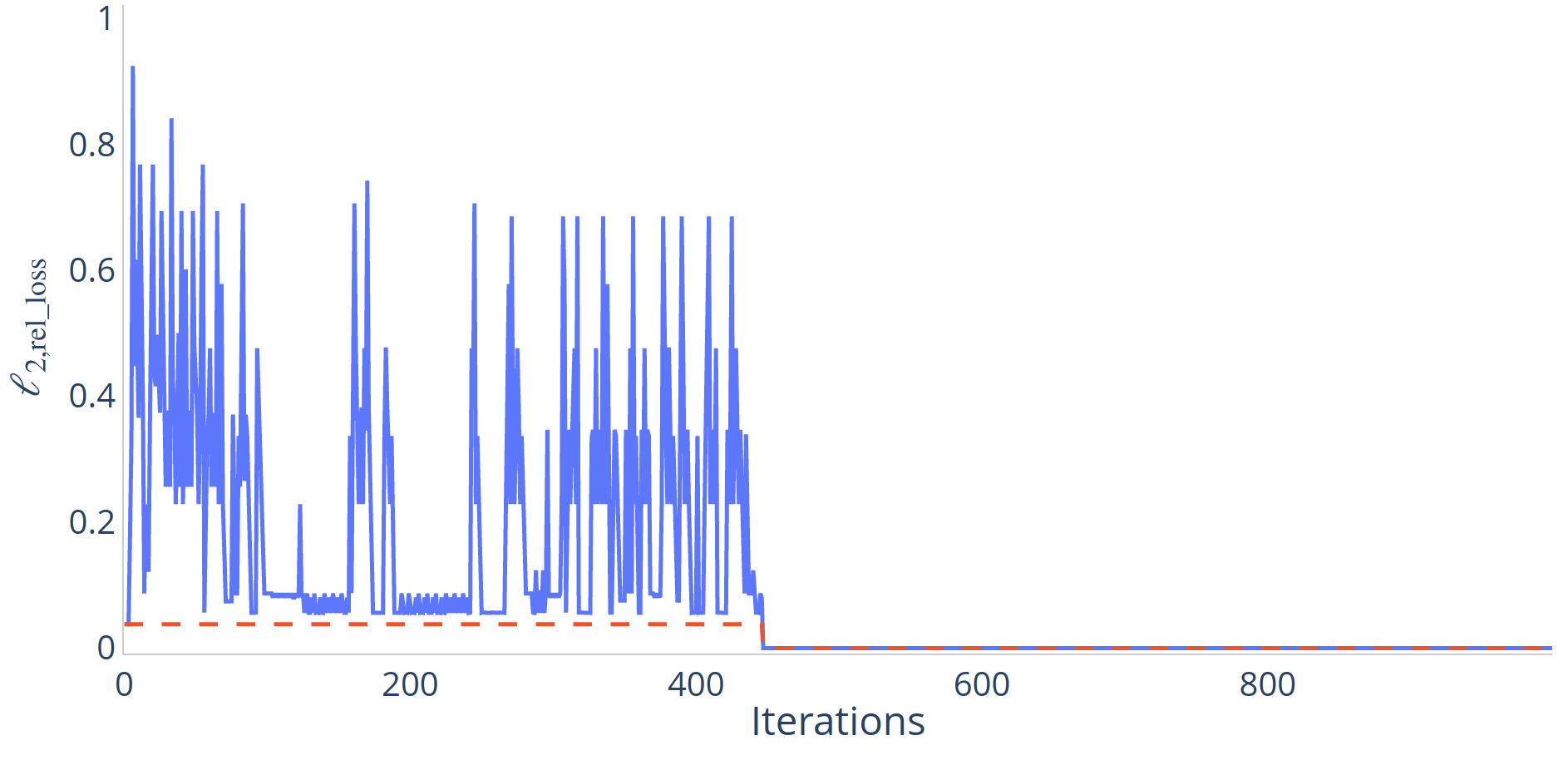
Figure 10: Representation of $\ell_{2,\text{rel}\_\text{loss}}(x^{t})$ (blue) and $\ell_{2,\text{rel}\_\text{loss}}(x^{{t_{BEST}}(t)})$ (dashed red) for each iteration of SEA${}_{\text{ELS}}$, for the experiment of Figure 3.

E.2 Deconvolution: The average loss when $k$ varies

In this section, we consider the experiment described in Section 4.2, whose results are already depicted in Figure 4.

On Figure 11, we show the average – over the $r=1000$ problems – of the relative $\ell_{2}$ loss, defined in (38), for the outputs of all algorithms and for $k\in\llbracket 1,16\rrbracket$. We observe that both versions of SEA reach the same lowest error. The largest gap between SEA and its competitors is reached for $k$ between $2$ and $8$.

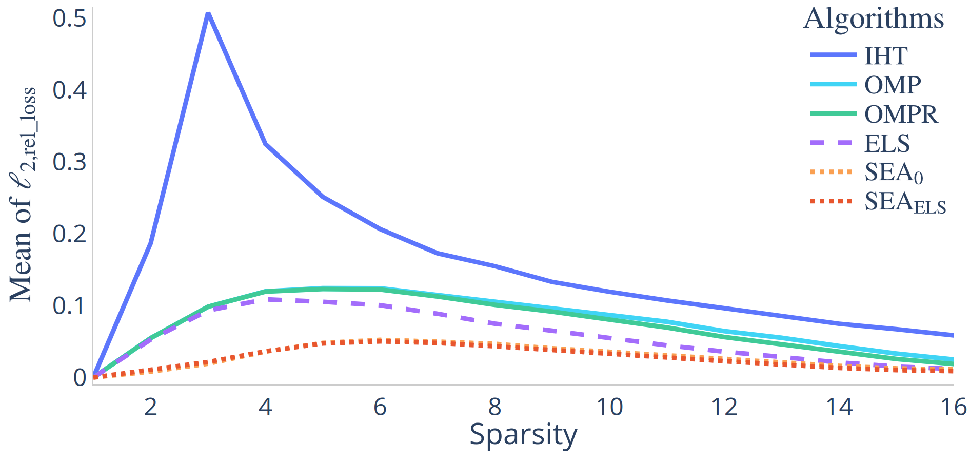
Figure 11: Mean of $\ell_{2,\text{rel}\_\text{loss}}(x)$ for the outputs of the algorithms on the $1000$ problems of Section 4.2, for each sparsity level $k$.

E.3 Deconvolution: Results in the noisy setup

We consider the same experiment as in Section 4.2 but in a noisy setting. The entries of $e$, in (1), are independently drawn from a Gaussian distribution with mean $0$ and standard deviation $0.1$. This leads to an averaged – over $r=1000$ experiments for each $k$ – Signal to Noise Ratio, defined by $\text{SNR}=10\log_{10}(\frac{\lVert x^{*}\rVert_{2}^{2}}{\lVert e\rVert_{2}^{2}})$, ranging from $10$ dB when $k=1$ to $22$ dB when $k=16$.

E.3.1 The loss along the iterative process

The analogues of the curves of Figure 9 and Figure 10 from Section E.1 are respectively in Figure 12 and Figure 13. The conclusions drawn from Figure 12 and Figure 13, in the noisy setting, are similar to the one in Section E.1. Again, initializing SEA with ELS permits SEA${}_{\text{ELS}}$ to find a good approximation of $S^{*}$ in less iterations than SEA${}_{\text{0}}$. However, $\mathcal{X}^{t}$ continues to evolve during all iterations because of the noise that prevents SEA from reaching a zero error.

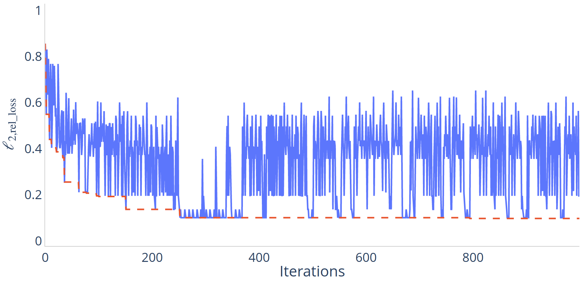
Figure 12: Representation of $\ell_{2,\text{rel}\_\text{loss}}(x^{t})$ (blue) and $\ell_{2,\text{rel}\_\text{loss}}(x^{{t_{BEST}}(t)})$ (dashed red) for each iteration of SEA${}_{\text{0}}$, for the noisy experiment.

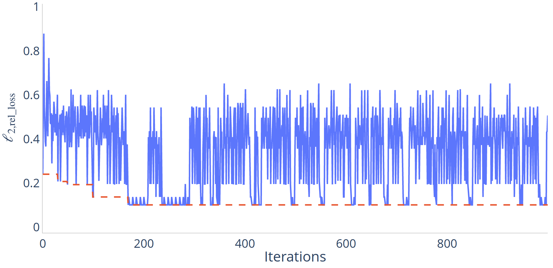
Figure 13: Representation of $\ell_{2,\text{rel}\_\text{loss}}(x^{t})$ (blue) and $\ell_{2,\text{rel}\_\text{loss}}(x^{{t_{BEST}}(t)})$ (dashed red) for each iteration of SEA${}_{\text{ELS}}$, for the noisy experiment.

E.3.2 Observing the losses along with $k$

The analogues of the curves of Figure 4 and Figure 11 are respectively in Figure 14 and Figure 15. Results in the noisy setting are very similar to the ones in Section 4.2 and Section E.2, in the noiseless setting. Figure 14 shows that for sparsity level $k<12$, SEA${}_{\text{0}}$ and SEA${}_{\text{ELS}}$ outperform the other algorithms. Figure 15 shows that because of the noise, optimizing $\ell_{2,\text{rel}\_\text{loss}}$ is harder than in the noiseless setting for all algorithms. However, both versions of SEA still reach the lowest error.

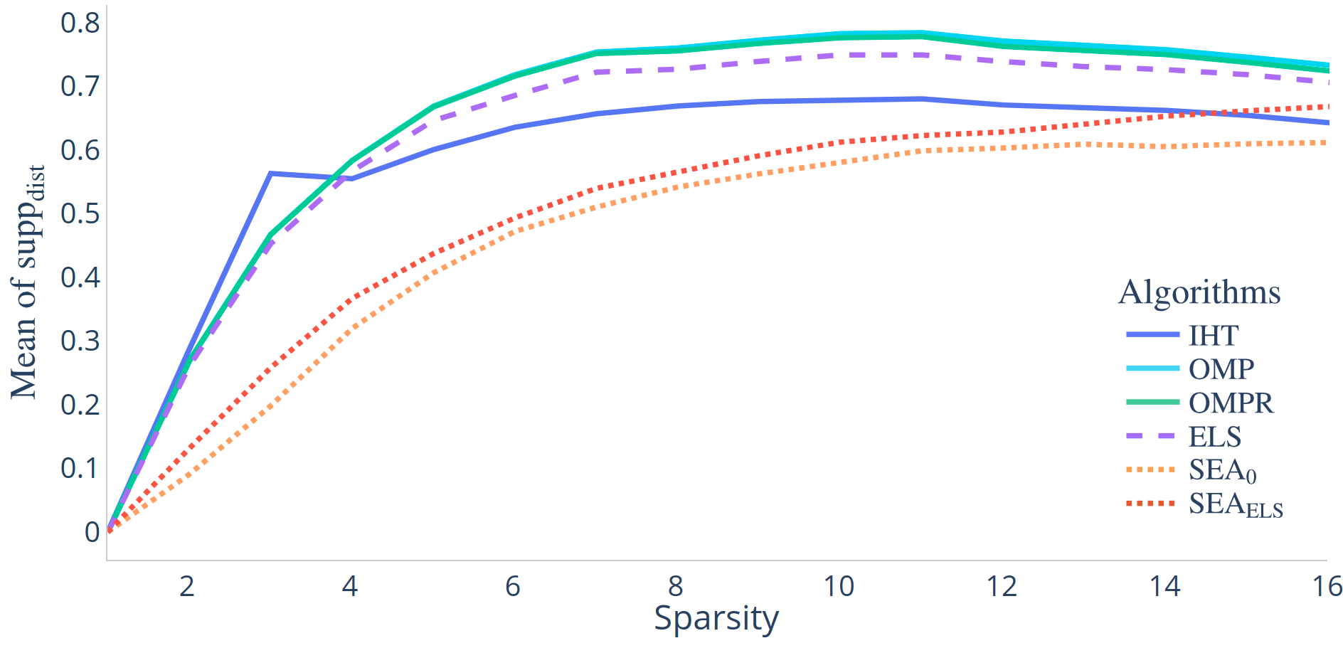
Figure 14: Mean of support distance $\text{supp}_{\text{dist}}$ between $S^{*}$ and the support of the solutions provided by several algorithms as a function of the sparsity level $k$ in the noisy setup.

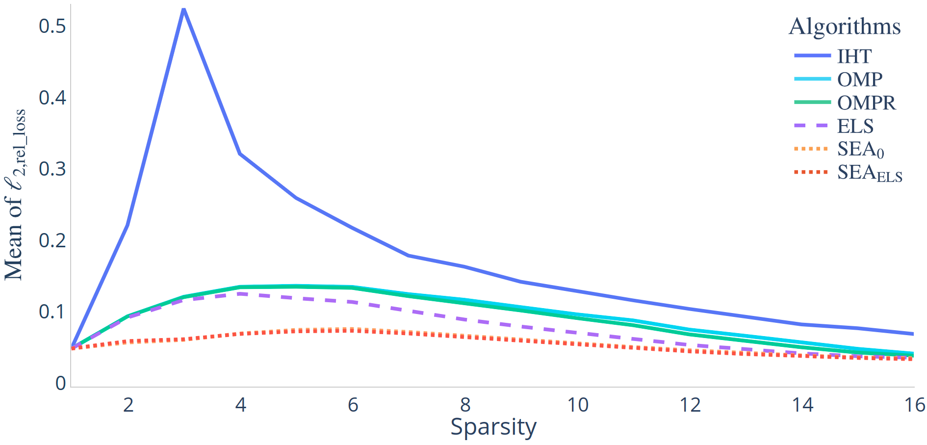
Figure 15: Comparison of the mean of relative $\ell_{2}$ Regression loss $\ell_{2,\text{rel}\_\text{loss}}$ computed for the solutions provided by the algorithms for each sparsity level $k$ in the noisy setup.

Appendix F Additional Machine Learning experiments

To supplement Section 4.3, we provide more experiments on linear and logistic regression. We use the datasets considered in [1]. We present regression problems in Section F.1 and classification problems in Section F.2.

F.1 Regression datasets

The error $\ell_{2}\_\text{loss}(x)=\frac{1}{2}\lVert Ax-y\rVert_{2}^{2}$ is depicted in Figure 16 for the comp-activ-harder dataset ($m=8191$ examples, $n=12$ features), for all $k\in\llbracket 1,12\rrbracket$ and for all algorithms. This is a low-dimensional problem ($n$ is small). We see from this figure that both versions of SEA achieve similar performance to ELS.

The same experiment is reported on Figure 17, but for the dataset slice ($m=53500$ examples, $n=384$ features). This is an intermediate-dimensional problem. Figure 17 shows that SEA${}_{\text{0}}$ obtains slightly worse results than SEA${}_{\text{ELS}}$ and ELS.

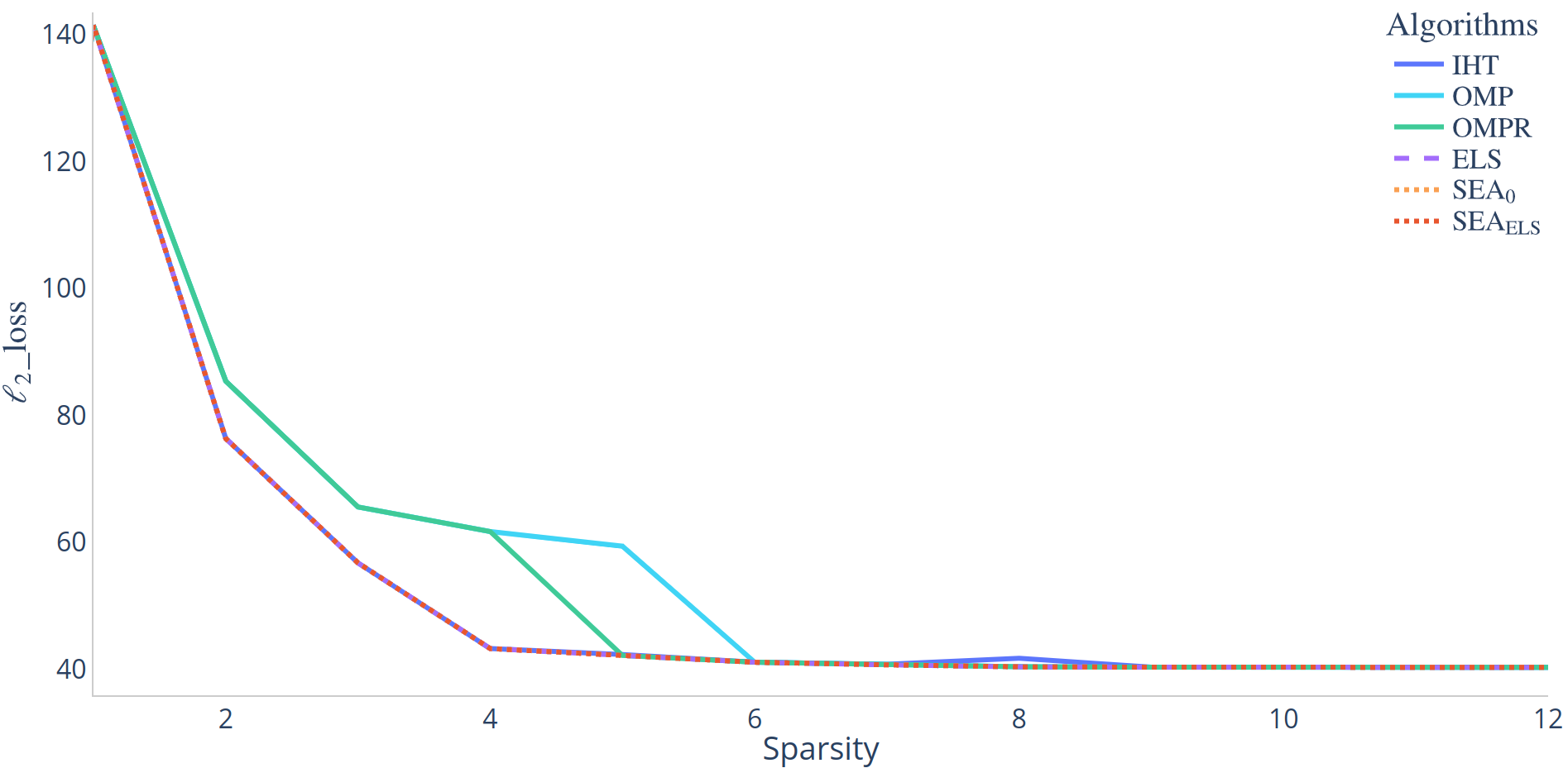
Figure 16: Performance on the regression dataset comp-activ-harder ($m=8191$ examples, $n=12$ features).

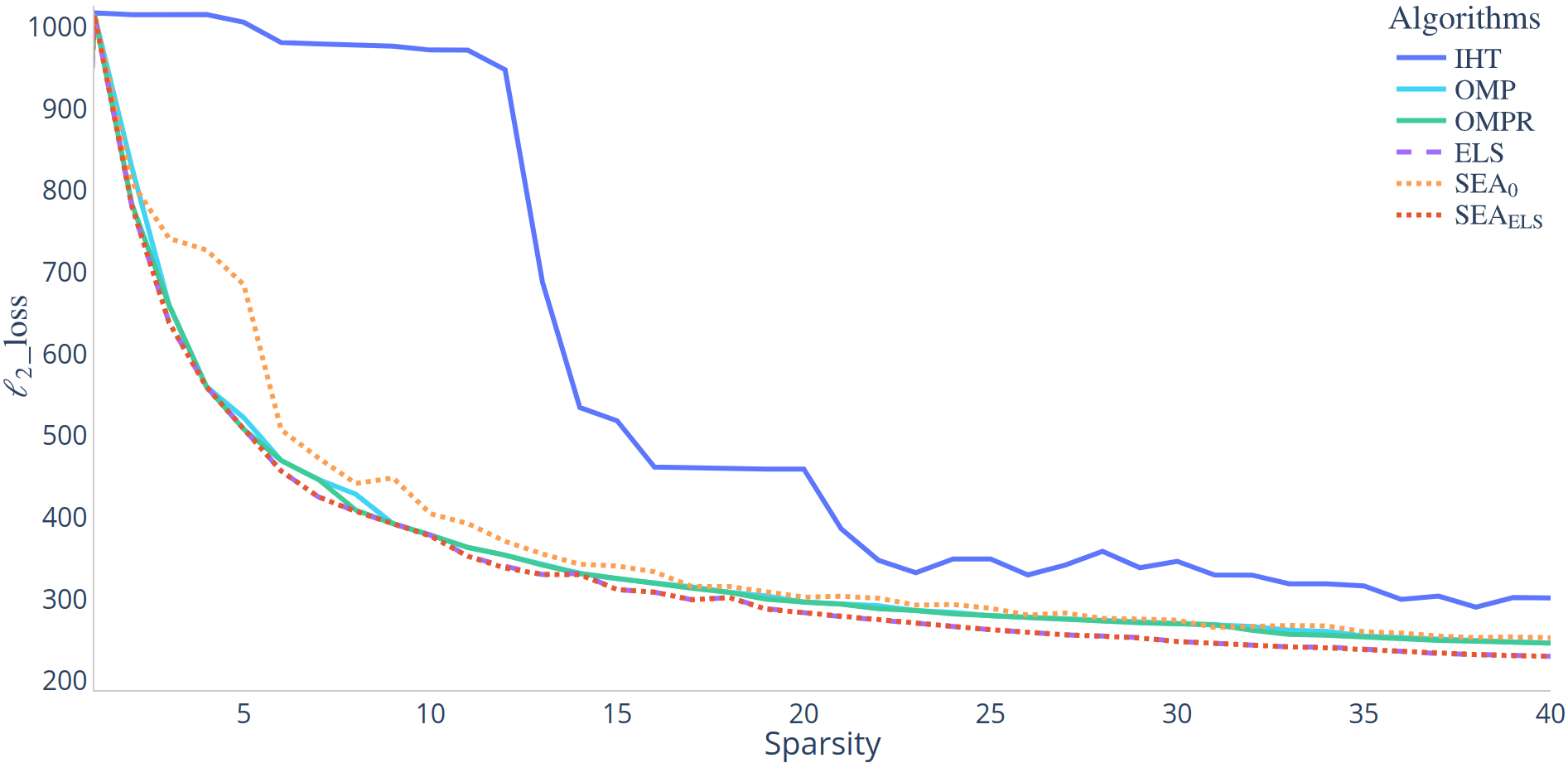
Figure 17: Performance on the regression dataset slice ($m=53500$ examples, $n=384$ features).

F.2 Classification datasets

In these experiments, we consider the logistic regression loss defined by

$$\text{log}\_\text{loss}(x)=\sum_{i=1}^{m}\left(-y_{i}\log(\sigma((Ax)_{i}))-(1-y_{i})\log(1-\sigma((Ax)_{i}))\right),$$

where $\sigma(t)=\frac{1}{1+e^{-t}}$ is the sigmoid function.

We need to adapt SEA to this new loss. In Algorithm 1, line 7 is replaced by $x^{t}=\underset{\begin{subarray}{c}x\in\mathbb{R}^{n}\\ \text{supp}(x)\subset S^{t}\end{subarray}}{\operatorname{argmin}}\text{log}\_\text{loss}(x)$ and line 8 is replaced by $\mathcal{X}^{t+1}=\mathcal{X}^{t}-\eta\nabla\text{log}\_\text{loss}(x^{t})$. Similar adaptations are performed on the other algorithms.

The loss $\text{log}\_\text{loss}(x)$, for the letter dataset ($m=20000$ examples, $n=16$ features), for all $k\in\llbracket 1,12\rrbracket$ and for all algorithms is depicted in Figure 18. We depict the same curves obtained for the ijcnn1 dataset ($m=24995$ examples, $n=22$ features) in Figure 19.

These two last figures show that both SEA${}_{\text{0}}$ and SEA${}_{\text{ELS}}$ achieve similar performances to ELS.

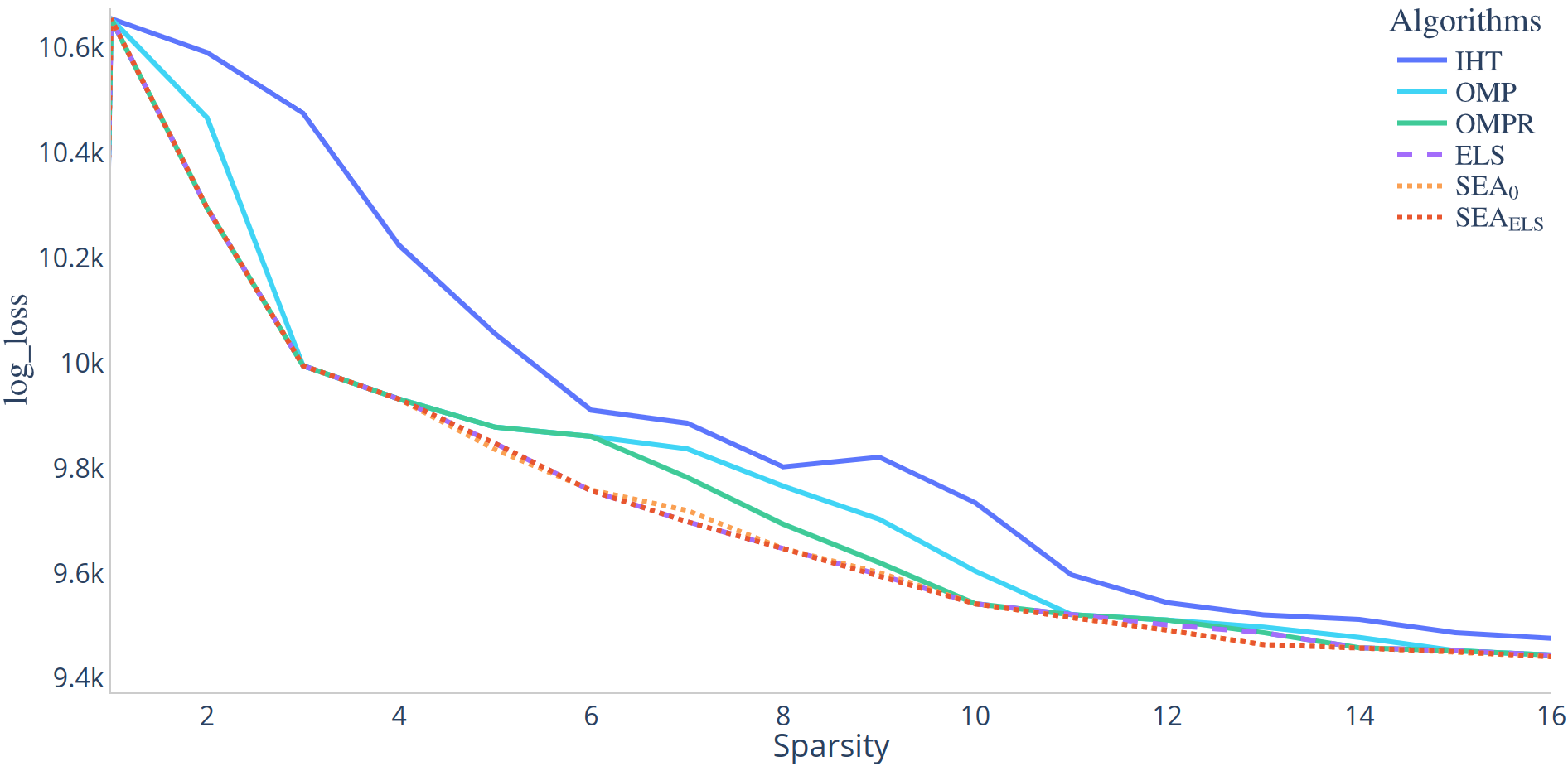
Figure 18: Performance on the classification dataset letter ($m=20000$ examples, $n=16$ features).

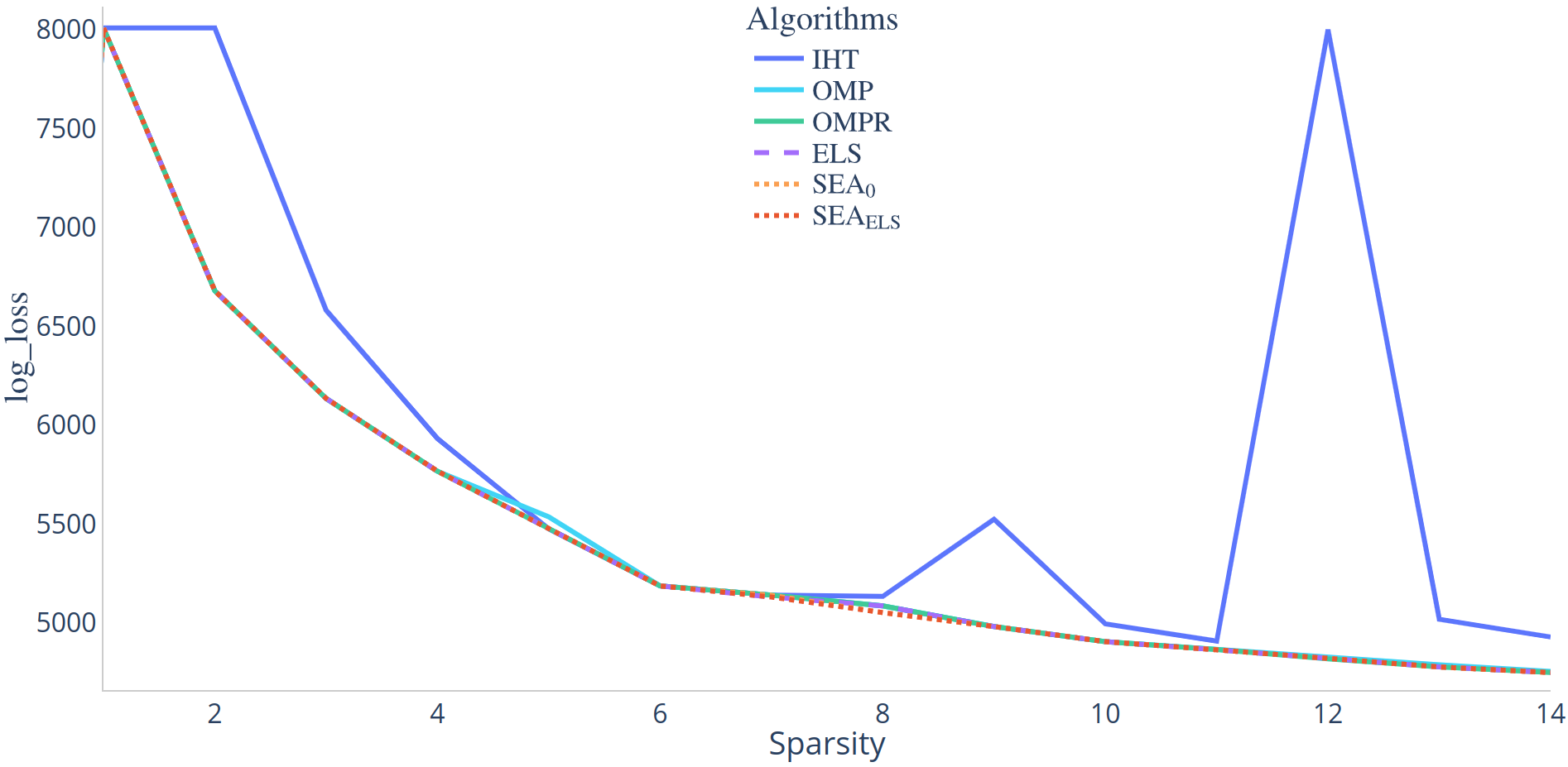
Figure 19: Performance on the classification dataset ijcnn1 ($m=24995$ examples, $n=22$ features).

References

- [1] Kyriakos Axiotis and Maxim Sviridenko. Sparse convex optimization via adaptively regularized hard thresholding. In Proc. Int. Conf. Mach. Learn., volume 119 of Proceedings of Machine Learning Research, pages 452–462. PMLR, 13–18 Jul 2020.
- [2] Bubacarr Bah and Jared Tanner. Bounds of restricted isometry constants in extreme asymptotics: formulae for Gaussian matrices. Lin. Algebra Appl., 441:88–109, 2014.
- [3] Ramzi Ben Mhenni, Sébastien Bourguignon, and Jordan Ninin. Global optimization for sparse solution of least squares problems. Optim. Methods Softw., 37(5):1740–1769, 2022.
- [4] Yoshua Bengio, Nicholas Léonard, and Aaron Courville. Estimating or propagating gradients through stochastic neurons for conditional computation. CoRR, arXiv:1308.3432, 2013.
- [5] Brett Bernstein and Carlos Fernandez-Granda. Deconvolution of point sources: A sampling theorem and robustness guarantees. Comm. Pure Appl. Math., 72(6):1152–1230, 2019.
- [6] Thomas Blumensath and Mike E. Davies. Iterative hard thresholding for compressed sensing. Appl. Comput. Harmon. Analysis, 27(3):265–274, 2009.
- [7] T Tony Cai and Lie Wang. Orthogonal matching pursuit for sparse signal recovery with noise. IEEE Trans. Inform. Theory, 57(7):4680–4688, 2011.
- [8] Emmanuel J Candès, Justin Romberg, and Terence Tao. Robust uncertainty principles: Exact signal reconstruction from highly incomplete frequency information. IEEE Trans. Inform. Theory, 52(2):489–509, 2006.
- [9] Emmanuel J Candes and Terence Tao. Decoding by linear programming. IEEE Trans. Inform. Theory, 51(12):4203–4215, 2005.
- [10] Scott Shaobing Chen, David L Donoho, and Michael A Saunders. Atomic decomposition by basis pursuit. SIAM Rev., 43(1):129–159, 2001.
- [11] Matthieu Courbariaux, Yoshua Bengio, and Jean-Pierre David. Binaryconnect: Training deep neural networks with binary weights during propagations. In Adv. Neural Inf. Process. Syst., volume 28, pages 3123–3131, Montreal, Quebec, Canada, Dec. 7–12 2015.
- [12] Wei Dai and Olgica Milenkovic. Subspace pursuit for compressive sensing signal reconstruction. IEEE Trans. Inform. Theory, 55(5):2230–2249, 2009.
- [13] Geoff Davis, Stephane Mallat, and Marco Avellaneda. Adaptive greedy approximations. Constr. Approx., 13(1):57–98, 1997.
- [14] David Donoho and Jared Tanner. Observed universality of phase transitions in high-dimensional geometry, with implications for modern data analysis and signal processing. Phil. Trans. R. Soc. A, 367(1906):4273–4293, 2009.
- [15] David L Donoho. Compressed sensing. IEEE Trans. Inform. Theory, 52(4):1289–1306, 2006.
- [16] Vincent Duval and Gabriel Peyré. Sparse spikes super-resolution on thin grids I: the LASSO. Inverse Problems, 33(5):055008, 2017.
- [17] Vincent Duval and Gabriel Peyré. Exact support recovery for sparse spikes deconvolution. Found. Comput. Math., 15(5):1315–1355, 2015.
- [18] Michael Elad. Sparse and Redundant Representations. Springer New York, NY, 1 edition, 2010.
- [19] Simon Foucart. Hard thresholding pursuit: an algorithm for compressive sensing. SIAM J. Numer. Anal., 49(6):2543–2563, 2011.
- [20] Trevor Hastie, Robert Tibshirani, and Martin Wainwright. Statistical Learning with Sparsity. Chapman and Hall/CRC, May 2015.
- [21] G. Hinton. Neural networks for machine learning. Coursera, video lectures, 2012. Lecture 15b.
- [22] Itay Hubara, Matthieu Courbariaux, Daniel Soudry, Ran El-Yaniv, and Yoshua Bengio. Binarized neural networks. Adv. Neural Inf. Process. Syst., 29, Dec. 5–10 2016.
- [23] Prateek Jain, Ambuj Tewari, and Inderjit Dhillon. Orthogonal matching pursuit with replacement. Adv. Neural Inf. Process. Syst., 24, Dec. 12–17 2011.
- [24] Han-Wen Kuo, Yenson Lau, Yuqian Zhang, and John Wright. Geometry and symmetry in short-and-sparse deconvolution. In Proc. Int. Conf. Mach. Learn., volume 97 of Proceedings of Machine Learning Research, pages 3570–3580. PMLR, 09–15 Jun 2019.
- [25] Stéphane G Mallat and Zhifeng Zhang. Matching pursuits with time-frequency dictionaries. IEEE Trans. Signal Process., 41(12):3397–3415, 1993.
- [26] Nicolai Meinshausen and Peter Bühlmann. High-dimensional graphs and variable selection with the Lasso. Ann. Statist., 34(3):1436–1462, 2006.
- [27] Deanna Needell and Joel A Tropp. CoSaMP: Iterative signal recovery from incomplete and inaccurate samples. Appl. Comput. Harmon. Analysis, 26(3):301–321, 2009.
- [28] Yagyensh Chandra Pati, Ramin Rezaiifar, and Perinkulam Sambamurthy Krishnaprasad. Orthogonal matching pursuit: Recursive function approximation with applications to wavelet decomposition. In Proc. Asilomar Conf. Signal Syst. Comput., volume 1, pages 40–44, Pacific Grove, CA, USA, 1993. IEEE.
- [29] F. Pedregosa, G. Varoquaux, A. Gramfort, V. Michel, B. Thirion, O. Grisel, M. Blondel, P. Prettenhofer, R. Weiss, V. Dubourg, J. Vanderplas, A. Passos, D. Cournapeau, M. Brucher, M. Perrot, and E. Duchesnay. Scikit-learn: Machine learning in Python. J. Mach. Learn. Res., 12:2825–2830, 2011.
- [30] Shai Shalev-Shwartz, Nathan Srebro, and Tong Zhang. Trading accuracy for sparsity in optimization problems with sparsity constraints. SIAM J. Optim., 20(6):2807–2832, 2010.
- [31] Robert Tibshirani. Regression shrinkage and selection via the lasso. J. R. Stat. Soc. Ser. B Stat. Methodol., 58(1):267–288, 1996.
- [32] Martin J Wainwright. Sharp thresholds for high-dimensional and noisy sparsity recovery using -constrained quadratic programming (Lasso). IEEE Trans. Inform. Theory, 55(5):2183–2202, 2009.
- [33] Xiaotong Yuan, Ping Li, and Tong Zhang. Exact recovery of hard thresholding pursuit. In Adv. Neural Inf. Process. Syst., volume 29, pages 3558–3566, Barcelona, Spain, Dec. 5–10 2016.
- [34] Peng Zhao and Bin Yu. On model selection consistency of Lasso. J. Mach. Learn. Res., 7:2541–2563, 2006.
- [35] Chenzhuo Zhu, Song Han, Huizi Mao, and William J Dally. Trained ternary quantization. In Proc. Int. Conf. Learning Representations, Toulon, France, Apr. 24–26 2017.