Real-time LIDAR localization in natural and urban environments

Abstract

Localization is a key challenge in many robotics applications. In this work we explore LIDAR-based global localization in both urban and natural environments and develop a method suitable for online application. Our approach leverages efficient deep learning architecture capable of learning compact point cloud descriptors directly from 3D data. The method uses an efficient feature space representation of a set of segmented point clouds to match between the current scene and the prior map. We show that down-sampling in the inner layers of the network can significantly reduce computation time without sacrificing performance. We present substantial evaluation of LIDAR-based global localization methods on nine scenarios from six datasets varying between urban, park, forest, and industrial environments. Part of which includes post-processed data from 30 sequences of the Oxford RobotCar dataset, which we make publicly available. Our experiments demonstrate a factor of three reduction of computation, 70% lower memory consumption with marginal loss in localization frequency. The proposed method allows the full pipeline to run on robots with limited computation payload such as drones, quadrupeds, and UGVs as it does not require a GPU at run time.

I INTRODUCTION

Robotic systems are being developed in a large variety of environments. Those environments range from underwater survey [1, 2], aerial inspection [3], indoor autonomy [4], outdoor navigation [5, 6], and natural outdoor exploration [7, 8, 9]. In all of these environments the ability to localize a robot against a prior map of some class is studied as it is one of the most basic and fundamental capabilities in robotics.

In our work we aim to achieve a localization performance which is robust across a broad range of environments. To obtain state-of-the-art performance in varied environments we take advantage of neural network architectures that can learn the most appropriate representation of the environment. In this paper we present an approach that learns features capable of generalizing between multiple environments.

When designing a solution to the localization problem, one needs to address the limited resources available on-board an autonomous robot. In contrast to other fields of engineering or computer science, the robot is mobile and needs to carry its own computation and power resources. For example, [10] and [11] studied the need to co-design a mobile robot’s software and hardware. While deep learning solutions have gained popularity due to their performance, it has been difficult to leverage them on smaller light-weight platforms because they frequently require GPU hardware that consumes large amounts of power. The solutions we aim for should be able to use the power of deep learning approaches while not imposing the need for a GPU on the robot. This has clear advantages as it makes the system more applicable to many different robotics platforms.

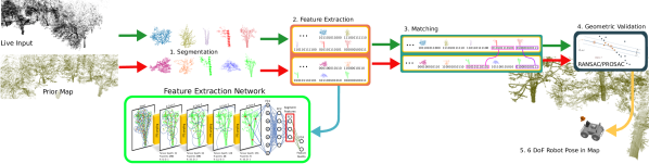
Figure 1: Pipeline outlining our approach to global pose estimation which localizes a live input point cloud within a prior map. The feature extractor network is crucial for enabling efficient CPU performance.

In this paper we present an approach for real-time LIDAR segment-based localization, shown in Fig. 1. This new method is three times faster than the previous best [12] with marginal performance loss. Another contribution of this paper is the creation of rich annotations for LIDAR data for validation involving over $50\,\text{km}$ of testing data and $250\,\text{km}$ of training data. For this, we have aligned and annotated over $2.5$ million point cloud segment matches from the Oxford RobotCar dataset [13]. This substantial effort on improving the dataset will be made available publicly and is one of the biggest LIDAR annotated datasets. We also introduce a second, smaller dataset on which we run field trials on the legged robot ANYmal [14].

In summary, the contributions of our work are as follows:

• We propose a more efficient method for LIDAR localization achieving performance equivalent to state-of-the-art GPU-dependent approaches without the need for heavy computational resources on the robot. By introducing a down-sampled representation in each of the layers in the neural network. The neural network shifts from a representation where all points are maintained throughout the architecture to a novel model that performs down-sampling of the points to limit the computational complexity during inference. This increases the speed of our method by a factor of three and reduces memory consumption by 70%.

• An efficient CPU implementation to solve the Furthest Point Sampling algorithm that achieves a speedup of up to $80$ x, allowing this technique to be applied within the neural network in a CPU in order to handle the efficient down-sampling of the point cloud within the neural network when using only on a CPU.

• We present extensive evaluation of our new approach by comparing to four baselines on six different datasets. In total this represents more than $50\,\text{km}$ of testing data in a variety of environments - park, forest, urban, and industrial scenery. Furthermore, we evaluate the generalization abilities of our approach given different training and testing environments, sensor modalities with different frequency of operation, angular resolution, and mode of operation (2D LIDAR vs 3D LIDAR).

• As a final contribution we offer the community access to the annotated real-world LIDAR dataset. This has been possible by carefully aligning the LIDAR data from 30 different $10\,\text{km}$ trials from the Oxford RobotCar dataset. These trials were collected throughout the whole year. This allows us to retrieve point correspondences between different experiences with a very high degree of accuracy. There are multiple LIDAR samples of the same object, tree or house which is beneficial for supervised neural network training in the presence of appearance change, viewpoint variation, and other challenges.

In the following sections we present the literature relevant to segment-based LIDAR localization. Sec. III describes the proposed network architecture, while Sec. IV describes the used datasets and the proposed improvements of the Aligned Oxford RobotCar dataset. In Sec. V we present extensive evaluation of all LIDAR segment-based methods in terms of feature performance, generalization ability, and computational complexity.

II Related Work

The research presented in this paper focuses on global localization (or loop closure within a SLAM context) using clusters of individual LIDAR segments. This segment-based approach has been shown to be reliable for robot localization [15, 16] and has the advantage of being physically meaningful. In this section the related work will contextualize our approach by describing segment-based approaches using LIDAR data.

A recent approach for global LIDAR localization is to extract small point cloud clusters or segments from the raw input point clouds which are then matched against a prior map and used to localize. A segment is a cluster of LIDAR points broadly but not directly comparable to an object. It might correspond to a patch of a flat wall, a vehicle or a tree trunk. This approach is used instead of determining local keypoints or directly registering the raw points individually.

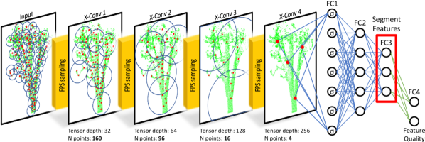
Figure 2: The proposed network architecture. The input to the network is a point cloud segment of 256 points. At each layer the number of points (N), nearest neighbors (K) and dilation rate (D) are specified. The descriptor of the network is extracted from the third fully connected layer (FC3). The architecture also has an additional classification branch (FC4), defining the quality of the descriptor. Between each layer we utilize Farthest Point Sampling (FPS) to efficiently decrease the number of points seen by the network at later stages.

This approach was first proposed by [15] where segments constituted the middle ground between local and global approaches. Global approaches can suffer if they are not robust to occlusions or change in the environment, but they can encapsulate the context of the landmarks/objects present in the scene. Conversely, local methods, similar to the works of [17] and [18], are designed to be robust to occlusions and change, but because they only characterize local regions they lose much of the contextual information. Segments, however, are large enough that they contain reliable and repeatable features while also being robust to occlusions and temporal changes.

Segment localization were first applied to LIDAR localization in the works of [16, 19, 20] and we draw a lot of inspiration from these works. The SegMatch approach extracted more reliable feature matches than the then state-of-the-art 3D point descriptors and could achieve a large number of robust localizations. Similarly to [21], SegMatch’s localizations are obtained by a geometric match pruning of the proposed segments. The centroids of a set of segments are used as input to RANSAC ([22]) which produces the final pose estimate. In [19] segment localization evolved into a segment-based SLAM that introduced a new segment feature that also encoded semantics and volumetric shape. This novel approach learned features from a voxelized input space that were suitable for localization and semantic description of the map. The approach was evaluated in a realistic urban setting and in industrial buildings. In our previous work [23, 12] we proposed a novel descriptor capable of generalizing to natural environments and a new network architecture suitable for CPU operation at test time.

In this work we propose new neural network architecture that performs down-sampling of the point cloud between layers to create a clustering representation within the network instead of per point representation. The main challenge down-sampling within the neural network poses from a computational standpoint is that such a computation can be easily handled with a GPU but requires an efficient CPU implementation that allows it to run in real time, which we describe in this paper. By using this new neural network we can reduce the required computation by a factor of three and occupy 70% less memory at a marginal performance cost.

III METHODOLOGY

The main focus of this work is on global localization where a scene point cloud is matched against a prior map. The localization pipeline is outlined in Fig. 1. In this section we describe our proposed method, named Down-sampled Segment Matching (DSM), which has the following properties: 1) a more efficient neural network architecture for point cloud description suitable for both GPU and CPU inference, and 2) a down-sampled segment descriptor at each layer, which achieves 3) three times quicker inference and 70% less memory utilization than the previous best [12]. The reason for this is that at each layer of the model presented in [12], the $\mathcal{X}$-conv operator [24] computes the k-nearest neighbors for each point, which is very expensive. Here, by carefully sampling the points, we reduce the required computation by a factor of three, while retaining the important information for segment matching. In the following sections we describe the architecture and down-sampling in more detail.

Network Architecture

The architecture for DSM is presented in Figure 2. We have opted for a smaller point size per layer, in order to reduce the computation load in comparison to [12]. The input to our network is a single segment of 256 points. These points are then down-sampled to $160$ in the first layer with the number of nearest neighbours $N=8$. A dilation of $1$ is applied, resulting in the layer processing every point from the input point cloud. Intuitively, our first layer reduces the input by 40%. The second layer of the model has a point size of $96$ with the number of nearest neighbors, $N=10$ and dilation of 2. In this manner we ensure that every point in the new layer is connected to $10$ neighbors from the layer above, which are equally spaced, every 2 points. Therefore, a single point aggregates features in a hierarchical way. Similarly, our third layer has a point size of $16$, each point is connected to $N=12$ neighbors, dilated every $3$ points. This representation shrinks the number of points by 80% with each remaining point being much more informative. The final $\mathcal{X}$-conv layer has size $4$, with $N=16$, and dilation of $1$. This layer ensures that every point in the last layer sees all the possible information, while retaining a small number of points. We have empirically evaluated that this architecture consumes 70% less memory for the same input batch, when compared to our previous work [12], and has slightly fewer parameters ($280$ K compared to $300$ K). We also proposed a different selection methods for points in each subsequent layer including random sampling, inverse density sampling, and Farthest Point Sampling (FPS). Our experiments showed that FPS improves the overall results, as it selects points based on coverage. Using this evidence we established solid grounds on which to propose our novel neural network architecture (DSM) that reduces the computational cost greatly compared to the most computationally efficient baseline [12].

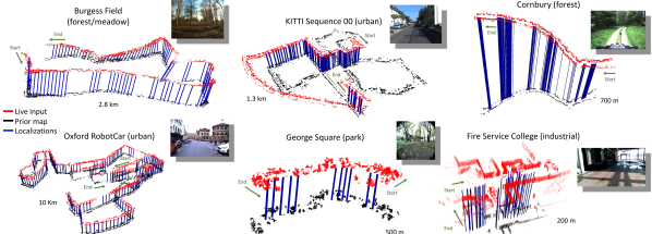
Figure 3: Top-down visual preview of all the datasets considered in our work. The sequence of live point clouds are denoted in red and have been vertically offset from the map clouds (in black) in $Z$ for visualization purposes. The starting and ending poses for each dataset are shown with the indicated green arrows denoting the traversed trajectory. The vertical blue lines indicate a correct place recognition in the map’s reference frame. The length of each dataset and a representative camera image are shown next to each dataset run.

Efficient sampling in compact neural architectures

This section focuses on Farthest Point Sampling (FPS) and describes an efficient implementation of FPS suitable for CPU execution during inference.

The input to the sampling approach are the global $x,y,z$ coordinates of all points, and the number of sampled points required. The first step of the sampling procedure is to select a random point and compute the distance from that point to the rest of the points in the segment. The first point is added to the set of visited points. Thereafter, iteratively the algorithm selects the point that has the biggest distance between its previous point and the rest of the unvisited points and adds it to the list of visited points. This continues until the stopping criteria is reached, i.e the cardinality of the visited set is equal to the input parameter. In this manner the selected points that we convolve are separated as far apart as possible. This helps the convolution retain similar amount of information but with only a small fraction of the points.

This algorithm has been efficiently parallelized using CUDA on a GPU [25]. The authors present results on the effect of randomness when choosing the first point. When training our model we still use the GPU as much as possible as this computation happens offline but for test time we resort to our efficient CPU implementation, which we detail below.

In our work, we wish to utilize sampling in each layer of our architecture while being able to run on a CPU. Initially, we developed our approach to iteratively choose the most distant point in each segment individually. This per-segment approach is not optimal, as it requires $O(PS)$ time complexity, where $P$ denotes the number of segments in a batch, while $S$ – the number of selected points to sample. We improved this by implementing a sampling technique directly on batches of segments in a tensor simultaneously. The data in each layer of our model is structured as a tensor, where the height of the tensor holds each point from the segment, the width corresponds to each of the points’ dimensions (usually $x,y,z$), and the length represents the batch of segments in a point cloud. This way we can efficiently compute the distance matrix of the entire tensor, along the length of the tensor, and simultaneously select the farthest point in all segments.

While the above approach still needs to compute the distance matrix for each following farthest point, it is still more efficient than running on per-segment basis – $O(S)$. In comparison to a per-segment approach, we gain $80$ x speed-up, while compared to the thousands of cores that CUDA utilizes, we are just $30$ x slower, but only using a CPU. By paying attention to the computational details of the sampling, our method operates at a frequency of $5\,\text{Hz}$ on a CPU.

IV Data Structure

A special effort has been made to present broad experimental results for our new method as well as other state-of-the-art segment-based localization methods [16, 19, 23, 12]. To provide the basis of our analysis we used six different datasets, collected using five different platforms in urban, industrial, and natural environments. A top-down view of the localizations at each environment is shown in Fig. 3, while a video preview of our algorithm running on the datasets is available in the supplementary material. Nearly 320 kilometers of data has been analyzed in the results section. We believe that this level of testing is necessary to properly measure and analyze these methods. Of particular note is our large-scale analysis of the RobotCar dataset [13], shown in Fig. 4. As a contribution of this paper we make available an improved version of the dataset by providing refined ground truth poses of its 300 kilometers.

Aligned Oxford RobotCar Dataset

The Oxford RobotCar Dataset contains over 100 sequences of a single consistent route through Oxford, UK, captured over a period of a year on a vehicle equipped with various navigation sensors including a push-broom LIDAR. The dataset contains many different combinations of weather, traffic, and pedestrians. Data were collected in all weather conditions, including heavy rain, night time, direct sunlight, and snow. Road and building works over the period of a year significantly changed sections of the route throughout the full period.

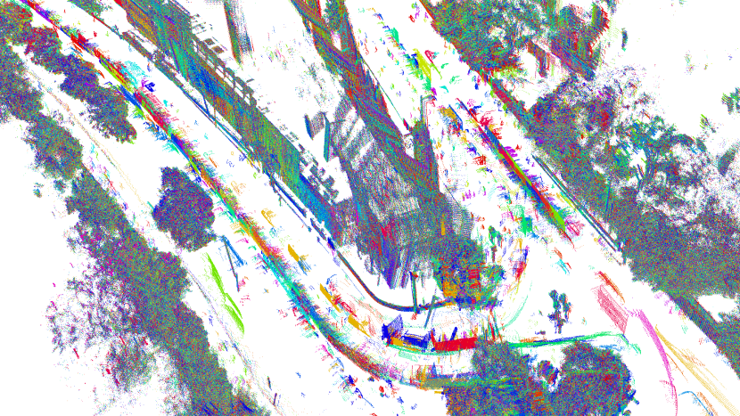
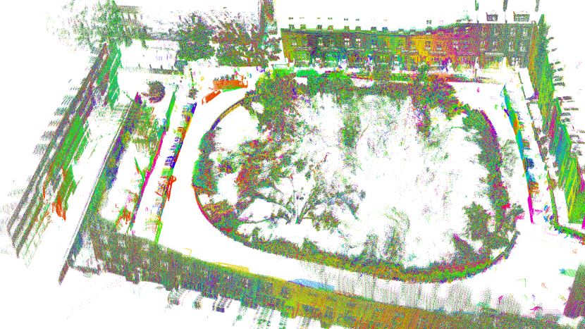
Figure 4: Preview of the aligned Oxford RobotCar dataset across multiple sequences. Each of the 30 point clouds shown in the figure is colored based on the scenario it has been generated from. Parks road junction (left) shows the precise alignment of buildings and vegetation. Wellington Square (right) illustrates a loop around a small park in Oxford, UK.

Ground Truth Annotation

The existing Oxford RobotCar Dataset provides position estimates using a Global Positioning System (GPS) and Inertial Navigation System (INS) which can be used as a proxy for ground truth. However, for deep learning the object instances in the LIDAR data need to be tightly associated to one another. The error due to GPS is in many cases too large to be satisfactory for this. For this reason we employed two months of work annotating a more accurate ground truth. This improved ground truth allowed us to establish correspondences between LIDAR clouds to the accuracy needed for supervised learning. Two example scenes from the aligned dataset are shown in Fig. 4. For a full preview of the improved dataset, please see the videos in the supplementary material.

The ground truth was created as follows: visual odometry provided a backbone with visual loop closures established within and across the 100 sequences [26]. This created an initial map that we then manually corrected by verifying LIDAR consistency and adding individual loop closures where necessary. This provides several samples where each object is seen and allows the feature learning to adapt to viewpoint changes and environment alterations.

Data Organization

In this work we have trained all models and baselines with 26 of the sequences, captured between June 2014 and October 2015, containing a total of 140,287 samples from 59,503 classes. For testing we have used four sequences from November 2015 that were not used during training. We have established 101,502 matching and 2,208,008 non-matching segments. Two segments were considered a match if the distance between their centroids is less than $0.5$ m; and a non-match when the distance is larger than $20$ m. For localization, we generated 3D swathes from the push-broom sensor by incorporating the motion of the vehicle for every $30$ m of distance traveled. This resulted in a total of 1,118 point clouds across all four testing sequences.

We make the ground truth publicly available as a contribution of this paper. It has been added to the same web site as the original dataset. We believe this is very valuable as such a detailed annotation is difficult to attain. We hope it can be useful to other deep learning techniques such as feature learning and change detection.

V RESULTS

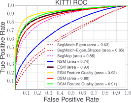
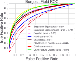
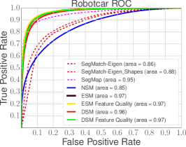
Figure 5: Receiver Operating Characteristic (ROC) curves for the proposed method, DSM, and baseline approaches on KITTI (urban, left), Burgess Field (natural, middle) and Oxford RobotCar (urban, right) datasets.

		SM-Eig		SM-ESF		NSM-RF		SegMap		ESM		ESM-FQ		DSM		DSM-FQ
Test	Train	Area	Perc.	Area	Perc.	Area	Perc.	Area	Perc.	Area	Perc.	Area	Perc.	Area	Perc.	Area	Perc.
	KITTI	0.632	68%	0.655	70%	0.738	79%	0.858	92%	0.902	97%	0.930	100%	0.880	95%	0.911	98%
	Burgess Field	0.666	72%	0.711	76%	0.736	79%	0.764	82%	0.828	89%	0.888	95%	0.864	93%	0.920	99%
KITTI	RobotCar	0.680	73%	0.709	76%	0.752	81%	0.822	88%	0.873	94%	0.890	96%	0.807	87%	0.825	89%
	Burgess Field	0.685	78%	0.714	81%	0.753	85%	0.850	96%	0.836	95%	0.883	100%	0.815	92%	0.869	98%
	KITTI	0.626	71%	0.697	79%	0.713	81%	0.781	88%	0.817	93%	0.868	98%	0.797	90%	0.849	96%
Burgess Field	RobotCar	0.710	80%	0.730	83%	0.732	83%	0.808	92%	0.814	92%	0.853	97%	0.794	90%	0.839	95%
	RobotCar	0.856	88%	0.880	91%	0.848	87%	0.953	98%	0.969	99%	0.972	100%	0.961	99%	0.967	99%
	KITTI	0.760	78%	0.821	84%	0.815	84%	0.952	98%	0.934	96%	0.926	95%	0.928	95%	0.929	96%
RobotCar	Burgess Field	0.819	84%	0.853	88%	0.865	89%	0.951	98%	0.934	96%	0.948	98%	0.922	95%	0.938	97%

TABLE I: Generalization results - difference in performance when training data environment differs from testing data. The best performing algorithm is colored green and the second best orange. Area is the area below the ROC curve, while Perc is the performance relative to the best performing algorithm.

The main focus of this work is to localize a 3D scene point cloud with respect to a prior map. In this section we evaluate the individual components of our system. We also overview several baseline approaches before comparing performance using six challenging datasets.

We compare our method against two popular methods for segment-based localization - SegMatch [16] and the data-driven approach SegMap [19], as well as our previous works - NSM [23] and ESM [12]. When evaluating our experiments we define the following abbreviations (ordered by publication date):

• SM-Eig - SegMatch [16] with only Eigenvalue features.

• SM-ESF - SegMatch [16] using both Eigenvalue and Ensemble of Shape Histogram features (ESF).

• NSM-RF - NSM [23] with Gestalt features and a Random Forest.

• SegMap [19] with voxel-based learning architecture.

• ESM and ESM-FQ[12] - baseline approach with and without a feature quality (FQ) classification branch.

• DSM and DSM-FQ - The proposed method with and without the feature quality of the classification branch.

Due to the modularity of our approach, we can evaluate each component of our system individually and compare it to the baseline methods. First, we examine the effect of the learned features and their performance on three different datasets - two urban scenarios and one parkland scenario. Second, we study the generalization ability of each method by looking at different permutations of training and testing data across the datasets. Third, we address a common issue faced by some approaches relating to rotation variation and viewpoint change. Finally, using the optimal set of system components, we analyze the overall execution of our system in terms of localization performance and runtime efficiency.

Feature Performance

We begin the evaluation by looking at the descriptive power of the features. We chose the KITTI [5], Burgess Field (own), and RobotCar [13] datasets, shown in Fig. 3. We chose these three datasets due to the large amounts of labeled data and the different point cloud density they offer.

To measure performance we compute the Receiver Operating Characteristic (ROC) curve, which measures the true positive rate against the false positive rate for each dataset given a pair of segment descriptors and their labels.

Fig. 5 presents three ROCs for KITTI, Burgess Field, and RobotCar datasets. The proposed method, DSM, is consistently second-best with a difference of 1-2% — but again we emphasize the computational efficiency of DSM. The classification (Feature Quality) branch is trained specifically to provide additional information about whether two point cloud segments match each other. By directly maximizing this metric, the increase in performance of the feature quality branch is evident. We note that all methods perform slightly worse on the natural dataset (Burgess Field) as compared to KITTI, as the trees and bushes in that scene are more challenging to classify. Similarly, all methods perform slightly better on the RobotCar dataset, due to the better alignment and similarity of segments. In line with the literature, we show that learning methods outperform methods based on engineered features [16, 23].

Generalizability

In this section we study the different models to test their ability to generalize to out-of-domain data. We employ the area under the ROC curve (AUC) metric for each permutation of training and testing datasets. We trained our baselines and the proposed model to determine how performance degrades when the testing data domain differs from the training data.

Tab. I presents the AUC for each of the deep learning and Random Forest models. For each testing dataset, the best performing method is indicated with a percentage value of 100% (in green). For ease of reading we compute the loss in performance relative to that best method, expressed again as a percentage (always less than 100%). The second-best method is highlighted in orange.

We note that the Feature Quality branch for the proposed method generalizes much better than the approach without the feature quality classification branch. Regardless of the choice of training and testing dataset, the drop in performance of our model is comparable to the other learning approaches. DSM gives consistently the second best performance, trailing just behind our previous method ESM [12] — with much reduced computation, as we will later see.

When evaluating the hand-crafted feature methods (NSM, SM-Eig, SM-ESF) on the KITTI dataset, we found that Random Forests trained on Oxford RobotCar actually outperform the Random Forest models trained on KITTI. We attribute this to the larger sample size of the Oxford RobotCar dataset and the better alignment of the training data. For the learning approaches, the performance drop is 10% in the worst cases. Interestingly, DSM-FQ, trained on Burgess Field, performs slightly better than when trained on KITTI. We attribute this small variation to the FQ branch of the architecture.

When testing on the Burgess Field dataset, the proposed method (DSM and DSM-FQ) has just a 2% drop of performance when trained on KITTI, and 3% when trained on RobotCar. This is a generalization similar to ESM [12], but better than the other baselines.

On the RobotCar dataset, the trained models of DSM and DSM-FQ consistently perform second best, by about $1\%$ percent — second to ESM [12]. We also note that the scores reported by all algorithms when tested on the RobotCar dataset are consistently higher regardless of the training dataset (inline with the ROC experiment).

In summary, the proposed method, DSM, gives performance which is almost directly comparable to the best performing model with only a 1-2% reduction in performance.

Rotation Variation

So far we showed that deep learning methods perform well when trained and tested on the same datasets, but also generalize well to unseen data. In this section we investigate a common issue in point-based networks, such as the one used in [12]. These types of architectures struggle with viewpoint variation — when the same scene is sensed from different orientations. This is because robustness to this variation is not typically ingrained within the networks.

We train our descriptor, DSM, with rotation augmentation which applies random yaw rotations uniformly sampled between $0$ and $180$ degrees for each sample. We also further pre-process the individual clouds before inputting them to the network. The computational cost associated with this is negligible as we will see later. We chose to compute the following distance as a metric to evaluate how robust our model is to random rotations: $\delta=d(c_{n},c_{0})/Z$, where $d$ is the distance in feature space between a segment $c_{n}$, where $n\in\{0,10,20...360\}$ represents the features of a segment rotated every $10$ degrees and $c_{0}$ (the unrotated reference). $Z$ is a normalization factor that represents the mean distance between all other samples in the dataset. Thus, the metric is lower for architectures that are more robust to rotations.

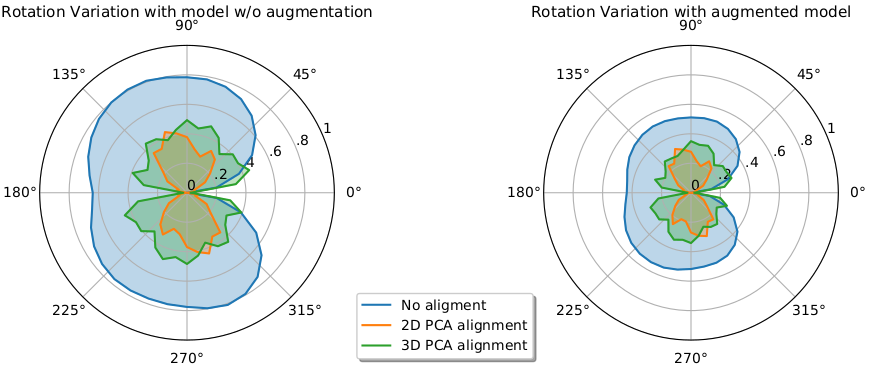
Figure 6: Rotation variation with two models trained without augmentation (left) and with it (right). We have evaluated two alignment strategies based on PCA at different rotation angles. Lower score indicates better performance.

Fig. 6 presents two different variations of our model - with and without applying rotation augmentation to random segments during training, as well as 3 different modes of preprocessing: no preprocessing (similar to [12]), 2D PCA alignment, and 3D PCA alignment. The angle indicates a sample at different rotations ($n$), while the radius value corresponds to $\delta$. The result indicates that while augmentation alleviates the issue, pre-processing is essential for mitigating rotation variations. In experiments which follow we utilize 2D PCA alignment preprocessing.

Test Set Characteristics						Number of Localizations
Name	Type	Length	Sensor	Num. Clouds		SegMatch	NSM	SegMap	ESM	DSM
Oxford RobotCar	Urban	50310 m	Push-broom	1118		80	346	915	896	773
KITTI	Urban	1300 m	Velodyne-HDL-64E	134		41	53	62	63	62
Fire Service College	Industrial	190 m	Velodyne-VLP-16E	169		13	12	35	45	46
George Square	City Park	500 m	Push-broom	30		8	9	8	11	10
Cornbury Forest	Forest	700 m	Velodyne-HDL-32E	1125		N/A	29	231	248	208
Burgess Field	Forest	2800 m	Push-broom	130		41	54	95	94	90

TABLE II: Number of localizations across all datasets.

CPU Multi-core execution times
Algorithm	Desc. size [dim]		Segmentation [ms]	Preprocessing [ms]	Descriptor [ms]	Matching [ms] (K)	Prunning [ms] (RF)	Pose Est. [ms]	Total [ms]
SegMatch	7 (647)		17	0	605	50 (200)	755	64	1491
NSM	66		17	0	24	207 (200)	913	65	1226
SegMap	64		17	15	5902	19 (25)	0	21	5974
ESM	16		17	3	578	8 (25)	0	9	615
DSM	16		17	8	184	8 (25)	0	9	226
CPU Single-core execution times
Algorithm	Desc. size [dim]		Segmentation [ms]	Preprocessing [ms]	Descriptor [ms]	Matching [ms] (K)	Prunning [ms] (RF)	Pose Est. [ms]	Total [ms]
SegMatch	7 (647)		21	0	596	70 (200)	773	64	1524
NSM	66		21	0	37	213 (200)	936	65	1272
SegMap	64		21	26	25945	26 (25)	0	21	26039
ESM	16		21	3	2126	12 (25)	0	11	2173
DSM	16		21	8	731	12 (25)	0	11	783
GPU Computation comparison
Algorithm	Desc. size [dim]		Segmentation [ms]	Preprocessing[ms]	Descriptor [ms]	Matching [ms] (K)	Prunning [ms] (RF)	Pose Est. [ms]	Total [ms]
SegMap	64		17	15	15	19 (25)	0	15	81
ESM	16		17	3	2	8 (25)	0	6	36
DSM	16		17	8	2	8 (25)	0	6	41

TABLE III: Average computation times in milliseconds recorded per point cloud for a localization query on the Burgess Field dataset.

Localization Results

Thus far we have focused primarily on the deep learning part of our approach. In this section we evaluate the complete performance of our method — how well and how often it localizes the current scene within a large prior map.

First, we evaluated an urban environment, consisting of four sequences from the RobotCar dataset and sequence 00 from KITTI. Second, we have considered different types of natural environments: parkland (George Square), forested meadows (Burgess Field), and a heavy forest (Cornbury Forest) — shown in Fig. 3. Third, we tested the algorithms in an industrial setting using the ANYmal quadruped at the Fire Service College, Gloucestershire. These datasets not only present different environments, but also different sensor variations. When evaluating the datasets, it should be noted that the total number of clouds does not reflect the number of possible localizations. This is due to the fact the robots sometimes traversed parts of the environments missing from the prior map. Given this, we were pleased that the approaches are robust and did not compute any false localizations in those areas. For the vegetated datasets, and the industrial dataset we used the model trained on the Burgess Field dataset. Therefore, the training and testing data is inherently different as it comes from different sensors. The rest of the datasets used their corresponding training data - RobotCar trained on another 26 sequences, and KITTI trained on Sequences 05 and 06.

Tab. II shows the localization results for all the datasets. The proposed method performs commensurately to the other learning approaches — ESM [12] and SegMap [19]. Qualitative examples of the performance of our algorithms is illustrated in Figure 3 and the video in the supplementary material. The supplementary material also shows the proposed algorithm evaluated on the Newer College dataset [27].

Computational Efficiency

To this end we demonstrated the performance of our method, in this section we study the computational cost associated with each method.

We tested the methods on a mobile Intel Xeon E3-1535M CPU with the following configurations: 1) a single-core, 2) multi-cores of the same processor, and 3) the CPU with a NVIDIA Titan Xp GPU. We have processed the push-broom point clouds from Burgess Field and recorded the mean computation time as milliseconds per localization query.

To provide a fair comparison, we have used the same Euclidean segmentation for the approaches to create the same segments, and thus the segmentation time is equivalent. We empirically evaluated the number of neighbors in feature space ($K$) to retrieve the most positive localizations, while keeping zero false positives - $25$ for learned approaches, and $200$ for hand-engineered ones. The value of $K$ influences the pose estimation stage as well. We also note that the descriptor size affects the time for matching and pruning.

Tab. III summarizes the recorded GPU and CPU times for all the approaches. The proposed method, DSM, performs three times faster than the previous best [12] on a CPU, while performing similarly on a GPU. We attribute this to the sampling performed at each layer, as the number of parameters is fairly similar between the two architectures - $280$ K vs $300$ K. We also note that the cost of preprocessing using PCA alignment is negligible compared to the other components and is justified given the benefits we saw from the Rotation Variation experiment. When training DSM we noticed that the GPU memory consumption compared to ESM [12] for the same batch size was 70% less. Therefore, to fully utilize the GPU we have increased the batch size when training DSM. We also note that the pose estimator computes a transformation estimate quicker, due to the probability information extracted from the classification branch and the use of the PROSAC estimator [28].

VI CONCLUSION

In this paper we discussed the problem of place recognition based on LIDAR segment matching in both urban and natural environments. Our newly proposed method (DSM) works at three times the frequency of our previous best, while requiring only a CPU. We showed that by down-sampling in the inner layers of the architecture, we gain this significant computation cost reduction. We presented an efficient CPU implementation of the FPS algorithm and we also addressed a common issue with rotation variation through experimental comparison and data augmentation. We have thoroughly validated our methodology on nine scenarios from six different datasets in various environments. Finally, a significant contribution to the Oxford RobotCar dataset was made, and is being made available to the community through this paper, with improved alignment and ground truth labeling. We hope that the robotics community will adopt this dataset for more learning tasks.

References

- [1] M. Miller, S.-J. Chung, and S. Hutchinson, “The Visual–inertial canoe dataset,” IJRR, vol. 37, no. 1, pp. 13–20, 2018.
- [2] L. Paull, M. Seto, J. J. Leonard, and H. Li, “Probabilistic cooperative mobile robot area coverage and its application to autonomous seabed mapping,” IJRR, vol. 37, no. 1, pp. 21–45, 2018.
- [3] H. Goforth and S. Lucey, “GPS-Denied UAV Localization using Pre-existing Satellite Imagery,” in ICRA, May 2019, pp. 2974–2980.
- [4] J. Martínez-Gómez, I. García-Varea, M. Cazorla, and V. Morell, “ViDRILO: The visual and depth robot indoor localization with objects information dataset,” IJRR, vol. 34, no. 14, pp. 1681–1687, 2015.
- [5] A. Geiger, P. Lenz, C. Stiller, and R. Urtasun, “Vision meets robotics: The KITTI dataset,” IJRR, vol. 32, no. 11, pp. 1231–1237, 2013.
- [6] J.-L. Blanco-Claraco, F. Ángel Moreno-Dueñas, and J. González-Jiménez, “The málaga urban dataset: High-rate stereo and lidar in a realistic urban scenario,” IJRR, vol. 33, no. 2, pp. 207–214, 2014.
- [7] T. Pire, M. Mujica, J. Civera, and E. Kofman, “The rosario dataset: Multisensor data for localization and mapping in agricultural environments,” IJRR, vol. 38, no. 6, pp. 633–641, 2019.
- [8] J. P. Underwood, G. Jagbrant, J. I. Nieto, and S. Sukkarieh, “LIDAR-based tree recognition and platform localization in orchards,” JFR, vol. 32, no. 8, pp. 1056–1074, 2015.
- [9] J. Garforth and B. Webb, “Visual appearance analysis of forest scenes for monocular SLAM,” in ICRA, May 2019, pp. 1794–1800.
- [10] F. Ma, L. Carlone, U. Ayaz, and S. Karaman, “Sparse sensing for resource-constrained depth reconstruction,” in IROS, Oct 2016, pp. 96–103.
- [11] J. L. S. Rincon, P. Tokekar, V. Kumar, and S. Carpin, “Rapid deployment of mobile robots under temporal, performance, perception, and resource constraints,” RAL, vol. 2, no. 4, pp. 2016–2023, Oct 2017.
- [12] G. Tinchev, A. Penate-Sanchez, and M. Fallon, “Learning to see the wood for the trees: Deep laser localization in urban and natural environments on a CPU,” in ICRA, May 2019, pp. 1327–1334.
- [13] W. Maddern, G. Pascoe, C. Linegar, and P. Newman, “1 Year, 1000km: The Oxford RobotCar Dataset,” IJRR, vol. 36, no. 1, pp. 3–15, 2017.
- [14] M. Hutter, C. Gehring, A. Lauber, F. Gunther, C. D. Bellicoso, V. Tsounis, P. Fankhauser, R. Diethelm, S. Bachmann, M. Blösch, H. Kolvenbach, M. Bjelonic, L. Isler, and K. Meyer, “ANYmal - toward legged robots for harsh environments,” AURO, vol. 31, no. 17, pp. 918 – 931, 2017.
- [15] B. Douillard, A. Quadros, P. Morton, J. P. Underwood, M. D. Deuge, S. Hugosson, M. Hallström, and T. Bailey, “Scan segments matching for pairwise 3D alignment,” in ICRA, May 2012, pp. 3033–3040.
- [16] R. Dubé, D. Dugas, E. Stumm, J. Nieto, R. Siegwart, and C. C. Lerma, “SegMatch: Segment based place recognition in 3D point clouds,” in ICRA, 2017, pp. 5266–5272.
- [17] Y. Zhuang, N. Jiang, H. Hu, and F. Yan, “3-D-laser-based scene measurement and place recognition for mobile robots in dynamic indoor environments,” TIM, vol. 62, no. 2, pp. 438–450, 2012.
- [18] B. Steder, M. Ruhnke, S. Grzonka, and W. Burgard, “Place recognition in 3D scans using a combination of bag of words and point feature based relative pose estimation,” in IROS. IEEE, 2011, pp. 1249–1255.
- [19] R. Dubé, A. Cramariuc, D. Dugas, J. Nieto, R. Siegwart, and C. Cadena, “SegMap: 3D Segment Mapping using Data-Driven Descriptors,” in RSS, Pittsburgh, Pennsylvania, Jun 2018, pp. 20–30.
- [20] R. Dubé, A. Cramariuc, D. Dugas, H. Sommer, M. Dymczyk, J. Nieto, R. Siegwart, and C. Cadena, “SegMap: Segment-based mapping and localization using data-driven descriptors,” IJRR, vol. 0, no. 0, 2019.
- [21] C. Zach, A. Penate-Sanchez, and M.-T. Pham, “A dynamic programming approach for fast and robust object pose recognition from range images,” in CVPR, 2015, pp. 196–203.
- [22] M. A. Fischler and R. C. Bolles, “Random sample consensus: a paradigm for model fitting with applications to image analysis and automated cartography,” CACM, vol. 24, no. 6, pp. 381–395, 1981.
- [23] G. Tinchev, S. Nobili, and M. Fallon, “Seeing the Wood for the Trees: Reliable Localization in Urban and Natural Environments,” in IROS, 2018, pp. 8239–8246.
- [24] Y. Li, R. Bu, M. Sun, and B. Chen, “PointCNN,” arXiv preprint arXiv:1801.07791, 2018.
- [25] C. R. Qi, L. Yi, H. Su, and L. J. Guibas, “PointNet++: Deep Hierarchical Feature Learning on Point Sets in a Metric Space,” in NIPS, 2017, pp. 5099–5108.
- [26] W. Churchill and P. Newman, “Experience-based Navigation for Long-term Localisation,” IJRR, 2013.
- [27] M. Ramezani, Y. Wang, M. Camurri, D. Wisth, M. Mattamala, and M. Fallon, “The newer college dataset: Handheld LiDAR, inertial and vision with ground truth,” in IROS, 2020.
- [28] O. Chum and J. Matas, “Matching with PROSAC - progressive sample consensus,” in CVPR, 2005, pp. 220–226.