Recurrences reveal shared causal drivers of complex time series

Abstract

Many experimental time series measurements share unobserved causal drivers. Examples include genes targeted by transcription factors, ocean flows influenced by large-scale atmospheric currents, and motor circuits steered by descending neurons. Reliably inferring this unseen driving force is necessary to understand the intermittent nature of top-down control schemes in diverse biological and engineered systems. Here, we introduce a new unsupervised learning algorithm that uses recurrences in time series measurements to gradually reconstruct an unobserved driving signal. Drawing on the mathematical theory of skew-product dynamical systems, we identify recurrence events shared across response time series, which implicitly define a recurrence graph with glass-like structure. As the amount or quality of observed data improves, this recurrence graph undergoes a percolation transition manifesting as weak ergodicity breaking for random walks on the induced landscape—revealing the shared driver’s dynamics, even in the presence of strongly corrupted or noisy measurements. Across several thousand random dynamical systems, we empirically quantify the dependence of reconstruction accuracy on the rate of information transfer from a chaotic driver to the response systems, and we find that effective reconstruction proceeds through gradual approximation of the driver’s dominant orbit topology. Through extensive benchmarks against classical and neural-network-based signal processing techniques, we demonstrate our method’s strong ability to extract causal driving signals from diverse real-world datasets spanning ecology, genomics, fluid dynamics, and physiology.

I Introduction

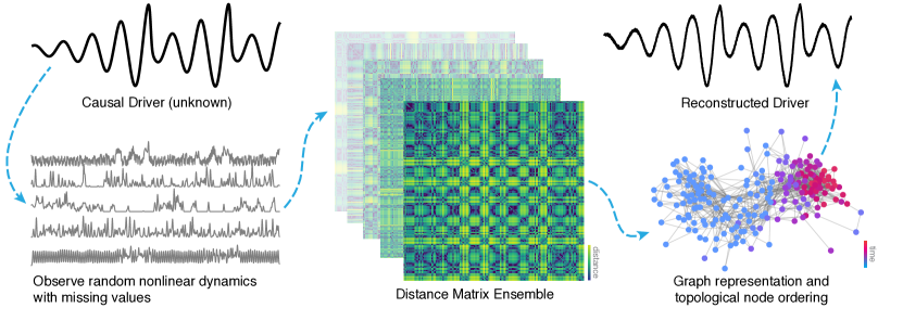
Figure 1: An example application of the shared dynamics reconstruction method. An unobserved driver influences an ensemble of dynamical systems, which each contain unique internal dynamics and random measurement filters. Here, we use the Rössler dynamical system to drive an ensemble of Lorenz systems with random parameters that have been filtered with random Gaussian response functions. Timepoint-wise recurrence graphs are separately calculated for each response, and then aggregated to produce a consensus adjacency graph. This graph is traversed and sorted using a diffusion process, the longest transient of which reconstructs the driver dynamics.

Diverse biological and engineered systems exhibit descending control, in which a central driving signal causally influences the state of multiple response variables—which cannot, in turn, influence the driver. In ecological food webs, environmental changes trigger complex cascades of trophic interactions [1], while in animal nervous systems, descending neurons convey cognitive imperatives to motor circuits that implement behavior [2]. In systems biology, master regulators such as the Hox gene family orchestrate numerous complex gene regulatory networks during development [3]. The ubiquity of top-down control may arise from the robustness and parsimony it confers relative to the number of dynamical interactions [4]; however, it also introduces experimental challenges when the driving variable is not known a priori, or is not directly observable.

From a computational perspective, the driving signal encodes information about itself into the states of the responding subsystems. The coupling between the driver and responses acts as a lossy transmission channel—motivating recent methods for detection of causal interactions based on mutual information and transfer entropy [5, 6, 7, 8]. Alternatively, causal relationships can be inferred based on properties of the dynamical system that generates a time series: theorems from nonlinear dynamics suggest that partial information present in observable subsystems can reveal subregimes within the driving signal [9], motivating recent methods that determine causality based on attractor reconstruction or unsupervised learning of latent representations [10, 11, 12, 13, 14], which draw inspiration from classical results regarding the observability of dynamical systems [15, 16, 17].

However, while many existing methods detect the average strength and directionality of causal interactions among known variables, resolving their temporal dynamics has received less attention. Yet understanding how causal forces change over time is necessary to understand control schemes, particularly in biological systems in which control signals are sparse and infrequent [18]. Time-resolved driving signals may be detected based on signal denoising or assimilation techniques, or by generalizing statistical causality measures using time-dependent kernels [9, 19, 20]. However, these methods fail to leverage existing theoretical works on skew-product dynamical systems and chaotic synchronization [21, 22, 23], which provide a strong inductive bias that may help obtain robust, physically-motivated representations even from highly corrupted measurements.

Here, we introduce a general unsupervised learning method that reconstructs an unobserved driver time series, given many partial or noisy observations of response time series. Based on the intuition that recurrences in response systems imply recurrences in the driver state, we traverse a network representation of the observed time series in order to identify unique driver states, allowing our method to identify temporal progressions of driver states even from highly nonlinear or noisy response measurements. Our method applies to both discrete- and continuous-time signals with either oscillatory or aperiodic driving, and we show that its underlying accuracy corresponds to structural properties of the observed time series in the form of an ergodicity-breaking percolation transition in the time series adjacency graph. We extensively compare our technique against existing methods based on mutual information, artificial neural networks, and spectral transformations, and obtain strong results on diverse datasets spanning electrophysiology, hydrodynamics, and systems biology. Moreover, we find that our method’s accuracy arises from its ability to identify and approximate unstable periodic orbits that the driving signal transiently shadows—linking our algorithm’s performance to topological properties of the underlying systems.

II Approach

II.1 Recurrence structure of skew-product causal systems

Suppose an unknown signal $\mathbf{z}(t)$ drives $N$ response dynamical systems $\dot{\mathbf{y}}_{k}(t)=\mathbf{g}_{k}(\mathbf{z}(t),\mathbf{y}_{k}(t),t)$, $k\in\{1,2,...,N\}$. Given a set of response signals $\{\mathbf{x}_{k}(t)\}_{N}$ comprising nonlinear measurements $\mathbf{x}_{k}(t)=\mathcal{M}_{k}\circ\mathbf{y}_{k}(t)$ we seek a reconstruction of the original driver $\hat{\mathbf{z}}(t)$. In principle, this problem is underdetermined, because the measurement operator $\mathcal{M}_{k}$ may be noninvertible, or the internal dynamics of each response variable $\mathbf{y}_{k}$ may only very weakly couple to the driving signal.

However, if the driver state lies on an attractor $\mathcal{Z}$, while the $k^{th}$ response signal lies on an attractor $\mathcal{Y}_{k}$, then the overall dynamics have skew product structure with combined attractor $\mathcal{Z}\times\mathcal{Y}_{1}\times\mathcal{Y}_{2}\times...\times\mathcal{Y}_{N}$. While individual $\mathcal{Y}_{k}$ are not directly observable, the skew product reconstruction theorem of Stark suggests that a one-to-one mapping $\hat{\mathcal{Y}}_{k}\sim\mathcal{Y}_{k}$ may be constructed from the observed signal $\mathbf{x}_{k}(t)$ by applying a lift $\phi(.)$ to the signal using time delays $\hat{\mathbf{y}}_{k}(t)=\phi(\mathbf{x}_{k}(t))=[\mathbf{x}_{k}(t),\mathbf{x}_{k}(t-\tau),\mathbf{x}_{k}(t-2\tau),...,\mathbf{x}_{k}(t-(D-1)\tau)]^{\top}$, where $D$ and $\tau$ are hyperparameters chosen using a variety of heuristics [15, 16, 17]. Nonlinear generalizations of the lifting map $\phi$ may be obtained with attractor reconstruction techniques like singular value decomposition, or even autoencoder neural networks [9, 24, 25, 26].

Recent work by Sauer notes that the one-to-one mapping between $\mathcal{Y}_{k}$ and $\hat{\mathcal{Y}}_{k}$ requires that a recurrence in the $k^{th}$ reconstructed response $\hat{\mathbf{y}}_{k}(t)\approx\hat{\mathbf{y}}_{k}(t^{\prime})$, $t\neq t^{\prime}$ implies a recurrence in the driving signal $\mathbf{z}(t)\approx\mathbf{z}(t^{\prime})$; however, the converse does not hold true due to the skew product structure [23]. Thus, tracking recurrence events in a time series driven by an ergodic dynamical system gradually reveals information about the driver attractor $\mathcal{Z}$ [14]. Longer observations or additional independent response measurements both provide more opportunities to observe recurrences.

Sauer distills this insight into an exact algorithm for reconstructing a discrete-time periodic driver given noiseless response dynamics. Given a reconstructed response time series $\hat{\mathbf{y}}_{k}(n)$, $n\in 1,2,...,T$, then near-recurrences correspond to two timepoints $n$ and $n^{\prime}$ where $||\hat{\mathbf{y}}_{k}(n)-\hat{\mathbf{y}}_{k}(n^{\prime})||\leq\epsilon$, where $\epsilon$ is a small constant acting as an adjustable hyperparameter for the method. If a given response series $\hat{\mathbf{y}}_{k}$ recurs at a set of times $\mathcal{R}_{k}=\{t^{(k)}_{1},t^{(k)}_{2},...\}$, and another response series $\hat{\mathbf{y}}_{\ell}$ recurs at a set of times $\mathcal{R}_{\ell}=\{t^{(\ell)}_{1},t^{(\ell)}_{2},...\}$, then if any timepoints are shared between $\mathcal{R}_{k}$ and $\mathcal{R}_{\ell}$, then all timepoints in either set belong to the same equivalence class and thus correspond to the same unique driver state. As a result, each one of the $T$ timepoints observed across the $N$ response time series can be labelled by their equivalence class, resulting in a time series of driver states.

However, while this algorithm is motived by fundamental properties of skew-product systems, it cannot readily be applied to most experimental time series because it requires discrete-time, low-period, and noise-free signals where each observed timepoint can unambiguously be assigned to a single equivalence class. Any spurious recurrences (e.g. from noise) violates the disjointedness of equivalence classes, precluding effective reconstruction.

II.2 Generalizing recurrence detection for real-world time series

We first observe that classical skew product reconstruction can be re-interpreted as the discovery of disjoint sets within an aggregated time series adjacency graph: each lifted response time series $\hat{\mathbf{y}}_{k}(n)\in\mathbb{R}^{T\times D}$ has distance graph $d_{m,n}^{(k)}\equiv||\hat{\mathbf{y}}_{k}(m)-\hat{\mathbf{y}}_{k}(n)||$. Classical exact reconstruction merges these $N$ graphs into a consensus graph $d^{*}\in\mathbb{R}^{T\times T}$, $d^{*}_{ij}=\inf_{k}d^{(k)}_{ij}$ and then thresholds at $\epsilon$ to produce the binary adjacency matrix $A_{ij}=\Theta(\epsilon-d^{*}_{ij})$. Driver state identification therefore requires graph partitioning, an NP-hard combinatorial optimization problem [27]. Strict partitioning therefore precludes detection of continuous drivers, and renders the method fragile to spurious recurrences induced by noise.

Our key insight is that skew product reconstruction describes the long-time behavior of an ensemble of random walkers navigating the time series adjacency graph. Distinct driver states induce kinetic partitions associated with discrete basins of attraction, or equivalence classes. Exact skew product reconstruction therefore represents a low-temperature limit of a more general set of algorithms for analyzing time series. To generalize this approach, we first define a robust consensus connectivity matrix as the elementwise norm of the $N$ lifted response distance matrices, $A_{ij}=\sqrt[p]{(1/N)\sum_{k}e^{-p\,d^{(k)}_{ij}/\sigma^{(k)}}}$, where $\sigma^{(k)}$ is the elementwise standard deviation of $d^{(k)}_{ij}$. The norm hyperparameter $p\in[1,\infty)$ bridges weighing all responses equally ($p=1$) or considering only the highest connectivity seen across all responses ($p=\infty$)—the latter limit reproduces exact skew product reconstruction, where all recurrences are assumed to be meaningful. The hyperparameter $p$ therefore modulates the bias-variance tradeoff of our algorithm, with smaller $p$ smoothing out random fluctuations across response variables, and larger $p$ allowing individual response fluctuations to have a greater effect on the inferred driver.

From a dynamical systems perspective, the graph Laplacian of the consensus adjacency graph $A$ defines the state transition matrix for a Markov chain, which acts as a discrete Perron-Frobenius operator propagating distributions of random walkers initialized at different nodes. Repeated application of this operator evolves the walker distribution towards a stationary distribution associated with it largest eigenvalue. If the graph fully partitions into disconnected subgraphs, walkers remain kinetically trapped within their initial basins, revealing an invariant measure associated with the driver. However, for most real-world datasets containing noise or continuous-time dynamics, the transition matrix fails to exhibit fully disjoint structure due to spurious recurrences that induce leakage among basins associated with distinct driver states. The leading eigenvector of the transition matrix instead approaches the uniform distribution at long times. However, driver structure persists within transients associated with subleading eigenvectors—this information disappears at long times because ergodicity is not fully broken. These weaker partitions are referred to as “almost-invariant sets” in fluid dynamics, and they correspond to subregions within the graph where random walkers become trapped for extended durations before slowly escaping into other subregions [28, 29, 30, 31].

We therefore calculate almost-invariant sets as a generalized shared dynamics reconstruction algorithm for arbitrary signals. For continuous-time drivers, reconstruction can be solved in fewer than $\lesssim\mathcal{O}(T^{2})$ operations by finding the subleading eigenvector of the graph Laplacian associated with the diffusion process. For discrete-time drivers, graph community detection may be used to identify discrete basins [32, 33]. We describe our implementation in further detail in Appendix A.

We demonstrate the key steps of our method in Figure 1 by using the dynamics of the chaotic Rössler attractor to drive multiple realizations of the Lorenz equations with random dynamical parameters. In order to make the reconstruction task more difficult, we filter the Lorenz response dynamics through random Gaussian kernels, resulting in sparse, heavily-corrupted measurements that confound linear reconstruction methods like principal components analysis.

II.3 Related work and limitations

Generalizations of time-delay embeddings for non-autonomous systems have previously been leveraged to infer causal structure using likelihood-based methods, particularly in the context of ecological time series [34, 35]. Our particular algorithm conceptually resembles prior works that aggregate time series graphs, and then identify contiguous paths through the resulting network [36, 37]; as well as similar methods for spatiotemporal measurements based on Laplacian eigenmaps [32]. More broadly, our reconstruction process conceptually resembles pseudotime, a topological graph ordering method used in systems biology that infers developmental trajectories given gene expression measurements of unsorted cell populations [38]. Our method differs from prior works on time series recurrence by explicitly treating response variables as distinct dynamical systems, which yield information about the driver only through recurrences that gradually reveal the structure of the driver’s own recurrence network [39, 40, 41]. In contrast, recent works on temporal Bayes filtration and neural data assimilation treat response observations as instantaneous nonlinear samples from a latent process [42, 43, 44, 45, 46, 47]. Our emphasis on incremental information gain from recurrences distinguishes our approach from multiview and cross-embeddings [48, 49, 10, 11, 12, 13, 14], as well as generalizations of static causal network inference to temporal networks [50, 20, 51, 9, 19].

In contrast to strong causality associated with interventional studies and counterfactual analysis [52], our work detects weak causality in the form of skew product coupling in settings where only observational data is available. Like other observational causal discovery methods [53, 34, 35, 37, 11], our approach bears restrictions regarding the identifiability of the driving signal: in the absence of interventions, it is impossible to differentiate among sets of potential causal drivers that exhibit equivalent influences on the dynamics. For example, for the system $\dot{x}=x+h(z(t-\tau))$, the true driving signal for $x(t)$ could be defined as $z(t)$, $h(t)$, $(t-\tau)$ or $h(t-\tau)$. Likewise, given a multivariate driving signal $\mathbf{z}(t)=z_{1}(t),z_{2}(t),...$, it is impossible to distinguish among rotations and combinations of potentially independent causal coordinates, though overembedding with time-delays may mitigate some ambiguity [54]. While our method readily accommodates driver-synchronized response systems $x_{i}(t)=h_{i}(z_{i}(t))$, it requires mutual desynchronization a subset of response systems $x_{i}(t)\neq h_{i}(x_{j}(t))$ for some $i\neq j$ in order to avoid the degenerate solution $\hat{z}(t)=x_{i}(t)$.

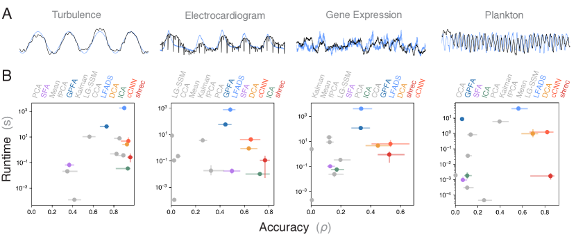
Figure 2: The shared dynamics method discovers causal drivers in diverse datasets. (A) Example driver signals (blue) and their reconstructions (black) from response variables for four different experimental time series. (B) Runtimes versus Spearman correlation scores for different reconstruction methods. Error bars denote bootstrapped one-sided standard errors around random model initializations trained on random subsets of the original time series. The different methods sorted by overall score is overlaid on each plot.

III Results

III.1 The shared dynamics algorithm identifies causal drivers in diverse datasets

In order to demonstrate our method’s practical utility, we perform extensive benchmarks comparing our approach to similar methods. Beyond demonstrating our method’s strong performance as an off-the-shelf method for exploratory data analysis, we aim to highlight how viewing time series through the lens of recurrences potentially represents a physically-motivated method for representing arbitrary sequential datasets.

For our experiments, we apply our method and others to diverse datasets in which a known driving signal influences a large, diverse set of response variables: (1) The turbulent motion of a set of diffusing tracer particles in a double gyre flow. The driver is long-wavelength sinusoidal forcing, while the response variables comprise the radial coordinates of individual particles, as would be observed via Doppler velocimetry. (2) A fetal electrocardiogram time series. The driver is the maternal respiration signal, while the response variables comprise multi-point electrocardiogram recordings placed across the fetal body [55]. (3) Stochastic gene expression dynamics in a subset of the yeast metabolic gene regulatory network, as generated by an experiment design suite used in cell biology [56]. The driver corresponds to the expression level of a known transcriptional regulator in response to a knockdown perturbation, and the response states are the expression levels of downstream genes in the network. (4) Plankton species abundances in an alpine lake in Switzerland over a $20$ year period, as the ecosystem undergoes temperature fluctuations [57]. The driver is the monthly average temperature, and the response variables comprise abundances of individual plankton species interacting through a complex foodweb. $30\%$ of all values in this dataset are missing, presenting a particular challenge to traditional statistical models.

We train unsupervised reconstruction models on only the response time series, and then compare the resulting outputs to the true driving signal. We compare our method to a wide variety of alternative models: principal components analysis (PCA), independent components analysis (ICA), canonical correlation analysis between past and future values (CCA), simple averaging (Mean), a Kalman filter (Kalman), and a surrogate-weighted ensemble Fourier transform (fPCA)[9]. We also consider several recently-introduced dynamical decomposition methods: dynamical components analysis (DCA), which finds low-dimensional modes that maximize predictive information [58]; slow-feature analysis (SFA), which seeks linear combinations of nonlinear kernels that minimize time variation [59]; Gaussian-process factor analysis (GPFA), which finds latent factors parametrizing the mean of a one-step correlated Gaussian process [60]; and a linear Gaussian state space model (LG-SSM) [61]. We also consider artificial neural networks in the form of a causal convolutional network (cCNN), an established architecture for time series representation learning [62]; and Latent Factor Analysis via Dynamical Systems (LFADS), a recurrent variational autoencoder [63]. For all benchmark models we tune hyperparameters using cross-validation and grid search on a separate training dataset than the held-out testing data. We do not vary any hyperparameters for our own method. We use multiple accuracy metrics to compare the reconstructed driver $\hat{z}(t)$ to the true driver $z(t)$, including: mean-squared error, Spearman correlation, covariance, symmetric mean absolute error, mean absolute scaled error, dynamic time warping distance, mutual information, and nonlinear Granger causality; all yield comparable results, and so we report Spearman correlations here for clarity. Additional metrics and benchmark experiments are included in the supplementary material.

We observe consistently strong performance of our approach relative to other methods—both conceptually and computationally simpler methods such as PCA or SFA, but also sophisticated deep-neural-network models like LFADS (Fig. 2). The second strongest-performing benchmark model, the causal autoencoder neural network, takes the hierarchical and sequential structure of time series data into account [62], but otherwise does not specifically exploit potential skew product structure of the underlying time series. Additionally, because our method requires only matrix decomposition and does not require hyperparameter tuning or gradient descent, it is among the fastest methods to compute relative to its performance. We also highlight our method’s strong performance on the plankton ecosystem dataset, which contains fewer overall datapoints and $30\%$ corrupted values, a regime that challenges traditional statistical learning approaches.

Across the experimental datasets, we find that aperiodic driving signals are consistently harder to reconstruct by any method. We speculate that the presence of multiple significant but widely-spaced timescales presents a more challenging problem setting (this motivates our exploration of unstable periodic orbits in the next section). Interestingly, while the turbulent flow contains a monochromatic periodic driver, linear methods like the Fourier transform or PCA are unable to detect this signal due to relatively high noise in the observed data.

We note that many of our example datasets represent cases in which the reconstructed driving signal $\hat{z}(t)$ exerts nearly-instantaneous influence on the response dynamics, $\hat{z}(t)\sim z(t)$. Known as the synchronized regime in prior work [64, 65], we favor this regime for benchmarks both because of the causal identifiability limitation (discussed above), and because the synchronized limit represents the most competitive setting for instantaneous latent variable models like PCA and SFA.

III.2 Chaotic drivers hinder reconstruction, but chaotic responses improve it

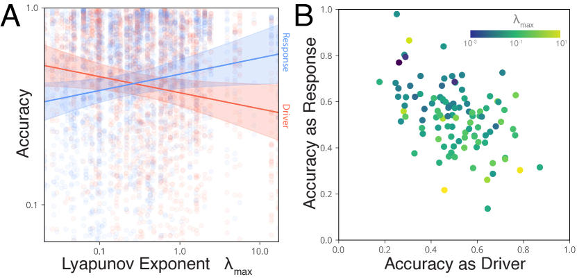
Figure 3: Correlation between chaoticity and accuracy across thousands of dynamical systems. (A) Thousands of random skew-product dynamical systems produced by sampling pairs from a set of $135$ named chaotic systems (e.g. Lorenz, Rössler, etc) and using one system as a driver for replicates of the other system. Linear fits with 95% bootstrapped confidence intervals highlight significant Spearman correlations between the reconstruction accuracy and the Lyapunov exponents of the driver (red, $\rho=0.16\pm 0.03$) and response (blue, $\rho=-0.20\pm 0.03$). (B) For each individual dynamical system, the average accuracy of a reconstruction in which it appears as a response variable, versus one in which it appears as a driver.

In order to further understand which systems are more difficult to reconstruct, we perform an additional benchmark using our recently-introduced database of $135$ low-dimensional ordinary differential equations [66]. Initially curated from published literature to include common systems like the Lorenz, Rössler, and Chua attractors, the dataset has grown through crowdsourcing to span diverse domains such as astrophysics, climatology, and biochemistry. Each system is annotated with estimates of descriptive mathematical properties such as maximum Lyapunov exponents, fractal dimensions, and entropy rates, which quantify different aspects of each system’s underlying complexity.

Using this database, we create random skew-product systems in which one randomly-selected system drives multiple randomly-initialized versions of another randomly-selected system. The Lorenz-Rössler system featured in Figure 1 represents one such skew-product system from the $\sim\!\!\!10^{5}$ possible pairs. We scale the coupling strength to a constant multiple of the average amplitude of both systems, and we scale integration timesteps and trajectory lengths based on precomputed estimates of Lipschitz constants and dominant timescales annotated with each system within our database. We sample all possible system pairs, but retain only time series from the $\leavevmode\nobreak\ 5000$ skew systems that exhibit chaotic dynamics. We apply our reconstruction method to each random skew product time series, and correlate reconstruction accuracy with the separate mathematical properties of the driver and response systems.

We observe weak but consistent negative correlation between the driver Lyapunov exponent and reconstruction accuracy, implying that more chaotic systems are more difficult to reconstruct (Fig. 3A). Surprisingly, we observe the opposite for response systems: more chaotic response systems improve reconstruction quality. As a result, a given dynamical system that proves easier to reconstruct will tend to weaken reconstruction of other systems (Fig. 3B).

This discrepancy arises from the dual roles of the driver and response systems: more chaotic response dynamics produce more diverse and thus informative time series, leading to more unique recurrence events. Conversely, a nearly non-chaotic response system ($\lambda_{max}\approx 0$) yields only a finite amount of information over an extended duration, or across many replicates. Less chaotic systems thus hinder reconstruction because they discover new information about the driver at a slower rate. Conversely, more chaotic drivers transmit information at a faster rate, thus requiring more information to be gained from the response time series. This concept of the driver as an information source, and response systems as receivers, mirrors classical formulations of skew-product systems [67]. The entropy production rate of a chaotic system is bounded from below by the largest Lyapunov exponent [68], which acts as a proxy for the information transmission rate between the driver and response. In the limit of a perfectly lossless transmission from driver to response system, the systems would exhibit generalized synchronization, in which the response becomes a function of solely the driver state [53].

III.3 Accurate reconstruction requires a percolation transition in the time series adjacency graph.

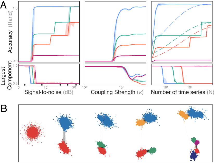
Figure 4: A period-doubling bifurcation reveals that percolation loss precedes accurate reconstruction. (A) Driver reconstruction accuracy (adjusted Rand index) for responses driven by the logistic map in its period-2 (blue), period-4 (turquoise), period-8 (red), and fully-chaotic (magenta) regimes; plotted from left to right as a function of the noise level, driver to response coupling strength, and number of response time series. In the last plot, dashed guides indicate null hypotheses for scaling of accuracy with dataset size, as predicted by the $\beta$-distribution. (Lower) The size of the largest connected component (a measure of percolation) in the reconstructed time series adjacency graph. All plots show median and interquartile range across $60$ replicates with random initial conditions and algorithm seeds. (B) Changes in inferred adjacency graph of the period-8 sequence as the data noise is varied; frames correspond to points on the red trace marked with dots in the first panel.

Our reconstruction method implicitly defines a diffusion process on the time series adjacency graph. In order to understand how this dynamical process couples to the dynamics of the driver itself, we apply our algorithm to response systems driven by the logistic map as it undergoes a series of period-doubling bifurcations leading to chaos (Fig. 4A). We track the point-wise accuracy of the reconstructed discrete driver using the adjusted Rand index, which accounts for the permutation invariance of labels: an adjusted Rand index of $0$ implies a driver state labelling with no greater accuracy than random chance, while a score of one implies that every driver state is correctly identified for each of the $3\times 10^{3}$ timepoints tested. We evaluate our method’s properties by recording its accuracy as a function of three control parameters: the relative amount of stochasticity present in the response dynamics (signal-to-noise ratio), the strength of coupling between the response dynamics and driver, and the number of response time series used for reconstruction $N$. In the latter case, we naively expect that reconstruction accuracy will increase proportionally to the total number of recurrences observed and thus $N$, resulting in an accuracy scaling given by the $\beta$-distribution, which describes the distribution of the expected value of the mean of a binomial process, if driver recurrence states are discovered at random.

We observe that shorter-period drivers are generally easier to reconstruct. Interestingly, at higher-period driving rates, we observe a staircase pattern in the accuracy as reconstruction quality improves. This occurs because, at lower accuracies and longer periods, our approach fails to differentiate all driver states, resulting in groups of states merging together into a coarse-grained, lower-period driving signal. These clusters split into distinct driver substates as reconstruction quality improves (Fig. 4B).

In order to understand how changes in method accuracy depend on structural properties of the underlying recurrence graph, for each condition we measure the order parameter $T_{LCC}/T\in[0,1]$, where $T$ is the total number of nodes and $T_{LCC}$ is the number of nodes comprising the largest connected component. This order parameter detects percolation in finite-size undirected networks [69], and in our system it reveals a first-order phase transition preceding an increase in accuracy when any of the three control parameters is varied. Intuitively, a highly-connected time series network contains many equivalent paths between two nodes, producing ambiguity regarding the correct assignment of recurrence events to driver states. This degeneracy below the percolation transition produces an underdetermined reconstruction, which becomes determined as the amount or quality of response datasets increases. Considering a diffusion process on the recurrence graph, increasing any of the three control parameters increases the duration of transients that reveal almost-invariant structure. The percolation transition therefore indicates the onset of weak ergodicity breaking, in which the dynamics transition from having a short mixing time to a much longer time dominated by gradual leakage between highly-connected groups of nodes sharing the same driver state.

Our observations mirror recent results reporting equivalency between the fitting accuracy of deep artificial neural networks and the jamming transition [70]. By decreasing the ratio of data to model size, a deep neural network passes from underfitting to overfitting regimes mirroring a dilute-to-jammed transition. In our system, increasing training data size or effective size (by decreasing noise or increasing coupling) increases final accuracy by making the time series adjacency graph more dilute—thereby ensuring that well-defined distinctions emerge among different driver states. Our observation that high-period driver states initially appear as low-period states at the onset of the percolation transition is reminiscent of transformations of dynamical systems under the action of a renormalization operator [71].

III.4 Reconstruction shadows dominant unstable periodic orbits.

We next consider the process by which our method learns to reconstruct diverse signals. We return to our original demonstration, in which the Rössler dynamical equations drive many randomly-corrupted measurements of the Lorenz system. We repeat the reconstruction while varying the number of response series $N$, and thus the reconstruction accuracy (Fig. 5).

Given our method’s emphasis on inferring driver recurrence states, we speculate that its accuracy implicitly depends on the unstable periodic orbit spectrum of the driver [22]. Classical work on nonlinear dynamical systems has shown that any chaotic system can be decomposed into an infinite set of unstable periodic orbits [72], which trajectories shadow for extended durations proportional to each orbit’s relative stability. While chaotic systems have continuous power spectra, the set of valid unstable periodic orbits bears basic topological restrictions due to attractor geometry—making it a countable, albeit infinite, hierarchical measure for the dynamical system. We compute several unstable periodic orbits of the Rössler driving system using the method of closest recurrences [73], and select the three most dominant orbits based on the relative duration they are shadowed by the driver dynamics.

Comparing the pairwise distance matrix of the reconstructed signal with the distance matrix of individual unstable periodic orbits suggests that, as the amount of training data increases, the reconstructed distance matrix initially approximates only the most dominant orbit, but then gradually approximates finer-scale details of the driver attractor that are encoded in secondary orbits. We hypothesize that the recurrence structure of our method biases it towards shorter-period and more stable orbits that dominate the graph partition. This phenomenon provides some context for our earlier observation that reconstruction accuracy depends inversely on the driver’s Lyapunov exponent: systems with larger Lyapunov exponents tend to transition among a larger set of orbits, thus requiring more recurrence information to produce faithful reconstructions [74].

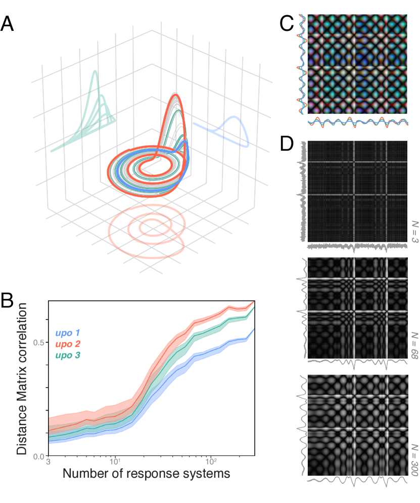
Figure 5: Reconstruction of complex signals follows dominant unstable periodic orbits. (A) The three most stable unstable periodic orbits for the Rössler system. (B) Elementwise Pearson correlation between the distance matrix of the reconstructed Rössler driver and the three orbits, as the number of response time series (and thus overall driver reconstruction accuracy) increases. Ranges denote 95% confidence intervals around random model initializations trained on random subsets of available response series. (C) The overlaid true distance matrices of the three leading orbits, with RGB channels of the color image encoding each orbit’s individual distance matrix. (D) The distance matrices of the reconstruction as the number of response subsystems increases.

IV Discussion

We have presented a theoretically-motivated unsupervised learning method that reconstructs an unobserved causal driving signal, given observations of downstream response variables. Across extensive benchmarks against methods drawn from diverse domains, we find that our method quickly and robustly reconstructs diverse driving signals in time series datasets ranging from fluid dynamics to systems biology. Beyond introducing a new general-purpose data analysis method, our work provides empirical insight into the nature of information transmission in coupled dissipative systems: the topology of the driver’s characteristic unstable orbits manifests as structure within the recurrence graph of the response time series, with the efficiency of this linkage mediated by both the chaoticity of the driver, and the diversity of the responses. A diffusion process on the resulting time series graph reveals driver structure in its longest-lived transient modes, and methods that increase the lifetime of these transients—such as more response datasets, increased driver-response coupling, or reduced measurement noise—produce a corresponding increase in reconstruction accuracy. Diffusion represents a heuristic solution to the difficult combinatorial optimization problem of graph traversal and topological node sorting, and our method reduces to a previously-known exact algorithm in the limit of a noiseless and discrete periodic driver [23].

Key limitations of our approach therefore stem from our use of diffusive dynamics for graph traversal. Certain measurement types may induce false recurrence events with systematic structure, such as sensor saturation or memory effects, that impose fixed structural barriers to diffusion on the graph adjacency matrix—akin to inhomogenous diffusivity. Mitigating such effects requires sufficient information about the measurement dynamics to reconstruct and correct for response bias; within our framework, this might require preconditioning the graph Laplacian [75]. Additionally, non-stationary driving signals can complicate reconstruction; for example if the attractor is time-dependent (e.g. energy gradually dissipates due to drag), then the driver may exhibit transient chaos before settling into a state of quiescence or oscillation [76]. In this case, a random walker’s transitions among nodes will no longer heed detailed balance and the transition operator will exhibit non-Hermitian structure, resulting in long-lived nonequilibrium steady-states that complicate driver state assignment [77, 78, 79]. These and other, more challenging data types may require nonlinear alternatives to diffusion processes on the recurrence graph. Our use of diffusion therefore represents a form of inductive bias in the time series representations learned by our model.

However, the problem of discovering nonlinear processes from an empirical recurrence graph introduces a variety of potential generalizations grounded in recent results from statistical learning. Instead of directly fitting a linear operator, future work could leverage recent methods for data-driven inference of dynamical propagators [80, 81, 82, 83], which can even produce reduced-order analytical models [84]. Generalizations may also incorporate new graph representation or traversal methods (such as message passing)[51, 85], particularly graph neural networks [86, 87]. Thus, beyond our specific algorithm, our work motivates general parametrization of time series models in terms of recurrences, and the latent orbit structure that they encode.

V Acknowledgments

We thank Phil Morrison, Harry Swinney, and Michael Marder for discussions. We thank Anthony Bao for feedback on the manuscript. W. G. was supported by the University of Texas at Austin. Computational resources for this study were provided by the Texas Advanced Computing Center (TACC) at The University of Texas at Austin.

VI Code availability

All code used in this study is available online at https://github.com/williamgilpin/shrec

References

- [1] Rosenblatt, A. E. & Schmitz, O. J. Climate change, nutrition, and bottom-up and top-down food web processes. Trends in Ecology & Evolution 31, 965–975 (2016).
- [2] Cande, J. et al. Optogenetic dissection of descending behavioral control in drosophila. Elife 7 (2018).
- [3] Leisner, M., Stingl, K., Frey, E. & Maier, B. Stochastic switching to competence. Current opinion in microbiology 11, 553–559 (2008).
- [4] Pezzulo, G. & Levin, M. Top-down models in biology: explanation and control of complex living systems above the molecular level. Journal of The Royal Society Interface 13, 20160555 (2016).
- [5] Schwarze, A. C., Ichinaga, S. M. & Brunton, B. W. Network inference via process motifs for lagged correlation in linear stochastic processes. arXiv preprint arXiv:2208.08871 (2022).
- [6] Runge, J., Heitzig, J., Petoukhov, V. & Kurths, J. Escaping the curse of dimensionality in estimating multivariate transfer entropy. Physical review letters 108, 258701 (2012).
- [7] Sugihara, G. et al. Detecting causality in complex ecosystems. science 338, 496–500 (2012).
- [8] Runge, J., Nowack, P., Kretschmer, M., Flaxman, S. & Sejdinovic, D. Detecting and quantifying causal associations in large nonlinear time series datasets. Science Advances 5, eaau4996 (2019).
- [9] Kantz, H. & Schreiber, T. Nonlinear time series analysis, vol. 7 (Cambridge University Press, 2004).
- [10] Munch, S. B., Rogers, T. L. & Sugihara, G. Recent developments in empirical dynamic modelling. Methods in Ecology and Evolution (2022).
- [11] Runge, J. et al. Inferring causation from time series in earth system sciences. Nature communications 10, 1–13 (2019).
- [12] De Brouwer, E., Arany, A., Simm, J. & Moreau, Y. Latent convergent cross mapping. In International Conference on Learning Representations (2020).
- [13] Bennett, S. & Yu, R. Rethinking neural relational inference for granger causal discovery. In NeurIPS 2022 Workshop on Causality for Real-world Impact (2022).
- [14] Quiroga, R. Q., Arnhold, J. & Grassberger, P. Learning driver-response relationships from synchronization patterns. Physical Review E 61, 5142 (2000).
- [15] Takens, F. Detecting strange attractors in turbulence. In Dynamical systems and turbulence, Warwick 1980, 366–381 (Springer, 1981).
- [16] Packard, N. H., Crutchfield, J. P., Farmer, J. D. & Shaw, R. S. Geometry from a time series. Physical Review Letters 45, 712 (1980).
- [17] Stark, J. Delay embeddings for forced systems. i. deterministic forcing. Journal of Nonlinear Science 9, 255–332 (1999).
- [18] Sober, S. J., Sponberg, S., Nemenman, I. & Ting, L. H. Millisecond spike timing codes for motor control. Trends in neurosciences 41, 644–648 (2018).
- [19] Dhamala, M., Rangarajan, G. & Ding, M. Estimating granger causality from fourier and wavelet transforms of time series data. Physical review letters 100, 018701 (2008).
- [20] Mastakouri, A. A., Schölkopf, B. & Janzing, D. Necessary and sufficient conditions for causal feature selection in time series with latent common causes. In International Conference on Machine Learning, 7502–7511 (PMLR, 2021).
- [21] Pecora, L. M., Carroll, T. L., Johnson, G. A., Mar, D. J. & Heagy, J. F. Fundamentals of synchronization in chaotic systems, concepts, and applications. Chaos: An Interdisciplinary Journal of Nonlinear Science 7, 520–543 (1997).
- [22] Hunt, B. R., Ott, E. & Yorke, J. A. Differentiable generalized synchronization of chaos. Physical Review E 55, 4029 (1997).
- [23] Sauer, T. D. Reconstruction of shared nonlinear dynamics in a network. Physical review letters 93, 198701 (2004).
- [24] Wehmeyer, C. & Noé, F. Time-lagged autoencoders: Deep learning of slow collective variables for molecular kinetics. The Journal of chemical physics 148, 241703 (2018).
- [25] Gilpin, W. Deep reconstruction of strange attractors from time series. Advances in Neural Information Processing Systems 33 (2020).
- [26] Bakarji, J., Champion, K., Kutz, J. N. & Brunton, S. L. Discovering governing equations from partial measurements with deep delay autoencoders. arXiv preprint arXiv:2201.05136 (2022).
- [27] Mezard, M. & Montanari, A. Information, physics, and computation (Oxford University Press, 2009).
- [28] Froyland, G. & Padberg, K. Almost-invariant sets and invariant manifolds—connecting probabilistic and geometric descriptions of coherent structures in flows. Physica D: Nonlinear Phenomena 238, 1507–1523 (2009).
- [29] Brunton, S. L., Brunton, B. W., Proctor, J. L., Kaiser, E. & Kutz, J. N. Chaos as an intermittently forced linear system. Nature communications 8, 1–9 (2017).
- [30] Mezić, I. Spectral properties of dynamical systems, model reduction and decompositions. Nonlinear Dynamics 41, 309–325 (2005).
- [31] Costa, A. C., Ahamed, T., Jordan, D. & Stephens, G. Maximally predictive ensemble dynamics from data. arXiv preprint arXiv:2105.12811 (2021).
- [32] Giannakis, D. & Majda, A. J. Nonlinear laplacian spectral analysis for time series with intermittency and low-frequency variability. Proceedings of the National Academy of Sciences 109, 2222–2227 (2012).
- [33] Girvan, M. & Newman, M. E. Community structure in social and biological networks. Proceedings of the national academy of sciences 99, 7821–7826 (2002).
- [34] Rogers, T. L. & Munch, S. B. Hidden similarities in the dynamics of a weakly synchronous marine metapopulation. Proceedings of the National Academy of Sciences 117, 479–485 (2020).
- [35] Deyle, E. R., Maher, M. C., Hernandez, R. D., Basu, S. & Sugihara, G. Global environmental drivers of influenza. Proceedings of the National Academy of Sciences 113, 13081–13086 (2016).
- [36] Hirata, Y., Horai, S. & Aihara, K. Reproduction of distance matrices and original time series from recurrence plots and their applications. The European Physical Journal Special Topics 164, 13–22 (2008).
- [37] Hirata, Y. & Aihara, K. Identifying hidden common causes from bivariate time series: A method using recurrence plots. Physical Review E 81, 016203 (2010).
- [38] Haghverdi, L., Büttner, M., Wolf, F. A., Buettner, F. & Theis, F. J. Diffusion pseudotime robustly reconstructs lineage branching. Nature methods 13, 845–848 (2016).
- [39] Donner, R. V., Zou, Y., Donges, J. F., Marwan, N. & Kurths, J. Recurrence networks—a novel paradigm for nonlinear time series analysis. New Journal of Physics 12, 033025 (2010).
- [40] Davidsen, J., Grassberger, P. & Paczuski, M. Networks of recurrent events, a theory of records, and an application to finding causal signatures in seismicity. Physical Review E 77, 066104 (2008).
- [41] Myers, A., Munch, E. & Khasawneh, F. A. Persistent homology of complex networks for dynamic state detection. Physical Review E 100, 022314 (2019).
- [42] McCabe, M. & Brown, J. Learning to assimilate in chaotic dynamical systems. Advances in Neural Information Processing Systems 34, 12237–12250 (2021).
- [43] Frerix, T. et al. Variational data assimilation with a learned inverse observation operator. In International Conference on Machine Learning, 3449–3458 (PMLR, 2021).
- [44] Karl, M., Soelch, M., Bayer, J. & Van der Smagt, P. Deep variational bayes filters: Unsupervised learning of state space models from raw data. arXiv preprint arXiv:1605.06432 (2016).
- [45] Krishnan, R. G., Shalit, U. & Sontag, D. Deep kalman filters. arXiv preprint arXiv:1511.05121 (2015).
- [46] Koppe, G., Toutounji, H., Kirsch, P., Lis, S. & Durstewitz, D. Identifying nonlinear dynamical systems via generative recurrent neural networks with applications to fmri. PLoS computational biology 15, e1007263 (2019).
- [47] Hamilton, F., Berry, T. & Sauer, T. Ensemble kalman filtering without a model. Physical Review X 6, 011021 (2016).
- [48] Ye, H. & Sugihara, G. Information leverage in interconnected ecosystems: Overcoming the curse of dimensionality. Science 353, 922–925 (2016).
- [49] Leng, S. et al. Partial cross mapping eliminates indirect causal influences. Nature communications 11, 1–9 (2020).
- [50] Alaa, A. & Van Der Schaar, M. Validating causal inference models via influence functions. In International Conference on Machine Learning, 191–201 (PMLR, 2019).
- [51] Williams, O. E., Lacasa, L., Millán, A. P. & Latora, V. The shape of memory in temporal networks. Nature communications 13, 1–8 (2022).
- [52] Pearl, J. Causal inference. Causality: objectives and assessment 39–58 (2010).
- [53] Pecora, L. M. & Carroll, T. L. Synchronization in chaotic systems. Physical Review Letters 64, 821 (1990).
- [54] Hegger, R., Kantz, H., Matassini, L. & Schreiber, T. Coping with nonstationarity by overembedding. Physical Review Letters 84, 4092 (2000).
- [55] Sulas, E. et al. A non-invasive multimodal foetal ecg–doppler dataset for antenatal cardiology research. Scientific Data 8, 1–19 (2021).
- [56] Schaffter, T., Marbach, D. & Floreano, D. Genenetweaver: in silico benchmark generation and performance profiling of network inference methods. Bioinformatics 27, 2263–2270 (2011).
- [57] Pomati, F., Shurin, J. B., Andersen, K. H., Tellenbach, C. & Barton, A. D. Interacting temperature, nutrients and zooplankton grazing control phytoplankton size-abundance relationships in eight swiss lakes. Frontiers in Microbiology 10, 3155 (2020).
- [58] Clark, D., Livezey, J. & Bouchard, K. Unsupervised discovery of temporal structure in noisy data with dynamical components analysis. Advances in Neural Information Processing Systems 32 (2019).
- [59] Wiskott, L. & Sejnowski, T. J. Slow feature analysis: Unsupervised learning of invariances. Neural computation 14, 715–770 (2002).
- [60] Yu, B. M. et al. Gaussian-process factor analysis for low-dimensional single-trial analysis of neural population activity. Advances in neural information processing systems 21 (2008).
- [61] Särkkä, S. Bayesian filtering and smoothing. 3 (Cambridge university press, 2013).
- [62] Franceschi, J.-Y., Dieuleveut, A. & Jaggi, M. Unsupervised scalable representation learning for multivariate time series. Advances in neural information processing systems 32 (2019).
- [63] Pandarinath, C. et al. Inferring single-trial neural population dynamics using sequential auto-encoders. Nature methods 15, 805–815 (2018).
- [64] Mønster, D., Fusaroli, R., Tylén, K., Roepstorff, A. & Sherson, J. F. Causal inference from noisy time-series data—testing the convergent cross-mapping algorithm in the presence of noise and external influence. Future Generation Computer Systems 73, 52–62 (2017).
- [65] Ye, H., Deyle, E. R., Gilarranz, L. J. & Sugihara, G. Distinguishing time-delayed causal interactions using convergent cross mapping. Scientific reports 5, 1–9 (2015).
- [66] Gilpin, W. Chaos as an interpretable benchmark for forecasting and data-driven modelling. Advances in Neural Information Processing Systems 1 (2021).
- [67] Adler, R., Coppersmith, D. & Hassner, M. Algorithms for sliding block codes-an application of symbolic dynamics to information theory. IEEE Transactions on Information Theory 29, 5–22 (1983).
- [68] Pesin, Y. Characteristic lyapunov exponents and smooth ergodic theory. Russian Mathematical Surveys 32, 55 (1977).
- [69] Hébert-Dufresne, L. & Allard, A. Smeared phase transitions in percolation on real complex networks. Physical Review Research 1, 013009 (2019).
- [70] Geiger, M. et al. Jamming transition as a paradigm to understand the loss landscape of deep neural networks. Physical Review E 100, 012115 (2019).
- [71] Feigenbaum, M. J. The universal metric properties of nonlinear transformations. Journal of Statistical Physics 21, 669–706 (1979).
- [72] Cvitanović, P. Invariant measurement of strange sets in terms of cycles. Physical Review Letters 61, 2729 (1988).
- [73] Lathrop, D. P. & Kostelich, E. J. Characterization of an experimental strange attractor by periodic orbits. Physical Review A 40, 4028 (1989).
- [74] Ott, E. Chaos in dynamical systems (Cambridge University Press, 2002).
- [75] Krishnan, D., Fattal, R. & Szeliski, R. Efficient preconditioning of laplacian matrices for computer graphics. ACM transactions on Graphics (tOG) 32, 1–15 (2013).
- [76] Motter, A. E., Gruiz, M., Károlyi, G. & Tél, T. Doubly transient chaos: Generic form of chaos in autonomous dissipative systems. Physical review letters 111, 194101 (2013).
- [77] Fruchart, M., Hanai, R., Littlewood, P. B. & Vitelli, V. Non-reciprocal phase transitions. Nature 592, 363–369 (2021).
- [78] Battle, C. et al. Broken detailed balance at mesoscopic scales in active biological systems. Science 352, 604–607 (2016).
- [79] Weis, C. et al. Coalescence of attractors: exceptional points in non-linear dynamical systems. arXiv preprint arXiv:2207.11667 (2022).
- [80] Bramburger, J. J., Kutz, J. N. & Brunton, S. L. Data-driven stabilization of periodic orbits. IEEE Access 9, 43504–43521 (2021).
- [81] Raissi, M. & Karniadakis, G. E. Hidden physics models: Machine learning of nonlinear partial differential equations. Journal of Computational Physics 357, 125–141 (2018).
- [82] Chen, R. T., Rubanova, Y., Bettencourt, J. & Duvenaud, D. K. Neural ordinary differential equations. Advances in neural information processing systems 31 (2018).
- [83] Choudhary, A. et al. Physics-enhanced neural networks learn order and chaos. Physical Review E 101, 062207 (2020).
- [84] Champion, K., Lusch, B., Kutz, J. N. & Brunton, S. L. Data-driven discovery of coordinates and governing equations. Proceedings of the National Academy of Sciences 116, 22445–22451 (2019).
- [85] Gilmer, J., Schoenholz, S. S., Riley, P. F., Vinyals, O. & Dahl, G. E. Neural message passing for quantum chemistry. In International conference on machine learning, 1263–1272 (PMLR, 2017).
- [86] Donoho, D. L., Maleki, A. & Montanari, A. Message-passing algorithms for compressed sensing. Proceedings of the National Academy of Sciences 106, 18914–18919 (2009).
- [87] Rossi, E. et al. Temporal graph networks for deep learning on dynamic graphs. arXiv preprint arXiv:2006.10637 (2020).