Calculating Point Spread Functions: Methods, Pitfalls and Solutions

Abstract

We discuss advantages and disadvantages of various ways of calculating an optical Point Spread Function (PSF) and present novel Fourier-based techniques for computing vector PSF. The knowledge of the exact structure of the PSF of a given optical system is of interest in fluorescence microscopy to be able to perform high-quality image reconstructions. Even, if we know how an aberrant optical path deviates from the original design, the corresponding PSF is often hard to calculate, as the phase and amplitude modifications need to be modelled in detail. Accurate PSF models need to account for the vector nature of the electric fields in particular for high numerical apertures. Compared to the computation of a commonly used scalar PSF model, the vectorial model is computationally more expensive, yet more accurate. State-of-the-art scalar and vector PSF models exist, but they all have their pros and cons. Many real-space-based models fall into the sampling pitfall near the centre of the image, yielding integrated plane intensities which are not constant near the nominal focus position, violating energy conservation. This and other problems which typically arise when calculating PSFs are discussed and their shortfalls are quantitatively compared. A highly oversampled Richards and Wolf model is chosen as the gold standard for our quantitative comparison due its ability to represent the ideal field accurately, albeit being practically very slow in the calculation. Fourier-based methods are shown to be computationally very efficient and radial symmetry assumption are not needed making it easy to include non-centro-symmetric aberrations. For this reason newly presented methods such as the SincR and the Fourier-Shell method are essentially based on multidimensional Fourier-transformations.

Keywords: point spread function, Fourier optics, fluorescence microscopy

I Introduction

Aplanatic imaging systems strive to image a plane in the object to the detector plane (e.g. a CCD camera) Singer, Totzeck, and Gross (2005). To achieve this, any optical system needs to fulfill the Abbe sine condition Gu (2000). This condition relates any angle of a beam emitted by the sample ($\theta_{\text{em}}$) to its corresponding angle reaching the detector ($\theta_{\text{det}}$), and is given by $\sin(\theta_{\text{em}})/\sin(\theta_{\text{det}})=M$, with $M$ being the magnification of the optical system in terms of geometric optics Gu (2000); Singer, Totzeck, and Gross (2005). As shown in the thin lens approximation in Fig. 1, a simple $4f$-imaging microscope imaging system with a magnification of $M=2$ would not fulfill the above-mentioned Abbe sine condition.

Figure 1: Geometrical representation of a $4$f-imaging system using the thin lens approximation. Note that here $\tan(\theta_{\text{em}})/\tan(\theta_{\text{det}})=f_{2}/f_{1}$, which violates Abbe's sine condition. BFP stands for back focal plane. Here lens 1 corresponds to the microscope objective lens while lens 2 represents the tube lens.

The simplicity of such drawings can be maintained by introducing the concept of the Gaussian reference sphere (see Fig. 2) describing the equivalent refractive loci for aplanatic imaging systems. A Gaussian reference sphere is a sphere centred where the object plane (the plane to image) or at the focus position (in image plane) intersect the optical axis. Its radius is equal to the focal length $f_{1}$ or $f_{2}$ in each of the corresponding planes (Singer, Totzeck, and Gross, 2005). The rays propagate to the Gaussian reference sphere and get teleported without acquiring any extra phase to a reference plane, which is a plane surface parallel to the pupil plane in the back focal plane (BFP), indicated by the positions of the planes of lens 1 and lens 2 in Fig. 1. The same principle is applied in reverse to the tube lens (lens 2 in Fig. 1), where the effect can often be neglected due to the usually large magnification of the objective and thus small angles (see right side of Fig. 2).

Figure 2: Introduction refraction at the Gaussian reference sphere warrants that $\sin(\theta_{\text{em}})/\sin(\theta_{\text{det}})=f_{2}/f_{1}$ is a constant and the system therefore satisfies Abbe's sine condition. "Teleportation" means that the beams are continued at the connected surface without acquiring any phase for the space in between the plane reference plane and Gaussian reference sphere.

If this task of imaging a plane to a plane is performed well by a careful design, the structure of an image of point object, called the point spread function (PSF) does, to a very good approximation, not change with location over the field of view of the optical system. The image of an incoherently emitting sample can well be described by a convolution of the object emitter density with the PSF. Such imaging systems are typically called linear shift invariant imaging systems (Goodman, 2005).

Here we discuss calculating PSFs using various computational tools. An accurate PSF model is an important requirement for a successful image reconstruction Sage et al. (2017). Various studies have been conducted to model the PSF of a given optical system Haeberlé (2003); Gibson and Lanni (1989); Richards and Wolf (1959); Li, XUE, and BLU (2017); Aguet et al. (2009); Kirshner et al. (2013). The computation of each of these models has pros and cons, some of which we will discuss below. In Section II, we firstly introduce the readers to the state-of-the-art scalar and vector PSF models. Secondly, we present ingredients for computing our novel methods using Fourier optics III. The fast Fourier-transformation is a very handy tool to speed up PSF calculations, but its pitfalls need to be carefully avoided. We therefore present the pitfalls that one may encounter in the calculation and ways around them. In Section IV, we describe in detail novel Fourier-based techniques for computing vector PSFs. Finally, in Section V the various methods are compared quantitatively in terms of their accuracy and computation time. A further aim of this manuscript is to release a toolbox to the scientific community, which others can benefit from for calculating PSFs using uniform or modified (aberrated) apertures Holinirina Dina Miora, Kielhorn, and Heintzmann (2022).

II Existing PSFs models

A scalar PSF model is computed from one integral per point, $(x,y,z)$. It is considerably cheap computationally. However, it does account for the vector nature of the electric field describing the light which will lead to a wrong estimation of the field at higher aperture angles. A vector PSF, on the other hand, requires a calculation of all the three spatial components of the electric field (Gibson and Lanni, 1989). It is more accurate as it carries more information about the field such its polarization state (Wolf, 1959). The Richards and Wolf (RW) vector PSF model has been shown to represent a vector field to a very high accuracy (Richards and Wolf, 1959; Török and Varga, 1997; Kirshner et al., 2013). Yet, the implementation of the RW model still has its limitations in terms of sampling and computation time as we will discuss below.

II.1 Scalar PSF model

A well-known scalar PSF model was developed by Gibson and Lanni (GL) (Gibson and Lanni, 1989). The model is valid within the Kirchhoff boundary conditions for scalar diffraction theory (Gibson and Lanni, 1989). The expression of the PSF as per the GL model at a position $(x,y,z)$ is given by:

$$\text{PSF}(x,y,z;\textbf{p})=\\ \left|\text{A}\int_{0}^{1}\exp\left(ik\Phi(\rho,z,\textbf{p})\right)J_{0}(kr\text{NA}\rho)\rho d\rho\right|^{2},$$ (1)

where $r=\sqrt{x^{2}+y^{2}}$, $A$ is a constant complex amplitude, $\rho$ is the normalized radius in the back focal plane, $\Phi$ is aberration function and, p is a vector summarizing optical characteristic such as refractive indices and thicknesses of of aberrant surfaces in the system. In our calculation, we consider a case where the actual condition is assumed to meet the design condition of the imaging system (Gibson and Lanni, 1991).

II.2 The Richards and Wolf Model (RW)

II.2.1 Description of the model

A scalar electric field model is limited to only a single complex amplitude over the image space. It does not give any information about the polarization state of the image field, the direction of the energy flow and it is also not applicable to imaging at high numerical apertures (Wolf, 1959). Richards and Wolf described the focusing of electromagnetic waves for low and high numerical aperture using an angular spectrum of plane waves in an integral representation (Richards and Wolf, 1959). The model is a vector formulation of the scalar Debye model. The expressions of the electric field from a point source $S_{0}$ at time $t$ at a position $(x,y,z)$ in the image space is as follows:

$$\vec{E}(x,y,z,t)=\mathcal{R}\{\vec{\mathcal{A}}_{E}(x,y,z)\exp(i\varpi t)\}$$ (2)

where $\vec{\mathcal{A}}_{E}$ is the amplitude vector, $\varpi$ the angular frequency of the point source and $\mathcal{R}\{\}$ denotes taking the real part. The amplitude vector satisfies the independent wave equation and is given by:

$$\vec{\mathcal{A}}_{E}(x,y,z)=\begin{cases}-ia\left(I_{0}+I_{2}\cos 2\phi_{xy}\right)\\ -iaI_{2}\sin 2\phi_{xy}\\ -2aI_{1}\cos 2\phi_{xy}\end{cases}$$ (3)

with the constant $a$ and

$$\begin{cases}I_{0}=\int_{0}^{\alpha}\cos^{1/2}\theta\sin\theta(1+\cos\theta)J_{0}(kr\sin\theta)e^{ikz\cos\theta}d\theta\\ I_{1}=\int_{0}^{\alpha}\cos^{1/2}\theta\sin^{2}\theta J_{1}(kr\sin\theta)e^{ikz\cos\theta}d\theta\\ I_{2}=\int_{0}^{\alpha}\cos^{1/2}\theta\sin\theta(1-\cos\theta)J_{2}(kr\sin\theta)e^{ikz\cos\theta}d\theta\end{cases}$$ (4)

$\alpha$ is the maximum angular aperture, $J_{j}$ is the Bessel function of order $j$, the integration variable $\theta$ correspond to the angle a point on the Gaussian reference sphere has to the optical axis, $r=\sqrt{x^{2}+y^{2}}$ as well as $\phi_{xy}$ relate to the point where the field is evaluated, with $\phi_{xy}$ being the azimuth at $(x,y,z)$ (Richards and Wolf, 1959). The term $\cos^{1/2}\theta$ in Eq. 4 is the aplanatic factor for energy conservation, illuminating the objective with a plane wave. These equations rely on the Kirchhoff boundary conditions and only consider homogeneous waves (Wolf, 1959). An inhomogeneous wave corresponds to a field which decays for a large propagation distance whereas the Kirchhoff boundary conditions imply that only incident field within the opening aperture of the exit pupil contribute to the field at $(x,y,z)$ in the image space.

II.2.2 Computation

There exist different ways for computing the three integrals in Eq. (4). One way could consist of evaluating the integration numerically. To improve the accuracy, finer steps of integration are needed which can lead to an expensive computation. One technique that we denote by RW₁ exploits a cylindrical coordinate system to perform the integration. This has computational advantages, since only a two-dimensional $rz$-map (i.e. a centered radial axis versus axial $z$) has to be calculated for $I_{0},I_{1}$ and $I_{2}$, since their definition is independent of the azimuth. However, this procedure may have the disadvantage that we cannot easily include arbitrary aperture modifications which do not possess circular symmetry into the model. If there is no need for calculating the electric field but only the intensity, this technique has a shorter path to compute the intensity. We denote this shorter path by RW₀.

The second method that has been developed in this work, denoted by RW₂, uses a Fourier transform along the optical $z$ axis (see Section IV.2.3) to compute the $(x,y,z)$ components $I_{0},I_{1}$ and $I_{2}$ in Eq. (4). We choose as a variable of integration $\xi=\cos\theta$. RW₂ is on average $1.45$ times slower than RW₁. However, it does not require in its computation the radial symmetry property of a PSF while RW₀ and RW₁ do.

II.3 State-of-the-art PSFs models

Four state-of-the-art commonly used PSF models were chosen to compare our methods to. The first model is a scalar PSF based on the work of Gibson and Lanni (1989), and further developed by Li, XUE, and BLU (2017). This technique calculates the PSF fast by using a combination of Bessel series. The second and third models are a scalar and vector PSF as described in Aguet et al. (2009). The PSFs are computed using a numerical integration based on Simpson’s rule. The last state-of-the-art PSF that we compare with is a vector PSF calculated with the Richards and Wolf $3$D optical model from the PSFGenerator toolbox in (Kirshner et al., 2013). Each of those models have their advantages, as well as their limitations as we discuss in Section V.

III Tools for computing a vector PSF using Fourier optics

III.1 Scalar high numerical aperture (NA) model

To start with the PSF calculation using a Fourier optic formulation, let us first consider the calculation of the intensity distribution near the nominal focus when focusing a monochromatic coherent plane wave by a high-NA microscopy objective (Fig. 3). The beam is entering the objective system from the left side and is spatially limited by the entrance pupil of the optical system, corresponding to the image of the aperture stop as created by the optics to the right of the aperture (see Fig. 3). An “aperture stop”, is in practice either intentionally introduced to warrant the linear shift invariant performance of the system and to avoid aberrations from unwanted beams, or effectively provided by the inner geometry of the objective. The limitation of the beams is therefore approximated to be at the limit of that aperture stop. At this pupil plane, every point $P_{W}$ on the wavefront is considered as a source of a Huygens wavelet, denoted by $W$ (Crew, 2009).

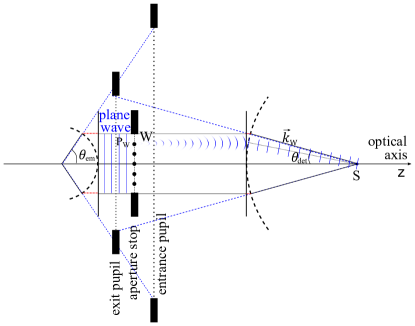
Figure 3: Visualization of the pupils and representation of the Huygens Wavelet becoming a plane wave.

Firstly, we limit ourselves to a scalar electric field, where the field is a directionless value and only a function of its position in space. The vector nature of the electric field will be introduced further down below. The aperture plane can be seen as a superposition of spherical wavelets, each of which gives rise to a plane wave after the objective directed towards the nominal focus point S (see the wavelet labelled “W” in Fig. 3). According to the Huygens-Fresnel principle, the spherically converging wave is obtained by superimposing all these wavelets (Crew, 2009). The superimposed wavelets have to acquire exactly the same optical path length and constructively interfere at S. In other words, the phase at the nominal focus is identical for all such wavelets and can thus be set to zero in our simulation. For convenience, we choose S as the center of our real-space coordinate system. The wavelet W giving rise to a plane wave in focus (Fig. 3) can now conveniently be described in Fourier space as a single point P${}_{\text{W}}$ (Fig. 4), i.e. a single $3$-dimensional vector ($\vec{k}_{W}$) in Fourier space. Such vectors have all to necessarily reside on a sphere of a radius $k_{0}=2\pi/\lambda_{\text{em}},\lambda_{\text{em}}=\lambda/n,$ $\lambda_{\text{em}}$ and $\lambda$ being the emission and the corresponding vacuum wavelengths respectively, and $n$ the refractive index of the embedding medium.

(a)

(b)

Figure 4: (a) Coordinate system in Fourier space: $\theta$ and $\phi$ are the elevation and azimuthal angles respectively. (b) Fourier space representation of a plane wave from a wavelet W at a point source P${}_{\text{W}}$ in the pupil plane called McCutchen pupil (bold black line). The $k_{y}-$axis in (b) is oriented towards the front plane of the paper.

A pupil position in real space corresponds to the lateral component $\vec{k}_{x}$ of the wave-vector $\vec{k}$. This linear correspondence is forced by the Abbe sine condition between the pupil plane coordinate and the $k$-vector position of the wave near the focal plane.

The pupil plane aperture stop thus gives rise to a three-dimensional cap residing on the $k$-sphere in Fourier space (see solid cap in Fig. 4b in the Fourier space representation). As the aperture is limited by the NA of the objective, the $3$D frequency spectrum in Fourier space is represented in a segment of the $k$-sphere sphere. This segment is called “generalized aperture” or “McCutchen pupil” (McCutchen, 1964).

To now calculate the (complex-valued) amplitude distribution in real space near the focus S, we need to generate a three-dimensional McCutchen pupil of uniform amplitude and perform an inverse three-dimensional Fourier transformation. The Fourier-based PSF models that are presented in this work are based on this understanding. The four different methods differ in how the amplitude on the McCutchen pupil is caculcated and how the field is propagated in the homogeneous medium. To the best of our knowledge, these approaches have not been previously described elsewhere. Each method has its own advantages, pitfalls and drawbacks as discussed in the next section.

It is instructive to first limit ourselves to the calculation of the $xy$-plane at the nominal focus position $z=0$. We can interpret this plane as being a slice of the three-dimensional focus volume, i.e. a multiplication with $\delta(z=0)$. In Fourier space such a $z$-slice in real space corresponds to an integral of the amplitude over $k_{z}$ according to the Fourier-slice theorem (Goodman, 2005). Since the McCutchen pupil is infinitely thin, and only waves along the positive $z$ direction, i.e. positive $k_{z}$, contribute to the focus, there is a bijective mapping from the 3D McCutchen pupil to its 2D projection. This establishes a direct correspondence between the pupil plane amplitude and the two-dimensional Fourier transformation of the $xy$-amplitude at the focus.

Slicing at a different $z$-position, $z_{1}$, can be seen as a translation by $z_{1}$ along $z$ which amounts to a phase-change by $\exp\left(iz_{1}k_{z}\right)$ which can be written as $\exp\left(iz_{1}\sqrt{k_{0}^{2}-k_{r}^{2}}\right)$. In this projection over $k_{z}$ we may need to account for the effect of the local orientation of the McCutchen pupil via a projection factor and for possible other factors as given below in a more detailed analysis regarding the Gaussian reference sphere.

III.2 Vector electric field

The above discussion assumed a scalar field (e.g. as common in acoustics). However, the electric field is described by a spatially varying amplitude field vector with three complex components $\vec{E}=(E_{x},E_{y},E_{z})$ of the form $E_{x,y,z}(r)=\mathcal{A}_{x,y,z}(r)\exp(i\varpi t)$ where the amplitude, $\mathcal{A}_{x,y,z}(r)$, is a function of the position $r$ where the field is evaluated and $\exp(i\varpi t)$ is the time dependent phasor, $\varpi$ being the angular frequency and $t$ the time. Since we stay in the realm of linear optics, where the interaction between the excitation light and matter is achieved linearly, we continue our considerations with the assumption that the PSF (i.e. the excitation of a weakly excited fluorophore) is given by a linear dependence to the local irradiance: $I=|\vec{E}|^{2}$. All of the Fourier-space considerations as stated for the scalar field above can now be applied individually to each of the components of the amplitude field vector as long as its strength and phase on the $k$-sphere are accounted for.

III.3 Aplanatic correction

By definition, an aplanatic system is a system which is free from aberration and any small displacement of the system does not induce aberration (Malacara-Hernández and Malacara-Hernández, 2017). The energy of light propagating through layers of such a focusing system must be conserved. Integrating over the radial position $r$ in the BFP must yield to the same quantity of energy as integrating over the corresponding angle $\theta$ in the equivalent refractive locus.

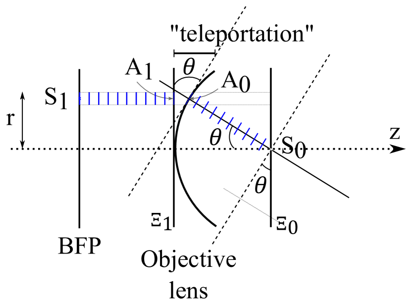
(a)

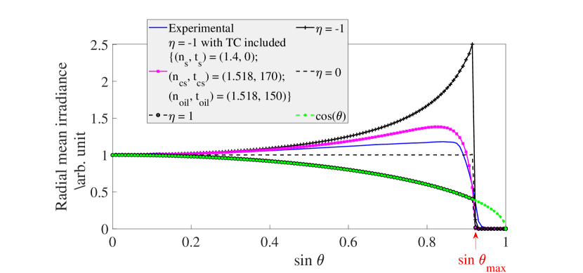
(b)

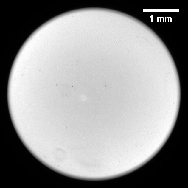
(c)

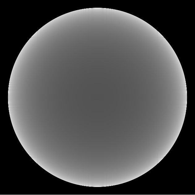
(d)

(e)

(f)

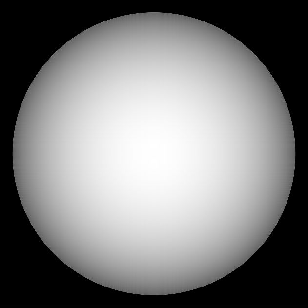
(g)

Figure 5: Aplanatic correction for energy conservation. (a) Schematics illustrating the “aplanatism effect”. (b) Radial mean of the normalized BFP intensities. The normalization is done in such a way that the power remains constant. We have here the image of the BFP (c) recorded experimentally using a $70$ $\mathrm{n}\mathrm{m}$ microtom-sectioned thin layer of fluorescent Chroma slide attached to the coverslip and embedded in immersion oil. Figure (c) is cropped from the original experimental BFP image for display. The corresponding BFP computed theoretically use different scaling factors $\sqrt{\cos^{\text{$\eta$}}(\theta)}$ of the electric field. (d) $\eta$ = $-1$, (e) $\eta$ = $-1$ and included transmission coefficients (TC) due to the layer system {sample of refractive index $n_{s}$ placed exactly at the surface of the coverslip, coverslip of refractive index $n_{cs}$ and thickness $t_{cs}$, oil immersion of refractive index $n_{oil}$ and thickness $t_{oil}$ }. The thicknesses of each layers are expressed in $\mathrm{\SIUnitSymbolMicro m}$ and are assumed to be the same as in the design condition of the system. (f) $\eta$ = $0$ and (g) $\eta$ = $1$.

In a system where the equivalent refractive locus corresponds to a Gaussian reference sphere, the system satisfies the Abbe's sine condition. The energy conservation yields to the notion of an apodization or aplanatic factor (AF), which is equal to $\sqrt{cos(\theta)}$ (Sheppard and Gu, 1993).

The concept can also be understood by using a simple geometric figure (see Fig. 5(a)). Firstly, let us assume an isotropic emitter placed at the centre of the Gaussian reference sphere, $S_{0}$. Since the emitter is emitting uniformly in all directions, the strength of the amplitudes on the Gaussian reference sphere is uniform. In Fourier space, the spectrum on the McCutchen pupil is as well uniform. Let us consider a small parallel ray which is redirected from the Gaussian reference sphere at a given angle $\theta$. If we attribute a given irradiance $I_{0}$ as a power $P_{0}$ per unit area $A_{0}$ to such a beamlet from $S_{0}$, the same power will have to be distributed to a smaller area $A_{1}=A_{0}\cos(\theta)$ after the teleportation of the beam from the Gaussian reference sphere to the plane parallel to the pupil plane in the BFP (see Fig. 5(a)). This means that the irradiance measured perpendicular to the local direction of propagation changes to $I_{0}/\cos(\theta)$, and each of the field vectors for this beamlet thus needs to change by $\sqrt{\cos^{-1}(\theta)}$ to be consistent with this intensity change. This factor corresponds to 1/AF. The inverse of this effect, which is spreading irradiance to a larger area, is somewhat akin to what happens to radiative power measured on the surface of the earth during winter. It is sometimes called “natural vignetting”. In this manner, the energy spread over the 2D pupil equals to the energy of a point source over the active Gaussian sphere. This corresponds to the imaging of an emission PSF where we have our emitter placed at the focal position of the objective lens, which is at $S_{0}$ in this illustration. If a large enough magnification is assumed, the vectorial and aplanatic facgtor effects caused by the tube lens can be neglected. To describe the Fourier-transformation of the focussed field in this scalar model, we expect a correspondence to the amplitude on the BFP and therefore a $\sqrt{\cos^{-1}\theta}$ dependence.

To now understand the factor that needs to be applied to conserve the energy when focussing a uniformly illuminated 2D pupil (BFP) with a high-NA objective (excitation PSF), let us consider the same Fig. 5(a). The point $S_{1}$ denotes a point in the BFP from which a ray emerges. $S_{2}$ being the focal point of the objective corresponds to $S_{0}$. We can consider the reciprocity theorem: a lossless (non-magnetic) monochromatic optical system in which a field $(E_{x_{0}},E_{y_{0}},E_{z_{0}})$ (here an isotropic emitter) at position $S_{0}$ gives rise to a field $(E_{x_{1}},E_{y_{1}},E_{z_{1}})$ at position $S_{1}$ in the image plane, warrants that placing the isotropic emitter $(E_{x_{0}},E_{y_{0}},E_{z_{0}})$ as a source at the former image plane, generates the field $(E_{x_{1}},E_{y_{1}},E_{z_{1}})$ at the focus position $S_{0}$ of the objective(Sheppard and Gu, 1993). The latter situation, a uniform emitter at the focus of the tube lens, leads, due to the low NA of the tubelense to the aforementioned uniform illumination of the pupil plane (BFP). Therefore the excitation PSF should be equal to the emission PSF as long as we can neglect the NA of the tubelens. This is confirmed also by considering the $\sqrt{\cos\theta}$ dependence on the Gaussian reference sphere and thus on the McCutchen pupil. To arrive at the 2D Fourier-transform of the in-focus excitation field, we need to project the McCutchen pupil and thus apply the projection factor $cos^{-1}\theta$ which leads to an overall amplitude of $cos^{-1}\theta\sqrt{\cos\theta}=\sqrt{\cos^{-1}\theta}$ confirming the above reciprocity argument.

III.3.1 Emission PSF

To test the theory described above, we measure experimentally the intensity of the BFP of emitting Flourophores. A large collection of randomly orientated emitters (e.g. fluorescent) quickly rotating emitters will emit with the same intensity along all directions. The detection objective is thus expected to concentrate the light it receives at high angles. This effect is visible when imaging the back focal plane of an objective imaging a fluorescent plane sample of uniform emitters.

In Fig. 5(c), we show the image of the BFP of a high-NA objective imaging a $70\text{\,}\mathrm{nm}$ thick layer of a Chroma slide. For the imaging, we have to take great care with our measurements to avoid supercritical angle fluorescence effect as we did not account for this in our calculation. Fluorophores which are directly at a dielectric surface emit fluorescence into the coverslip and thus the objective with a totally different angular characteristic. This affects the pupil plane distribution and completely changes the expected measured PSF if not corrected appropriately. To avoid this effect, we embedded the thin layer of Chroma slide in oil with refractive index of $1.518$ and place it onto a coverslip. A microscope slide is used to support the sample.

The image of the BFP is recorded by removing the eyepiece through the observation tube of the microscope [Zeiss Axio Observer, Objective Plan-Apochromat $63\times/1.4$ Oil DIC M$27$] and replacing the eyepiece with a system composed of a converging lens of $50\text{\,}\mathrm{mm}$ focal length coupled with a Basler camera [acA4024-$29$um] (see Fig. 6). The Basler camera is placed at $50\text{\,}\mathrm{mm}$ after the lens. An x-cite lamp is used as illumination light source for this particular measurement. Due to missing information on the optics inside the microscope observation unit, we were not able to determine the theoretical magnification of our pupil plane re-imaging but estimate it to be 0.446 as given by the ratio of the measured over the theoretical pupil radius. The pixel size of the recorded BFP is estimated to be $4.148\text{\,}\mathrm{\SIUnitSymbolMicro m}$. The pupil diameter is calculated to be $4.816\text{\,}\mathrm{mm}$ and is represented by $1160\text{\,}\mathrm{p}\mathrm{i}\mathrm{x}\mathrm{e}\mathrm{l}\mathrm{s}$ on the detector.

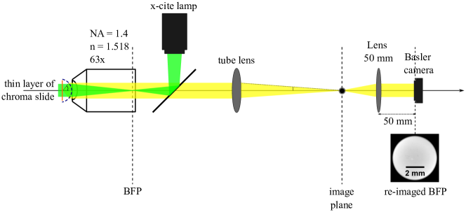
Figure 6: Back focal plane re-imaging system using a thin layer of chroma slide as a sample emitter.

In Fig. 5(b), the radial mean profile of the BFPs is normalized such that the intensity at the angle of incidence equal to $0$ corresponds to $1$.

Theoretical models are calculated using the slice propagation method described in Section IV.2 at higher sampling under different $\eta$ parameter in the amplitude factor $\sqrt{\cos^{\eta}(\theta)}$ . Those models are computed to match the experimental pupil size. In Fig. 5(d), we have the BFP of an emission PSF ($\eta=-1$ thus predicting an intensity scaled by $\cos^{-1}(\theta)$). We observe that the qualitative expectation (an increase towards the edge of the pupil) is experimentally confirmed but the theory predicts a stronger rise of intensity with $\theta$ than was experimentally found.

This difference could be caused by the photoselection of preferably in-plane transition-dipoles which leads to a less pronounced emission along $E_{z}$ components and thus less pronounced higher angle contributions. The experiments should be repeated with a thin volume of freely rotating dipoles with a rotational correlation time far below the fluorescence lifetime. A further effect could be due to residual back-reflections at higher angles effectively dimming the light at high angles.

To have a realistic model to compare with the experimental result, we use the theoretical BFP with $\eta=-1$ and include the transmission coefficient (TC) due to refractive mismatch of different layers (see Fig. 5(e)). The TC is calculated using Eq. (17) in (Török and Varga, 1997). We assumed the 70 nm thick polymer sample matrix having a refractive index of $1.4$ placed at the surface of the coverslip. For the coverslip we assumed a $170\text{\,}\mathrm{\SIUnitSymbolMicro m}$ thick glass with a refractive index matching the immersion oil $1.518$. We observe in Fig. 5(b) the radial profiles of each of the BFP models. It may also be worth considering that the spectrum of fluorescence emission from the thin slab of fluorescent plastic is a band rather than a single wavelength (Kubitscheck, 2017), but we did not consider this any further. These preliminary experiments qualitatively confirmed the model of the aplanatic factor. As a result, high angular amplitudes in detection get enhanced by $\sqrt{\cos^{-1}(\theta)}$.

III.3.2 Intensity

As a matter of perspective, if our interest resides in calculating a three-dimensional intensity distribution defining the rate at which randomly oriented molecules will be excited, the scaling factor ($\sqrt{\cos^{-1}(\theta)}$ in the Fourier transform of the amplitude in the focal plane) described in the previous section should yield the correct values. The randomly oriented fluorophores have on average the same probability of excitation independent of the angle under which the light comes from. Therefore, the excitation probability is proportional to the sum of the absolute squares of all three field components, $E_{x},E_{y}$, and $E_{z}$. This quantity is proportional to the “radiant intensity” measured in steradians per area which is different from the radiant flux (called “irradiance”), which is often called “intensity”. However, the physically relevant quantity can also be irradiance (e.g. when projecting onto a camera) which quantifies the flux through a unit area oriented perpendicular to the optical axis. In this later case, i.e measuring the focal intensity with a pixelated detector, we would need to account for another Lambertian factor ($\cos^{2}(\theta)$ for intensity or $\cos(\theta)$ for amplitude) in addition to the aforementioned factor (see Fig. 5(a)).

III.4 Sampling condition

The imaging of a PSF, which is ultimately detected on a pixelated imaging device, can commonly be done by a CCD or CMOS camera. Those devices integrate, in each of their rectilinearly spaced pixels, over the signal weighted by a pixel sensitivity function. A PSF calculation typically samples the continuous mathematical function at infinitely thin (delta-shaped) points. Luckily the local integration of the PSF in every pixel by the camera can be rewritten as first convolving the PSF with the pixel sensitivity function and then sampling it at regularly spaced points. Due to the convolution theorem, the effect of detector integration can be represented by a simple multiplication of the Fourier transform of the PSF, the optical transfer function (OTF) with the Fourier transform of the pixel sensitivity function. If we assume square pixels with uniform sensitivity, the OTF gets modified by a multiplication with a $\operatorname{sinc}\left(\pi k_{x}/k_{\text{samp}}\right)\operatorname{sinc}\left(\pi k_{y}/k_{\text{samp}}\right)$. This means that at twice the current sampling frequency $k_{\text{samp}}=1/d_{\text{samp}}$ the overall transfer would cross zero, $d_{\text{samp}}$ being the pixel pitch. To sample the PSF free of aliasing, the highest frequency has to be at most at the half of the inverse of the sampling size. This frequency is called the Nyquist frequency, $k_{\text{Nyq}}=k_{\text{samp}}/2$, and the requirement constitutes what is called the Nyquist Shannon theorem (Heintzmann, 2006). If the PSF is not sampled under this requirement, i.e. $d_{\text{samp}}>1/(2k_{\text{Nyq}})$, there is a presence of aliasing in the signal (see Fig. LABEL:fig:sampling_effect_in_real_space) leading not only to a potential loss of signal but also to wrong results at frequencies within the frequency band.

It is worth emphasizing that a PSF with perfect circular symmetry (e.g. using circular or random polarization) gets modified by the pixel sensitivity form factor and loses its symmetry, with decreased sensitivity, especially along the diagonal directions connecting the corners of the pixels.

In a confocal microscope, the detection is performed by an integrating detector. However, the data is typically acquired by integrating in each pixel over the pixel dwell time, with the scan not being stopped. As an effect, the confocal excitation and detection PSFs both are modified by a single-directional $\operatorname{sinc}\left(\pi k_{x}/k_{\text{samp}}\right)$ term if the scanning is performed along $x$.

III.4.1 Resolution limit and Nyquist Shannon theorem

For a wide-field microscope imaging fluorescence, the minimum resolvable spatial structure (periodicity) observed in lateral axis is given by the Abbe diffraction limit $d_{xy}=\lambda_{\text{em}}/(2\text{NA})$, with $\text{NA}=n\sin(\theta)$ the numerical aperture, $\theta$ the angular aperture of the objective, $n$ the refractive index of the medium and $\lambda_{\text{em}}$ the vacuum emission wavelength. Therefore, the maximal in-plane spatial frequency is given by $k_{xy,\text{max}}=2\text{NA}/\lambda_{\text{em}}$ (Heintzmann, 2006). Similarly, the axial limit in real space for a wide-field microscope is given by $d_{z}=\lambda_{\text{em}}/(n(1-\cos(\theta)))$. In our calculations the electric field has to be sampled according to the desired PSF, which is sampled twice as fine as the Nyquist-Shannon theorem would require, since resampling when calculating the intensity was not performed in our calculations. Thus the highest frequency of the intensity result has to be sampled with at least two positions per shortes period that can be transmitted by the system (Heintzmann, 2006). This requires the pupil to fit into half the digital Fourier-space representation such that its autocorrelation (i.e. the incoherent OTF) fits in the digital Fourier space. The maximal pupil radius in Fourier space along $x$ or $y$ should be lower than half the maximally represented frequency along $k_{x}$ or $k_{y}$ in our Fourier-space representation.

III.4.2 The Fourier sampling pitfall

Other potential sources of error that have to be considered in addition to the aforementioned sampling are as follows. A digitization of the usually round pupil in Fourier space as a hard aperture onto a rectilinear grid may induce severe artefacts. We consider a field distribution of a high-NA PSF with numerical aperture NA = $1.4$, refractive index $n=1.518$ and emission wavelength $\lambda_{\text{em}}=580$ $\mathrm{n}\mathrm{m}$. The pupil radius, which also corresponds to the Nyquist frequency, is calculated using the theory stated in the previous section. We denote $R_{\text{max}}$ as this pupil radius. We generate a hard aperture with radius equal to $R_{\text{max}}/8$ and calculate the corresponding field distribution in real space by generating the Fourier transform of the hard aperture. The window size for this first experiment is $128\times 128$ pixels.

For symmetry reasons, a perfect circularly symmetric PSF should expected. In Fig. 7(a), a significant deviation from circular symmetry is clearly visible. By repeating the same calculation for $1024\times 1024$ pixels, the discrepancy is significantly reduced even though it is still not totally spherically symmetric (see Fig. 7(c)). However, calculating on such large grids causes a significantly computational overhead ($0.178$ $\mathrm{s}$ vs $0.037$ $\mathrm{s}$ i.e. more than $4$ times slower) which can be unnecessary as the user may not need quite so many pixels of the PSF far away from its center.

Interpolation in Fourier-space to obtain a better representation of the pupil may be one route to reestablish spherical symmetry. However, this is a tricky business (Yaroslavsky, 1997) and we therefore choose a slightly different route. We calculate the two-dimensional ($2$D) Fourier-transform of the uniform pupil disk, for which the analytical solution in real space is well known: $\text{jinc}(R)=J_{1}(R)/R,J_{1}$ being the Bessel function of the first kind. We therefore obtain an “ideally” representation of a disk in Fourier-space by Fourier-transforming a two-dimensional jinc function. This “interpolated” disk can then be appropriately modified with $k$-space dependent phase and magnitude alterations.

The computation time of the $1024\times 1024$ pixels ideal representation of disk in Fourier-space using the jinc trick is $0.078$ $\mathrm{s}$ on average. The calculation is done with MATLAB R2018a on Windows 10 with Intel(R) Core(TM) i5-6200U CPU @ 2.30 GHz 2.40 GHz.

As the jinc-function possesses first order discontinuities in real space at the border, whos Fourier-transformation causes unwanted high-frequencies (Cao, 2003). To avoid this, the jinc-function was modified at the outer rim by appropriately smoothing the $15\text{\,}\mathrm{\char 37\relax}$ of its edges towards zero (“DampEdge” function in the PSFToolbox Holinirina Dina Miora, Kielhorn, and Heintzmann (2022)).

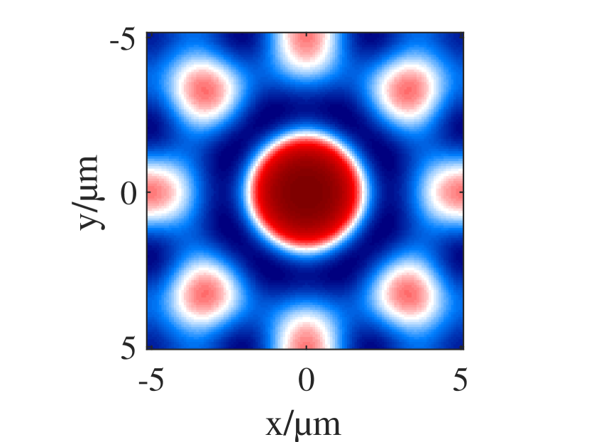
(a)

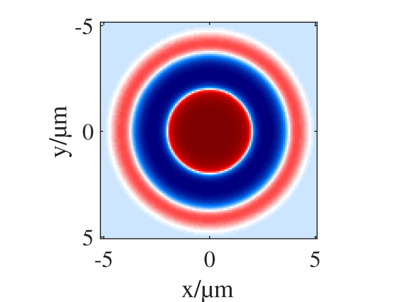
(b)

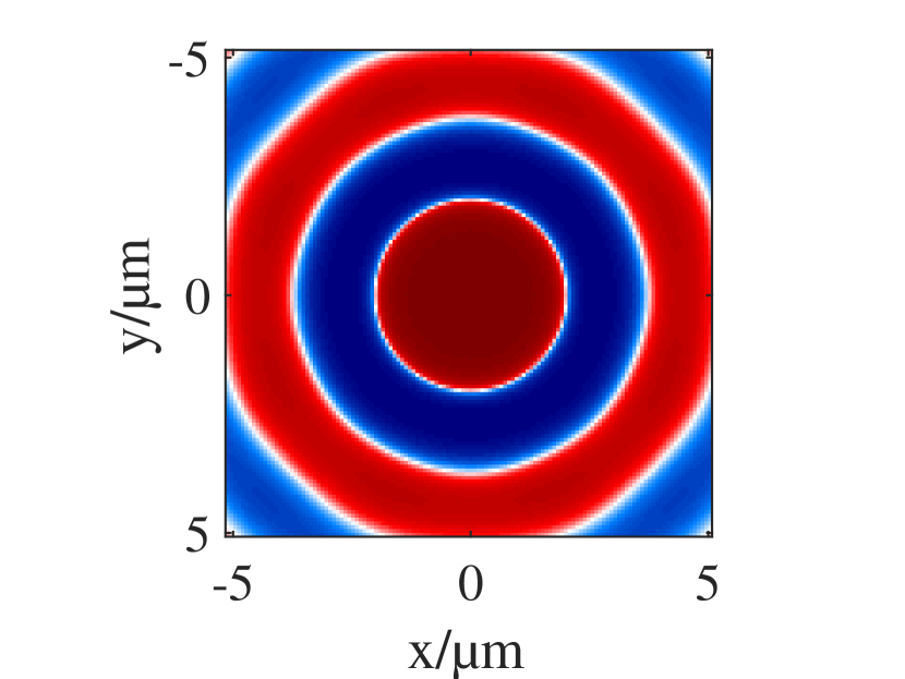
(c)

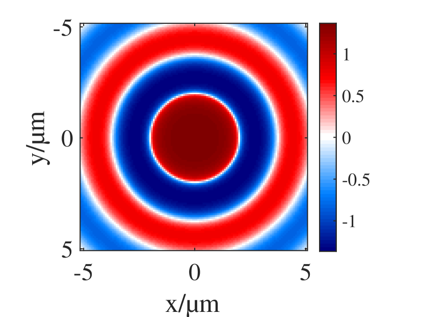
(d)

Figure 7: Field distribution calculated from the Fourier transform of (a) a hard aperture of size $128\times 128$ pixels, (b) a jinc aperture aperture of size $128\times 128$ pixels, (c) a hard aperture of size $1024\times 1024$ pixels cropped to $128\times 128$ pixels size for display and, (d) a jinc aperture aperture of size $1024\times 1024$ pixels cropped to $128\times 128$ pixels size for display. A DampEdge of $15\text{\,}\mathrm{\char 37\relax}$ is applied to the generated field (full size) using the jinc-trick. Figures are displayed at $\tan^{-1}(\gamma E)$ and centered at the zero of the display, $E$ being the field distribution and $\gamma=20$.

As seen in Fig. 7(b), the real-space representation of the field distribution is perfectly symmetric and spherical by design even for images with relatively few pixels. We refer to this method of generating an interpolated disc in Fourier space as the FT(jinc)-pupil trick.

IV Novel Fourier-based methods for PSF calculation

IV.1 The electric field on the $k$-sphere

To calculate the electric field amplitude distribution near the focus, we first need to understand the electric field properties of each Huygens wavelet as previously described. To this aim, we associate each plane wave arriving at the focus with the refractive effect that the “bending” at the Gaussian reference has at the point where this “ray” would hit it. We assume a perfect anti–reflection coated objective lens and all the energy is transmitted for such a ray and exploit the fact that the electrical field of the plane wave needs to be a transversal wave. We thus have to project the electric field at the pupil ($E_{x},E_{y}$) to the electrical field ($E_{x},E_{y},E_{z}$) of the plane waves (i.e. the McCutchen pupil).

Let us consider Fig. 8. The incident wave $\vec{E}_{i}$ is incident from infinity at the left side in Fig. 8 and focuses at a the focal point of the objective lens. The system is assumed to fulfil the Abbe sine condition, requiring the beams to change direction at the Gaussian reference sphere. At the entrance pupil, the incident wave $E_{i}$ can be described by two components ($E_{x},E_{y}$), but it is very useful to here consider a locally varying coordinate system along azimuthal ($\vec{e}_{s}$) and radial ($\vec{e}_{p}$) directions respectively.

Let $\vec{E}_{t}$ denote the field amplitude transmitted along the wave vector $\vec{e}_{t}$ towards a point ($x,y,z$) near the focus where the field is evaluated (see Fig. 8). The unit vector corresponding to the radial component $\vec{e}_{p}$ is refracted by $\theta$ and becomes $\vec{e}_{r}$ while the azimuthal component oriented along $\vec{e}_{s}$ remains unchanged.

$$\vec{e}_{s}=\begin{pmatrix}-\sin\phi\\ \cos\phi\\ 0\end{pmatrix},\quad\vec{e}_{p}=\begin{pmatrix}\cos\phi\\ \sin\phi\\ 0\end{pmatrix}\Rightarrow\vec{e}_{r}=\begin{pmatrix}\cos\phi\cos\theta\\ \sin\phi\cos\theta\\ \sin\theta\end{pmatrix}$$ (5)

The new coordinate system is illustrated in Fig. 8.

(e)

(f)

Figure 8: Schematic diagram of the coordinate systems for the directional change of a scalar wave field $E_{i}$ through an objective lens. (a) Adaptive coordinates on the McCutchen pupil. (b) $2$D pupil plane.

The field amplitude distribution at a point $(x,y,z)$ is therefore given by:

$$\vec{E}_{t}(x,y,z)=(\vec{E}_{i}\cdot\vec{e}_{p})\vec{e}_{r}+(\vec{E}_{i}\cdot\vec{e}_{s})\vec{e}_{s}.$$ (6)

For a given polarization state of the incident wave field $\vec{P}$, the pupil plane amplitude distribution can be calculated using the directional change of the electric field described in the previous paragraphs where the incident electric field is given by $\vec{E}_{i}=E_{0}\vec{P}$, $E_{0}$ is a constant factor which includes the conservation of energy such as aplanatic factor or apodization. Therefore, the amplitude field on the McCutchen pupil is given by

$$\vec{E}_{t}=E_{0}[(\vec{P}\cdot\vec{e}_{P})\vec{e}_{r}+(\vec{P}\cdot\vec{e}_{s})\vec{e}_{s}].$$ (7)

At this point, it seems appropriate to comment on the versatility of this approach. If we want to include any additional linear shift-invariant effect into our calculation, such as the effect of an additional slab of glass, which was not considered in the design of the objective or a wrong medium of sample embedding, it is fairly simple to work out the magnitude, phase and even polarization effect that such a modification would have on each field vector component on the generalized McCutchen pupil.

Likewise, we can also easily consider the effect any intentional change of the complex amplitude transmittance at the pupil plane will have, for example to calculate Bessel beam (McGloin and Dholakia, 2005), spiral phase modification Roider et al. (2014), the doughnut-shaped STED (Stimulated Emission Depletion Microscopy) beam Hell and Wichmann (1994), apodizations (Martinez-Corral et al., 2003) or other PSF modifications (Backer and Moerner, 2014).

IV.2 The slice propagation method (SP)

With the various considerations described above, the complete problem of calculating the in-focus field distribution for excitation and emission PSFs can also be achieved using a method called the “slice propagation”. This method derives from the vectorial Debye model and the propagation of the field is based on the angular spectrum method (Matsushima and Shimobaba, 2009). The steps to follow are:

1. Choose a $2$D pupil plane amplitude and polarization distribution;

2. Propagate it to the Generalized McCutchen pupil as a projection of a two-dimensional pupil onto three field amplitude components;

3. Apply to each component the same aplanatic factor according to the desired calculation in Section III.3 (excitation or emission PSF, angle-independent flux or flux through a reference surface);

4. Perform a separate two-dimensional inverse Fourier-transformation for each of the three field components to go from the McCutchen pupil to the focal field in real space;

5. Calculate the PSF as a probability of excitation or detection for a collection of a randomly oriented fluorophores, $\text{PSF}(x,y)=E_{x}E_{x}^{*}+E_{y}E_{y}^{*}+E_{z}E_{z}^{*}$, such that each of the field components depends on the spatial $(x,y)$ coordinates.

IV.2.1 Free space propagation of the field

In order to calculate a defocussed PSF or $3$D PSF as a stack of defocussed PSFs, we can modify the slice propagation method by including a defocus phase in the generalized McCutchen pupil. Given the field in the McCutchen pupil as illustrated in Fig. 4, the in-focus lateral field distribution components can be calculated as a projection along $k_{z}$ of the corresponding McCutchen pupil. Each projection corresponds to the $2$D in-focus slice of the $3$D field distribution represented by the $3$D McCutchen pupil. To move to a different $z$ position, the Fourier-shift theorem needs to be applied, which states that a translation by $\Delta z$ in real space corresponds to a multiplication with $\exp(ik_{z}\Delta z)$ in Fourier space (Goodman, 2005). Shifting an $xy$-amplitude by $\Delta z$ thus means:

1. Calculate the $2$D fast Fourier transformation (FFT) from real space to Fourier space of the $2$D pupil plane amplitude distribution or use the already calculated projections of the McCutchen field components from the result of step $3$ above;

2. Project onto the $k$-sphere to obtain the field on the McCutchen pupil;

3. Apply the phase modification;

4. Project back (sum along $k_{z}$) onto the $k_{x}k_{y}$-plane;

5. Inverse Fourier transform to obtain the amplitude at $\Delta z$.

These steps follow the angular spectrum method. Luckily, steps $2$ to $4$ do not actually need to be calculated individually, since each pixel exactly ends up where it was but only having accumulated a phase modification which only depends on $|k_{z}|=\sqrt{k_{0}^{2}-k_{x}^{2}-k_{y}^{2}}$. This well-known phase modification (the homogeneous medium angular spectrum “propagator”) can thus simply be applied to the projected McCutchen pupil(s) yielding the wanted defocus PSF in step $5$. When propagating a pupil that was generated by the jinc-FT pupil trick (see Section III.4.2), it is recommended for accuracy reasons not to apply the pupil a second time during propagation.

IV.2.2 Fourier wrap-around pitfall

Even though the propagator with the slice propagation method allows a convenient calculation of the three-dimensional PSF, a severe problem arises outside a $\Delta z$-range in the $xy$-cut through a calculated PSF. The $\Delta z$-range is defined as the axial region where the disk of defocus stays well within the available lateral space provided by the real-space grid (see Fig. 9(a)). Outside the $\Delta z$-range, waves leaving on one side of the $xy-$sampling grid and entering into the simulation from the opposite side due to the periodic boundary conditions of the Fourier-transform cause severe standing–wave effects (see Fig. 9(a) and 9(d)). Three possible strategies can help to avoid this:

1. By appropriately zero-padding the in-focus plane, the $\Delta z$-range from whereon the standing wave patterns occur can be extended (Fig. 9(b)) and 9(e). However, this approach is computationally expensive, since twice the initial image window size slows the calculation down by a factor of $5$. However, padding with zero to twice the original size can still yield unacceptable artifacts for typical $z$ ranges used in $3$D PSF calculations.

2. Establishing absorptive boundary conditions: At every propagated slice, one can apply an ideal absorptive boundary condition to the outside boundary and continue propagation by re-projecting this filtered field onto the pupil plane. This has the disadvantage of sacrificing a good PSF for a portion of pixels near the $xy$ sides of the calculation. In addition, every slice propagation requires two Fourier transformations, instead of only one.

3. Using the chirp Z-transform (CZT). With the help of the CZT, also called zoomed Fourier transform (Rabiner, Schafer, and Rader, 1969) it is possible to calculate only a part of the field without the need for periodic boundary conditions (Fig. 9(c) and 9(f)). In this way the wrap-around artefacts can be partially avoided at the expense of a roughly twice or more increase of computation time.

Practically method C. seems to be the most appropriate among the three options here. The use of CZT for Fourier optics and PSF modelling is not new in the literature and has been proven to be more efficient without loss of accuracy than FFT Leutenegger et al. (2006); Bakx (2002); Smith et al. (2016).

To demonstrate this, the $xz$-profiles of the lower part of the PSFs which corresponds to the slice propagation method using FFT, by zero-padding as described previously as case A and using the CZT as described as case C are displayed at gamma $0.05$ in Fig. 9(d), 9(e) an 9(f) respectively.

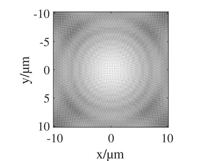
(a)

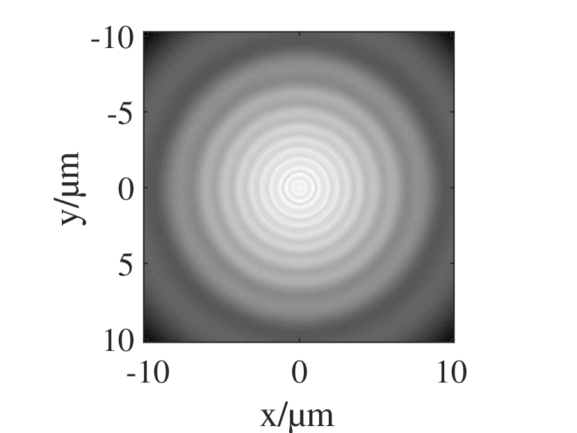
(b)

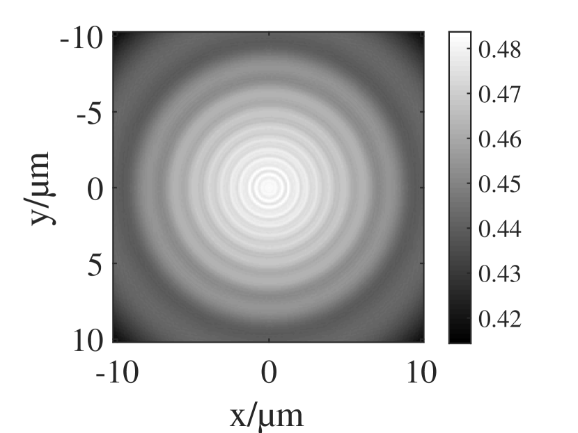
(c)

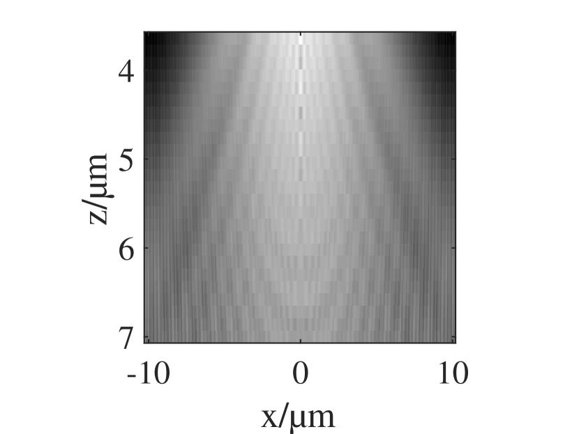
(d)

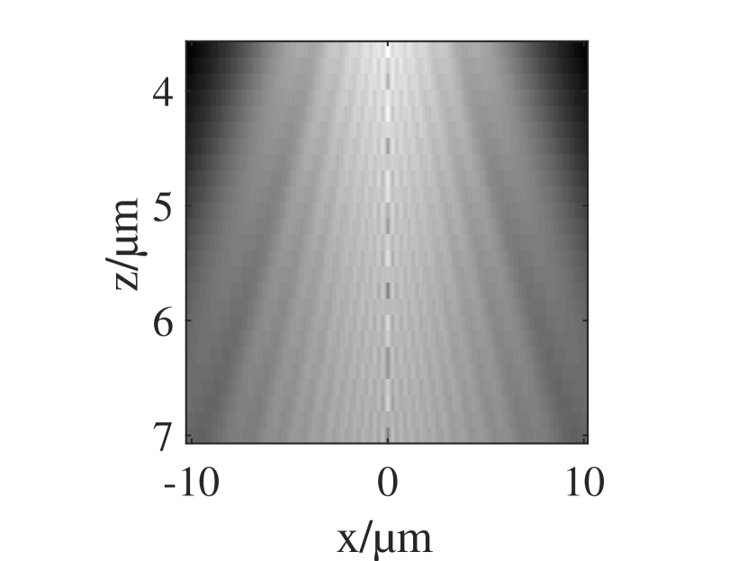
(e)

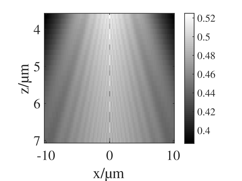
(f)

Figure 9: Profiles displayed at gamma $0.05$ of the PSFs calculated from the slice propagation method. (a, b, c) $xy$-plane at defocus position $7\text{\,}\mathrm{\SIUnitSymbolMicro m}$. (d, e, f) $xz$-cut including to the optical axis starting at $3.5\text{\,}\mathrm{\SIUnitSymbolMicro m}$ away from the focus and with $\Delta z=$ $3.5\text{\,}\mathrm{\SIUnitSymbolMicro m}$. (a, d) Using the standard FFT. (b, e) By zero-padding the image window size to twice. (c, f) Using CZT. The parameters are NA = $1.4$, immersion medium : water ($n=1.33$), polarization : circular; emission wavelength $\lambda_{\text{em}}=$ $580\text{\,}\mathrm{nm}$, voxel size $80\text{\,}\mathrm{nm}$ $\times$ $80\text{\,}\mathrm{nm}$ $\times$ $140\text{\,}\mathrm{nm}$ and, window size : $256\times 256\times 25$ pixel.

The standing waves in Fig. 9(d) and clearly seen in Fig. 9(a) are due to the Fourier-wrap around. These effects are reduced considerably as the window size is doubled (see Fig. 9(b)). A detail comparison of the slice propagation techniques with FFT and CZT with a chosen gold standard is shown in Section V.

IV.2.3 Chirp Z transform

The chirp Z transform (CZT) is a more generalized function converting a signal in real space into a frequency-domain representation. For a $1$D signal $X_{n},n\in[0,N-1]\cap\mathbb{N}$ with $N$ being the number of points of the signal and $\mathbb{N}$ the set of natural numbers, the Z transform $\tilde{X}_{z},z\in\mathbb{C}$ is given as follows:

$$\tilde{X}_{z_{m}}=\text{CZT}(X_{n})=\sum_{n=0}^{N-1}X_{n}Z_{m}^{-n},$$ (8)

where $Z_{m}=AW^{-m},m\in\mathbb{N}$ is a spiral path in $Z-$path with $A$ being the starting point and $W=\exp(-i\Delta\beta)$ the ratio of two consecutive points with a given angular increment phase $\Delta\beta$. For $A=1$ and $\Delta\beta=2\pi m/N,Z_{m}$ is computed over an unit circle and the CZT operation becomes a discrete FFT. To zoom the signal $X_{n}$ in by a scalar factor $c$, $A=\exp(-i\pi/c)$ and $W=\exp(-i2\pi/Nc)$ (Rabiner, Schafer, and Rader, 1969). Therefore, Eq. 8 can be expressed in terms of convolution as follows (Leutenegger et al., 2006):

$$\tilde{X}_{z_{m}}=W^{m^{2}/2}\text{FFT}^{-1}\left(\text{FFT}\left(X_{n}A^{-n}W^{n^{2}/2}\right)\cdot\text{FFT}\left(W^{n^{2}/2}\right)\right).$$ (9)

The inverse CZT of a signal $\tilde{X}_{z_{m}}$ in a frequency-domain representation is defined as the complex conjugate of the CZT of the complex conjugate $\tilde{X}_{z_{m}}^{*}$ of $\tilde{X}_{z_{m}}$ within some scaling factor for a CZT operating on a unit circle (Frickey, 1995). The propagator function using CZT is:

1. Calculate an appropriate zoom-in factor $c$ such that the lateral window size of the calculated PSF is slightly bigger or equal to the lateral dimension of the PSF at the position $\Delta z$ from the focus. The factor $c$ is calculated as $c=(D+N_{xy}/2)/(N_{xy}/2)$, where $\tan\theta_{\text{max}}=D/\Delta z$ in real space and $\tan\theta_{\text{max}}=k_{xy}/k_{z}$ in Fourier space with $\theta_{\text{max}}$ being the maximal angular aperture and $N_{xy}$ the number of pixels in the $xy$-plane (see Fig. 10);

2. Zoom in the pupil plane amplitude distribution with the calculated factor $c$. If the factor $c$ leads to a pupil radius bigger than the given window size, an appropriate new target image size must be chosen, and the pupil radius is always zoomed to just fit in the image window;

3. Apply the angular spectrum propagator (see above)

4. Apply an inverse CZT and zoom out with the same above-mentioned factor $c$ to obtain the amplitude at $\Delta z$;

5. Extract the field within the original window size.

Figure 10: Illustration of the wave propagation in real space for calculating the zoom factor $c$.

IV.3 The sinc-shell method (SR)

This method is based on the fact that the three-dimensional Fourier transform of a complete spherical shell has a convenient solution in real space, which is $\operatorname{sinc}(k_{0}|r|)=\sin(k_{0}|r|)/(k_{0}|r|)$, $k_{0}$ being the wavenumber in the medium and $r$ the radial position. Given this, the sinc-shell method is described as follows:

1. Extend the border of the desired window size N$\times$N by $25\%$ to get a new window N'$\times$N';

2. Generate a $\operatorname{sinc}(k_{0}|r|)$ amplitude distribution in three dimensions in real space within the window size N'$\times$N'$\times z$, $z$ being the range along the axial axis. Multiply this distribution by a compact disk of radius equal to N;

3. Generate a 3D spherical shell by Fourier transforming the result from step 2;

4. Set all values at negative $k_{z}$ to zero (akin to a Hilbert-transform) or and/or keeping only the $k_{z}$-range which contains valid $\vec{k}$ vectors (yielding a change in $z$-sampling and a phase ramp in real space, not affecting intensity values). This half of the 3D spherical shell corresponds to the propagator of the field in free space;

5. Generate $3$ versions (for $E_{x}$, $E_{y}$, $E_{z}$) of the $2$D Pupil as obtained by the jinc-FT trick, each containing the aplanatic factor and the appropriate electric field modification factors.

6. make two additional copies of the 3D McCutchen pupil and apply the $3$ electiv field pupils to each of the $3$ McCutchen spheres by multiplying it with each $k_{z}$ slice. At this point, only a $k_{z}$-range required for the intensity PSF is needed;

7. Perform a three-dimensional Fourier-transformation of each of the three field component McCutchen spheres to obtain the sought-after field components in real space;

8. Extract the field within the desired window N$\times$N$\times z$.

This method has the attractive property that it does not suffer from the Fourier wrap-around effect. The only wrap-around effect is suppressed by extending the window by only $25\%$ and filtering the amplitude field with a disk (step 1 and 2). This filtering in real space corresponds to a convolution of the 3D spherical shell with a Jinc function in Fourier space. It increases the precision in the values of the shell and removes any artefact that may arise during the computation. A disadvantage of this technique is that at least step $2,3$ and $4$ have to be performed while observing the Nyquist sampling along $k_{z}$ for the full field to include its $z$-propagation. This method is also not readily applicable to a single slice (in or out-of-focus).

IV.4 The Fourier-shell interpolation (VS)

This method aims at representing the useful part of the McCutchen pupil directly in $3$D-Fourier-space and projecting the two-dimensional pupil functions onto this three-dimensional shell. The difficulty is that the shell, at each integer $[k_{x},k_{y}]$ position has a non-integer $k_{z}$ position which needs to be represented by interpolating along $k_{z}$ in Fourier space.

As a credible representation of such a non-integer $k_{z}$ would require essentially the whole available $k_{z}$-range, an appropriate compromise to keep the computation efficient was made. We aim to represent only the central part of the corresponding real-space representation as faithfully as possible and label the rest as “don't care” region (see Fig. 11(b)). The border of this “don't care” region is limited by a chosen factor (here it is chosen to be at the $8^{\text{th}}$ pixel from both edges). To calculate the necessary Fourier space interpolation kernel, the part of real space near the border of the z-volume is iteratively updated, while the central part is forced to the expected values in each iteration in this iterative Fourier transformation algorithm (IFTA).

In addition, a pre-defined cut-off frequency is chosen. This cut-off frequency limits the number of interpolation coefficients, which can be used to fill the voxels along $k_{z}$ in Fourier-space adjacent to the one nearest to the non-integer $k_{z}(k_{x},k_{y})$ position of the McCutchen pupil. The cut-off frequency here is set to $\pm 8$ Fourier space pixels yielding $17$ interpolation coefficients to be determined. The required interpolation coefficients are generated with the help of the IFTA (Alsaka, Arpali, and Arpali, 2018). An interpolation table of $60$ sup-pixel positions along $k_{z}$ was pre-computed via IFTA. As initialization, ideal non-cyclic $\exp(2\pi ik_{z}z)$ waves were generated in real space corresponding to the respective sub-pixel frequencies in Fourier space. The ideal waves are then Fourier-transformed and only $N_{z}$ (here $17$) interpolator values are kept and all others are set to zero. The result is transformed back to real space, where the central area (here the inner is about $66\text{\,}\mathrm{\char 37\relax}$ of the given $z$-range) is replaced by the original perfect waves, but the “don't care” region is not touched. This is repeated (typically $500$ times) until convergence. The so-generated interpolation table ($17$ complex valued coefficient as a function of $60$ sub-pixel locations) is stored for later use (see Fig. 11(c)). Note that we only need to calculate the residual non-integer part of an oscillation, leading to an interpolation table which only contains less then one oscillation. The integer oscillations are taken care of by the placement of the kernel in Fourier-space. A typical example for the offset of $0.25\text{\,}\mathrm{p}\mathrm{i}\mathrm{x}\mathrm{e}\mathrm{l}\mathrm{s}$ is shown in real and Fourier space in Fig. 11(b) and 11(d) respectively, overlayed with the ideal subpixel wave (solid line which corresponds to the legend ‘Original signal’). The border of the “don't care region” is indicated by the dashed vertical lines. A real space representation of the full interpolation table is shown in Fig. 11(a) with the “don’t care region” also indicated by the vertical red dashed lines.

The size of the border factor (in pixels) and the cut-off frequency defining the number of interpolation coefficients should be roughly the same. If the “don’t care region” is far bigger than the “do care region”, there tend to be less interpolation coefficients generated for the given region of support frequencies in Fourier space, which is delimited by the blue dashed lines in Fig. 11(c). This leads to a large computational overhead for a given region of interest, since the region requires extensive padding . A small “don’t care region” on the other hand can lead to inaccuracies inside the “do care region” hence the region of support frequencies in Fourier space.

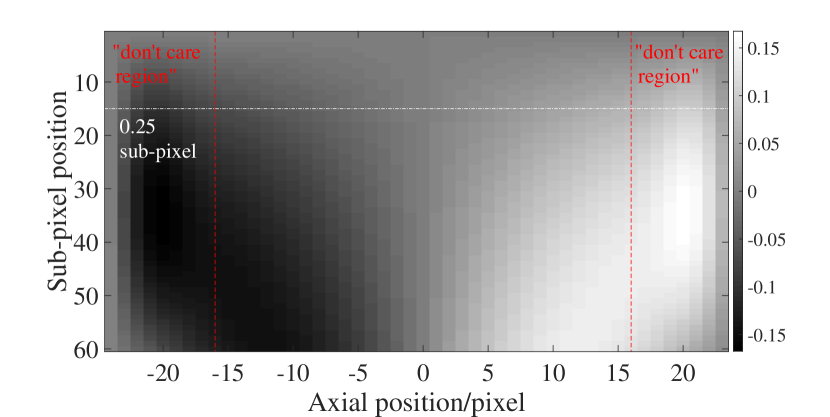
(a)

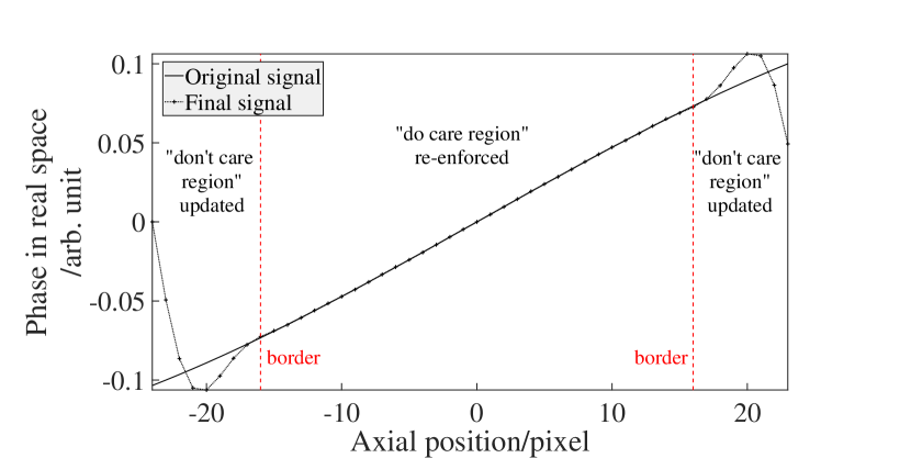
(b)

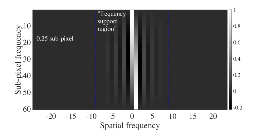
(c)

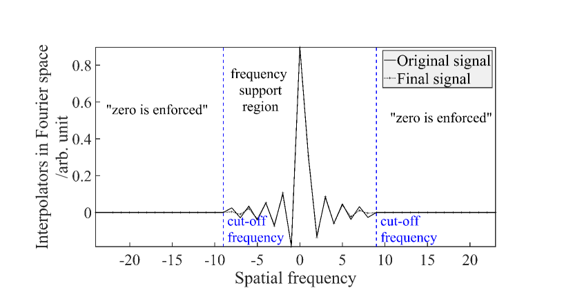
(d)

Figure 11: (a) Phase shift in the ideal wave $\exp(2\pi ik_{z}z)$. (b) Phase at a sub-pixel $0.25$, indicated by the horizontal white line in (a). (c) Interpolation table in Fourier space containing the interpolator coefficients at $60$ different sub-pixels. (d) Interpolation coefficients in Fourier space along the $0.25$ sub-pixel indicated by the horizontal white line in (a) and (c).

This PSF generation algorithm based on Fourier-shell interpolation works as follows:

1. Generate the three two-dimensional McCutchen pupil projections as described above (using the jinc-FT trick as described in Section III.4.2)

2. Calculate $k_{z}(k_{x},k_{y})$ for every pixels within the pupil and round it to the nearest $1/60$ subpixel $k_{z}$ position;

3. Write these pupils into Fourier space by applying the appropriate interpolation kernel for this sub-pixel position;

4. Perform a three-dimensional Fourier transformation to obtain the three-dimensional field distributions (with expected errors in the “don't care region”).

This method can be performed fast and memory efficient as a single access operation in Matlab by exploiting its indexed addressing capabilities. In this way, the complex-valued $2$D pupil can be rapidly filled into the appropriate Fourier space region with the optimized interpolation coefficients as described above and the “don't care” region can be later removed. The required $k_{z}$-range can be kept to a minimum. This method was originally constructed to help with the reconstruction of coherent tomography data, where each entirely different phase projection can then directly written into Fourier-space without the need of a full immediate propagation (e.g. by the slice propagation method) for each projection, which saves an enormous computational overhead.

IV.5 Dipole emission PSF

In reality, a fluorescent emitter can rotate freely at its place or its orientation can be fixed. The PSF of an emitting dipole in the focal plane depends on the polarization of the illumination light and the dipole orientation in space. To describe the dipole emission, let $\vec{\mu}(\theta_{\text{dip}},\phi_{\text{dip}})$ denotes its emission transition dipole moment which is a function of its elevation angle $\theta_{\text{dip}}$ about the optical axis $z$ and azimuthal angle $\phi_{\text{dip}}$ about $x-$axis. The following steps describe how to accommodate a fixed dipole into the PSF calculation:

1. Calculate the field amplitude distribution by taking only the $x-$polarized part at the pupil plane, using the directional field changes as described above and the appropriate aplanatic factor for an emission PSF to obtain the three-dimensional amplitude field $\vec{E}_{1}=[E_{1x},E_{1y},E_{1z}]$ as a function of lateral distance from the optical axis in the image plane;

2. By projecting this amplitude field on the dipole orientation and calculating the absolute square of the scalar product, we obtain the detected intensity $I_{x}=|\vec{E}_{1}\cdot\vec{\mu}|^{2}$ as measured through an analyzer oriented along $x$;

3. Steps $1$ and $2$ can be repeated for a $y-$oriented analyzer yielding $I_{y}$ and the average intensity without analyzer is obtained as the PSF of the dipole emitter:

   $$\text{PSF}_{\text{dip}}=\frac{1}{2}(I_{x}+I_{y}).$$ (10)

To calculate the intensity in the back focal plane of a dipole emitter with a given transition dipole orientation, the same steps as described above are to follow but instead of taking the amplitude field in the image plane, the user is to use the three-dimensional amplitude field in the McCutchen pupil.

If the illumination light is unpolarized or circularly polarized, averaging over all the dipole orientations or over three different perpendicular dipole orientations leads to the same PSF as obtained by calculating a corresponding illumination PSF using circular polarized light, apart from a possible difference in the aplanatic factor. This leads back to the PSF of an isotropic emitter.

$$\text{PSF}_{av}=\frac{1}{4\pi/3}\int_{0}^{2\pi}\int_{0}^{\pi}\text{PSF}_{\text{dip}}\sin\theta_{\text{dip}}d\theta_{\text{dip}}d\phi_{\text{dip}}.$$ (11)

If the illumination light is linearly polarized, averaging over all the dipole orientations does not lead to a symmetric PSF. Further study in polarization in fluorescence microscopy is found in Sheppard and Török (1997).

V Quantitative PSF comparison

The comparison of the models is performed in two steps. The first step consists of comparing the theoretical models with a chosen gold standard (GS) and the second one consists of comparing all the models with experimental data.

We choose an emission PSF according to the RW₀ model (described in Section II.2.2) with a very high sampling as our GS for the theoretical models comparison. The GS is calculated with a sampling of $16\text{\,}\mathrm{nm}$ $\times$ $16\text{\,}\mathrm{nm}$ $\times$ $100\text{\,}\mathrm{nm}$ and window size of $1280\times 1280\times 64$ pixel. The result is subsampled to $80\text{\,}\mathrm{nm}$ $\times$ $80\text{\,}\mathrm{nm}$ $\times$ $100\text{\,}\mathrm{nm}$ by binning groups of five adjacent pixels along $x$ and $y$ to correspond to what we choose as a “normal sampling”. This normal sampling consists of a voxel size of $80\text{\,}\mathrm{nm}$ $\times$ $80\text{\,}\mathrm{nm}$ $\times$ $100\text{\,}\mathrm{nm}$ and image window size $256\times 256\times 64$ pixel.

The $z$-range by which the VS is computed is set to be $1.5\times$ larger than the other models ($96$ vs $64\text{\,}\mathrm{p}\mathrm{i}\mathrm{x}\mathrm{e}\mathrm{l}\mathrm{s}$) to compare only the “do care region” in the quantitative comparison of the PSFs. The computational cost of this enlarged window size ($256\times 256\times 96$) is therefore taken as the computation time for the ($256\times 256\times 64$) PSF for the case of the VS.

We choose simulation parameters corresponding to our experiment. We have an oil immersion objective where the refractive index of the oil is $n=1.518$ and numerical aperture is NA = $1.4$. To mimic randomized dipole orientation, the polarization state is assumed to be circular and the emission wavelength is $\lambda=$ $580\text{\,}\mathrm{nm}$. The PSFs models are implemented and compared in quality and computational speed. The quantitative comparison is done for a single in-focus plane and for the whole volume, excluding $5\text{\,}\mathrm{\char 37\relax}$ on each side near each image border. Each PSF data is normalized as a 3D Volume to yield an integrated intensity of one at the focal plane over the central $90\text{\,}\mathrm{\char 37\relax}$ in $x$ and $y$. The radial mean intensity profile at the focus position for each model is plotted in Fig. 12 in logarithmic scale.

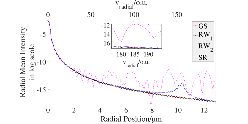
(a)

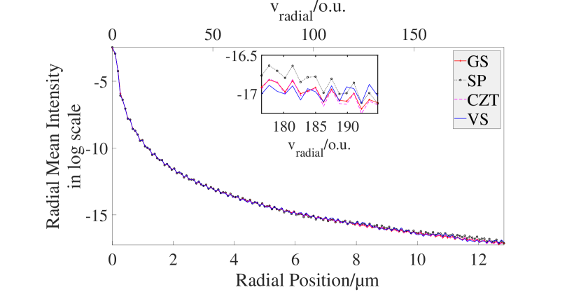
(b)

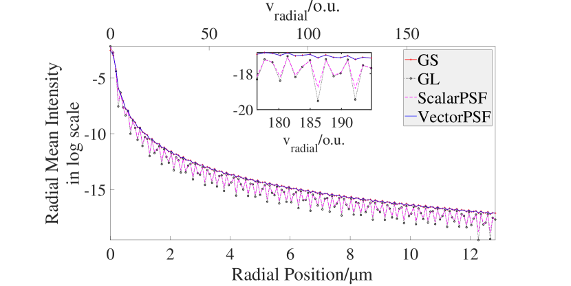
(c)

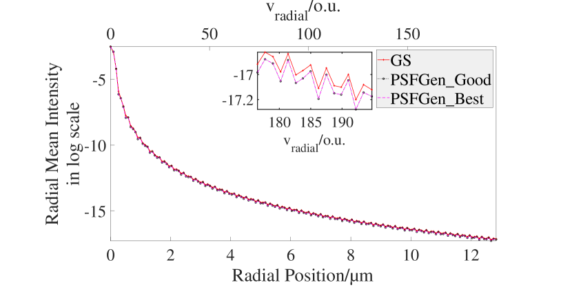
(d)

Figure 12: Radial mean intensity profiles at the focus position in logarithm scale. (a) GS: The gold standard computed using the Richards and Wolf method (Wolf, 1959; Richards and Wolf, 1959), RW₁ and RW₂: two ways for computing the RW models (Section II.2.2), SR: the sinc-shell method (Section IV.3). (b) SP: Slice propagation method with FFT (Section IV.2), CZT: SP technique using the chirp Z transform (Section IV.2.3), VS: Fourier shell interpolation technique (Section IV.4). The state-of-the-art are: (c) A scalar PSF based on the work of Gibson and Lanni (1989) and developed by Li, XUE, and BLU (2017), a scalar and vector PSF from (Aguet et al., 2009) and, (d) a vector PSF calculated with the Richards and Wolf $3$D optical model with good and best accuracy respectively from the PSFGenerator toolbox in (Kirshner et al., 2013). The variable v${}_{\text{radial}}$ denotes the radial optical unit.

In Fig. 12 and the following sections, we denote by RW₁ the RW model calculated by the same technique as the GS but performed at the same (normal) sampling grid as all other techniques (SP, CZT, VS, etc.) to compare to. RW₂ refers to an alternative way for calculating the RW model which uses a Fourier transform along $z$.

V.1 Error analysis and computation time of the theoretical models compared with the RW gold standard (GS)

V.1.1 Model accuracy

To verify how accurate each model is compared to the GS, we use two different techniques: the mean relative error (MRE) and the normalized cross correlation (NCC) between each model and the GS. The MRE has the advantage to describe the average performance-error of each model in comparison with the GS. However, for a data which is shifted and the shifting parameter might be unknown or does not have much importance, the use of normalized cross correlation (NCC) for the comparison is advisable as it is not sensitive to linear shifting. The formula used to compute the MRE is given by

$$\text{MRE(z)}=\frac{\sum_{xy}|GS_{xy}(z)-PSF_{xy}(z)|}{\sum_{xy}|GS_{xy}(z)|}.$$

If not specified otherwise, only intensity values bigger than the $0.1\text{\,}\mathrm{\char 37\relax}$ of the maximum intensity value of GS at each $z-$slice are considered in the calculation of the MRE. The MRE results are displayed in Fig. 13.

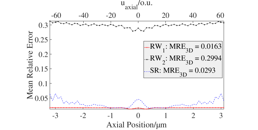
(a)

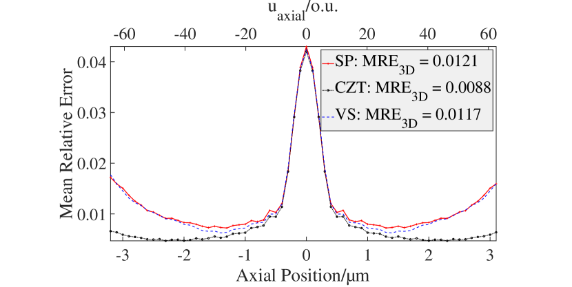
(b)

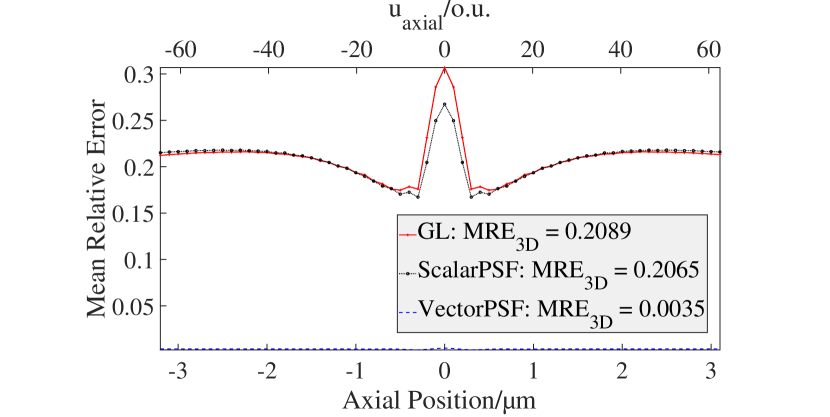
(c)

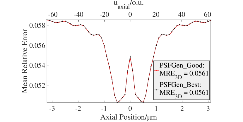
(d)

Figure 13: Mean Relative Error of (a) our RW methods and SR, (b) the SP, CZT and VS and the state-of-the-art (c) GL for the Gibson and Lanni model, ScalarPSF and VectorPSF and (d) vector PSF from PSFGenerator for good and best accuracy with the GS.

We calculate the $2$D NCC slice by slice between our models and the GS. For this, a built-in function normxcorr2 in Matlab is used (MATLAB, 2018). For two $2$D input images, this function generates as an output a $2$D image with double the size minus one of the input images. A value $m$ at a given position $(i,j)$ in the output NCC refers to the NCC of the two images at $(i,j)$ shift. A shift of $(i,j)=(0,0)$ means the two images are on top of each other. The value of $m$ is between $-1$ and $1$, $0$ for zero-correlation, $1$ for maximum correlation and $-1$ for anti-correlation. This technique therefore accounts for possible shifts between the model and the GS. A perfect correlation corresponds to a NCC of $1$ at a shift position $(0,0)$. We report the maximum of the NCC at each $xy$-slice for each axial position $z$ as well as the NCC of the $3$D volume PSF compared with the $3$D GS and have both parameters to check how close the model is to the GS. The result is summarized in Fig. 14.

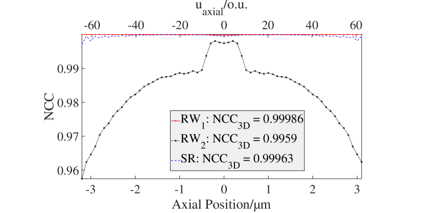
(a)

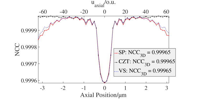
(b)

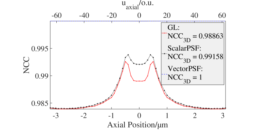
(c)

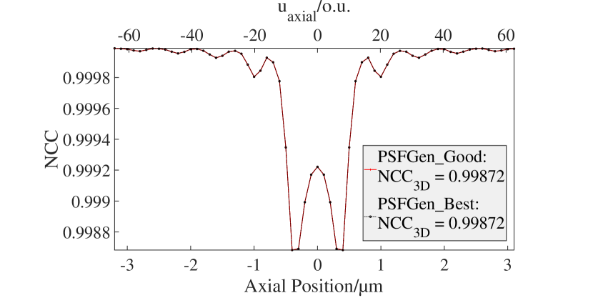
(d)

Figure 14: Normalized cross correlation between the theoretical RW GS with the (a) RW₁, RW₂ and SR methods, (b) the SP, CZT and SR and the state-of-the-art (c) GL for the Gibson and Lanni model, ScalarPSF and VectorPSF and (d) vector PSF from PSFGenerator for good and best accuracy.

V.1.2 The missing cone problem

As observed in Fig. 13 and Fig. 14, the errors between most of the PSF models and the GS are higher at a larger depth and decrease as the field is focusing. The same errors tend to be more enhanced again near the focus. The same observation can be made for the case of the NCC. This observation can be interpreted by studying the missing cone problem of each model.

In wide-field microscopy, the missing cone corresponds to frequencies close to the $k_{z}$-axis that prevent the OTF to transmit information about the object along that axis (Fig. 15(a)). As a consequence, a uniform illumination fluorescence imaging setup is incapable of focussing (or “sectioning”) a planar sample. Out-of-focus light is distributed to different regions but, the energy is still conserved. The integrated intensity at each $z$ position remains the same. This should be the case for any wide-field PSF as long as the PSF remains confined well within the calculation grid. Sufficient sampling turns out to be a key factor, especially for the methods, where radial symmetry is exploited. Since we are dealing with an approximation of the exact field in a finite grid, it is required to have the right amount of data points. An inappropriate choice of grid and pixel size can lead to the violation of the missing cone in the corresponding transfer function of the system. This problem is demonstrated by integrating the PSF for each $xy-$plane at a given axial $z-$position. Even though the radial profile, illustrated in Fig. 12, seems to look good and fits into the GS at the focus position, there may still be significant sampling-related violations of the missing cone. Note that for simulations to accurately evaluate the performance of 3D deconvolution routines on widefield data, preserving the missing cone property is paramount.

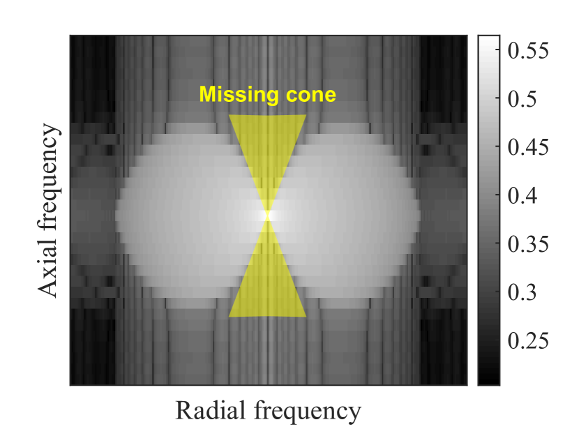
(a)

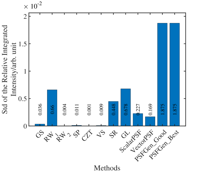
(b)

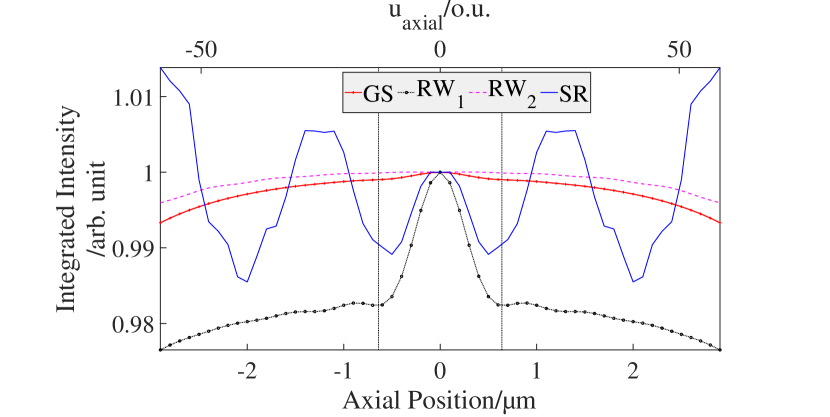
(c)

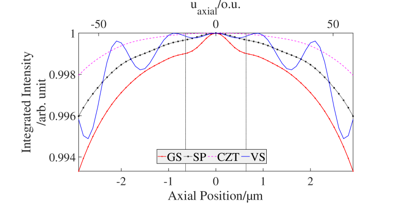
(d)

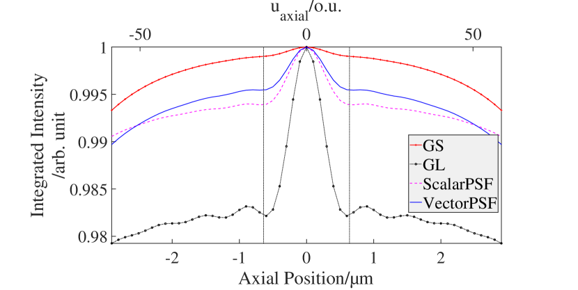
(e)

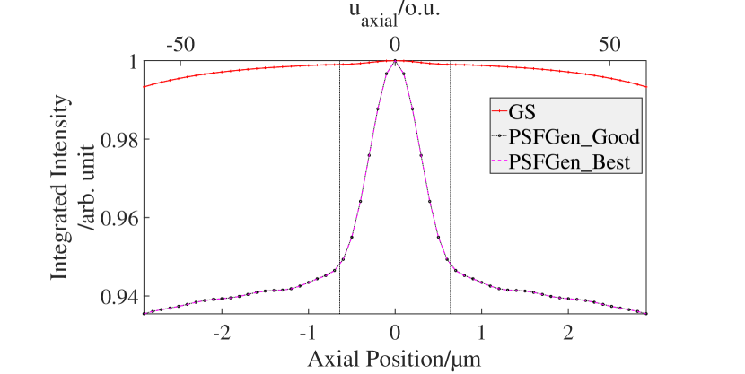
(f)

Figure 15: The violation of the missing cone is observed by calculating the integrated intensity of $90\text{\,}\mathrm{\char 37\relax}$ of the total surface $xy-$plane for each axial position $z$. (a) The OTF calculated from the GS and displayed at gamma of $0.05$. The missing cone is presented in yellow. (b) The standard deviation (Std) of the relative integrated intensity calculated within a $z-$range equal to $1.3\text{\,}\mathrm{\SIUnitSymbolMicro m}$ near the focus. The profiles of the integrated intensity along $z$ from (c) our RW methods and SR, (d) the SP, CZT and VS and the state-of-the-art (e) GL for the Gibson and Lanni model Li, XUE, and BLU (2017), ScalarPSF and VectorPSF (Aguet et al., 2009) and (f) vector PSF from PSFGenerator for good and best accuracy (Kirshner et al., 2013). The variable u${}_{\text{axial}}$ denotes the axial optical unit.

A more precise observation of the violation of the missing cone can be made by zooming on the $z-$range around the focus and displaying the integrated intensity of each slice along the axial position $z$ (see Fig. 15). To quantify this effect, the standard deviation (Std) of the integrated intensities within $20\text{\,}\mathrm{\char 37\relax}$ around the focus of the given $z-$range is calculated and is plotted in Fig. 15(b). This $20\text{\,}\mathrm{\char 37\relax}$ region is delimited by the two dashed vertical lines in Fig. 15(c), 15(d), 15(e) and 15(f). The Std measures the non-uniformity of the laterally integrated intensity over axial position and the importance of the peak of the integrated intensity compared to the minimum within the $z$-range that is considered. The order of magnitude of the Std from the techniques CZT, RW₂, VS, and, SP are in range of $10^{-4}$ which are fairly small and smaller than the Std of the defined GS itself. Increasing the sampling of the models reduce the violation of the missing cone considerably. This is seen in Fig. 15(b) for the case of the GS and RW₁ where the two PSFs are both generated from the same model but with different sampling and window size. The Std has decreased by about $5.41\text{\,}\mathrm{\char 37\relax}$ by oversampling the lateral grid five times. However, higher sampling, i.e. finer step with a big windows, may lead to an expensive computation (about 7$\times$ slower) and requires a larger computer memory.

V.1.3 Wrap-around effect

In addition to the missing cone problem, the wrap-around effect due to FFT-based convolutions can contribute to the accuracy of the model. To investigate this effect, we define a reference window grid $W_{\text{ref}}$ where this wrap-around effect should be minimal. The size of the window $W_{\text{ref}}$ is defined such that the width of the PSF at the highest depth could still fit into it. It is calculated to be:

$$W_{\text{ref}|x}=2\times 2\times\left(\frac{z_{\text{max}}\frac{k_{x|\text{max}}}{k_{z|\text{max}}}+1.3d_{\text{res}}}{s_{x}}\right);$$ (12)

where the first applied factor $2$ is to double the half window; the second factor $2$ is to sample the frequency space two times finer; $z_{\text{max}}$ is the maximum depth expressed in nm; $k_{x|\text{max}}$ and $k_{z|\text{max}}$ are the maximal radial and axial frequency respectively; $d_{\text{res}}$ is the resolution limit of the optical system; the factor $1.3$ is an heuristic factor and, $s_{x}$ is the sampling size along $x$, expressed in nm. The same formulation applies along $y$.

To quantify the wrap-around effect, we generate different PSFs from each model at different windows denoted by $W$ and denote the PSF $h$. We denote $h_{0}$ the reference PSF which is calculated with the reference window $W_{\text{ref}}$. If $W$ is smaller than $W_{\text{ref}}$, the wrap-around effect in $h$ relative to $h_{0}$ is calculated within the window $W$. If $W$ is bigger than $W_{\text{ref}}$, no wrap-around effect is expected. However, the energy is spread over a larger grid so the difference between $h$ and $h_{0}$ is not expected to be zero but is expected to converge to a constant. In this case, we calculate the difference between $h$ and $h_{0}$ within the window $W_{\text{ref}}$. The three-dimensional MRE and mean square error (MSE) between $h$ and $h_{0}$ for the given window for each model are calculated and plotted in Fig. 16.

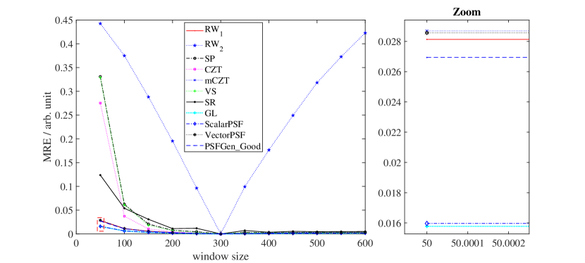
(a)

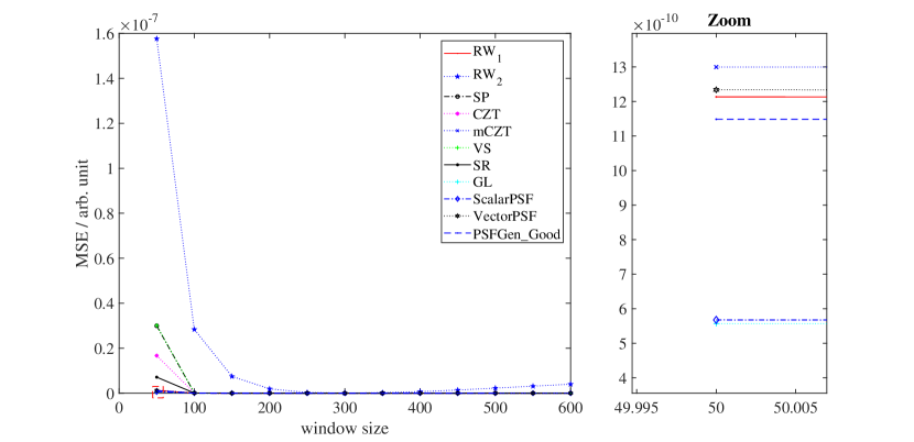
(b)

Figure 16: Quantification of the wrap-around effect in each of the models. (a) Three-Dimensional Mean Relative error. (b) Three-Dimensional Mean Square Error. The right hand side windows entitled Zoom of (a) and (b) are the zoomed-view of the red dashed rectangular in the left hand side.

In this computation, $W_{\text{ref}}$ is calculated and rounded to be $300\times 300$ pixel. The lateral window is square and the rest of the parameters for the comparison are the same as those described for calculating the model accuracy (see Section V).

As mentioned earlier, the scalar PSF based on Gibson and Lanni denoted by GL in Fig. 16 uses Bessel series as a fast approach to calculate the PSF (Li, XUE, and BLU, 2017). As described in (Aguet et al., 2009), a numerical integration based on Simpson’s rule is used to compute ScalarPSF and the VectorPSF. Thus, those models do not possess any FFT wrap-around effect in their computation. They can therefore be used as reference to measure the wrap-around effect.

A modified CZT PSF model, denoted by mCZT, is introduced in this particular PSFs comparison. This model works similarly as the CZT PSF model except the fact that if the given window $W$ as described above is smaller than $W_{\text{ref}}$, mCZT chooses $W_{\text{ref}}$ as window grid for the computation, crops the generated PSF to get the input size $W$ and scale the PSF by the integrated intensity in focus with a window size $W$. The errors between the PSF $h$ at a window $W$ and the reference PSF $h_{0}$ in this case are small enough but are not zeros.

As it is also observed in Fig. 16(a) and 16(b), errors calculated from the Fourier-based models decrease generally as the window grid becomes bigger except for the case of RW₂. However, as it has been said computation of a PSF at a bigger window grid can lead to an expensive computation and requires a larger computer memory.

The wrap-around effect can also be interpreted as undersampling the phase in Fourier-space, which leads to aliasing effects in real space. Large propagation distances thus lead to more aliasing, particularly for small pupils in Fourier space, i.e. small pixel-sizes.

V.1.4 Computational time

To investigate the computation time of each model, we use MATLAB R2018a under the same operating system stated in Section 1.4.2. We run each model with the regular sampling $80\text{\,}\mathrm{n}\mathrm{m}$ $\times$ $80\text{\,}\mathrm{n}\mathrm{m}$ $\times$ $100\text{\,}\mathrm{n}\mathrm{m}$, the same microscope parameters in the previous section. We choose two different window size $256\times 256\times 32$ and $256\times 256\times 256$ pixel and generate the computation time per voxel of each model. The results are displayed in Fig. 17.

As mentioned previously, eight pixels are added on both borders of the $z$-range ($32$ and $256$) to account for the “don’t care region” in the VS model. The addition of $8\text{\,}\mathrm{p}\mathrm{i}\mathrm{x}\mathrm{e}\mathrm{l}\mathrm{s}$ on both sides of the $z$-range $32\text{\,}\mathrm{p}\mathrm{i}\mathrm{x}\mathrm{e}\mathrm{l}\mathrm{s}$ in the VS slows the computation down by a few milliseconds. The first run of the VS requires more computation time. It can go up to $20\times$ or even slower than the second run. The computation is faster in the second run as the interpolators in the models are stored and used for the next computation if the PSF and imaging parameters remain the same.

The computation time per voxel of a PSF using the CZT technique is considerably higher compared to the other techniques apart from the PSF generated from the PSFGenerator at the best accuracy (Kirshner et al., 2013). This computation cost is explained from the fact that the CZT technique expands the lateral size of the PSF to avoid any FFT-based wrap-around problems if the $z$-range is large (See Section IV.2). As the $z$-range increases, the computation time per voxel of the CZT is growing because a large lateral window is needed. A similar cost must be paid when one requires higher sampling to generate a more accurate model and to reduce as much as possible the missing cone error near the focus and any wrap-around effect.

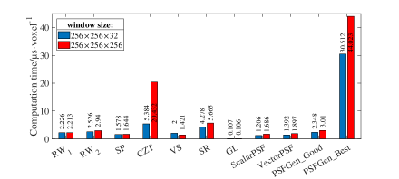
Figure 17: Computational time of each technique per pixel in $\text{\,}\mathrm{\SIUnitSymbolMicro s}$. RW₁ and RW₂ are two ways for computing the Richards and Wolf models (Wolf, 1959; Richards and Wolf, 1959), SP: slice propagation technique (Section IV.2), CZT: SP technique using the chirp Z transform (Section IV.2.3), VS: Fourier shell interpolation technique (Section IV.4), SR: sinc-shell method (Section IV.3), GL: scalar PSF based on the work of Gibson and Lanni (1989) and developed by Li, XUE, and BLU (2017), ScalarPSF and VectorPSF: scalar and vector PSF from (Aguet et al., 2009) and, PSFGen_Good and PSFGen_Best: vector PSFs calculated with the Richards and Wolf $3$D optical model with good and best accuracy respectively from the PSFGenerator toolbox in reference (Kirshner et al., 2013).

V.1.5 Discussion

In summary all the vector models agree closely. VectorPSF has a 3D NCC value equal to 1 while CZT, VS, SP and SR differ deviate at the 4th and PSFGen_Good and PSFGen_Best at the 3rd digit from the perfect NCC of one. The scalar PSFs have the smallest 3D NCC values of 0.9916 for ScalarPSF and 0.9886 for GL.

Similarly, the $3$D mean relative error between the VectorPSF is the closest to the GS with a value of MRE $\approx 0.0035$. This is followed by the CZT model with MRE $\approx 0.0088$, VS and SP models with MRE $\approx 0.012$. This high similarity and accuracy is achieved at a high computation time cost (in average $20.432\text{\,}\mathrm{\SIUnitSymbolMicro}\mathrm{s}\cdot\mathrm{v}\mathrm{o}\mathrm{x}\mathrm{e}\mathrm{l}\,^{-1}$ for the CZT if the window size $256\times 256\times 256$ voxels.

Slightly less accuracy can be achieved for a less expensive computation time with the SP and VS techniques and especially if a repetitive computation of the PSF with the same imaging parameters is required. However, one needs to expand the $z$-range to consider the “don’t care region”. A higher $z$-range is therefore needed accordingly. Another disadvantage of the VS is that the computation of a single slice PSF is not possible with this technique. Similarly, as discussed in Section IV.2.1, SP suffers from a wrap around problem at a higher depth and with a smaller window grid. Nevertheless, SP, CZT and VS are less prone, compared to the other method, to violate the missing cone properties of PSF in wide-field microscopy.

On the other hand, the SR method can beat SP, VS and even CZT in terms of wrap-around effect. The still observed wrap-around effect quantified and displayed in Fig. 16 are due to the jinc aperture added to the pupil aperture stop to limit the field. SR has a very high similarity to the GS especially near the focus. Its missing cone problem is also considerably small but not as small as in SP, VS and CZT. SR is faster to compute than CZT.

PSFGen_Good and PSFGen_Best have relatively higher MRE and lower NCC with the GS compared to the PSF models developed under this project and the state-of-the-art VectorPSF. PSFGen_Good yields to a lower MRE than PSFGen_Best. We speculate that the reason for this could be that the PSFGen_Best is overestimated. The probability to violate the missing cone is higher in the computation of this model. The model is also very expensive in time compared to the other models discussed in this manuscript.

Compared to the rest of the models, the scalar model (GL and ScalarPSF) have the lowest $3$D NCC and highest 3D MRE (after RW₂) with the GS. These values quantify the difference between a vector PSF and scalar PSF. These scalar PSFs are however the fastest models. Their precision and accuracy can be sufficient for some application. Although RW₂ is among the models which have higher ability to satisfy the missing cone properties, its accuracy tends to be close to the scalar PSF models, the least accurate.

V.2 Experimental validation

V.2.1 Experimental PSF data

To validate the model experimentally, a PSF measurement is performed by averaging the images of beads. For this, we use Tetraspeak beads of $100\text{\,}\mathrm{nm}$ in diameter (Invitrogen by Thermo Fisher Scientific, REF T7279). The beads fluoresce with an emission wavelength of $580\text{\,}\mathrm{nm}$ at an excitation light of $561\text{\,}\mathrm{nm}$. The beads are first diluted with distilled water to get $1/400$ concentration and vortexed. We drop some droplets of the solution on a coverslip and let it dry for over $4\text{\,}\mathrm{h}$. Our imaging system is composed of a $63\times$ Zeiss C-Apochromat oil immersion ($n=1.518$) objective lens of 1.4 NA (DIC M27). The choice of the oil immersion for the microscope is very important as this can contribute to any observed aberration in the recorded image. Any contributions from background light is reduced and eliminated during the measurement. The image of background is recorded before any measurement and several measurements are averaged to reduce the noise in the offset estimation. The exposure time of the detector camera is set to be $100\text{\,}\mathrm{ms}$ and the output laser power illuminating the sample is measured at 25 mW.

To obtain the experimental PSF data, an offset image is subtracted from the raw data. The PSF is afterwards constructed by averaging over 64 beads. This averaged PSF data is of size $40\times 40\times 159$ pixel and voxel size $80\text{\,}\mathrm{n}\mathrm{m}$ $\times$ $80\text{\,}\mathrm{n}\mathrm{m}$ $\times$ $50\text{\,}\mathrm{n}\mathrm{m}$. Let $h_{\text{exp }}$denote the experimentally averaged PSF data.

To compare our theoretical models with $h_{\text{exp }}$, two different sets of comparison are conducted. The first set consists of retrieving the phase aberration contained in $h_{\text{exp }}$and add it in the corresponding pupil plane of our theoretical model. This comparison is only achieved with the PSFs in our toolbox (RW₁, RW₂, SP, CZT, VS, SR) since we do not have access to the amplitudes fields of GL, ScalarPSF, VectorPSF, PSFGen_Good and PSFGen_Best. The phase retrieval technique developed by Hanser et al. (Hanser et al., 2004) is conducted to retrieve the pupil function hence phase aberration of $h_{\text{exp }}$. By testing on a theoretically computed known phase aberration and pupil function with the same parameters as the imaging system here, the phase retrieval algorithm is able to retrieve the phase with a MRE of $0.0084\times 10^{-4}$ and the retrieved PSF has a $3$D MRE of $0.786\times 10^{-8}$ compared to the preprocessed measured PSF. Only the $z-$range within the indicated blue dashed in Fig. 18(a) are used for this set of comparison in order to avoid a comparison with only noise. The size of $h_{\text{exp }}$within this region is $40\times 40\times 80$.

The second set of comparison consists of comparing a block region near the focus with higher signal and discard those at higher depth and compare the region with non-aberrant theoretical PSFs.

V.2.2 Theoretical PSF data

The required window to avoid any wrap-around is calculated using Eq. 12. Each theoretical model is computed with a lateral size equal to the result from this computation ($242\times 242$ pixel) and with a depth equal to $80\text{\,}\mathrm{p}\mathrm{i}\mathrm{x}\mathrm{e}\mathrm{l}$. The computed PSFs are cropped to get the same size $40\times 40\times 80$ as $h_{\text{exp }}$. The $xz-$profile can be observed in Fig. 18.

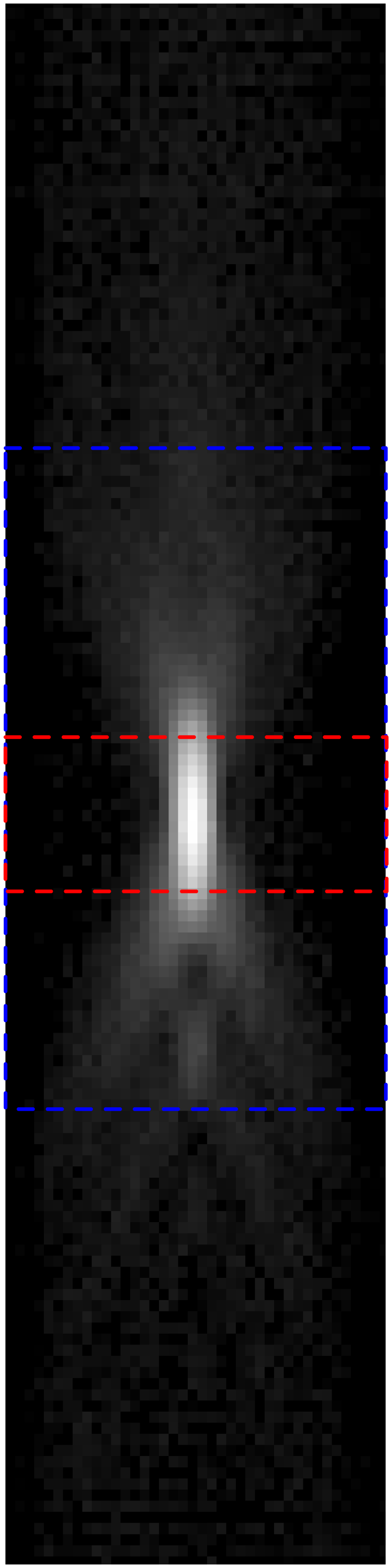
(a)

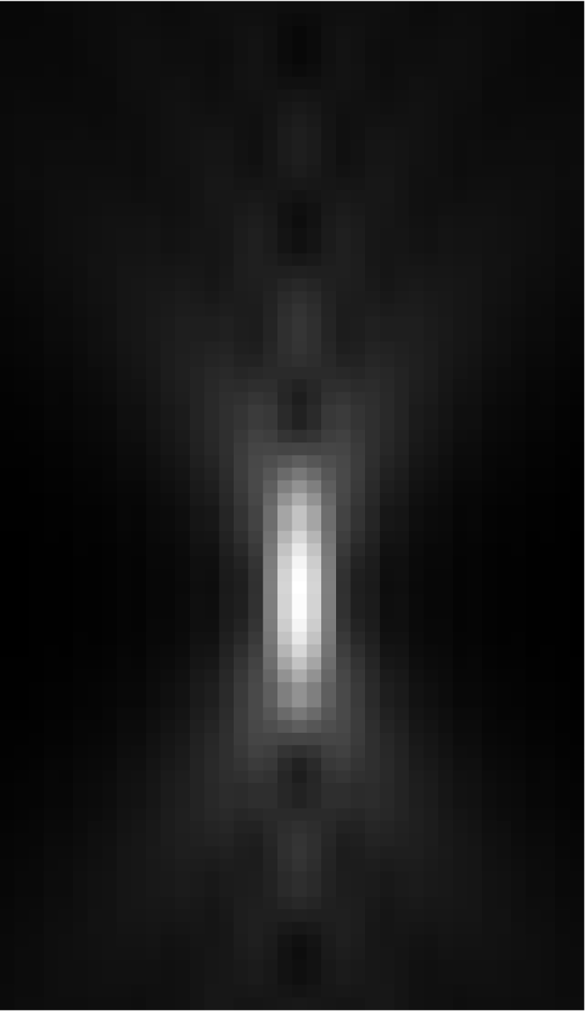
(b)

(c)

(d)

(e)

(f)

(g)

(h)

(i)

(j)

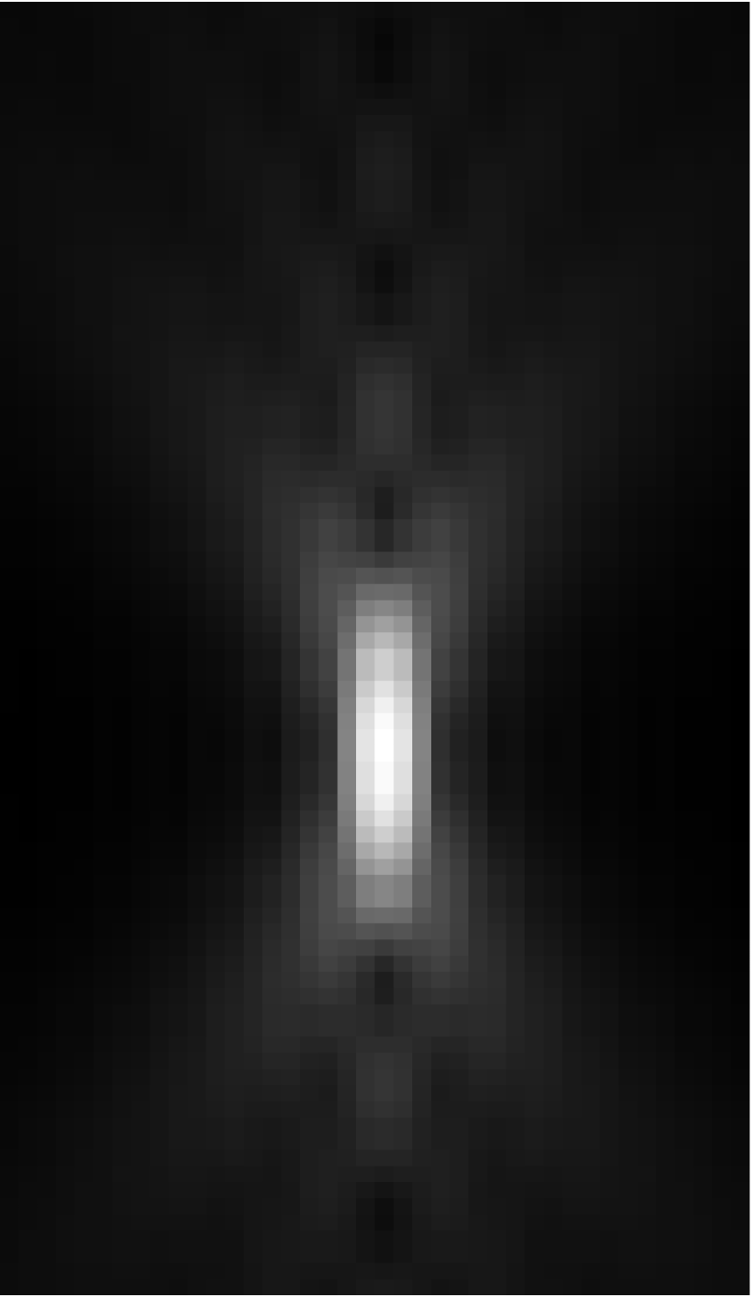
(k)

Figure 18: Meridional sections at gamma $0.05$ of the PSFs of a wide-field microscope with an oil objective of a $1.4$ NA, wavelength emission of $580\text{\,}\mathrm{nm}$, window size $40\times 40\times 80$ and voxel size $80\text{\,}\mathrm{nm}$ $\times$ $80\text{\,}\mathrm{nm}$ $\times$ $50\text{\,}\mathrm{nm}$. (a) Experimental PSF with the blue dashed rectangle indicating the selected region to be the ground truth for the first set PSF comparison and the red dashed rectangle delimiting the ground truth for the second set of PSF comparison. (b) The Richards and Wolf model RW₁. (c) RW₂ using the RW model but computed in different way. (d) SP model. (e) CZT model. (f) Fourier-shell interpolation model (VS). (g) Sinc-shell method (SR). (h) Gibson and Lanni model by Li, XUE, and BLU (2017). (i,j) Scalar and vector models respectively from (Aguet et al., 2009) (k) Vector model using the RW technique computed at the corresponding best accuracy from (Kirshner et al., 2013)

V.2.3 First set of comparison: aberrated PSFs

To retrieve the phase aberration $\Psi$ contained in the averaged experimental data, we take each second axial position of $h_{\text{exp }}$within the blue dashed rectangle indicated in Fig. 18(a). The retrieved phase is displayed in Fig. 19(a). To generate the theoretical aberrant PSFs, the complex-valued amplitude PSFs are $2$D Fourier transformed to obtain their pupil functions and the retrieved phase is added by multiplying the pupil by $\exp^{i\Psi}$. The aberrant pupil is inverse Fourier transformed back to real space and we get the aberrant PSF by taking the absolute square of the aberrant complex-valued amplitude PSFs. The results are displayed in Fig. 19.

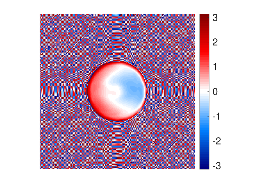
(a)

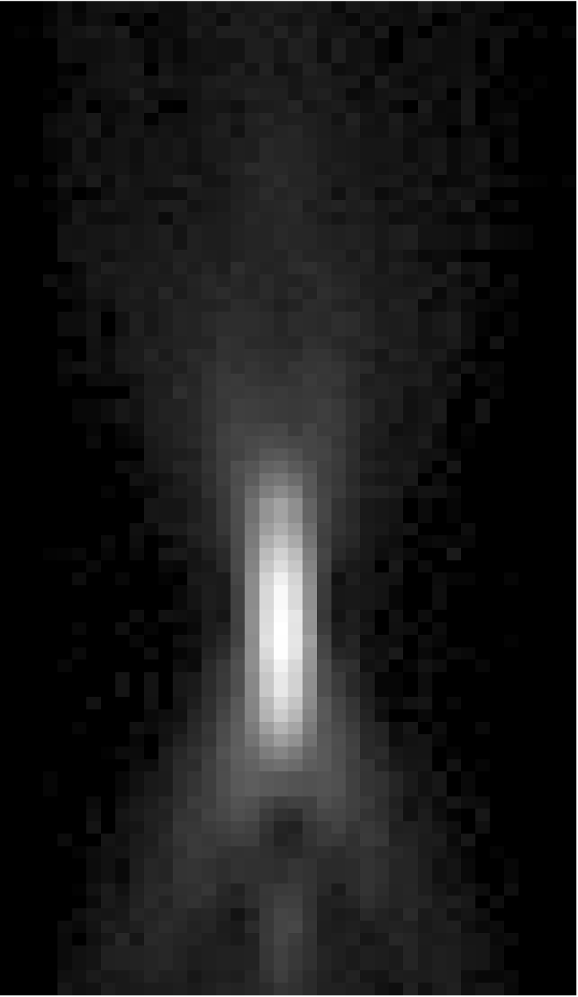
(b)

(c)

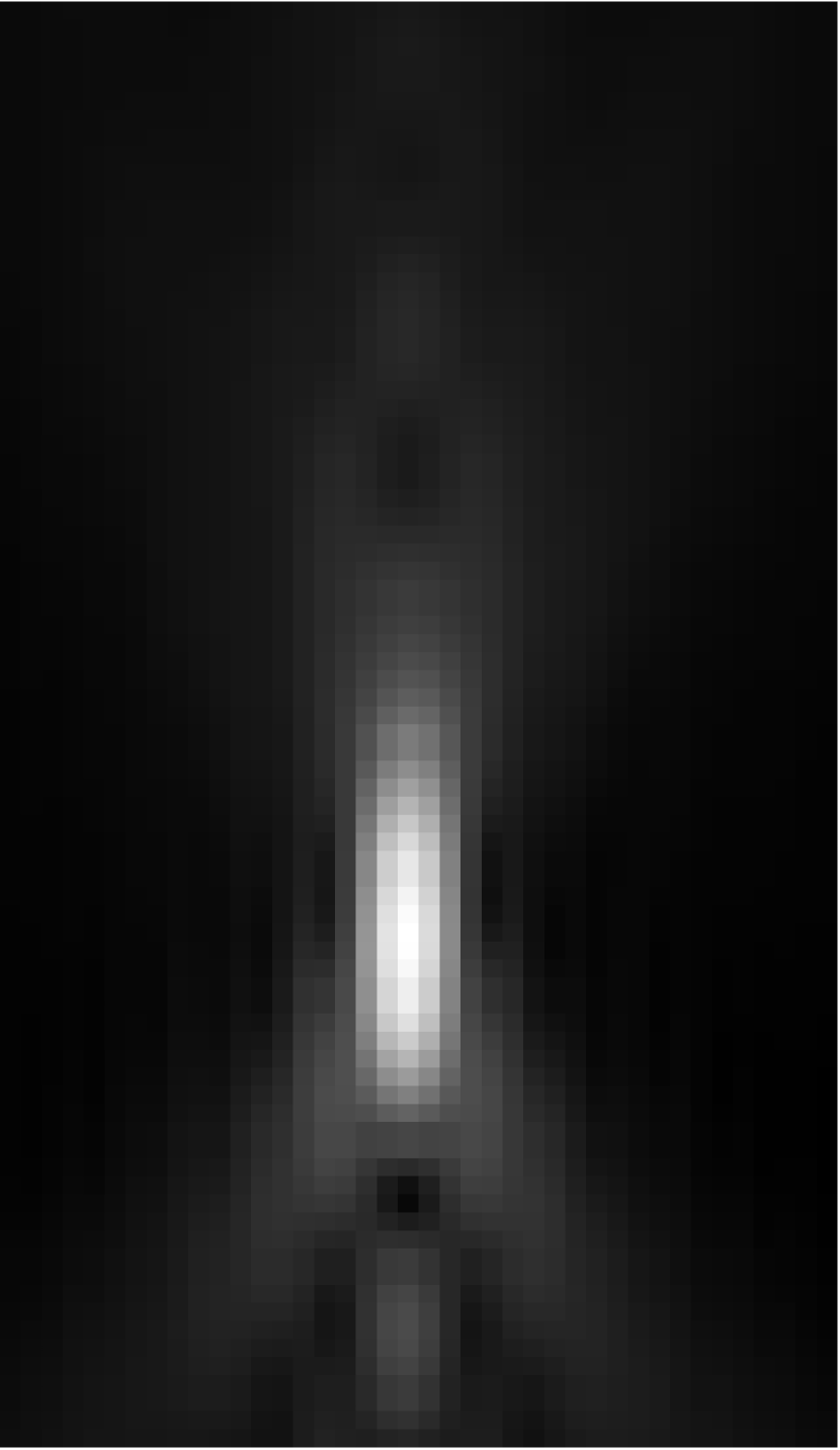
(d)

(e)

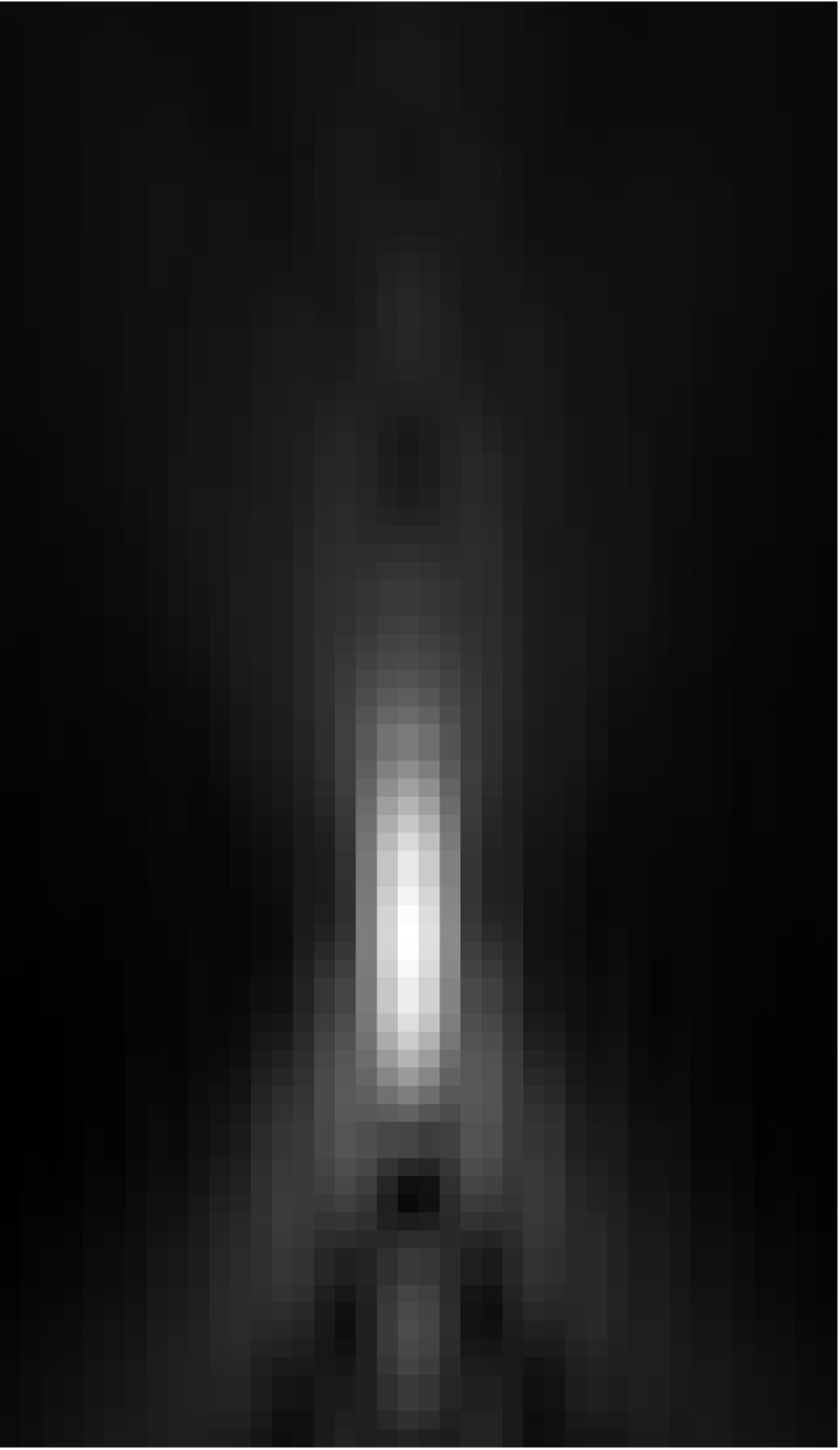
(f)

(g)

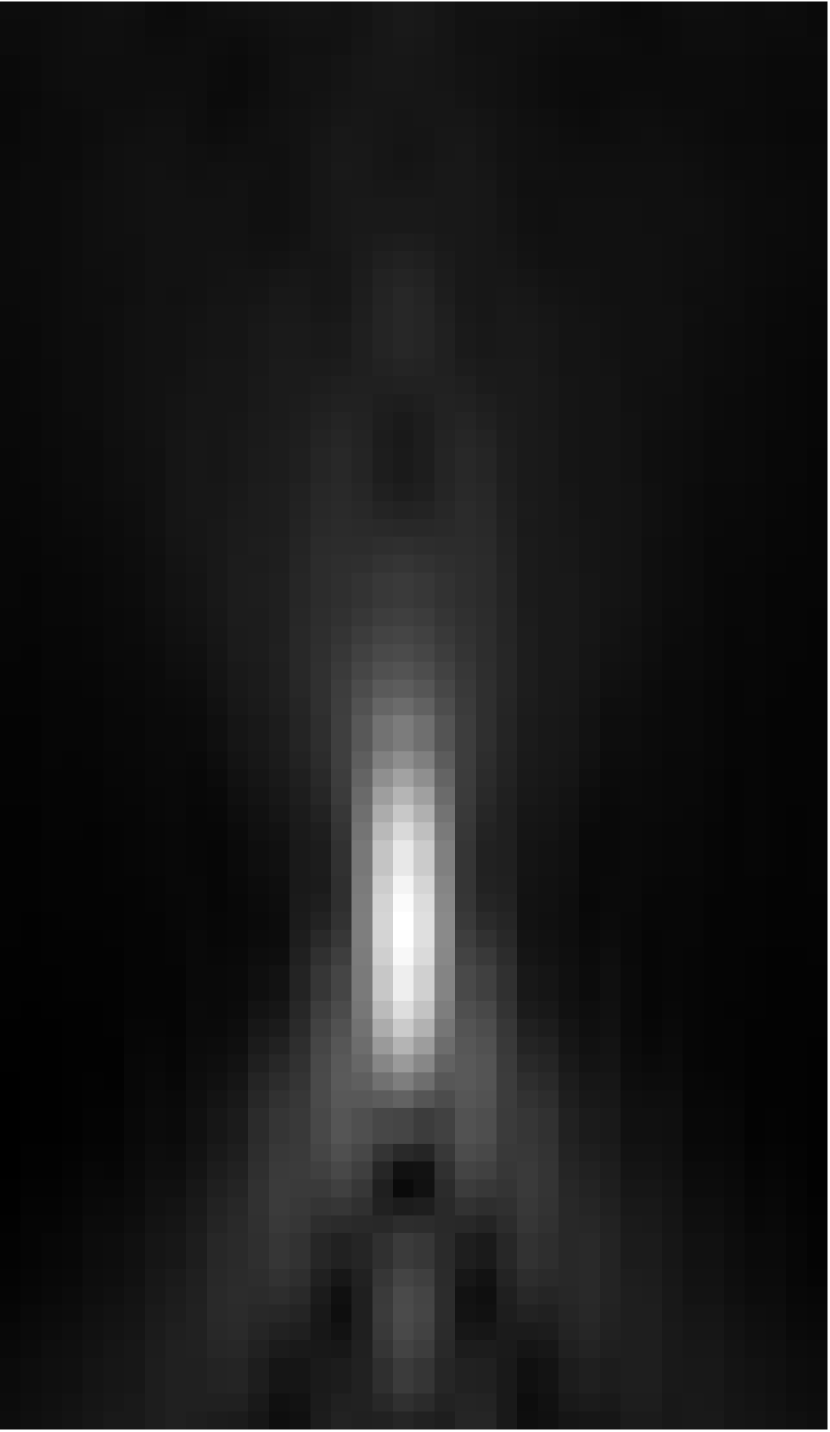
(h)

Figure 19: Comparison of aberrant PSFs with the experimentally averaged PSF data: (a) Retrieved phase aberration from the experimental data; (b) Experimental averaged PSFdata; (c) aberrant RW₁; (d) aberrant RW₂; (e) aberrant SP; (f) aberrant CZT; (g) aberrant VS; (h) aberrant SR. PSFs are displayed at gamma equal to $0.05$.

The similarity and difference between the theoretical aberrant PSFs and $h_{\text{exp }}$are quantified by computing the NCC slice by slice and the MRE respectively. The $2$D NCC results are plotted in Fig. 20(a).

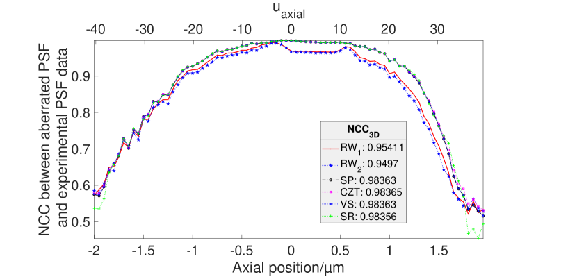
(a)

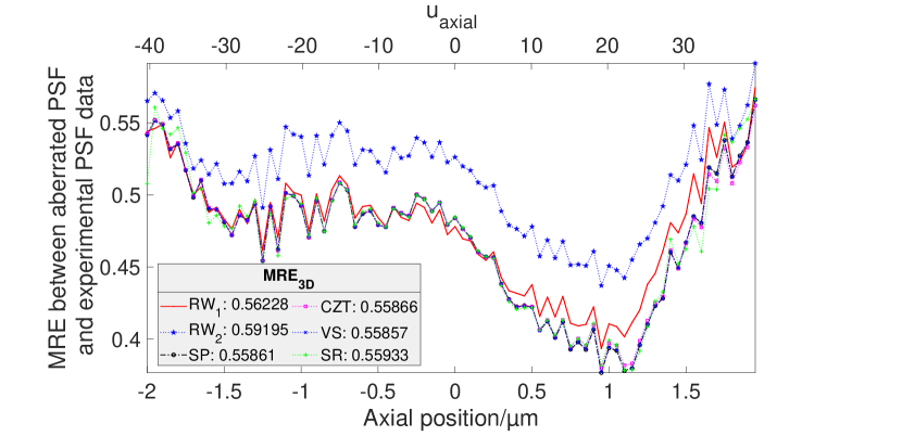
(b)

Figure 20: Evaluation of the similarity and difference between the experimental PSF data and the theoretical PSFs which are aberrant by the retrieved phase from the experimental data. (a) Similarity quantified by the NCC. (b) Difference quantified by the MRE.

V.2.4 Second set of comparison: non-aberrant PSFs

The errors considered in the first set of comparison include error due to phase retrieval. To not consider that error and to include the state-of-art PSFs into the comparison, we compare non-aberrant theoretical PSFs with the experimental data in a region of interest where the aberration and noise in the experimental data are minimal. Firstly, to check the region where aberrations are minimal, we conduct a slice by slice comparison between the computed theoretical aberrant PSF described in Section V.2.3 and the corresponding non-aberrant PSFs. The NCC results are displayed in Fig. 21. Secondly, as we would want to compare our non-aberrant models with an experimental data having as little noise as possible, the standard deviation (Std) of the experimental data is calculated at each axial position (see Fig. 21). We fit this Std distribution into a Gaussian function. The Std distribution is not originally centered to $z=0$ so we shift it to zero accordingly. The same shift in $z$ is applied to the experimental measured PSF data before the region of interest is extracted. To construct a comparison metric, we thus chose a common region where the slicewise NCC (after z-alignment) is high. This corresponds to positions near the focus where the Std is above half of its maximum as estimated by a Gaussian fit (Fig. 21). This region of interest is indicated by the red dashed rectangle in Fig. 18(a).

The NCC results between the experimental data and the non-aberrant theoretical data within the region of interest are displayed in Fig. 22.

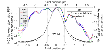
Figure 21: Selection of the region of interest (ROI) for comparing the non-aberrant PSFs with experimental PSF data. The ROI is the volume delimited by the full-width half maximum (FWHM) of the Gaussian fit of the standard deviation (Std) of the experimental data along the axial axis. The Std distribution is normalized by its maximum for display.

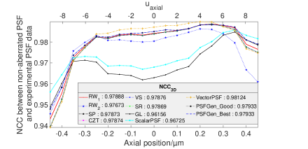
Figure 22: NCC between experimental PSF and non-aberrant theoretical PSFs within a particular region of interest near the focus.

V.2.5 Discussion

By observing Fig. 20, on one side we can conclude that there is a high similarity between the aberrant theoretical PSFs with the experimental data. On the other side, the MRE results are not symmetric about the focus. This asymmetry is explained by the fact that the shift of focus in the experimental measured PSF was not perfectly retrieved through the phase retrieval technique. This induces the error detected in the MRE since the computation of the MRE is conducted point by point and slice by slice. However, we can conclude from the graph that SP, CZT and VS are the models which have higher similarity and less error compared to the experimental data.

By considering the region of interest where the signal-to-noise ratio is higher and the aberration is small, the quantification of the NCC between the non-aberrant PSFs and the experimental data allows us to short the models in order of accuracy. The VectorPSF described in reference Aguet et al. (2009) leads with a $3$D NCC equal to $0.98124$. This lead is followed closely by PSFGen_Good and PSFGen_Best in reference Kirshner et al. (2013), RW₁, VS, CZT, SP, SR, ScalarPSF Aguet et al. (2009), RW₂ and GL in reference Li, XUE, and BLU (2017). The scalar PSFs are the least accurate especially near the focus in this particular comparison. The difference in NCC between the models and with the experimental data is however very close for the vector PSF models.

VI Conclusion

In this work, we provided a general approach for calculating the $3$D PSF of a system satisfying the Abbe sine condition. We focused on Fourier based techniques and compared the results of a variety of PSF calculations schemes with a gold standard from a Richard and Wolf model computed at higher sampling. We explained the algorithmic details of each technique and potential advantages and pitfalls. The Fourier models agree with high precision with the state-of-the-art and are validated experimentally to have good accuracy around the focus. We also showed in this work that vector PSFs are more accurate than scalar models. The study of the PSFs at higher depth of focus as well as the inclusion of refractive index mismatching in the theoretical model is not covered in this work. This constitutes the next step for PSFs comparisons in addition to the test of each model in image reconstruction (deconvolution). The Fourier based $3$-D PSF models are already fast enough given the fact that there is no radial symmetry included in them. The models discussed in this manuscript are under the condition that all the planes in the optical system are perpendicular to the optical axis. The ability of our models to accommodate radial asymmetry is advantageous compared to the state-of-the-art because our models can accommodate any non-circular aberration and tilted planes caused in the system such as a tilt of a coverslip. We plan to combine some of the models such that the computation is still faster without compromising the accuracy of the models at any axial depth $z$. The models can be adjusted for confocal microscopy, STED (Stimulated emission depletion microscopy) and PSF engineering.

Funding

This work was funded by the DAAD through the African Institute for Mathematical Sciences and Stellenbosch University, and Friedrich Schiller University Jena. This work was also supported by the German Research Foundation (DFG) through the Collaborative Research Center PolyTarget 1278, project number 316213987, subproject C04 and the Council for Scientific and Industrial Research (CSIR), project number LREQA03.