A High Precision Survey of the D/H Ratio in the Nearby Interstellar Medium

Abstract

We present high S/N measurements of the H I Ly$\alpha$ absorption line toward 16 Galactic targets which are at distances between approximately 190 and 2200 pc, all beyond the wall of the Local Bubble. We describe the models used to remove stellar emission and absorption features and the methods used to account for all known sources of error in order to compute high precision values of the H I column density with robust determinations of uncertainties. When combined with H₂ column densities from other sources, we find total H column densities ranging from 10^20.01 to 10^21.25 cm${}^{-2}.$ Using deuterium column densities from FUSE observations we determine the D/H ratio along the sight lines. We confirm and strengthen the conclusion that D/H is spatially variable over these H I column density and target distance regimes, which predominantly probe the ISM outside the Local Bubble. We discuss how these results affect models of Galactic chemical evolution. We also present an analysis of metal lines along the five sight lines for which we have high resolution spectra and, along with results reported in the literature, discuss the corresponding column densities in the context of a generalized depletion analysis. We find that D/H is only weakly correlated with metal depletion and conclude that the spatial D/H variability is not solely due to dust depletion. A bifurcation of D/H_tot as a function of depletion at high depletion levels provides modest support that deuterium-rich gas is infalling onto the Galactic plane.

1. Introduction

The observed abundance of deuterium is one of the cornerstones of modern cosmology. Building on the idea that some elements more massive than hydrogen could be synthesized in the first few minutes of the Big Bang (e.g., von Weizsäcker, 1938; Gamow, 1948) combined with the discovery of the cosmic microwave background, detailed predictions of the abundances of deuterium and helium from Big-Bang nucleosynthesis (BBN) were developed in the 1960s (Peebles, 1966; Wagoner et al., 1967). Subsequently, measurements of deuterium in the diffuse interstellar medium (ISM) of the Milky Way (Rogerson & York, 1973; York & Rogerson, 1976) were found to be in good agreement with the predictions of BBN, which provided a spectacular confirmation of Big Bang theory and an estimate of the baryonic content of the universe.

The utility of deuterium abundances in the ISM as a probe of the early universe depends on the importance of subsequent processes that can either destroy or produce this isotope as the Galaxy evolves. On the one hand, we know for certain that deuterium is destroyed in stars (astration). The importance of this effect depends on how much of the stellar material replenishes the gas in the ISM and how much this loss of deuterium is balanced by contributions that comes from the infall of pristine gas from the intergalactic medium. A general consensus from modeling these processes in our Galaxy is that D/H probably does not decrease from the primordial value by more than a factor of about 2 (Steigman & Tosi, 1992; Vangioni-Flam et al., 1994; Galli et al., 1995; Steigman & Tosi, 1995; Dearborn et al., 1996; Prantzos, 1996; Chiappini et al., 2002; Romano et al., 2006; Prodanović & Fields, 2008; Leitner & Kravtsov, 2011; Weinberg, 2017).

On the other hand, we also must be aware of processes after BBN that can create new deuterium.This was first investigated by Epstein, Lattimer, & Schramm (1976) who considered both synthesis and spallation production mechanisms including pregalactic cosmic rays, shock waves, hot explosions, and the disruption of neutron stars by black holes. They concluded that post Big-Bang deuterium production requires extremely violent and exotic conditions for which there is little supporting evidence and most processes would over- or under-produce other light elements, which other observations have adequately constrained. However, Mullan & Linsky (1998) pointed out that these investigators neglected a potentially important process, the production of neutrons in stellar flares which are then captured by protons to form D, and this could be an important source of interstellar deuterium. Prodanović & Fields (2003) subsequently examined this hypothesis in more detail and ruled out this mechanism as a significant source of D on the Galactic scale based on observed limits of the 2.22 MeV $\gamma$-ray produced by this reaction. However, they do agree that this process must occur at some level and the possibilty of very local enrichment, while not likely, cannot be ruled out entirely. A more exotic creation process is the proposal by Gnedin & Ostriker (1992) that deuterium could be produced by the photodisintgration of ⁴He by gamma rays produced by the accretion of gas onto $10^{6}\,{\rm M}_{\odot}$ black holes. Although a black hole with a mass comparable to this exists at the center of the Milky Way, it has not been shown that it has produced an appreciable amount of deuterium in the region of the Galaxy that is the subject of our investigation, and in any case this probably would not cause abundance variations over the scales we are probing. Lubowich, et al. (2000) measured the distribution of DCN relative to HCN in a molecular cloud only 10 pc from the Galactic center and conclude that D/H = $1.7\pm 0.3$ ppm (parts per million), far below any region in the local ISM. Lubowich & Pasachoff (2010) measured this ratio in 16 molecular clouds at galactocentric distances ranging from 2 pc to 10 kpc. They find that D/H increases slightly with distance to a maximum of 20.5 ppm. Both studies conclude that the observed deuterium is cosmological and there are no other significant sources. In this study we therefore assume, as most studies have since Epstein, Lattimer, & Schramm (1976), that all observed deuterium is primordial in origin. Consequently, the observed deuterium abundance may provide an unambiguous probe of the chemical evolution of gas in galaxies (i.e., the processing of gas due to cycling through stars).

However, as more interstellar D/H detections have accumulated, the interpretation of the deuterium abundances has become less clear. The ensemble of D/H measurements from the Copernicus and International Ultraviolet Explorer (IUE) satellites seemed to indicate that D/H is spatially variable in the Milky Way, which caused some tension between BBN and galactic evolution models (Laurent et al., 1979; Vidal-Madjar & Gry, 1984; Vidal-Madjar et al., 1998; Hébrard et al., 1999). The reality of the variability was challenged based on uncertainties of the early measurements (McCullough, 1992), but subsequent (and more precise) D/H determinations with the ORFEUS-SPAS II Interstellar Medium Absorption Profile Spectrograph (IMAPS) and with the Far Ultraviolet Spectroscopic Explorer (FUSE) have continued to provide compelling evidence that D/H varies from place to place in our Galaxy (Jenkins et al., 1999; Sonneborn et al., 2000; Moos et al., 2002; Wood et al., 2004; Linsky et al., 2006) (hereafter L06).

Today, deuterium measurements in the lowest metallicity, high-redshift QSO absorption systems are preferred for cosmological purposes in order to measure a D/H abundance that is close to the primordial value and minimally confused by astration (e.g., O’Meara et al., 2006; Pettini & Cooke, 2012; Cooke et al., 2018; Zavarygin et al., 2018). The metallicity of the Milky Way ISM is 5-600 times higher than the metallicity of the QSO absorbers typically used to constrain the primordial D/H and cosmological baryon density (Cooke et al., 2018), but the Milky Way measurements are still relevant for two reasons. First, it is important to understand the origin of the spatial variability of D/H in the Galactic ISM in order to ensure that the high-redshift measurements are also interpreted correctly. After years of work high$-z$ D/H measurements have now fairly well converged but do exhibit some scatter (see, e.g., Figure 7 in Cooke et al., 2018). We want to understand this deuterium variability to make sure we are interpreting all of these results correctly. The Milky Way ISM is likely the best laboratory for probing the physical processes that affect D/H. Second, by comparison with high-redshift measurements, Milky Way deuterium abundances constrain models of the chemical evolution of our Galaxy.

One possible explanation for the Galactic D/H variability is that the Milky Way could still be accreting relatively pristine gas with a high deuterium abundance and a low metallicity. The Galactic high-velocity cloud Complex C is an example of a sub-solar metallicity cloud with a high deuterium abundance that appears to be falling into the Milky Way (Sembach et al., 2004); if infalling clouds like Complex C have merged into the Galactic ISM but are poorly mixed, this could lead to patchy (spatially variable) deuterium abundances. However, in this scenario an anticorrelation between metallicity and D/H would be expected because the processing inside stars that destroys D also creates metals. This anticorrelation does not appear to be present in the data (Hébrard & Moos, 2003) but it is important to confirm this result with larger samples and precise measurements.

Table 1Stellar Information and STIS Observation Log

Object	$l$	$b$	$V$	Obs Date	Exp. Time	Grating ($\lambda_{c}$)	Aperture	Dataset
	($\deg$)	($\deg$)	(mag)		(s)	(Å)	(arcsec)
HD 191877	61.6	$-6.45$	6.26	2011-06-17	1183	E140H (1271)	0.1x0.03	OBIE08010
BD+39 3226	65.0	28.8	10.2	2011-07-24	1757	E140H (1271)	0.2x0.09	OBIE09010
Feige 110	74.1	$-59.1$	11.4	2010-12-12	1734	G140M (1218)	52x0.05	OBIE01010
PG 0038+199	119.8	$-42.7$	14.5	2010-12-31	1882	G140M (1218)	52x0.05	OBIE10010
HD 41161	165.0	12.9	6.76	2010-12-12	1433	E140H (1271)	0.1x0.03	OBIE11010
HD 53975	225.7	$-2.3$	6.48	2011-10-02	1161	E140H (1271)	0.1x0.03	OBIE12010
TD1 32709	233.0	28.1	12	2011-05-06	1732	G140M (1218)	52x0.05	OBIE13010
WD 1034+001	247.6	47.8	13.2	2011-04-20	1904	G140M (1218)	52x0.05	OBIE14010
LB 3241	273.7	$-62.5$	12.7	2011-06-24	2070	G140M (1218)	52x0.05	OBIE07010
LSS 1274	277.0	-5.3	12.9	2011-04-14	0	G140M (1218)	52x0.05	…
HD 90087	285.2	$-2.1$	7.8	2011-09-27	2038	E140H (1271)	0.2x0.09	OBIE15010
CPD$-$71 172	290.2	$-42.6$	10.7	2011-08-21	1847	G140M (1218)	52x0.05	OBIE05010
LB 1566	306.4	$-62.0$	13.1	2011-07-09	2185	G140M (1218)	52x0.05	OBIE06010
LSE 44	313.4	13.5	12.5	2011-07-12	2071	G140M (1218)	52x0.05	OBIE04010
JL 9	322.6	$-27.0$	13.2	2011-07-22	2301	G140M (1218)	52x0.05	OBIE16010
LSE 234	329.4	$-20.5$	12.6	2011-02-06	2197	G140M (1218)	52x0.05	OBIE17010
LSE 263	345.2	$-22.5$	11.3	2011-05-26	1479	G140M (1218)	52x0.05	OBIE03010

A second hypothesis, originally proposed by Jura (1982), is that the D/H spatial variability is due to depletion by dust grains, which might more effectively remove D than H (Tielens, 1983; Draine, 2004, 2006). In this case, a correlation between D/H and abundances of depletable metals would be expected: increased dust content would lead to a lower D/H ratio in the gas phase (a higher portion of the D would be stuck on dust grains) as well as lower gas-phase abundances of metals that tend to be incorporated into dust (e.g., titanium, nickel, or iron). The first observational support for this hypothesis was provided by Prochaska et al. (2005), who found that D/H and Ti/H are correlated at 95% confidence. Further evidence supporting this explanation was subsequently reported by L06, Ellison et al. (2007), and Lallement et al. (2008). Some other aspects of the observations do not entirely fit with the dust-depletion hypothesis. For example, sight lines with low H₂ fractions and low values of the $E_{B-V}$ color excess would be expected to have high D/H values because little depletion should occur, but the opposite is observed – some sight lines with low $E_{B-V}$ and low H₂ fractions also have low D/H ratios. Likewise, some of the directions with high H₂ fractions have the highest D/H ratios (Steigman et al., 2007). These unexpected behaviors implicitly assume that all species (D, metals, molecules, and dust) share similar distribution with similar fractional abundances regardless of the sight line considered, which is not necessarily true (Welty et al., 2020) and is difficult to verify with the data at hand. When combined with the presence of significant outliers and the peculiar slopes in the relationships between D/H and depleted metal abundances (Ellison et al. 2007), this potential degeneracy also makes the dust-depletion hypothesis more problematic to probe.

This paper is organized as follows. In Section 2 we describe some practical considerations in the choice of observing strategy for this program and in Section 3 we describe the targets and observing details. In Section 4 we discuss the computation of the stellar models used in the modeling of the interstellar Ly$\alpha$ absorption line. In Section 5 we describe in detail the computation of the H I column density and its associated error. Our objective is to determine D/H and we rely on published values of $N$(D i). However, there are no published values of this for five of our targets, and in Section 6 we discuss our measurements of $N$(D i) for these targets. In Section 7 we describe the principal results of this study, our new D/H results along 16 lines of sight, and how they compare with previous measurements in the high $N$(H i) regime. In Section 8 we describe our abundance measurements of various metals in the five targets for which we obtained high resolution spectra. The correlation of these abundances with D/H and their interpretation in terms of a unified depletion analysis is given in Section 9. In Section 10 we discuss our results in the broader context of the distribution of D/H measurements as a function of $N$(H i), the evidence for depletion of deuterium onto dust grains and for infall of deuterium rich material, and how our results fit into models of Galactic chemical evolution. We summarize the results of this study in Section 11.

2. Practical Considerations

Ironically, in many interstellar sight lines, the column density of the much rarer deuterium isotope is easier to measure than the column density of the abundant H i, and in many cases the uncertainty in D/H is dominated by the uncertainty in $N$(H i) (L06). When the H i column is high enough so that D i can be detected, most of the higher H i Lyman series lines are strongly saturated but do not exhibit well-developed damping wings; the H i Ly$\alpha$ line must be observed to tightly constrain $N$(H i). Consequently, many FUSE observations (which do not cover Ly$\alpha$) provide precise measurements of $N$(D i) but only very crude constraints on $N$(H i). In some cases, FUSE results can be combined with Hubble Space Telescope (HST) spectra of Ly$\alpha$ resulting in exquisite D/H measurements (e.g., Sonneborn et al., 2002). Unfortunately, for some of the key sight lines, only single, low-quality IUE spectra of the H i Ly$\alpha$ line were available for the analyses above (if any Ly$\alpha$ data were available at all), and the uncertainties in $N$(H i) were large and dominated by difficult to assess systematic errors (Friedman et al., 2002, 2006). For example, the significance of the correlation between D/H and Ti/H observed by Prochaska et al. (2005) hinges on the sight line to Feige 110, which unfortunately has a very uncertain H i column derived from a single, poor-quality IUE spectrum (Friedman et al., 2002). Likewise, outliers in the various studies above could be spurious measurements due to poor $N$(H i) constraints, or they could be real outliers that indicate that the spatial variability is not necessarily due entirely to dust depletion. Better measurements are needed to understand the D/H variability and its implications.

To rectify the uncertainties in D/H measurements due to poor or non-existent H i Ly$\alpha$ data, we embarked on a program in HST Cycle 18 to obtain much better H i Ly$\alpha$ spectra using the Space Telescope Imaging Spectrograph (STIS) (Kimble et al., 1998; Woodgate et al., 1998) on HST. This spectrograph provides vastly better spectra of the Ly$\alpha$ line (see, e.g., Figure 4 in Sonneborn et al., 2002) than IUE and enables precise measurement of $N$(H i) even in cases where the interstellar Ly$\alpha$ is blanketed with narrow stellar lines (Sonneborn et al., 2002). Moreover, the new STIS spectra have high spectral resolution and enable measurement of a variety of metal column densities including species such as O i, Mg ii, P ii, Cl i, Mn ii, Ni ii, and Ge ii, so the new STIS data also enable improvements of the metal measurements. In this paper we present the findings of this study.

Table 2Stellar Parameters Used for the Model Atmospheres

Star	Sp Type	$T_{\rm{eff}}$	$\log g$	$\log N({\rm{He}})/N({\rm{H}})$	$v\sin i$	$Distance\tablenotemark{a}$	Ref.
		(K)	(cm s-2)		(km s-1)	(pc)
Hot Subdwarfs
BD+39 3226	He-sdO	$45970\pm 1000$	$6.05\pm 0.10$	$0.50\pm 0.10$	$\cdots$	$189\pm 2$	1
Feige 110	sdOB	$44745\pm 2000$	$5.96\pm 0.15$	$-1.78\pm 0.10$	$\cdots$	$271\pm 4$	2
TD1 32709	He-sdO	$46500\pm 1000$	$5.60\pm 0.15$	$2.0\pm 0.3$	$31\pm 3$	$522\pm 16$	3,4,5
LB 3241	sdO	$42200\pm 2000$	$5.60\pm 0.20$	$<-3.3$	$\cdots$	$653\pm 18$	2
CPD$-$71 172	sdO	$60000\pm 5000$	$5.4\pm 0.2$	$-1.0$	$\cdots$	$328\pm 2$	6
LB 1566	He-sdO	$49320\pm 2000$	$5.84\pm 0.20$	$>1.8$	$\cdots$	$823\pm 26$	2
LSE 44	sdO	$39820\pm 2000$	$5.50\pm 0.20$	$-2.90\pm 0.10$	$\cdots$	$615\pm 15$	2
JL 9	He-sdO	$75000\pm 5000$	$5.50\pm 0.25$	$0.21\pm 0.10$	$\cdots$	$1592\pm 78$	2
LSE 234	sdO	$90000\pm 5000$	$6.0\pm 0.3$	$-1.0\pm 0.1$	$\cdots$	$601\pm 16$	7
LSE 263	He-sdO	$70000\pm 2500$	$4.90\pm 0.25$	$>1.0$	$\cdots$	$719\pm 59$	8
White Dwarfs
PG 0038+199	DO	$125000\pm 5000$	$7.0\pm 0.5$	$1.7$	$\cdots$	$400\pm 7$	9
WD 1034+001	DO	$115000\pm 5000$	$7.0\pm 0.5$	$>1.9$	$\cdots$	$193\pm 2$	9
O and B Stars
HD 191877	B1.0 Ib	21700	2.67	$\cdots$	152	$1811\pm 141$	10,11,12
HD 41161	O8.0 Vn	34877	3.92	$\cdots$	296	$1489\pm 134$	13,14,15
HD 53975	O7.5 Vz	35874	3.92	$\cdots$	163	$1154\pm 65$	13,14,12
HD 90087	O9.0 II	31607	3.38	$\cdots$	259	$2193\pm 126$	16,14,15

References. — (1) Chayer, Green, & Fontaine (2014); (2) This study; (3) Dreizler (1993); (4) Schindewolf et al. (2018); (5) Hirsch (2009); (6) Deleuil & Viton (1992); (7) Haas et al. (1995); (8) Husfeld et al. (1989); (9) Werner et al. (2017); (10) Lesh (1968); (11) Searle et al. (2008); (12) Howarth et al. (1997); (13) Sota et al. (2011); (14) Martins, Schaerer, & Hillier (2005); (15) Penny (1996); (16) Garrison, Hiltner, & Schild (1977).

3. Target Selection and Observations

The Local Bubble (LB) is a volume of space that contains a mixture of low density ionized and neutral gas in which the Sun is embedded (Breitschwerdt, 1998) and has an irregular boundary about $100-300$ pc from the Sun (Pelgrims, 2020). This boundary consists of neutral hydrogen, so sight lines with $N$(H i) $\gtrsim 10^{19.2}$ cm^-2 usually extend beyond the LB into the more distant ISM. Previous work has shown that D/H is approximately constant within the LB but it exhibits considerable variability beyond it (see Figure 1 in L06). To investigate the cause of this variability we selected targets that (1) lie outside the LB, (2) have FUSE spectra of sufficient quality to permit accurate computation of $N$(D i) or that such published values already exist, and (3) that the stellar fluxes were appropriate to obtain excellent Ly$\alpha$ profiles in a single HST orbit. The 17 targets selected as part of program ID 12287 are listed in Table 1 along with various exposure parameters. Sixteen targets were successfully observed.

The targets of choice for studying sight lines just beyond the LB are hot subdwarf stars (spectal type sdB, sdOB, sdO, He-sdO). Hot stars are favored because their flux peaks in the ultraviolet where several interesting atomic transitions occur, and subluminous stars because their spatial density allows the observation of bright stars at distances of a hundred to several hundred parsecs. To the distances where we find these hot subdwarfs, we can add the extremely hot white dwarfs, although they are much less numerous than the hot subdwarfs. At distances well beyond the LB, O and B stars are used to explore long sight lines. Although these faint and bright blue stars are suitable targets for studying the interstellar H I Ly$\alpha$ line, their stellar spectra present challenges for measuring accurate H I column densities.

The spectra of 11 targets were obtained using the first order grating G140M on STIS. This setup provides a very clean spectrum spanning approximately $1192-1245$ Å at a velocity resolution of $\sim 30$ km s^-1, which is adequate for measuring $N$(H i) using the damping wings of the Ly$\alpha$ line. Five targets were too bright to be observed with G140M and were instead observed in echelle mode with the E140H grating, spanning $1164-1356$ Å at a resolution of $\sim 2.6$ km s^-1, which is sufficient for measuring metal abundances for these sight lines, as discussed in Section 8. A potential disadvantage of this observing configuration is that echelle reductions can suffer from imperfect ripple corrections, causing the spectral orders to be improperly joined. We found that the IDL procedure hrs_merge.pro produced excellent 1-d spectra and no further correction was required. The standard pipeline-reduced data show zero flux at the center of the saturated Ly$\alpha$ cores (aside from minor geocoronal Ly$\alpha$ emission) so no additional background correction was required for any spectrum. We note that the flux zero point was an especially troublesome issue for many previous analyses, especially those that relied on IUE observations (see e.g., Friedman et al. (2006)).

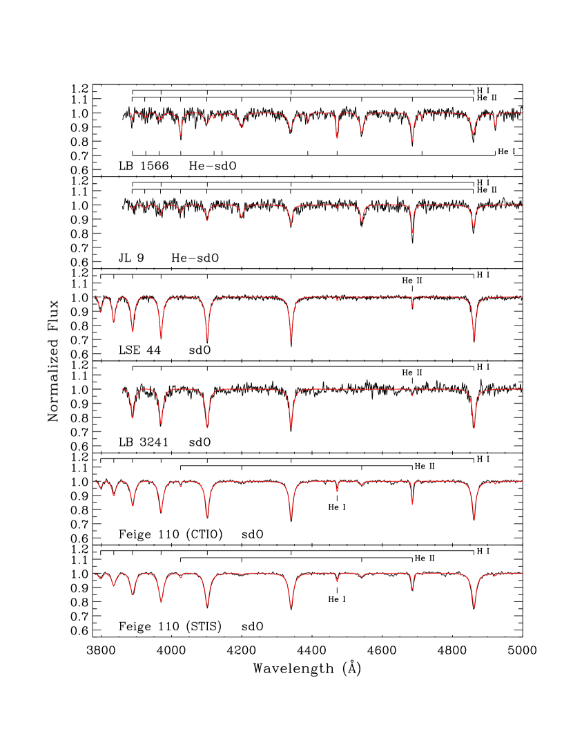
Figure 1.— Best model-atmosphere fits to the optical spectra of the hot subdwarf stars analyzed in this study. The names of the stars with their spectral types are given in each panel along with identifications of H I, He I, and He II lines. Two optical spectra are available for Feige 110 and both are used to estimate the uncertainties of the atmospheric parameters.

4. Stellar Models

In order to take into consideration the stellar contributions to the Ly$\alpha$ line profile and the placement of the continuum, we computed synthetic spectra using stellar atmosphere models. We used the stellar atmosphere and spectrum synthesis codes TLUSTY (Hubeny & Lanz, 1995) and Synspec to compute non-local thermodynamic equilibrium (NLTE) stellar atmosphere models and synthetic spectra. Both codes were developed by I. Hubeny and T. Lanz. A detailed description and use of the codes are presented in a series of three papers by Hubeny & Lanz (2017a, b, c). Synthetic spectra are calculated from models of stellar atmospheres that describe the surface properties of stars and are based on the results of spectroscopic data analysis. Table 2 gives the atmospheric parameters of the 16 stars considered in this study. These parameters are the surface gravity, the effective temperature, and the number ratio of helium-to-hydrogen. We also take into account the chemical composition of the atmospheres which is important for hot stars and in particular hot subdwarfs and white dwarfs. These high-gravity stars show abundance anomalies that arise from the effects of diffusion. We determined the atmospheric parameters of five stars in this study, and collected the parameters of other stars from the literature.

The atmospheric parameters of these five stars were determined by fitting the H and He lines observed in optical spectra with two grids of NLTE atmosphere models. LB 3241, LB 1566 and JL9 were observed with the CTIO 1.5-m Cassegrain spectrograph by H.E. Bond in 2011. The spectrograph was configured to use the 26/Ia grating and a slit of 110 $\mu$m. This configuration produced wavelength coverage ranging from 3650 to 5425 Å and spectral resolution of FWHM = 4.3 Å. JL 9 and LB 1566 have exposure times of 400 s each while LB 3241 has an exposure time of 350 s. The signal-to-noise ratio from each exposure is about 50. The optical spectra of Feige 110 and LSE 44 are described in Friedman et al. (2002, 2006). As Feige 110, LB 3241, and LSE 44 are He-poor stars, we used the grid of NLTE models for extreme horizontal branch stars developed by Brassard et al. (2010). This grid covers the ranges of 20,$000\leq T_{\rm{eff}}\leq 50$,000 K in steps of 2000 K, $4.6\leq\log g\leq 6.4$ in steps of 0.2 dex, and $-4.0\leq\log(N(\rm{He})/N(\rm{H}))\leq 0.0$ in steps of 0.5 dex. These models assume a metallicity of C = 0.1, N = 1.0, O = 0.1, S = 1.0, Si = 0.2, and Fe = 1.0 $\times$ solar values (Grevesse & Sauval, 1998), which is typical of these H-rich stars. For the He-rich stars LB 1566 and JL 9, we used our own grid of NLTE H-He models that covers the ranges 30,$000\leq T_{\rm{eff}}\leq 98$,000 K in steps of 2000 K, $4.8\leq\log g\leq 7.0$ in steps of 0.2 dex, and $0.0\leq\log(N(\rm{He})/N(\rm{H}))\leq 3.0$ in steps of 0.5 dex. Figure 1 shows our best fits to the optical spectra. The effective temperature of JL 9 was increased from 68,820 K obtained from the optical fit alone to 75,000 K, as shown in Table 2, in order to reproduce the ionization balance of the Fe VI and Fe VII ions which are observed in the FUSE and STIS spectra. Werner et al. (2022) came to a similar conclusion although their temperature and gravity are somewhat different with $T_{\rm{eff}}=80,000\pm 5000$ K and $\log g=5.2\pm 0.3,$ but the error analysis described in Section 5.1 shows that this has a negligible effect on the value of $N$(H i) we obtain.

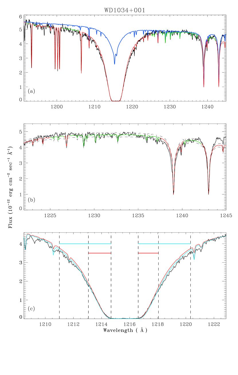
Figure 2.— The spectrum of WD1034+001 in detail. (a) The observed spectrum is shown in black and our best fit model spectrum in red. The spectral regions that are used to constrain the polynomial fit to the continuum are shown in green. The blue line is the model of the stellar atmosphere. (b) An expanded view of the long-wavelength portion of the spectrum showing a continuum region and the stellar absorption lines used to constrain the radial velocity of the stellar model. The dashed lines show the high and low continuum scalings used to determine the contribution of continuum placement errors to the error in $N$(H i). (c) An expanded view of the Ly$\alpha$ line. $N$(H i) and the radial velocity of the interstellar H I are most strongly constrained in the spectral regions just outside the black core of the absorption line. The nominal spectral region used to constrain these parameters is shown by the red horizontal bars and corresponds to the red spectrum. To estimate the error associated with the choice of spectral region, we also calculate $N$(H i) and the radial velocity based on the extended region indicated by the cyan horizontal bars and the corresponding cyan spectrum. The spectral coverage indicated by the red and cyan bars differs for each target. See text for a discussion of the extent of these bars and of the discrepancy between the black and red spectra in the upper wings of the damped Ly$\alpha$ profile.

As Table 2 indicates, we placed our targets into three classes: Hot subdwarfs, white dwarfs, and O and B stars. For each star, we calculated stellar atmosphere models which are based on the atmospheric parameters and their uncertainties, and the abundances of metals published in the literature (see references in Table 2). For those stars that did not have metal abundances, we used FUSE and STIS spectra to determine their abundances. In the case of O and B stars, we used the grids of model atmospheres that were calculated by Lanz & Hubeny (2003, 2007). In order to take into account the effect of atmospheric parameter uncertainties on the stellar contribution to the determination of H I column densities, we calculated models at the extremes of effective temperature and gravity. Models with $T_{\rm{eff}}-\Delta T_{\rm{eff}}$ and $\log g+\Delta\log g$ produce stronger Ly$\alpha$ and $\lambda$1215 He II stellar lines, while models with $T_{\rm{eff}}+\Delta T_{\rm{eff}}$ and $\log g-\Delta\log g$ produce weaker lines (see Section 5.1). Synthetic spectra were calculated from these atmosphere models. They have been calculated to cover the wavelength ranges of the low and high resolution STIS spectra. They were convolved with Gaussians of FWHM = 0.1 and 0.03 Å, respectively. Finally, a rotational convolution was performed on the spectra for stars with high $v\sin i$ values. In some cases the models were better constrained than previous ones in the literature due to accurate distances provided by the Gaia DR3 (Soszyński, 2016; Vallenari et al., 2022).

5. Measurement of $N$(H i)

In this section we describe the method used to compute the interstellar H I column density. There are 9 adjustable parameters in our fits to the observed spectra. They are the coefficients of the 6th order polynomial fit in clear portions of the continuum region adjacent to the Ly$\alpha$ absorption line; the radial velocity of the modeled stellar spectrum with respect to the observed spectrum; the radial velocity of the modeled interstellar Ly$\alpha$ absorption with respect to the observed spectrum; and, of course, the value of $N$(H i) itself. The b-value of the absorbing gas is not important because the Gaussian part of the Voigt profile is buried deep inside the black core of the strong Ly$\alpha$ line.

Figure 2 illustrates how we measure the H I column density by examining the spectrum of WD1034+001 in detail. The first step is to select regions of the continuum which are relatively free of absorption lines, over which the polynomial will be fit. These are shown in green in panel (a). Note that we have used continuum regions on both the blue and red sides of Ly$\alpha$. (For HD90087 there is so much absorption on the blue side of Ly$\alpha$ that the continuum never recovers, so only the red side was used to constrain the polynomial.) The purpose of this polynomial fit is to remove residual instrumental variations and the wavelength dependent reddening by dust. Next, the radial velocity of the stellar model is adjusted based on selected stellar absorption lines, such as those shown in the expended red spectral region in panel (b). We avoided lines that might have a significant interstellar contribution. For WD1034+001 we used the strong N V $\lambda\lambda 1238,1242$ doublet. The remaining weak stellar lines do not significantly improve the constraint on the radial velocity in this case, but they match the model well. We then fix the stellar velocity so the automated fitting program does not try to assign the stellar lines to one of the many interstellar features in the spectrum. The final value of $N$(H i) is insensitive to this velocity since the stellar H I and He II absorptions (the most prominent absorption lines in the stellar model, shown in blue in panel (a)) are almost completely contained within the black core of the interstellar H I absorption.

Next we do a simultaneous fit of the remaining 8 parameters listed in the previous paragraph by minimizing $\chi^{2}$ between the model and observed spectra in the green continuum regions shown in panel (a) and in the damping wings of the Ly$\alpha$ profile as shown in panel (c). For this task we used the amoeba software routine in IDL. In the $\chi^{2}$ calculation that minimizes the outcome for $N$(H i) we assigned greater weight to the Ly$\alpha$ region than to the continuum regions because we did not want difficulties in the continuum fit to compromise the important Ly$\alpha$ fit, particularly in continuum regions far from the Ly$\alpha$ line which are unimportant for the determination of the H I column density.

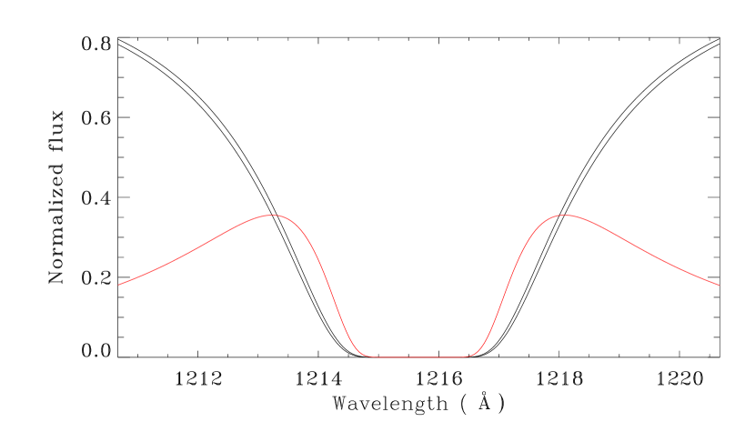
Figure 3.— The top black curve shows the continuum-normalized Ly$\alpha$ profile with no other interstellar or stellar absorption lines for log($N$(H i)) = 20.12, corresponding to the column density of WD1034+001. The bottom black curve is for log($N$(H i)) greater by 0.03 dex. The red curve is the difference between these profiles multiplied by 15 to more clearly show the wavelengths where the two damped profiles differ the most. The peak of this curve guided our selection of the Ly$\alpha$ fitting region described in Section 5.1. Note that our total error on the logarithmic H I column density for every sight line in this study is between 0.01 and 0.02 dex, which is considerably less than the difference displayed in this illustration.

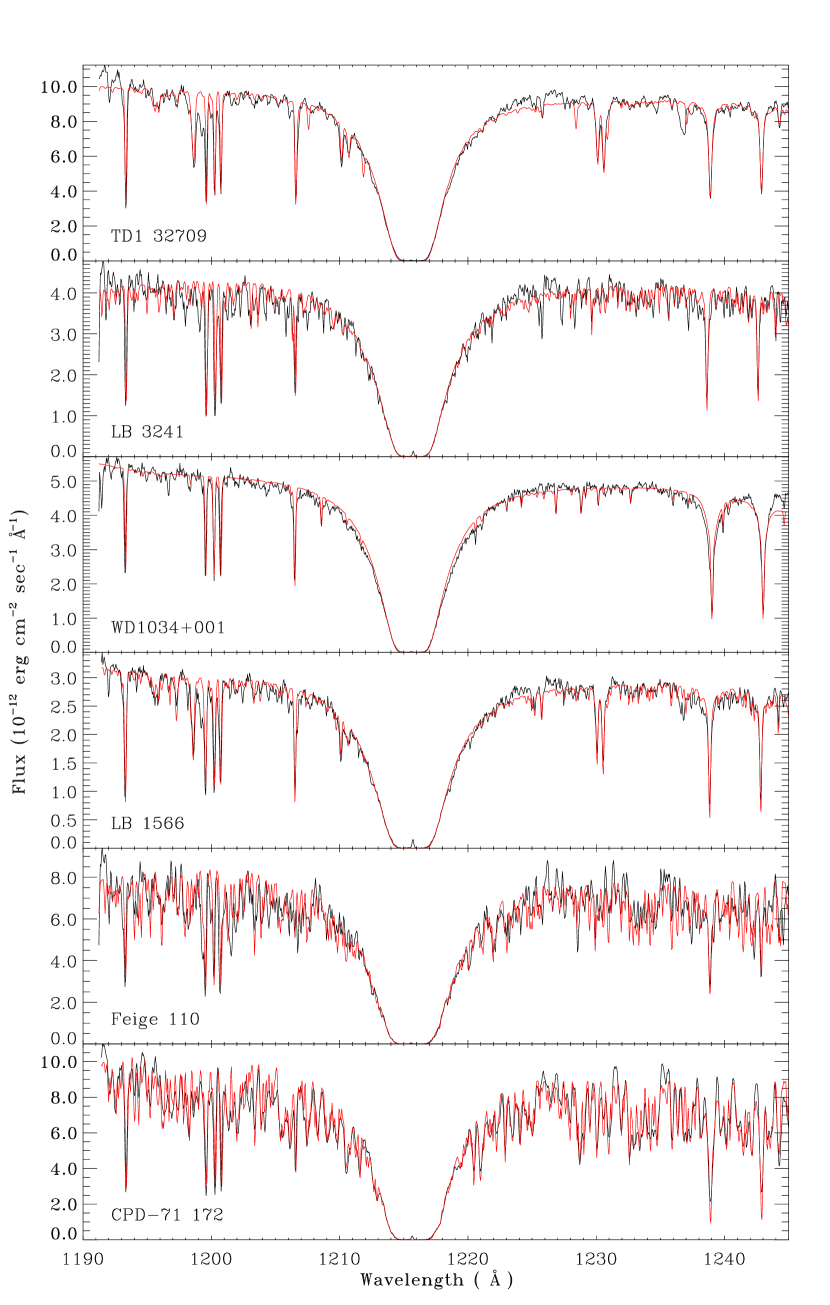
Figure 4.— Observed STIS spectra (in black) obtained with the STIS medium resolution G140M grating, plotted with our model spectra (in red). The objects are labelled in each panel and are shown in order from lowest (top) to highest (bottom) values of $N$(H i). The small peak in the core of the Ly$\alpha$ line in some spectra is due to geocoronal Ly$\alpha$ emission.

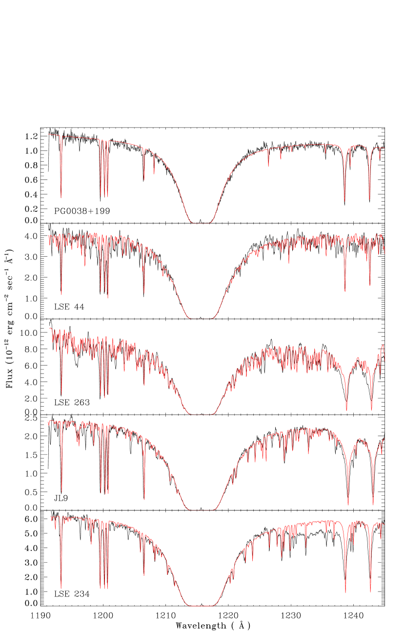
Figure 4.— (Continued)

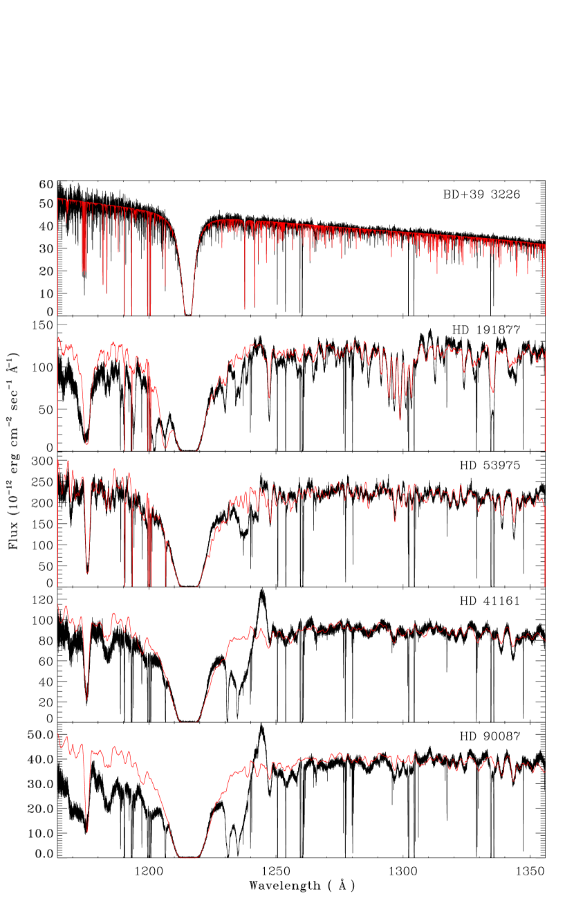
Figure 5.— Observed STIS spectra (in black) obtained with the STIS high resolution E140H echelle grating, plotted with our model spectra (in red). The objects are shown in order from lowest (top) to highest (bottom) values of $N$(H i).

We now consider the proper spectral region of the damped absorption wings used to determine $N$(H). We want to select regions where the model spectrum most sensitively deviates from the observed spectrum due to errors in the modeled value of $N$(H i). Figure 3 shows a closeup of the continuum-normalized Ly$\alpha$ region of WD1034+001 with no other interstellar or stellar absorption lines. The upper black line is for log($N$(H i)) = 20.12, the estimated column density for this object as we discuss in Section 7, and the lower line is for log($N$(H i)) greater by 0.03 dex. This is considerably larger than our total error on log($N$(H i)) for any sight line in our study, which range from $0.01-0.02$ dex, but was selected to emphasize the effect of a small increase in column density. The red curve is the difference between the two damped profiles multiplied by a factor of 15 so that it crosses the profiles at its peak values. This shows that the spectral region most sensitive to errors in log($N$(H i)) is about $\text@frac{1}{3}$ of the way up to the full continuum at $y=1$ in the plot. This guided our selection of the Ly$\alpha$ fitting region.

Figure 4 shows the observed spectra (in black) for the 11 targets obtained with the STIS medium resolution G140M grating. Our modeled spectra are shown in red. Figure 5 shows spectra of the 5 targets obtained with the high resolution E140H echelle grating, which covers a much wider wavelength interval than G140M. For the bottom 4 targets, all O and B stars (see Table 2), we did not attempt to model the N V $\lambda\lambda$1240 P Cygni profiles, but this will not have a significant effect on the $N$(H i) estimates which are primarily constrained by the spectral regions near the core of the Ly$\alpha$ lines, as we just described.

5.1. $N$(H I) error analysis

The errors associated with determining $N$(H i) are almost completely systematic in nature. Virtually every feature visible in the spectra of Figures 4 and 5 is real but many of the lines are unidentified or are not fit well by stellar models due to unknown or inaccurate atomic physics data, such as oscillator strengths. It is this mismatch, along with uncertainties on the stellar model parameters, such as metal abundances, effective temperature, and gravity, that are responsible for the majority of the error in $N$(H i).

Six possible sources of error contributed to the final error estimated for each value of $N$(H i). These were combined in quadrature to determine the final error. In this section we describe each of these contributions. All errors quoted in this paper are $1\sigma.$

Statistical error. This error is computed based on a formal $\chi^{2}$ computation using the statistical error reported by the CalSTIS pipeline. It is computed in the two regions between the vertical dashed lines around the red bars as shown, for example, in Figure 2 for WD1034. As noted above, this error is small, ranging from 0.001 to 0.004 dex for HD5 53975 and Feige 110, respectively.

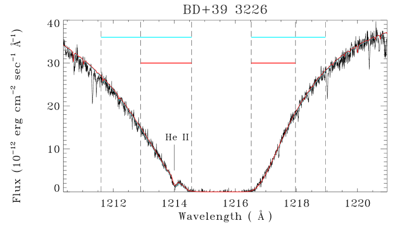
Figure 6.— A detailed view of the Ly$\alpha$ region of BD+39 3226. The meanings of the colors and dashed lines are the same as in Figure 2c. The red spectrum is almost indistinguishable from the cyan spectrum because $N$(H i) differs by only 0.006 dex between the two fits.

Continuum placement errors. The process for determining the best value of $N$(H i) minimizes the residual between the observed spectrum and the model spectrum. In the continuum region this is done by computing appropriate values of the coefficients of a 6th order polynomial. To estimate the contribution of continuum placement errors we compute the RMS deviation between the model and the observed spectrum in the continuum fitting regions and scale the model by this relative factor. We compute a new value of $N$(H i) with this fixed, high continuum, and then do the same with the similarly scaled low continuum placement (Figure 2b). The mean of the differences of these two values of $N$(H i) establishes the continuum placement error. This error ranges from 0.002 to 0.014 dex for LSE 234 and Feige 110 respectively. It is the largest source of error in $N$(H i) for five stars in our sample: Feige 110, CPD$-$71 172, LSE 263, BD+39 3226, and JL9. It may be surprising that the continuum contribution to the error is so small for LSE 234 (finale panel of Figure 4) when there is such an enormous deviation between the model and the spectrum on the red side of Ly$\alpha$. However, our continuum scaling region excludes 1226.2 to 1240.6Å for this object. More importantly, having one of the largest value of $N$(H i) in our target sample, the Ly$\alpha$ line has very well-developed damping wings, which renders our estimate of $N$(H i) quite insensitive to continuum placement errors. In other words, far out on the wings of the interstellar absorption profile there is a large covariance in the errors of the continuum level and the amount of H I. Near the core this is much less important. Thus, it is the core region which most strongly constrains the H I column density estimate.

Interstellar absorption velocity errors. We assume the interstellar absorption is from a single component at a single velocity. This velocity is common to H I and to low-ionization metals in the interstellar cloud, and is one of the free parameters determined as part of the $\chi^{2}$ minimization procedure. We determined the uncertainty in this velocity by measuring the velocities of metal lines such as Si II $\lambda\lambda 1193.3,1250.6$, N I $\lambda\lambda 1199.5,1200.2,1200.7$, and O I $\lambda\lambda 1302.2,1355.6$, when these lines are present and not too saturated. The RMS dispersion in the velocities of these lines provides a measure of the uncertainty in the velocity of the absorbing cloud. This velocity error was added to the best-fit interstellar velocity and then fixed during a new computation of $N$(H i). The RMS error estimate was then subtracted and the same procedure followed. The mean of the differences of the resulting values provided the error contribution to $N$(H i). It ranged from 0.0002 to 0.003 dex for JL9 and HD 41161, respectively, and is not the largest source of error for any target in our sample.

Table 3FUSE Observation Log

Target	Obs Date	Data ID	Exp. Time	$N_{\rm exp}$	Aperture
LB 1566	2003-07-15	P3020801	5.8	3	LWRS
	2003-09-11	P3020802	21.8	21	MDRS
LB 3241	2002-09-21	M1050301	9.1	17	LWRS
	2002-11-14	M1050302	5.6	11	LWRS
	2002-11-16	M1050303	11.1	22	LWRS
	2002-11-18	M1050304	9.7	19	LWRS
	2003-09-10	Z9040501	3.2	7	LWRS
LSE 263	2003-05-30	D0660401	4.0	8	MDRS
	2004-09-14	E0450201	23.1	32	MDRS
LSE 234	2003-04-07	P2051801	9.8	20	LWRS
	2003-05-30	P3021101	10.6	20	LWRS
	2006-04-22	U1093901	8.6	17	LWRS
CPD$-$71 172	2003-07-13	P3020201	11.4	25	MDRS

We note that the width of the Ly$\alpha$ line is more than 1300 km s^-1 (FWHM) for all sightlines, so large that any reasonable b-value has no discernible effect on the computed value of $N$(H i), and is therefore not included in our fit and does not materially contribute to the error.

Stellar model velocity errors. We bound the velocity uncertainty based on the width of the stellar lines. Typically, we find that shifts of approximately half the width of most stellar lines is the upper bound on the stellar velocity error. This was $\leq\pm$ 30 km s^-1 for the four OB stars and $\leq\pm$ 16 km s^-1 for the remaining stars. However, the error in $N$(H i) is highly insensitive to the stellar model velocity, and ranges from 0.0002 to 0.003 dex for HD 41161 and BD+39 3226, respectively, and is not the largest source of error for any target in our sample. This is expected since wings of the stellar H I absorption profile are so much narrower than the well developed damping wings of the interstellar H I profile.

Ly$\alpha$ fitting region errors. We showed in the previous section that the spectral location that most sensitively constrains $N$(H I) is about $\text@frac{1}{3}$ of the way up from zero flux to the full continuum level, but it is broad so it is best to use this spectral location plus some region on each side of it. However, we cannot always use this full range due to the presence of underlying stellar features that are not included in our model. The detailed selection of spectral region differs for each target. As an example, Figure 2(c) shows this region for WD1034+001. The red bars indicate the region used to compute $N$(H I). There is important information even just outside the core region so the inner extent of the red bars begins there. The bars extend to approximately 1213Å and 1218Å, corresponding to the peak sensitivity shown in Figure 3. In this case we do not extend them further due to some obvious absorption features in the spectrum.

To test the sensitivity to this choice, we performed the complete multi-parameter fit of $N$(H i) using a wider Ly$\alpha$ fitting region, shown by the horizontal cyan bars in Figure 2(c), with the best fit model spectrum also shown in cyan. For some targets this larger width included obvious discrepancies between the observed spectrum and the model but we accepted this to avoid underestimating the error associated with our nominal choice of width. A close examination of Figure 2(c) shows that the cyan spectrum lies largely below the observed (black) spectrum in the red bar region but the fit is better than the red one further from the core. This is because $N$(H i) is forced to increase in order to fit the wings of the Ly$\alpha$ profile over the wide (cyan) region. The red and cyan spectra have H I column densities of 20.119 and 20.142 dex, a difference of only 0.023 dex. Another example is shown in Figure 6, a detailed view of the Ly$\alpha$ region for BD39+3226, one of five targets observed at high resolution. In this case the red and cyan spectra are nearly indistinguishable, and correspond to $N$(H i) column densities of 20.011 and 20.017 dex respectively, a difference of only 0.006 dex. These examples demonstrate the exquisite quality of the data and the great sensitivity of $N$(H i) to the fit in the region just outside the Ly$\alpha$ core. The error associated with the selection of the width of the fitting region ranges from 0.00 (indicating that the standard and wide selections give the same value of $N$(H i)) to 0.016 dex for CPD$-$71 172 and LB 1566, respectively. The fitting region width is the largest source of error for PG0038+199, TD1 32709, WD1034+001, and LB 1566.

The discrepancy between the observed spectrum (black) and the best fit spectrum (red) for some targets shown in Figure 4 is forced by the need to not underestimate the continuum farther from the line core. The better fit in the upper wing region shown by the cyan spectrum comes at the penalty of a poorer fit near the bottom of the Ly$\alpha$ profile. Examination of Figure 4 shows that several other targets such as TD1 32709 and LB 1566, exhibit similar behavior to WD1034+001 to some degree. This effect has also been seen in the published profiles for PG0038+199 and WD1034+001 (Werner et al., 2017) and JL9 (Werner et al., 2022), so it is not unique to our fitting procedure.

Stellar model errors. In section 4 we described the stellar models we used to reproduce the observed spectra. Uncertainties in the stellar models can contribute to errors in the determination of $N$(H i). To assess the magnitude of this error for most targets we computed two extreme stellar models in which we changed the stellar atmospheric temperature and surface gravity to their maximum or minimum plausible values. We used our standard, 9 parameter fit to compute the best value of $N$(H i) for the pair of extreme cases, one leading to a low value and one leading to a high value of $N$(H i). The average of the difference between these values and the best value of $N$(H i) was the error associated with the stellar models. This error ranged from 0.001 to 0.015 dex for JL9 and LB 3241, respectively. The stellar model error is the largest contributor to the error in $N$(H i) for LSE 44 and LB 3241.

For the OB stars HD 41161, HD 90087, HD 53975, HD 191877 we did not compute extreme stellar models, because our static models do not take into account the strong P Cygni profiles in the N V doublet, which are observed on the red side of the Ly$\alpha$ line profile. For these 4 cases, to be conservative we adopted an error of twice the mean of the corresponding errors of the remaining 12 targets, or 0.012 dex.

6. New Measurements of $N$(D I)

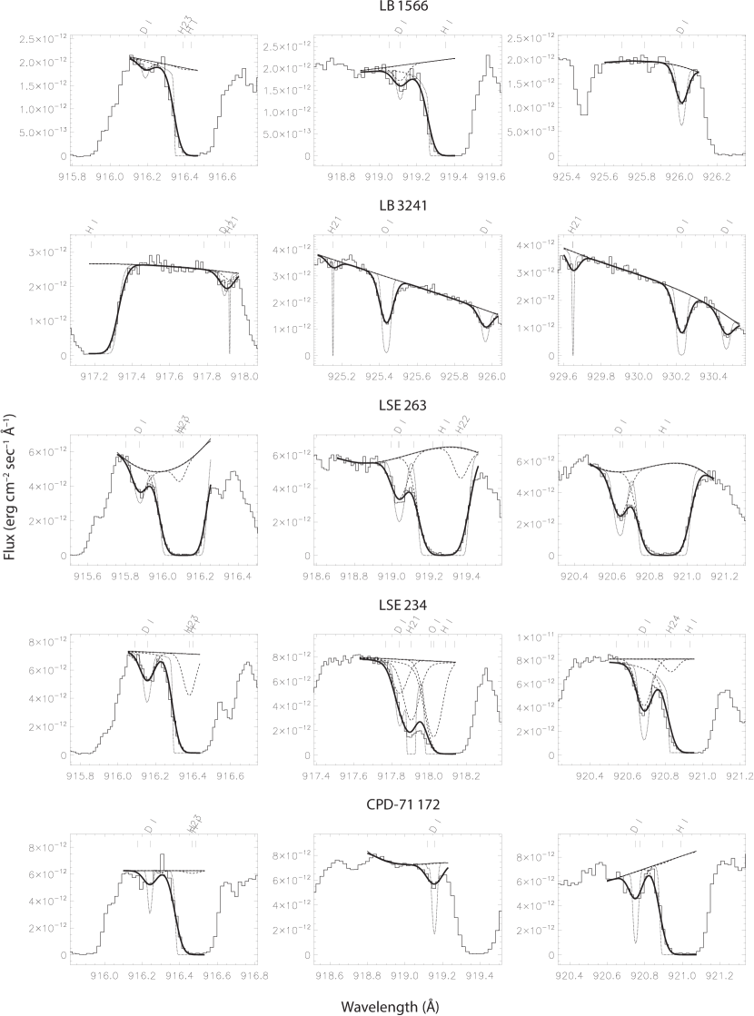
Figure 7.— Examples of FUSE spectral windows showing deuterium lines toward the five targets in this study without previously published values of $N$(D i). Histogram lines are the data, and the solid lines are continua and fits broadened by convolution with the FUSE LSF. The dashed lines are the fits for each species. The dotted lines are the model profiles prior to convolution with the LSF. The H₂ lines of the levels $J=1$ to $J=4$ are denoted as H21 to H24.

6.1. Observations and data processing

Five of our targets have no published $N$(D i) measurements: LB 1566, LB 3241, LSE 263, LSE 234, and CPD$-$71 172. All have archival FUSE data, with observations secured between 2002 and 2006, using the low or medium resolution slits, LWRS and MDRS, respectively (see Table 3). They were all obtained in histogram mode, except LB 3241 which was observed in time-tagged mode. We obtained from the FUSE archive the one-dimensional spectra, which were extracted from the two-dimensional detector images and calibrated using the CalFUSE pipeline (Dixon et al., 2007). The data from each channel and segment (SiC1A, SiC2B, etc.) were co-added separately for each of the two slits, after wavelength shift corrections of the individual calibrated exposures. Wavelength shifts between exposures were typically a few pixels. In the case of LB 1566 which was observed using both slits, the LWRS and MDRS data were co-added separately. The line spread function (LSF) and dispersions are different depending on the segments and the slits, thus requiring this separate treatment. These different datasets for a given target are used simultaneously but separately in the analysis reported below. The spectral resolution in the final spectra ranges between $\sim 13000$ and $\sim 18500$, depending on detector segment and wavelength. Clear D I Lyman series absorption lines are detected for all the targets.

6.2. Data analysis

The deuterium column densities $N$(D i) on the five lines of sight were measured by Voigt profiles fits of the interstellar spectral absorption lines. We used the profile fitting method presented in detail by Hébrard et al. (2002), which is based on the procedure Owens.f, developed by Martin Lemoine and the French FUSE Team (Lemoine et al., 2002). We split each spectrum into a series of small sub-spectra centered on absorption lines, and fitted them simultaneously with Voigt profiles using $\chi^{2}$ minimization. Each fit includes D I lines, as well as those of other species blended with them. Due to the redundancy of FUSE spectral coverage, a given transition might be observed in several segments and with one or two slits. These different observations allow some instrumental artifacts to be identified and possibly averaged out. The laboratory wavelengths and oscillator strengths are from Abgrall et al. (1993a, b) for molecular hydrogen, and from Morton (2003) for atoms and ions.

Several parameters are free to vary during the fitting procedure, including the column densities, the radial velocities of the interstellar clouds, their temperatures and turbulent velocities, and the shapes of the stellar continua, which are modeled by low order polynomials. Owens.f produces solutions that are coherent between all the fitted lines, assuming for each sightline one absorption component with a single radial velocity, temperature, and turbulence. Some instrumental parameters are also free to vary, including the flux background, the spectral shifts between the different spectral windows, or the widths of the Gaussian line spread functions used to convolve with the Voigt profiles. The simultaneous fit of numerous lines allows statistical and systematic errors to be reduced, especially those due to continuum placements, line spread function uncertainties, line blending, flux and wavelength calibrations, and atomic data uncertainties.

In Section 8 we present the complexity of the sight lines that we observed at high spectral resolution, particularly toward the most distant targets with numerous components present at different radial velocities. However, the velocity structure along these five lines of sight is not known and therefore we assumed a single interstellar component for each line. As discussed and tested in Hébrard et al. (2002), our measured column densities and their associated uncertainties are reliable with respect to this assumption, and they are also reliable considering typical temperature and turbulence of interstellar clouds, as well as the shape and width of the line spread function (LSF) of the observing instrument. Thus we report total deuterium column densities, integrated along each line of sight. The error bars were obtained using the $\Delta$$\chi^{2}$ method presented by Hébrard et al. (2002). The measured D I column densities are given in Table 4. Examples of the fits are shown in Figure 7.

Our measurements of $N$(D I) were derived from unsaturated lines. Saturated lines on the flat part of the curve of growth were excluded from consideration. We thus only kept the D I lines for which the model profiles prior to convolution with the LSF do not reach the zero flux level (see Figure 7). Indeed, saturated lines can introduce systematic errors on column density measurement (Hébrard et al., 2002; Hébrard & Moos, 2003). Issues related to saturation and other systematic effects were discussed extensively by Hébrard et al. (2002) and the method used here is exactly the same. In particular, Section 4.2 of that study discusses and tests the reliability of reported column densities and their uncertainties with respect to the number of interstellar clouds on the line of sight, their temperature and turbulence, and the shape and width of the LSF. The tests reported by Hébrard et al. (2002) show that the uncertainties on column densities are reliable when they are derived from the fit of unsaturated lines.

To exclude the saturated D I lines from our fits, we checked that their profiles prior to convolution with the LSF (shown as dotted lines in Figure 7) do not reach the zero flux level. The unconvolved profiles are constrained as numerous lines of several species are fitted simultaneously. For example, in the fit around 918Å of LSE 234 (fourth line, middle panel in Figure 7), the unconvolved profile appears to reach zero flux level but this is actually due to blending with a $J=1$ transition of molecular hydrogen. The D I transition is located $\sim$0.05Å to the blue side of this line. It does not reach the zero flux level and is not saturated, thus providing a reliable column density.

7. $N$(H i) and D/H Results

The principal results of this study are shown in Figure 8 and Table 4 where our new measurements of $N$(H i) are given in column 2. Column 3 lists the column densities of $N$(H₂). For the 7 targets with the TP code this was calculated using the method described in Section 3.2 of Jenkins (2019) who used the optical depth profiles created by McCandliss (2003). Column 4 shows our five new results of $N$(D i) presented in section 6 and for the remaining targets, previously published values. All measurements of $N$(D i) come from FUSE spectra. Column 5 gives our resulting values of D/H_tot, where $N$(H${}_{tot})$ = $N$(H i)+2$N$(H₂). 2$N$(H₂) is a relatively minor constituent of $N$(H${}_{tot})$, ranging from 15.9% down to 7.0% for HD 191877, PG 0038+199, HD 41161, HD 90087, JL 9, and less than 3.5% for the remaining 11 stars in our sample. We can ignore the presence of HD in our assessment of the deuterium abundance, since $N({\rm HD})$ is generally of order $3\times 10^{-7}N({\rm H_{tot}})$ (Snow et al. 2008).

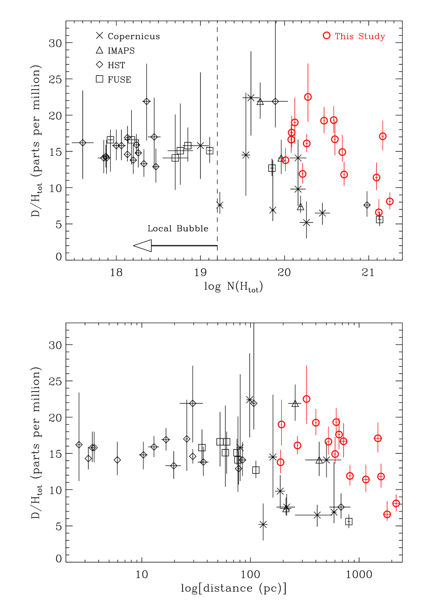
Figure 8.— Top: D/H_tot vs. log($N$(H${}_{tot})$), where $N$(H${}_{tot})$= $N$(H i) + 2$N$(H₂) is the total neutral and molecular hydrogen column density. $N$(H i) is used if $N$(H${}_{tot})$ is not available. The red symbols are from this study. The symbols for the other data points designate the spacecraft that observed the line of sight. The boundary of the Local Bubble, taken to be at log($N$(H${}_{tot})$) = 19.2, is shown as the vertical dashed line. Bottom: D/H_tot vs. distance. Distances are from Gaia and Hipparcos.

Table 4The column densities of neutral hydrogen, molecular hydrogen, neutral deuterium, and D/H${}_{tot}^{\rm a}$

Target	log($N$(H i))	log($N$(H2))	log($N$(D i))	D/Htot	Referencesb
BD+39 3226	$20.01\pm 0.01$	$15.65^{+0.06}_{-0.07}$	$15.15\pm 0.05$	$13.78^{+1.71}_{-1.53}$	O++06, O++06
TD1 32709	$20.08\pm 0.01$	$14.48^{+0.12}_{-0.11}$	$15.30\pm 0.05$	$16.63^{+2.08}_{-1.86}$	O++06, O++06
LB 3241	$20.08\pm 0.02$	$14.50^{+0.30}_{-0.50}$	$15.33\pm 0.05$	$17.60^{+2.27}_{-2.04}$	TP, TP
WD 1034+001	$20.12\pm 0.02$	$15.72^{+0.13}_{-0.12}$	$15.40\pm 0.07$	$19.00^{+3.39}_{-2.91}$	O++06, O++06
LB 1566	$20.21\pm 0.01$	$15.48^{+0.18}_{-0.18}$	$15.29\pm 0.05$	$11.90^{+1.49}_{-1.33}$	TP, TP
Feige 110	$20.26\pm 0.02$	$15.20^{+0.30}_{-0.40}$	$15.47\pm 0.03$	$16.10^{+1.28}_{-1.20}$	TP, F++02
CPD$-$71 172	$20.28\pm 0.01$	$15.60^{+1.10}_{-0.35}$	$15.63^{+0.08}_{-0.07}$	$22.51^{+4.61}_{-3.43}$	TP, TP
PG 0038+199	$20.40\pm 0.01$	$19.33^{+0.02}_{-0.02}$	$15.75\pm 0.04$	$19.24^{+1.89}_{-1.73}$	W++05, W++05
LSE 44	$20.57\pm 0.01$	$18.82^{+0.10}_{-0.10}$	$15.87\pm 0.04$	$19.31^{+1.94}_{-1.78}$	TP, F++06
LSE 263	$20.60\pm 0.01$	$16.40^{+0.40}_{-0.50}$	$15.82\pm 0.06$	$16.68^{+2.51}_{-2.20}$	TP, TP
JL 9	$20.68\pm 0.01$	$19.25^{+0.02}_{-0.02}$	$15.78\pm 0.06$	$11.81^{+1.77}_{-1.54}$	W++04, W++04
LSE 234	$20.69\pm 0.01$	$16.35^{+0.25}_{-0.35}$	$15.86^{+0.06}_{-0.04}$	$14.91^{+2.35}_{-1.33}$	TP, TP
HD 191877	$21.05\pm 0.02$	$20.02^{+0.05}_{-0.05}$	$15.94^{+0.11}_{-0.06}$	$6.60^{+1.82}_{-0.88}$	SDA21, H++03
HD 53975	$21.08\pm 0.02$	$19.18^{+0.04}_{-0.04}$	$16.15^{+0.07}_{-0.07}$	$11.40^{+2.04}_{-1.74}$	OH06, OH06
HD 41161	$21.10\pm 0.02$	$20.02\pm{0.03}$	$16.40^{+0.05}_{-0.05}$	$17.30^{+2.24}_{-2.01}$	SDA21, OH06
HD 90087	$21.21\pm 0.02$	$19.91\pm{0.03}$	$16.16^{+0.06}_{-0.06}$	$8.09^{+1.23}_{-1.08}$	SDA21, H++05

Our values of D/H_tot as a function of $N$(H${}_{tot})$ are plotted in Figure 8 together with previously reported measurements made with data from Copernicus, IMAPS, HST, and FUSE. This figure may be compared directly to Figure 1 in L06. Note that the figures differ slightly in that we plot D/H_tot vs. H_tot while they plot D/H I vs. H I. We also plot D/H_tot vs distance. Distances are taken from Gaia DR3 (Soszyński, 2016; Vallenari et al., 2022) when available (38 stars) and Hipparcos (Perryman, 1997) when not (15 stars).

The primary question we sought to answer in this study is whether the previous determinations of D/H_tot seen in targets beyond the Local Bubble are due to errors in the measured values of $N$(H i). It is now clear that this is not the case. The 16 new values of D/H_tot are not consistent with a single value of the deuterium abundance. In fact, the best straight line fit through these points without constraining the slope yields $\chi^{2}$ = 57 and the probability that a linear fit would give this value or greater is $4\times 10^{-7}.$ However, the scatter of the points is now substantially reduced compared to previous determinations. The standard deviation of D/H_tot for the 16 targets in our study is 4.3 ppm, compared to 6.0 ppm in L06 for the 9 targets that are common to both studies, despite the fact that the means of the distributions are almost unchanged at 15.2 and 15.7 ppm, respectively. Including $N$(H i) values from Diplas & Savage (1994) we find the interesting result that 11 of the 13 points with both old and new published values of D/H_tot moved closer to the mean. That is to say, the high points moved lower and the low points moved higher. The typical change is $1-2\sigma$ which for an individual point would not be noteworthy but perhaps is for such a large majority of points. The exceptions are HD191877 and HD90087, which moved 0.9 $\sigma$ and 1.0 $\sigma$ away from the mean, respectively. We have identified no systematic effect which may be responsible for this general trend toward the mean.

With the recent Gaia DR3 data release most of the distances to our targets are now known to high accuracy and in the bottom of Figure 8 we plot D/H_tot vs. distance. Since we found greater scatter in D/H_tot at large values of $N$(H${}_{tot})$, we expected to see a similar scatter at large distances. The plot shows exactly this result with no particular trend with distance other than approximate constant D/H_tot within $\sim 100$ pc, as was previously known. This is consistent with estimates of the distance to the wall of the Local Bubble ranging from $65-250$ pc, depending on direction (Sfeir et al., 1999).

8. Measurement of Metal Abundances

Our observations permit a detailed analysis of metal abundances toward the five targets for which we obtained high resolution echelle data. We discuss the analysis and results in this section.

The metal lines for the stars observed at high resolution, HD 191877, HD 41161, HD 53975, HD 90087 and BD+39 3226, were fitted with vpfit 9.5 (Carswell & Webb, 2014). Table A1 in Appendix A shows the sources of the f-values we used. In addition to the basic wavelength and flux vectors from the datasets listed in Table 1, we used the associated 1$\sigma$ error arrays, and created continua using a semi-manual method. We first employed a 15 pixel median filter for a rough continuum estimate, then fitted around the lines using either a series of linear interpolations, selected to connect the median-filtered curves over absorption lines, or the IRAF continuum package (Tody, 1986, 1993) around more complex regions.

The $1\sigma$ error arrays were then verified for consistency with the root mean square (rms) variations for the normalized (flux/continuum) vectors. The check was done for all bin values from 5 to 1000 pixels. Deviations from rms values were typically on the order of 10-20%. We made a correction in vpfit parameter files to employ this correction, though in certain wavelength intervals, particularly in line troughs, larger correction factors sometimes had to be employed. This reflected a combination of systematic errors which may not have been completely accounted for in the HST pipeline reductions, and also under-sampling of the LSF when using grating E140H with the Jenkins slit ($0.1^{\prime\prime}\times 0.03^{\prime\prime}$). (We did not request any special detector half-pixel sampling with the observations, which would be necessary to exploit the full resolving power of this slit.)

For the profile fits with vpfit, we employed the library STScI LSF for the given grating and slit combination. We generally required a probability of the fitted profiles being consistent with the data of at least $p=0.01$, as a goodness of fit threshold. In some cases, we tied the radial velocities of several ions together, to make multiple simultaneous fits. Also in some cases, we allowed a linear offset of the continuum level as a free parameter, which effectively compensates for unidentified line blends with other ions, though this was in a small minority of cases. Finally, due either to the under-sampled LSF, noise spikes, or potential artifacts in the reduced spectra, we occasionally increased the error values by factors up to 2-3 to reduce the effects of individual pixels on the fits and obtain acceptable statistical fits.

Detailed notes on individual objects are presented in Appendix A along with column density and other observational data for each sight line.

9. Correlation with Depletions of Heavy Elements

There have been numerous studies that compared D/H measurements with the relative abundances of other elements (Prochaska et al. 2005; Linsky et al. 2006; Oliveira et al. 2006; Ellison et al. 2007; Lallement et al. 2008), in order to investigate the hypothesis that D more easily binds to dust grains than H, as suggested by Jura (1982), Draine (2004, 2006), and Chaabouni et al. (2012). All have shown that there are correlations between D/H and gas-phase abundances of certain elements that exhibit measurable depletions onto dust grains in the interstellar medium. While these correlations are statistically significant and reinforce the picture that the more dust-rich regions have lower deuterium abundances, the scatters about the trend lines are larger than what one could expect from observational errors.

In this section, we investigate this issue once again, including not only our own data but also results reported elsewhere. However, our analysis here incorporates two important differences in approach from the earlier studies. First, we characterize the depletions of heavy elements in terms of a generalized depletion parameter $F_{*}$ developed by (Jenkins, 2009, 2013). The use of $F_{*}$ instead of the depletion of a specific element allows us to include in a single correlation analysis the data for cases where the depletion of any element is available instead of just one specific element. Moreover, if for any given case more than one element has had its column density measured, the results will effectively be averaged, yielding a more accurate evaluation of the strength of depletion by dust formation. A second important aspect of our study is that we limit the results to cases where $\log N({\rm H_{tot}})=\log[N({\rm H~{}I})+2N({\rm H}_{2})]>19.5$, following a criterion defined by Jenkins (2004, 2009), so that we can reduce the chance that the abundance measurements are distorted by ionizations caused by energetic starlight photons that can penetrate part or much of the H I region(s) (Howk & Sembach 1999; Izotov et al. 2001).

Much of the information about heavy element column densities is taken from the compilation of Jenkins (2009), with its specific standards for quality control and adjustments for revised transition $f$-values. We have added a few new determinations that came out later in the literature. An evaluation of $F_{*}$ for any individual element $X$ is given by the relation,

$$F_{*}(X)={\log N(X)-\log N({\rm H_{tot}})-(X/{\rm H})_{\odot}-B_{X}\over A_{X}}+z_{X}~{},$$ (1)

where the constants $(X/{\rm H})_{\odot}$, $A_{X}$, $B_{X}$, and $z_{X}$ are specified for each element in Table 4 of Jenkins (2009). We can arrive at an error in $F_{*}(X)$ by using Geary’s (1930) prescription for the error of a quotient for an expression $N/D$ (numerator over denominator),

$$\sigma(Q)=\sigma\left[{N\pm\sigma(N)\over D\pm\sigma(D)}\right]$$ (2)

with

$$\sigma(N)=\{\sigma[\log N(X)]^{2}+\sigma[\log N({\rm H_{tot}})]^{2}+\sigma[B_{\rm red}]^{2}\}^{1/2}$$ (3)

and

$$\sigma(D)=\sigma(A_{X})~{}.$$ (4)

The error in the $B_{X}$ term in Eq. 1 is a reduced form

$$\sigma[B_{\rm red}]=\{\sigma(B_{X})^{2}-\sigma[(X/{\rm H})_{\odot}]^{2}\}^{1/2}$$ (5)

because any uncertainty in the solar abundance $(X/{\rm H})_{\odot}$ has no effect on the outcome for $F_{*}$; $B_{X}$ would change by an equal amount in the opposite direction. Put differently, $\sigma[B_{\rm red}]$ represents just the uncertainty in the original fit without the systematic error from $(X/{\rm H})_{\odot}$. There is no error in $z_{x}$; this constant is used to insure that the error in $A_{X}$ is uncorrelated with that of $B_{X}$. Ultimately, we use $\sigma(Q)$ as the value for the uncertainty in $F_{*}(X)$.

Table B1 lists the data that were assembled for constructing the correlation, and Table B2 indicates the sources in the literature that led to the values shown by the codes listed in Table B1. For each sight line, a weighted average for $F_{*}$ over all elements $X$ was determined from

$$\langle F_{*}\rangle=\sum_{X}F_{*}(X)\sigma[F_{*}(X)]^{-2}\Bigg{/}\sum_{X}\sigma[(F_{*}(X)]^{-2}~{},$$ (6)

where the error in this quantity is given by

$$\sigma[\langle F_{*}\rangle]=\left[\sum_{X}\sigma[(F_{*}(X)]^{-2}\right]^{-1/2}~{}.$$ (7)

For the elements C, N and Kr, $\sigma(A_{X})>A_{X}/3$, which makes $\sigma(Q)$ in Eq. 2 untrustworthy (and the errors large). Results for these three elements were ignored and not included in Table B1. Figure 9 shows $\log[N({\rm D~{}I})/N({\rm H_{tot}})]$ as a function of $\langle F_{*}\rangle$. As noted above, we can ignore the presence of HD in our assessment of the deuterium abundance. $\langle F_{*}\rangle$ for LSE 44 was determined from only the abundance of oxygen; the error here is so large that this case was not included in the analysis or the plot.

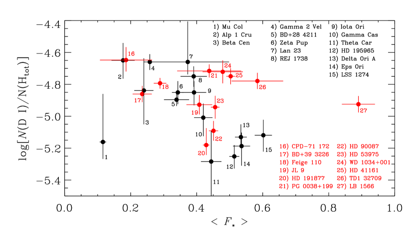
Figure 9.— The relationship between $\log[N({\rm D~{}I})/N({\rm H_{tot}})]$ and the generalized depletion parameter $\langle F_{*}\rangle$ for our determinations (in red) and others from data in the literature (in black), as listed in Table B1.

To assess whether or not the D/H and metal depletion measurements in Figure 9 are anticorrelated (note that as depletion becomes more severe it becomes more negative), we begin with nonparametric Spearman and Kendall $\tau$ correlation tests. Using all of the data in Figure 9, we find a Spearman correlation coefficient $r_{s}=-0.42$ with a $p-$value of 0.028, and we obtain a Kendall $\tau=-0.32$ with $p-$value = 0.021. Both of these tests indicate that the data are weakly correlated at slightly better than 2$\sigma$ significance. This is similar to results obtained in previous studies, although we note that L06 did not find a significant correlation in their sample with log $N$(H I) $>$ 19.2 (i.e., their sample that most closely matches the criteria we have used to select our sample). We have reduced the uncertainties of some of the measurements in L06 and we have added new sightlines; evidently these improvements have revealed a weak correlation even in this higher-$N$(H I) sample.

This correlation may be slightly misleading, since both variables in Figure 9 have experimental errors that are partly composed of errors of a single quantity, $\log N({\rm H_{tot}})$. In our comparison shown in Figure 9, the $y$ values are driven in a negative direction by positive errors in $\log N({\rm H_{tot}})$, while the reverse is true for the $x$ values (see Eq. 1), since for most elements $A_{X}\approx-1$. Hence, measurement errors in $\log N({\rm H_{tot}})$ will artificially enhance the magnitude of the negative correlation over its true value in the absence of such errors. To investigate this concern, we have carried out two additional tests that are less vulnerable to this problem. As we discuss in the next two paragraphs, these two additional tests further support the finding that D/H is weakly correlated with metal depletion.

First, we have examined whether $N$(D I)/$N$(Fe II) is correlated with $\log N({\rm H_{tot}})$. Iron depletion is typically strongly correlated with $\log N({\rm H_{tot}})$ because sightlines with higher $\log N({\rm H_{tot}})$ tend to have higher gas densities, higher molecular-hydrogen fractions, and physical conditions that are more conducive to elemental depletion by dust. Using the data in Figure 9, the Spearman test comparing iron depletion vs. $\log N({\rm H_{tot}})$ yields $r_{s}=-0.67$ with $p-$value = 0.0001, which confirms that Fe depletion is correlated with the hydrogen column in these data. Therefore if the deuterium abundance is not correlated with iron depletion, then $N$(D I)/$N$(Fe II) vs. $\log N({\rm H_{tot}})$ should be correlated with a positive slope — as $\log N({\rm H_{tot}})$ increases and the relative iron abundance decreases due to depletion, $N$(D I)/$N$(Fe II) should go up. This is not what we observe. Instead, we find no correlation between $N$(D I)/$N$(Fe II) and $\log N({\rm H_{tot}})$ (Spearman $r_{s}=0.11$ with $p-$value = 0.58), which suggests that as the relative abundance of Fe decreases, the deuterium abundance decreases accordingly so that $N$ (D I)/$N$(Fe II) stays more or less the same. A linear fit to $N$(D I)/$N$(Fe II) vs. $\log N({\rm H_{tot}})$ has a slope consistent with zero within the errors ($m=2.1\pm 3.6$). We note that there is substantial scatter in $N$(D I)/$N$(Fe II) vs. $\log N({\rm H_{tot}})$, just as there is substantial scatter in Figure 9.

Second, we have split the data in Figure 9 into two equal-sized bins, one with lower amounts of metal depletion and one with higher depletions, and we have compared the D/H distributions in each bin. Figure 10 overplots the resulting D/H distributions for the data with $\langle F_{*}\rangle\leq 0.42$ (lower metal depletion) vs. the data with $\langle F_{*}\rangle>0.42$ (greater metal depletion). Applying a Kolmogorov-Smirnov (KS) test to the two samples shown in Figure 10, we find the KS statistic $D=$ 0.48 with $p-$value = 0.062. This only tentatively rejects the null hypothesis (that the distributions are drawn from the same parent distribution) at slightly less than 2$\sigma$ confidence. However, the only criterion used to choose $\langle F_{*}\rangle$ = 0.42 to delineate the “low-depletion” and “high-depletion” samples is that it divides the data into two (almost) equal halves, and this results in 14 data points in the low-depletion bin and 13 points in the high-depletion bin. One of the measurements is right on the $\langle F_{*}\rangle$ = 0.42 boundary and has a low D/H ratio; if we change the definition slightly by placing all points with $\langle F_{*}\rangle\geq 0.42$ in the high-depletion group (resulting in 13 points in the low-depletion bin and 14 in the high-depletion bin), the KS test changes to $D$ = 0.57 with $p-$value = 0.015. Clearly more D/H and depletion measurements would be helpful. The Anderson-Darling (AD) two-sample test, which can be applied in the same way as the KS test but may be more effective in some situations (Engmann & Cousineau, 2011), returns $p-$value = 0.023 and 0.012 in comparisons of the samples with number of low/high depletion points = 14/13 and 13/14, respectively. The AD test therefore indicates that the low-depletion and high- depletion samples are different at a slightly better significance, but nevertheless all of these tests provide weak indications that the distributions of D/H ratios are different when the metal-depletion level is low or high.

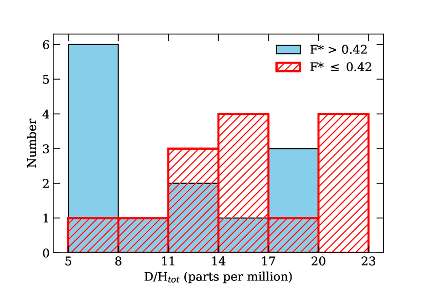
Figure 10.— Comparison of D/H_tot distributions from the sightlines studied here, split into two samples: the sightlines with low metal depletion ($\langle F_{*}\rangle\leq 0.42$, red-hatched histogram) and the sightlines with higher metal depletion ($\langle F_{*}\rangle>0.42$, solid-blue histogram).

We have conservatively required our D/H sample to have log $N$(H I) $\geq$ 19.5 to avoid systematic confusion from ionization effects. This is a reasonable threshold for distant sightlines that may probe regions with high starlight intensities and high ionization parameters, which can elevate the contribution of ionized gas along a sightline. However, inside the Local Bubble, the ionizing radiation field and ISM gas physics have been studied in detail (e.g., Redfield & Linsky, 2008; Frisch et al., 2011), and while there are uncertainties, inside the Local Bubble the ionization parameter is likely quite low (Slavin & Frisch, 2002), and Local Bubble sightlines with log $N$(H I) $\geq$ 18.0 will have iron ionization corrections less than 0.15 dex (see Fig.6 in Lehner et al., 2003). Therefore we can add Local Bubble sightlines from L06 with log $N$(H I) $\geq$ 18.0 without introducing appreciable error from ionization corrections. If we combine our data with the 13 Local Bubble sightlines from L06 with log $N$(H I) $\geq$ 18.0 that have Fe depletion measurements, we find a similar result with somewhat better significance: a Spearman test for D/H vs. [Fe/H] including the Local Bubble gives $r_{s}$ = 0.39 with $p-$value = 0.014. Of course, this gives the Local Bubble, where D/H is fairly uniform and the metal depletion is relatively low, considerable weight, but it is interesting that even with this significant increase in the overall sample size, the resulting correlation is not very strong.

In Figure 9 there appears to be a bifurcation of D/${\rm H_{tot}}$ values for $\langle F_{*}\rangle>0.4$. L06 noted a similar separation, but with a slightly different selection of target stars and using the depletion of Fe instead of $\langle F_{*}\rangle$ as a discriminant. If this effect is real and not a product of random processes, can we devise a possible explanation? L06 proposed that differences in grain properties could explain this phenomenon. We think that an alternate interpretation is possible. As we mentioned in Section 1, there is evidence that low-metallicity gas in the Galactic halo has a higher than usual deuterium fraction. When this gas mixes with material at the upper or lower boundaries of the Galactic plane gas, it might modify the D/H to higher values without appreciably changing the apparent values of $F_{*}$. We could test this proposition by examining whether or not the high and low branches of the D/${\rm H_{tot}}$ trends shown in Figure 9 have significant differences in the distances $|z|$ of the target stars from the Galactic plane. Table 5 shows the $|z|$ values for stars in the two groups.

While the high group has an average $|z|$ equal to 343 pc and the low group has an average $|z|$ equal to 160 pc, it is not clear that these differences are significant. In order to test the proposition that these outcomes represent separate populations in $|z|$, we performed a KS test, and it revealed that there was a 5% probability that the two populations were drawn from a single parent distribution. We also performed an AD test which gave a p-value for the null hypothesis of 0.026, corresponding to a $2\sigma-3\sigma$ significance. Thus, at only a modest significance level, we suggest that $|z|$ is a possible discriminant for the two branches in D/H_tot for sight lines that exhibit moderate to high depletions of heavy elements. We propose that less dust in the infalling gas means that the freeze out of deuterium would be reduced, which may add to the effect of this gas having had less destruction of deuterium by astration.

Table 5Distances from the Galactic Plane for Stars with $\langle F_{*}\rangle>0.4$

Low D/${\rm H_{tot}}$			High D/${\rm H_{tot}}$
Star	$|z|$		Star	$|z|$
	(pc)			(pc)
HD 191877	203		PG0038 +199	271
HD 90087	80		WD1034 +001	142
HD 53975	46		HD 41161	332
JL9	722		TD1 32709	245
HD 36486	64		LB 1566	726
HD 37128	179
HD 93030	12
HD 195965	72
LSS 1274	63

10. Discussion

While it has long been known that the measured values of D/H along many sightlines within the Local Bubble are consistent with a single value (Linsky, 1998; Moos et al., 2002; Hébrard & Moos, 2003), beyond this structure the measurements show variability. The primary goal of this study is to determine whether this variability was the result of errors in the relatively poorly measured values of H I column density. With this study we have more firmly established that the variability is real but slightly smaller than previously estimated.

L06 suggested there are three separate regimes of D/H values each defined by a range of H I column densities (see their Figure 1). The first spans log $N$(H) $<19.2$, which is approximately the range within the Local Bubble and was chosen because D/H is constant within this limit. Here they find (D/H)${}_{LB}=15.6\pm 0.4$ ppm for 23 sight lines where the uncertainty is the standard deviation in the mean. The highest column density range corresponds to log N(H I) $>20.7$ where again they note that D/H is approximately constant and, notably, lower than (D/H)${}_{LB}.$ In this regime they found D/H${}_{dist}=8.6\pm 0.8$ ppm (standard deviation in the mean) for 5 sight lines toward the most distant targets (HD 90087, HD 191877, LSS 1274, HD 195965, and JL 9). The standard deviation of the D/H values is 0.95 ppm. In the intermediate regime, 19.2 $\leq$ $N$(H) $\leq$ 20.7, D/H is highly variable spanning a range from $5.0^{+2.9}_{-1.4}$ for $\theta$ Car to $22.4^{+11.7}_{-6.2}$ for LSE 44 or, selecting a target with much smaller errors, $21.8\pm 2.1$ for $\gamma^{2}$ Vel.

Our study did not include any targets in the first regime. However, our new results do not support the idea the D/H is constant in the most distant regime. We have computed revised values of $N$(H i) for HD 90087, HD 191877, and JL 9; see Table 4. Combining our new values of D/H with those in L06 for LSS 1274 and HD 195965 gives D/H${}_{dist}=8.3\pm 0.7$ (standard deviation in the mean) with a standard deviation of D/H of 2.0 ppm. This dispersion is more than twice L06 value. The targets most responsible for this increase in scatter are HD 41161 and HD 53975, neither of which was in the L06 study. And for JL 9, due to the decrease in our estimate of log $N$(H i) from $20.78\pm 0.05$ to $20.68\pm 0.009$, this star would not formally be included in the 3rd (highest H I column density) regime.

If we continue with the same $N$(H) criteria for the 3rd regime, we now have 6 stars that qualify: LSS 1274, HD 191877, HD 53975, HD 41161, HD 195965, and HD 90087, four of which have been revised or are newly determined in this study. These have a mean of 7.9 ppm and a standard deviation of 4.8 ppm. In the intermediate region our study has 25 sight lines with a mean of 13.0 ppm and a standard deviation of 5.3 ppm. There is no statistical distinction between the intermediate and distant regions, suggesting that similar physical processes are responsible for the distribution of D/H values in both regimes.

There is another simple way to compare the gas inside and outside the LB. For the group of 22 target stars shown in Figure 8 that lie within the LB we compute the sum of all $N$(D i) values and the sum of all $N$(H${}_{tot})$ values, and take the ratio of these group sums. We compute the identical sums and ratio for the 31 points outside the LB. The results are 15.4 ppm and 11.3 ppm, respectively, which are consistent with idea that high $N$(H${}_{tot})$ sight lines have higher $F_{*}$ and that D/H_tot decreases as $F_{*}$ increases. Based on the D abundance, this shows in a general way that the material in the LB is not simply a homogenized sample of material found at greater distances.

Comparisons of present-day Milky Way abundances to observations of three primordial species can be used to constrain models of Galactic chemical evolution. First, emission lines from H II regions in low metallicity star-forming galaxies yield the mass fraction of ⁴He (Izotov et al., 2014; Aver et al., 2015). Second, the ⁷Li abundance has been measured in the atmospheres of metal-poor stars (Spordone et al., 2010). Third, and most relevant to this study, quasar absorption line observations of clouds with extremely low metallicity give the D/H ratio in gas that is as close to pristine as possible (Burles & Tytler, 1998a, b; Kirkman et al., 2003; Cooke et al., 2014, 2016, 2018). Zavarygin et al. (2018) computed a weighted average of 13 high quality D/H measurements in QSO absorption line systems as D/H${}_{prim}=25.45\pm 0.25$ ppm. The highest precision measurement is (D/H)${}_{prim}=25.27\pm 0.30$ ppm (Cooke et al., 2018) in a system with an oxygen abundance [O/H] = $-2.769\pm 0.028$, or about 1/600 of the solar abundance. Approaching this in a different way, using improved experimental reaction rates of $d(p,\gamma)^{3}$He, $d(d,n)^{3}$He, and $d(d,p)^{3}$H, Pitrou et al. (2021) theoretically calculate the primordial ratio as (D/H)${}_{prim}=24.39\pm 0.37,$ about 2.1$\sigma$ below the quasar measurements. Similarly, Pisanti et al. (2021) find (D/H)${}_{prim}=25.1\pm 0.6\pm 0.3$, where the two errors are due to uncertainties in the nuclear rates and baryon density, respectively. This agrees very well with the measured value. For the purpose of comparing to the local values of D/H in our study we prefer to be guided by the experimental values of Zavarygin et al. (2018) and Cooke et al. (2018) and take (D/H)${}_{prim}=25.4\pm 0.3$ ppm.

In order to constrain models of Galactic chemical evolution, we want to compare (D/H)_prim to the total deuterium abundance in the Galaxy. As noted in section 1 there are two effects that could complicate assessing the total deuterium abundance. First, low metallicity gas may still be accreting onto the disk of the Milky Way. This gas may have a higher D/H ratio than gas in the ISM that has been polluted by material processed in stellar interiors and expelled via stellar winds and supernovae. Sembach et al. (2004) showed that the high velocity cloud Complex C is falling into the Galaxy and has D/H = $22\pm 7$ ppm. Savage et al. (2007) measured the deuterium abundance in the warm neutral medium of the lower Galactic halo and found D/H = $22^{+8}_{-6}$ ppm, virtually the same as in Complex C. Some of our sight lines have D/H values even greater than this, but note that the Complex C and the neutral medium measurements have large error bars. Our results provide some support for the infall hypothesis as the possible cause of the bifurcation of points in Figure 9 at higher levels of depletion, $\langle F_{*}\rangle>0.4.$ This D-rich material likely has low dust content reducing available sites for deuterium depletion. More recently, by stacking spectra of many background QSOs to increase the sensitivity to high velocity clouds, Clark, Bordoloi, & Fox (2022) show that infalling gas tends to be in small, well-defined structures with angular scales $\theta<40\arcdeg.$ Observed metallicities range from 0.1 solar (Wakker et al., 1999) to solar (Richter et al., 2001; Fox et al., 2016). This patchiness may well be responsible for some of the observed variability in D/H reported here.

As noted earlier, one would expect an anticorrelation between gas-phase metal abundance and D/H which does not appear to be the case (Hébrard & Moos, 2003). The second effect is while we assume that hydrogen depletion onto dust grains is negligible (Prodanović, Steigman, & Fields, 2010), the depletion of D onto the surfaces of dust grains (Draine, 2004, 2006) removes a fraction of the D from the gas phase that is measured in absorption line studies. In this case we expect a correlation between metal abundance and D/H (Prochaska et al., 2005; Ellison et al., 2007; Lallement et al., 2008). Prodanović, Steigman, & Fields (2010) note that while strong shocks would liberate both D and Fe, weaker shocks would liberate D only since it is weakly bound to dust mantles while Fe is locked in grain cores. Our results only show a potentially weak anti-correlation between the D/H and $\langle F_{*}\rangle$, adding weight to the conclusion that depletion onto dust grains is not always the dominant factor and that the local sight line history needs be considered. This may be responsible for some of the scatter in this correlation.

On the basis of several arguments including the metal abundance correlation, high D/H ratios observed in interplanetary dust particles believed to originate in the ISM, and the effects of unresolved but saturated D lines, L06 conclude that the large variation of D/H values beyond the Local Bubble are due to variable D depletion along different lines of sight. They called attention to 5 stars ($\gamma^{2}$ Vel, Lan 23, WD1034+001, Feige 110, and LSE 44) outside the Local Bubble that had high D/H values, ranging from 21.4 to 22.4 ppm. They stated that the total local Galactic D/H must be $\approx 22$ ppm or slightly greater.

In this study we have reevaluated $N$(H) of three of these stars resulting in improved estimates of D/H, all to lower values: WD1034+001 from $21.4\pm 5.3$ to $19.00^{+3.39}_{-2.91}$; Feige 110 from $21.4^{+5.7}_{-3.8}$ to $16.10^{+1.28}_{-1.20}$; and LSE 44 from $22.4^{+11.7}_{-6.6}$ to $19.31^{+1.94}_{-1.78}$. Ignoring Lan 23 due to its large errors, there are now three stars with high D/H: $\gamma^{2}$ Vel at $21.9^{+2.6}_{-2.4}$, $\alpha$ Cru at $22.4^{+6.4}_{-5.2}$, and a new one from this study, CPD$-$71 172 at $22.51^{+4.61}_{-3.43}$ the average of which, $\approx 22.1$, is almost the same as L06 estimated. However, Prodanović, Steigman, & Fields (2010) point out the potential bias introduced when selecting only a small number of high D/H values to consider when there are many other lower deuterium abundances that are consistent with these within the errors. They used a more sophisticated Bayesian approach to estimate the undepleted abundance in the local ISM using the 49 lines of sight in L06 and concluded that (D/H)${}_{undepleted}=20\pm 1$ ppm. In their analysis they used a “top-hat” shaped prior for D/H, which is the least model-dependent of those they considered, although they also modeled 4 others including positive and negative biased priors. Our new results as shown in Figure 8 actually correspond to this unbiased prior better than the L06 data because the values of D/H in our study are more uniformly distributed. For example, for log $N$(H)$\geq 20.7$ we have 6 targets with D/H ranging from $5.6-17.3$ ppm. L06 have 5 targets ranging from $7.6-10$ ppm. Thus, we adopt the Prodanović, Steigman, & Fields (2010) value of (D/H)_undepleted and using the current value of (D/H)_prim discussed above we find an astration factor $f\rm_{D}=(25.4\pm 0.3)/(20\pm 1)=1.27\pm 0.07.$ This may be compared to the values reported by L06 of $f\rm_{D}\leq 1.19^{+0.16}_{-0.15}$ and $f\rm_{D}\leq 1.12\pm 0.14$, depending on which value of (D/H)_prim they used. Thus, while marginally higher, our astration factor does not significantly differ from either of the L06 estimates.

We remind the reader that this may not represent the D/H value throughout the Galaxy (Lubowich & Pasachoff, 2010; Leitner & Kravtsov, 2011; Lagarde et al., 2012).

We now briefly consider this astration result in the context of models of Galactic chemical evolution in the Milky Way. As previously noted, the gas-phase deuterium abundance can be enhanced by the local infall onto the Galactic disk of primordial or at least less processed gas having low metallicity. Several investigators conclude that this and other mechanisms are necessary to account for the low value of $f\rm_{D}$ found by L06. Tsujimoto (2011) argues that this result is due to the decline in the star formation rate in the last several Gyr which has suppressed astration over this same period. Prodanović & Fields (2008) make a strong case for Galactic infall (the very title of their paper) by showing that such small $f\rm_{D}$ requires both high infall rates and a low gas fraction, where gas fraction is the present day ratio of gas to total mass. As the fraction of baryons that are returned to the ISM by stars increases, even higher infall rates are required. These constraints are somewhat eased by higher $f\rm_{D}$ found in our study. van de Voort et al. (2018) confirm the importance of the return fraction in affecting the local deuterium abundance but they also require patchy infall of intermediate metallicity material. Their models more easily accommodate lower values of $f\rm_{D}$. Their simulations also show that the deuterium fraction is lower at smaller Galactic radii, which has been previously discussed (Lubowich & Pasachoff, 2010; Lagarde et al., 2012; Leitner & Kravtsov, 2011). In support of the concept of a patchy distribution of infalling material De Cia et al. (2021) note that such pristine gas can lead to chemical inhomogeneities on scale sizes of tens of parsecs and that this gas is not efficiently mixed into the interstellar medium.

Other investigators come to the opposite conclusion. Oliveira et al. (2005) argue that fraction of infalling gas deposited within a mixing time must be $\lesssim$ 15% based on the uniformity of O/H in the Local Bubble and along more distant sight lines. Since the median hydrogen volume density $n_{H}$ in the long sight lines is more than an order of magnitude greater than $n_{H}$ in the LB, greater levels of infall would cause more variability in O/H than is observed. Weinberg (2017) notes that D/H is tightly coupled to the abundance of elements produced in core collapse supernovae, including oxygen, and the baryon return fraction. He finds that producing variations in D/H of even a factor of two, which is considerably less than we observe, would give rise to large variations in O/H if they were caused by differential astration. His models are consistent with the observed D/H variations if instead they are caused by variable depletion with D rather than H occupying a large fraction of sites on polycyclic aromatic hydrocarbons.

We agree with previous investigators that the importance of deuterium depletion compared to infall will require improved understanding of the properties and composition of dust grains and a greater understanding of some of the puzzling relationships of D/H vs. gas-phase metal abundance and reddening. Reducing the errors on D/H measurements and observations of additional target stars would also help to constrain the models but this is unlikely until high spectral resolution measurements of deuterium in the far-ultraviolet can once again be obtained from space.

Finally, we call attention to an unusual result previously noted for Feige 110. D/H and O/H were first presented by Friedman et al. (2002). Hébrard et al. (2005) revisited this sightline and noted that D/H, O/H and N/H were all approximately $2-3$ times larger than the values usually measured in the distant interstellar medium. This suggested that $N$(H i) might be underestimated. We know from the current study that the value of D/H for Feige 110 is not at all unusual. Furthermore, while the newly determined value log($N$(H i)) = $20.26\pm{0.02}$ is slightly greater than the old value, $20.14^{+0.13}_{-0.20}$ (Friedman et al., 2002), they agree within the errors. Our improved value of $N$(H i) therfore does not resolve the unexpectedly large values of O/H and N/H toward this target.

11. Summary

In this investigation we observed 11 targets at medium spectral resolution ($\sim 30$ km s^-1) and 5 more at high resolution ( $\sim 2.6$ km s^-1) in order to obtain high signal-to-noise absorption spectra of the H I Ly$\alpha$ absorption line arising in the nearby interstellar medium. These targets range in distance from 189 to 2200 pc. With these data we reach the following conclusions.

1. We computed an atmospheric model for each star in our program. These models include temperature, gravity, and a large number of metal lines of various ionization states. In some cases the models were better constrained than previous ones in the literature due to accurate distances provided by the GAIA DR3.

2. We fit the Ly$\alpha$ absorption profile against the stellar flux model in order to compute $N$(H i). We demonstrated that the most sensitive spectral region for constraining $N$(H i) is where the damped profile lifts up from the saturated core region. By carefully considering statistical errors, continuum placement errors, stellar model errors, and others we arrive at robust estimates of the total error in our measurement of $N$(H i).

3. We computed $N$(D i) for the 5 sight lines that did not have previously published values. All estimates of $N$(D i) come from FUSE observations.

4. With previously published estimates of $N$(H₂) we computed D/H_tot for the 16 sight lines. We compared this to similar previous studies, L06 in particular, and confirmed and strengthened the conclusion that D/H is variable over this range of $N$(H i) values. We also find the same range of D/H as was previously reported but we do not observe systematically low values of D/H at the largest values of $N$(H${}_{tot})$. Our results support a Bayesian analysis (Prodanović, Steigman, & Fields, 2010) that yields (D/H)${}_{undepleted}=20\pm 1$ ppm. When combined with the most modern estimates of the primordial D/H ratio this yields an astration factor of $f\rm_{D}=1.27\pm 0.07,$ a value marginally greater than those in the L06 study. This is more easily accommodated by many models of Galactic chemical evolution and reduces the need to invoke high levels of infall of deuterium-rich gas (van de Voort et al. , 2018).

5. For the 5 sight lines observed at high resolution we did an analysis to compute the gas-phase column densities of a variety of metal species. These were used to supplement a previous generalized depletion analysis (Jenkins, 2009). We find only a weak correlation between D/H and depletion with considerable scatter. This implies that processes other than depletion are likely contributors to the observed variability in D/H. The bifurcation of D/${\rm H_{tot}}$ values for $\langle F_{*}\rangle>0.4$ provides some evidence that infalling material onto the Galactic plane contributes to the variability.

Appendix A A. Notes and Data on the Metal Line Analysis

We present notes on the metal line analysis of the five objects for which we obtained high spectral resolution data. Table A1 gives the wavelengths, f-values, and references for the spectral lines used in the metal abundance analysis. In Tables A2$-$A6 for each ion group, each table row represents one component along the line of sight, with the column density sum (if there is more than one component) shown in the row below the last component. The next row shows the wavelength intervals used in the fit, which was done simultaneously over all intervals. The last row shows the reduced $\chi^{2}$ value, the number of degrees of freedom (dof) and the probability of the fit. The probability $p$ is the likelihood of obtaining a $\chi^{2}$ residual at least as large as what was obtained from the data and the fit. For profile-fitting with vpfit, $p\geq 0.01$ is considered acceptable. Unless noted, a fit is done for a complex in velocity space (covering one or more wavelength intervals) for one ion. Otherwise, the statistics for cases in which a fit is done for several ions simultaneously are indicated.

BD+39 3226: An empirical comparison of the errors and rms of the flux showed consistency, and in most cases, no adjustment was made to the error array. There are a number of weak transitions, some which could only be satisfactorily fitted with one component of a multiplet e.g. Mn II 1197. The S II 1259 fitting region (four components) required a 1.64 km s^-1 offset to the red. It was not originally possible to obtain a statistically acceptable fit, even by including multiple components narrower than the LSF. The summed column density was consistent with a measurement using the apparent optical depth method (AOD, imnorm, Sembach & Savage (1992)) for the 1250 Å transition, which has the lowest f-value. To obtain a statistically acceptable fit, we therefore increased the error array by factors of 2.9-3.3 per region to compensate, perhaps due to narrow unresolved components, still recovering a summed column density consistent with the AOD method. The O I 1355 region may be affected by a repeller wire artifact, and is not fitted. Results are shown in Table A2.

HD 41161: We increased the errors by a factor of 1.1, based on global rms measurements. The Ge II 1237 fit could be improved with the addition of a third component at the expense of increased absorber parameter errors, however without a significant change in the column density sum. We therefore leave it at two components. The error arrays had to be increased by a factor of 1.7 over rms for the Mn II 1201 region, and by 1.4-1.7 over rms for the Cl I 1347 region, possibly due to the under-sampling of the LSF for the Jenkins slit. The component structure is complex, with five components for Mn II and Ni II, and seven for Mg II and Cl I. Results are shown in Table A3.

HD 53975: We increased the errors by a factor of 1.3 based on global rms measurements. Around the Mn II triplet and P II 1301 line this was increased to 1.3, around Cl I 1347 by 1.5-2.5, and around the Mg II 1240 line it was doubled. These adjustments were necessary for statistically acceptable profile fits, and are likely at least in part needed due to under-sampling of the LSF for the Jenkins slit. The Mg II doublet is situated in a local flux maximum, and we allowed linear offsets to the continuum there as a free parameter for each member of the doublet to compensate for continuum uncertainty. The component structure shows some complexity, with five for Mn II, seven for Cl I P II, and eight for Mg II. The latter has one broad component which may be suspect and due to unresolved blends or continuum issues. Results are shown in Table A4.

HD 90087: We increased the errors by a factor of 1.15 in our program data ($\sim 1190-1360$ Å), and decreased them by a multiplicative factor of 0.7 for the 1390-1590 Å archival E140H data (Program 9434, PI J. Lauroesch). We made adjustments of a factor 1.2 around P II 1301, 3.3 around Ni II 1317 and 1.3-3.0 around Cl I 1347. We could not make a satisfactory simultaneous fit for the P II 1301 and 1532 transitions, therefore we only use the 1301 Å region. We cannot identify a reason for the problem. However, we measure the maximum optical depth for the 1301 Å component to be $\tau\approx 1.4$. The optical depth ratio of the 1301 Å to 1526 Å components is $\sim 1.9-2.1$ (with a possible small unidentified blend in the 1526 Å component), whereas the Morton (2003) f-value for the 1526 Å component of 0.00303 would imply $f_{1301}\lambda_{1301}/f_{1526}\lambda_{1526}\sim 3.6$. A number of different ion components can have their radial velocities tied to each other while still yielding statistically acceptable fits, which is reassuring. Ni II, Ge II and Cl I (five components each) and Mg II (six components) show particularly complex structure. We determined the fine structure absorption from O I^∗ and O I^∗∗ to be telluric. Results are shown in Table A5.

HD 191877: We made no global change to the error arrays, but increased them by a factor of 1.1 around Ni II 1317, and by a factor of 3 around Cl I 1347 (in the echelle overlap region). We find no evidence for general zero point problems. However, we observe the flux for Cl I in the line trough to drop to 2% of the continuum, with a signal to noise ratio of 2.7 (before the error array correction), which we were unable to fit, possibly due to undersampling of the Jenkins slit LSF and unresolved components. Mg II (five components) shows complex structure. The O I 1355 transition may be affected by mild, narrow artifacts, perhaps from the repeller wire. Results are shown in Table A6.

Table A1Wavelengths and f-values used for metal ions. The values adopted are from Cashman et al. (2017), Morton (2003), and Morton (2000). The references shown refer to the original sources used to determine these values.

Ion	$\lambda$ (Å)	f-value	References
O I	1355.5977	$1.16\times 10^{-6}$	Wiese, Fuhr, & Deters (1996)
Mg II	1239.9253	$6.32\times 10^{-4}$	Theodosiou & Federman (1999), Fitzpatrick (1997), Fleming et al. (1998),
			Godefroid et al. (1999), Sofia et al. (2000), Majumder et al. (2002)
Mg II	1240.3947	$3.56\times 10^{-4}$	Theodosiou & Federman (1999), Fitzpatrick (1997), Fleming et al. (1998),
			Godefroid et al. (1999), Sofia et al. (2000), Majumder et al. (2002)
P II	1301.8743	0.0196	Brown et al. (2018)
S II	1250.578	0.00543	Ojha & Hibbert (1989), Lawrence (1969), Nahar (1997)
S II	1253.805	0.0109	Ojha & Hibbert (1989), Lawrence (1969), Nahar (1997)
S II	1259.518	0.0166	Ojha & Hibbert (1989), Lawrence (1969), Nahar (1997)
Cl I	1347.2396	0.145	Oliver & Hibbert (2013)
Mn II	1197.184	0.217	de Boer et al. (1974), Lugger et al. (1982)
Mn II	1199.391	0.169	de Boer et al. (1974), Lugger et al. (1982)
Mn II	1201.118	0.121	de Boer et al. (1974), Lugger et al. (1982)
Ni II	1317.217	0.0571	Jenkins & Tripp (2006)
Ni II	1393.324	0.0125	Boissé & Bergeron (2019)
Ni II	1454.842	0.022	Boissé & Bergeron (2019)
Ni II	1467.259	0.0040	Boissé & Bergeron (2019)
Ni II	1467.756	0.0067	Boissé & Bergeron (2019)
Ga II	1414.402	1.7720	Fleming &Hibbert (1995)
Ge II	1237.0591	1.230	Biémont et al. (1998)
Kr I	1235.8380	0.204	Chan et al. (1992), Lang et al. (1998)

Table A2Metal line data for BD+39 3226. The lower and upper case letters ($a,A$) in the ion column denote tied components in terms of radial velocity. The lower case letter varies independently, and the upper case letter is constrained to follow it. The fits for the Mg II, Ni II, Ge II, P II, and Cl I ions were done simultaneously. The fits for the Mn II and S II ions were done individually.

ion	rad. vel. (km s-1)	$b$ (km s-1)	$\log N$ (cm-2)
Mn II	-22.8 $\pm$ 0.6	5.2 $\pm$0.7	12.38$\pm$0.04
fitting intervals (Å): 1197.062-1197.124
$\chi^{2}$, dof, prob. of fit: 0.889, 9, 0.042
S II	-22.8 $\pm$ 0.3	3.8 $\pm$0.1	14.44$\pm$0.07
S II	-20.1 $\pm$ 0.0	1.8 $\pm$0.2	14.67$\pm$0.05
S II	-15.6 $\pm$ 0.6	4.2 $\pm$0.8	14.41$\pm$0.05
S II	-13.2 $\pm$ 0.3	1.3 $\pm$0.2	13.92$\pm$0.11
S II sum			15.04$\pm$0.03
fitting intervals (Å): 1250.455-1250.540, 1253.680-1253.778, 1259.390-1259.470
$\chi^{2}$, dof, prob. of fit: 1.235, 34, 0.163
Mg II	-23.1 $\pm$ 0.3	4.9 $\pm$0.5	14.86$\pm$0.03
fitting intervals (Å): 1239.788-1239.852, 1240.258-1240.322
$\chi^{2}$, dof, prob. of fit: 1.288, 21, 0.033
Ni IIa	-20.7 $\pm$ 0.3	5.1 $\pm$0.5	13.14 $\pm$0.07
Ni II	-14.7 $\pm$ 0.9	11.7 $\pm$0.8	13.33 $\pm$0.05
Ni II	16.5 $\pm$ 0.0	4.8 $\pm$0.2	13.19 $\pm$0.01
Ni II sum			13.70$\pm$0.03
fitting intervals (Å): 1317.058-1317.344
$\chi^{2}$, dof, prob. of fit: 0.983, 93, 0.528
Ge IIA	-20.7 $\pm$ 0.0	6.4 $\pm$2.0	11.13 $\pm$0.12
Ge II	-10.8 $\pm$ 0.3	4.0 $\pm$0.6	11.38 $\pm$0.05
Ge II sum			11.58$\pm$0.05
fitting intervals (Å): 1236.914-1237.057
P II	-23.7 $\pm$ 0.9	4.0 $\pm$2.1	12.85 $\pm$0.10
fitting intervals (Å): 1301.700-1301.850
Cl I	-27.3 $\pm$ 2.1	3.7 $\pm$2.6	11.68 $\pm$0.20
Cl I	-21.6 $\pm$ 0.3	1.0 $\pm$0.4	11.94 $\pm$0.11
Cl I sum			12.13$\pm$0.10
fitting intervals (Å): 1347.090-1347.170

Table A3Metal line data for HD 41161. The fit for each ion was done individually.

ion	rad. vel. (km s-1)	$b$ (km s-1)	$\log N$ (cm-2)
Mn II	-14.1$\pm$ 4.5	1.5$\pm$ 0.6	11.87$\pm$0.75
Mn II	-8.4$\pm$ 1.2	2.8$\pm$ 1.4	12.64$\pm$0.17
Mn II	-1.5$\pm$ 1.5	3.5$\pm$ 1.6	12.62$\pm$0.31
Mn II	7.2$\pm$ 1.2	5.0$\pm$ 2.9	12.89$\pm$0.26
Mn II	12.0$\pm$ 1.8	2.7$\pm$ 2.7	12.09$\pm$0.94
Mn II sum			13.26$\pm$0.18
fitting intervals (Å): 1197.107-1197.273, 1199.314-1199.370, 1201.041-1201.207
$\chi^{2}$, dof, prob. of fit: 0.93, 60, 0.620
Ge II	-4.5$\pm$ 0.6	6.3$\pm$ 0.6	12.04$\pm$0.04
Ge II	9.3$\pm$ 0.6	5.4$\pm$ 1.0	11.84$\pm$0.05
Ge II sum			12.24$\pm$0.03
fitting intervals (Å): 1236.980-1237.130
$\chi^{2}$, dof, prob. of fit: 1.46, 23’ 0.071
Mg II	-12.3$\pm$ 8.7	3.2$\pm$ 0.9	14.71$\pm$1.13
Mg II	-7.8$\pm$ 0.3	2.3$\pm$ 0.8	15.46$\pm$0.28
Mg II	-3.6$\pm$ 0.9	2.4$\pm$ 1.1	15.31$\pm$0.28
Mg II	1.2$\pm$ 0.9	2.7$\pm$ 1.5	15.27$\pm$0.24
Mg II	6.6$\pm$ 0.6	2.7$\pm$ 1.0	15.34$\pm$0.12
Mg II	10.8$\pm$ 0.9	1.8$\pm$ 0.4	15.18$\pm$0.10
Mg II	14.1$\pm$ 0.3	1.8$\pm$ 0.4	14.98$\pm$0.12
Mg II sum			16.07$\pm$0.14
fitting intervals (Å): 1239.853-1240.001, 1240.310-1240.481
$\chi^{2}$, dof, prob. of fit: 1.46, 39, 0.031
P II	-8.4$\pm$ 0.9	3.6$\pm$ 0.1	13.88$\pm$0.19
P II	-1.8$\pm$ 1.5	4.9$\pm$ 2.5	13.87$\pm$0.20
P II	5.4$\pm$ 1.2	2.3$\pm$ 0.8	13.45$\pm$0.26
P II	10.5$\pm$ 0.9	3.2$\pm$ 1.0	13.74$\pm$0.09
P II sum			14.37$\pm$0.10
fitting intervals (Å): 1301.760-1301.960
$\chi^{2}$, dof, prob. of fit: 1.57, 23, 0.041
Ni II	-9.9$\pm$ 5.7	4.9$\pm$ 1.4	12.86$\pm$0.57
Ni II	-6.6$\pm$ 1.2	1.8$\pm$ 0.6	12.89$\pm$0.34
Ni II	0.3$\pm$ 1.2	5.0$\pm$ 3.1	13.29$\pm$0.34
Ni II	9.3$\pm$ 1.8	5.4$\pm$ 2.0	13.35$\pm$0.16
Ni II	20.7$\pm$ 1.2	1.6$\pm$ 1.4	11.99$\pm$0.17
Ni II sum			13.76$\pm$0.16
fitting intervals (Å): 1317.120-1317.330
$\chi^{2}$, dof, prob. of fit: 1.51, 20, 0.065
O I	-20.1$\pm$ 1.5	3.3$\pm$ 1.8	16.86$\pm$0.18
O I	-4.5$\pm$ 1.2	7.5$\pm$ 1.4	17.69$\pm$0.09
O I	9.6$\pm$ 1.2	6.2$\pm$ 1.9	17.57$\pm$0.10
O I sum			17.96$\pm$0.06
fitting intervals (Å): 1355.480-1355.690
$\chi^{2}$, dof, prob. of fit: 0.813, 24, 0.725
Cl I	-20.1$\pm$ 5.7	4.5$\pm$ 7.4	11.82$\pm$0.77
Cl I	-15.3$\pm$ 1.2	1.4$\pm$ 0.7	12.11$\pm$0.31
Cl I	-7.5$\pm$ 0.3	3.0$\pm$ 0.2	13.49$\pm$0.10
Cl I	-2.1$\pm$ 0.6	4.6$\pm$ 0.5	13.53$\pm$0.03
Cl I	6.3$\pm$ 0.3	1.7$\pm$ 0.2	13.03$\pm$0.12
Cl I	10.5$\pm$ 0.3	2.2$\pm$ 0.4	13.07$\pm$0.04
Cl I	14.1$\pm$ 0.3	1.3$\pm$ 0.4	12.35$\pm$0.12
Cl I sum			13.96$\pm$0.04
fitting intervals (Å): 1347.129-1347.320
$\chi^{2}$, dof, prob. of fit: 2.16, 11, 0.014

Table A4Metal line data for HD 53975. The fit for each ion was done individually.

ion	rad. vel. (km s-1)	$b$ (km s-1)	$\log N$ (cm-2)
Mn II	7.5$\pm$ 1.5	2.5$\pm$ 1.5	12.07$\pm$0.17
Mn II	21.0$\pm$ 0.6	3.0$\pm$ 0.5	12.69$\pm$0.10
Mn II	25.5$\pm$ 4.5	11.3$\pm$ 6.4	12.85$\pm$0.29
Mn II	32.4$\pm$ 0.6	1.7$\pm$ 0.2	12.73$\pm$0.21
Mn II	37.2$\pm$ 3.3	3.3$\pm$ 3.6	12.26$\pm$0.33
Mn II sum			13.31$\pm$0.12
fitting intervals (Å): 1197.200-1197.368, 1199.400-1199.500, 1201.120-1201.285
$\chi^{2}$, dof, prob. of fit: 1.34, 62, 0.039
Ge II	21.9$\pm$ 0.3	3.7$\pm$ 0.2	11.84$\pm$0.02
Ge II	33.9$\pm$ 0.3	2.2$\pm$ 0.2	11.77$\pm$0.05
Ge II	39.6$\pm$ 1.2	2.2$\pm$ 1.8	11.09$\pm$0.16
Ge II sum			12.15$\pm$0.03
fitting intervals (Å): 1237.101-1237.250
$\chi^{2}$, dof, prob. of fit: 1.38, 20, 0.118
Mg II	2.4$\pm$ 2.7	1.3$\pm$ 0.9	14.05$\pm$0.72
Mg II	8.4$\pm$ 0.9	3.5$\pm$ 1.5	14.83$\pm$0.18
Mg II	20.7$\pm$ 0.6	2.9$\pm$ 0.2	15.43$\pm$0.11
Mg II	23.4$\pm$ 0.6	1.6$\pm$ 0.3	15.05$\pm$0.21
Mg II	24.3$\pm$ 4.5	10.1$\pm$ 7.5	15.35$\pm$0.17
Mg II	33.6$\pm$ 0.0	2.5$\pm$ 0.2	15.55$\pm$0.08
Mg II	39.6$\pm$ 0.3	2.2$\pm$ 0.5	14.89$\pm$0.14
Mg II sum			16.05$\pm$0.06
fitting intervals (Å): 1239.925-1240.121, 1240.387-1240.586
$\chi^{2}$, dof, prob. of fit: 1.47, 50, 0.017
P II	1.8$\pm$11.1	4.0$\pm$ 2.3	12.70$\pm$1.26
P II	8.4$\pm$ 3.3	3.4$\pm$ 4.2	13.06$\pm$0.50
P II	19.2$\pm$ 3.0	2.9$\pm$ 0.5	13.61$\pm$0.59
P II	22.5$\pm$ 1.5	2.6$\pm$ 1.6	13.65$\pm$0.40
P II	31.8$\pm$ 3.0	3.2$\pm$ 1.2	13.58$\pm$0.44
P II	33.0$\pm$ 1.2	1.5$\pm$ 0.3	13.53$\pm$0.52
P II	38.1$\pm$ 3.3	3.5$\pm$ 4.3	13.40$\pm$0.37
P II sum			14.30$\pm$0.22
fitting intervals (Å): 1301.848-1302.066
$\chi^{2}$, dof, prob. of fit: 1.76, 17, 0.027
Ni II	9.0$\pm$ 0.3	8.2$\pm$ 0.4	13.28$\pm$0.02
Ni II	23.1$\pm$ 0.0	4.2$\pm$ 0.2	13.37$\pm$0.01
Ni II	34.2$\pm$ 0.3	3.5$\pm$ 0.3	13.07$\pm$0.03
Ni II	41.1$\pm$ 0.6	2.1$\pm$ 0.7	12.50$\pm$0.07
Ni II sum			13.76$\pm$0.01
fitting intervals (Å): 1317.160-1317.420
$\chi^{2}$, dof, prob. of fit: 1.55, 33, 0.022
O I	4.5$\pm$ 0.9	6.8$\pm$ 1.2	17.09$\pm$0.06
O I	21.3$\pm$ 0.3	4.7$\pm$ 0.3	17.46$\pm$0.02
O I	33.3$\pm$ 0.9	2.4$\pm$ 0.3	17.38$\pm$0.27
O I	40.2$\pm$ 8.1	5.1$\pm$11.2	16.98$\pm$0.66
O I sum			17.87$\pm$0.02
fitting intervals (Å): 1355.570-1355.820
$\chi^{2}$, dof, prob. of fit: 0.376, 25, 0.998
Cl I	-0.0$\pm$ 2.4	3.7$\pm$ 1.7	11.78$\pm$0.25
Cl I	8.4$\pm$ 1.8	3.5$\pm$ 2.8	11.88$\pm$0.19
Cl I	19.5$\pm$ 0.3	1.6$\pm$ 0.1	12.83$\pm$0.04
Cl I	23.7$\pm$ 0.3	1.2$\pm$ 0.2	12.40$\pm$0.04
Cl I	31.5$\pm$ 3.0	1.8$\pm$ 0.3	12.78$\pm$0.65
Cl I	34.2$\pm$ 0.3	1.4$\pm$ 0.3	13.14$\pm$0.19
Cl I	37.5$\pm$ 6.6	3.9$\pm$ 9.0	12.31$\pm$0.64
Cl I sum			13.51$\pm$0.17
fitting intervals (Å): 1347.208-1347.435
$\chi^{2}$, dof, prob. of fit: 1.89, 17, 0.015

Table A5Metal line data for HD 90087. Just as in Table A2, the lower and upper case letters in the ion column denote tied radial velocities. The fits for the Mn II, Kr I, Mg II, Ni II, Ga II, Ge II, O I, and P II ions were done simultaneously. The fit for Cl I was done individually.

tablewidth0pt ion rad. vel. (km s^-1) $b$ (km s^-1) $\log N$ (cm^-2) Mn II^A -2.7$\pm$ 0.0 4.3$\pm$ 0.2 12.88$\pm$0.07 Mn II^B 1.8$\pm$ 0.0 2.9$\pm$ 1.1 12.71$\pm$0.11 Mn II^C 9.6$\pm$ 0.0 3.9$\pm$ 0.3 13.29$\pm$0.04 Mn II^E 18.9$\pm$ 0.0 7.9$\pm$ 4.3 12.49$\pm$0.18 Mn II sum 13.55$\pm$0.04 fitting intervals (Å): 1197.118-1197.304, 1199.330-1199.430, 1201.050-1201.240 $\chi^{2}$, dof, prob. of fit: 0.946, 497, 0.800 Kr I^C 9.6$\pm$ 0.0 4.4$\pm$ 1.0 12.26$\pm$0.08 fitting intervals (Å): 1235.830-1235.920 Mg II -15.9$\pm$ 2.7 11.3$\pm$ 4.2 14.69$\pm$0.15 Mg II^A -2.7$\pm$ 0.0 3.7$\pm$ 0.4 15.41$\pm$0.08 Mg II^B 1.8$\pm$ 0.0 2.5$\pm$ 0.4 15.41$\pm$0.06 Mg II^C 9.6$\pm$ 0.0 3.7$\pm$ 0.2 15.85$\pm$0.03 Mg II^D 14.4$\pm$ 0.0 1.8$\pm$ 0.8 15.02$\pm$0.16 Mg II^E 18.9$\pm$ 0.0 6.1$\pm$ 4.3 15.01$\pm$0.23 Mg II sum 16.17$\pm$0.03 fitting intervals (Å): 1239.803-1240.054, 1240.310-1240.510 Ni II^a -2.7$\pm$ 0.6 2.3$\pm$ 0.4 12.92$\pm$0.30 Ni II^b 1.8$\pm$ 0.3 4.4$\pm$ 1.1 13.42$\pm$0.21 Ni II^c 9.6$\pm$ 0.0 4.9$\pm$ 1.4 13.52$\pm$0.18 Ni II^d 14.4$\pm$ 0.3 2.5$\pm$ 0.4 13.07$\pm$0.24 Ni II^e 18.9$\pm$ 2.7 4.3$\pm$ 3.8 12.73$\pm$0.45 Ni II sum^† 13.93$\pm$0.11 fitting intervals (Å): 1317.150-1317.320, 1393.290-1393.410, 1454.818-1454.960 1467.150-1467.400, 1467.650-1467.890 Ga II 0.3$\pm$ 1.2 4.5$\pm$ 2.0 11.03$\pm$0.11 Ga II^C 9.6$\pm$ 0.0 3.2$\pm$ 0.7 11.36$\pm$0.08 Ga II 15.6$\pm$ 3.0 1.8$\pm$ 5.7 10.25$\pm$0.39 Ga II sum 11.55$\pm$0.07 fitting intervals (Å): 1414.364-1414.495 Ge II^A -2.7$\pm$ 0.0 3.6$\pm$ 1.1 11.41$\pm$0.11 Ge II^B 1.8$\pm$ 0.0 2.6$\pm$ 0.6 11.64$\pm$0.07 Ge II^C 9.6$\pm$ 0.0 2.7$\pm$ 0.2 12.05$\pm$0.04 Ge II^D 14.4$\pm$ 0.0 1.9$\pm$ 1.2 11.46$\pm$0.21 Ge II^E 18.9$\pm$ 0.0 4.3$\pm$ 4.4 11.32$\pm$0.29 Ge II sum 12.37$\pm$0.05 fitting intervals (Å): 1237.013-1237.162 O I^B 1.8$\pm$ 0.0 7.3$\pm$ 1.0 17.61$\pm$0.05 O I 9.9$\pm$ 0.3 2.0$\pm$ 0.3 17.64$\pm$0.05 O I sum 17.93$\pm$0.04 fitting intervals (Å): 1355.546-1355.705 P II -5.1$\pm$ 2.1 1.3$\pm$ 1.1 12.76$\pm$0.63 P II 0.0$\pm$ 0.6 4.1$\pm$ 0.7 13.91$\pm$0.04 P II 7.8$\pm$ 0.6 2.3$\pm$ 0.3 13.92$\pm$0.16 P II 11.7$\pm$ 0.9 3.0$\pm$ 1.1 13.81$\pm$0.12 P II sum 14.37$\pm$0.07 fitting intervals (Å): 1301.817-1301.940 Cl I -2.1$\pm$ 1.2 2.4$\pm$ 0.6 12.90$\pm$0.31 Cl I 2.7$\pm$ 1.2 4.2$\pm$ 1.5 13.14$\pm$0.13 Cl I 9.6$\pm$ 0.0 2.0$\pm$ 0.3 13.39$\pm$0.15 Cl I 12.9$\pm$ 9.6 3.2$\pm$ 9.7 12.39$\pm$0.88 Cl I 21.0$\pm$ 2.4 3.7$\pm$ 3.2 12.13$\pm$0.34 Cl I sum 13.70$\pm$0.12 fitting intervals (Å): 1347.200-1347.369 $\chi^{2}$, dof, prob. of fit: 1.56, 14, 0.082

Table A6Metal line data for HD 191877. Just as in Table A2, the lower and upper case letters in the ion column denote tied radial velocities. The fits for the Mn II, Kr I, Ge II, Mg II, P II, Ni II, and O I ions were done simultaneously. The fit for Cl I was done individually.

ion	rad. vel. (km s-1)	$b$ (km s-1)	$\log N$ (cm-2)
Mn II	-21.3$\pm$ 1.8	1.6$\pm$ 1.1	11.71$\pm$0.25
Mn II	-14.1$\pm$ 2.7	2.8$\pm$ 0.9	12.33$\pm$0.51
Mn IIE	-6.6$\pm$ 0.0	4.4$\pm$ 1.5	13.12$\pm$0.17
Mn II	-0.0$\pm$ 1.5	3.4$\pm$ 1.9	12.59$\pm$0.26
Mn II sum			13.29$\pm$0.14
fitting intervals (Å): 1197.079-1197.219, 1199.296-1199.405, 1201.013-1201.153
$\chi^{2}$, dof, prob. of fit: 1.26, 185, 0.010
Kr IE	-6.6$\pm$ 0.0	5.7$\pm$ 1.3	12.18$\pm$0.08
fitting intervals (Å): 1235.778-1235.848
Ge II	-16.5$\pm$ 5.4	6.9$\pm$ 4.6	11.27$\pm$0.40
Ge IID	-11.1$\pm$ 0.0	1.6$\pm$ 0.7	11.27$\pm$0.26
Ge IIE	-6.6$\pm$ 0.0	2.1$\pm$ 0.6	11.72$\pm$0.27
Ge IIF	-2.7$\pm$ 0.0	4.0$\pm$ 2.6	11.78$\pm$0.20
Ge II sum			12.18$\pm$0.14
fitting intervals (Å): 1236.953-1237.086
Mg IIa	-20.1$\pm$ 0.9	3.6$\pm$ 0.5	14.75$\pm$0.12
Mg IIc	-14.4$\pm$ 2.7	2.8$\pm$ 1.1	14.69$\pm$0.44
Mg IId	-11.1$\pm$ 0.9	2.0$\pm$ 0.4	15.08$\pm$0.26
Mg IIe	-6.6$\pm$ 0.3	2.2$\pm$ 0.6	15.44$\pm$0.29
Mg IIf	-2.7$\pm$ 2.1	4.3$\pm$ 2.5	15.39$\pm$0.84
Mg II	0.6$\pm$31.5	5.9$\pm$34.0	15.03$\pm$2.57
Mg II sum			15.93$\pm$0.92
fitting intervals (Å): 1239.817-1239.977, 1240.287-1240.447
P II	-18.3$\pm$ 1.8	4.4$\pm$ 1.1	13.12$\pm$0.17
P II	-12.9$\pm$ 3.0	1.7$\pm$ 0.5	13.36$\pm$0.58
P II	-7.5$\pm$ 0.6	3.0$\pm$ 1.1	14.00$\pm$0.20
P II	-2.1$\pm$ 2.1	4.1$\pm$ 2.6	13.69$\pm$0.21
P II sum			14.27$\pm$0.15
fitting intervals (Å): 1301.758-1301.910
Ni IIC	-14.4$\pm$ 0.0	4.6$\pm$ 0.6	12.95$\pm$0.30
Ni II	-6.3$\pm$ 0.6	4.7$\pm$ 1.1	13.55$\pm$0.17
Ni II	0.9$\pm$ 0.9	4.2$\pm$ 1.1	13.39$\pm$0.13
Ni II sum			13.84$\pm$0.11
fitting intervals (Å): 1317.110-1317.264
O IA	-20.1$\pm$ 0.0	4.3$\pm$ 1.1	17.23$\pm$0.10
O IE	-6.6$\pm$ 0.0	6.5$\pm$ 0.8	17.77$\pm$0.04
O I sum			17.88$\pm$0.04
fitting intervals (Å): 1355.471-1355.607
Cl I	-21.9$\pm$ 2.7	1.4$\pm$ 0.5	11.97$\pm$0.56
Cl I	-16.2$\pm$ 1.5	3.4$\pm$ 1.5	12.69$\pm$0.19
Cl I	-11.1$\pm$ 1.2	1.7$\pm$ 0.6	13.11$\pm$0.37
Cl I	-7.2$\pm$ 0.3	1.4$\pm$ 1.0	13.41$\pm$0.27
Cl I	-3.3$\pm$ 0.3	3.5$\pm$ 0.3	13.58$\pm$0.01
Cl I sum			13.92$\pm$0.11
fitting intervals (Å): 1347.121-1347.272
$\chi^{2}$, dof, prob. of fit: 2.17, 10, 0.017

Appendix B B. Depletion Correlation Data

In Table B1 we present column densities and values of the generalized depletion parameter $F_{*}$ for the objects shown in Figure 9. The sources of the data shown in column 3 are given in Table B2.

Table B1Basic Data in the Correlation

Item	Value	Source(s)
HD 3894 (PG 0038+199)
$\log N({\rm D~{}I})$	$15.75\pm 0.04$	W++05
$\log N({\rm H_{tot}})$	$20.47\pm 0.01$	TP, W++05
$F_{*}({\rm O})$	$-0.732\pm 0.625$	W++05
$F_{*}({\rm Fe})$	$0.467\pm 0.098$	W++05
$\langle F_{*}\rangle$	$0.438\pm 0.097$
HD 5394 ($\gamma$ Cas)
$\log N({\rm D~{}I})$	$15.15^{+0.04}_{-0.05}$	FVY80
$\log N({\rm H_{tot}})$	$20.04^{+0.04}_{-0.02}$	FVY80, S98
$F_{*}({\rm O})$	$0.124\pm 0.263$	MJC98
$F_{*}({\rm Mg})$	$0.480\pm 0.060$	JSS86
$F_{*}({\rm P})$	$0.494\pm 0.099$	JSS86
$F_{*}({\rm Cl})$	$0.616\pm 0.258$	JSS86
$F_{*}({\rm Ti})$	$0.425\pm 0.042$	S78
$F_{*}({\rm Mn})$	$0.250\pm 0.086$	JSS86
$F_{*}({\rm Fe})$	$0.405\pm 0.082$	JSS86
$\langle F_{*}\rangle$	$0.420\pm 0.028$
HD 36486 ($\delta$ Ori A)
$\log N({\rm D~{}I})$	$15.06^{+0.07}_{-0.04}$	J++99
$\log N({\rm H_{tot}})$	$20.19\pm 0.03$	ST++00, J++00
$F_{*}({\rm O})$	$1.189\pm 0.308$	MJC98
$F_{*}({\rm Mg})$	$0.450\pm 0.049$	JSS86
$F_{*}({\rm P})$	$0.735\pm 0.215$	JY78
$F_{*}({\rm Cl})$	$0.591\pm 0.091$	JSS86
$F_{*}({\rm Ti})$	$0.471\pm 0.025$	PTH05
$F_{*}({\rm Cr})$	$0.687\pm 0.044$	RB95
$F_{*}({\rm Mn})$	$0.693\pm 0.077$	JSS86
$F_{*}({\rm Fe})$	$0.561\pm 0.055$	JSS86
$F_{*}({\rm Zn})$	$0.548\pm 0.102$	RB95
$\langle F_{*}\rangle$	$0.534\pm 0.018$
HD 37043 ($\iota$ Ori)
$\log N({\rm D~{}I})$	$15.30\pm 0.04$	LVY79
$\log N({\rm H_{tot}})$	$20.11^{+0.09}_{-0.11}$	LVY79, BSD78
$F_{*}({\rm O})$	$0.429\pm 0.603$	MJHC94
$F_{*}({\rm Mg})$	$0.420\pm 0.106$	JSS86
$F_{*}({\rm P})$	$0.495\pm 0.126$	JSS86
$F_{*}({\rm Cl})$	$0.632\pm 0.127$	JSS86
$F_{*}({\rm Ti})$	$0.353\pm 0.051$	PTH05
$F_{*}({\rm Mn})$	$0.238\pm 0.132$	JSS86
$F_{*}({\rm Fe})$	$0.382\pm 0.104$	JSS86
$\langle F_{*}\rangle$	$0.392\pm 0.037$
HD 37128 ($\epsilon$ Ori)
$\log N({\rm D~{}I})$	$15.26^{+0.04}_{-0.06}$	LVY79
$\log N({\rm H_{tot}})$	$20.45^{+0.07}_{-0.09}$	LVY79, J++00
$F_{*}({\rm O})$	$0.967\pm 0.443$	MJC98
$F_{*}({\rm Mg})$	$0.530\pm 0.083$	JSS86
$F_{*}({\rm P})$	$0.538\pm 0.117$	JSS86
$F_{*}({\rm Cl})$	$0.575\pm 0.082$	JSS86
$F_{*}({\rm Ti})$	$0.475\pm 0.042$	PTH05
$F_{*}({\rm Cr})$	$0.618\pm 0.067$	RB95
$F_{*}({\rm Mn})$	$0.471\pm 0.104$	JSS86
$F_{*}({\rm Fe})$	$0.646\pm 0.075$	JSS86
$F_{*}({\rm Zn})$	$0.401\pm 0.160$	RB95
$\langle F_{*}\rangle$	$0.536\pm 0.026$

Table B1(continued)

Item	Value	Source(s)
HD 38666 ($\mu$ Col)
$\log N({\rm D~{}I})$	$14.70^{+0.30}_{-0.10}$	YR76
$\log N({\rm H_{tot}})$	$19.86\pm 0.02$	HSF99, SCH74
$F_{*}({\rm Mg})$	$0.090\pm 0.034$	HSF99
$F_{*}({\rm Si})$	$0.075\pm 0.034$	HSF99
$F_{*}({\rm P})$	$0.088\pm 0.039$	HSF99
$F_{*}({\rm Ti})$	$0.139\pm 0.018$	LHW08
$F_{*}({\rm Cr})$	$0.086\pm 0.034$	HSF99
$F_{*}({\rm Mn})$	$0.143\pm 0.040$	HSF99
$F_{*}({\rm Fe})$	$0.108\pm 0.023$	HSF99
$F_{*}({\rm Ni})$	$0.170\pm 0.042$	HSF99
$F_{*}({\rm Zn})$	$0.053\pm 0.151$	HSF99
$\langle F_{*}\rangle$	$0.116\pm 0.010$
HD 41161
$\log N({\rm D~{}I})$	$16.40\pm 0.05$	OH06
$\log N({\rm H_{tot}})$	$21.17\pm 0.02$	TP, SDA21
$F_{*}({\rm O})$	$0.229\pm 0.210$	TP
$F_{*}({\rm Mg})$	$0.443\pm 0.030$	TP
$F_{*}({\rm P})$	$0.462\pm 0.040$	TP
$F_{*}({\rm Ti})$	$0.467\pm 0.023$	EPL07
$F_{*}({\rm Mn})$	$0.658\pm 0.036$	TP
$F_{*}({\rm Fe})$	$0.600\pm 0.051$	OH06
$F_{*}({\rm Ni})$	$0.507\pm 0.030$	TP
$F_{*}({\rm Ge})$	$0.522\pm 0.066$	TP
$\langle F_{*}\rangle$	$0.503\pm 0.013$
HD 53975
$\log N({\rm D~{}I})$	$16.15\pm 0.07$	OH06
$\log N({\rm H_{tot}})$	$21.09\pm 0.02$	TP, OH06
$F_{*}({\rm O})$	$0.323\pm 0.297$	TP
$F_{*}({\rm Mg})$	$0.394\pm 0.045$	TP
$F_{*}({\rm P})$	$0.464\pm 0.037$	TP
$F_{*}({\rm Ti})$	$0.360\pm 0.022$	EPL07
$F_{*}({\rm Mn})$	$0.542\pm 0.047$	TP
$F_{*}({\rm Fe})$	$0.655\pm 0.043$	OH06
$F_{*}({\rm Ni})$	$0.474\pm 0.027$	TP
$F_{*}({\rm Ge})$	$0.606\pm 0.056$	TP
$\langle F_{*}\rangle$	$0.456\pm 0.013$
HD 66811 ($\zeta$ Pup)
$\log N({\rm D~{}I})$	$15.11\pm 0.06$	ST++00
$\log N({\rm H_{tot}})$	$19.96\pm 0.03$	ST++00, MD76
$F_{*}({\rm Mg})$	$0.241\pm 0.052$	M78
$F_{*}({\rm Si})$	$0.102\pm 0.137$	M78
$F_{*}({\rm P})$	$0.298\pm 0.064$	M78
$F_{*}({\rm Cl})$	$0.223\pm 0.132$	M78
$F_{*}({\rm Ti})$	$0.397\pm 0.025$	EPL07
$F_{*}({\rm Cr})$	$0.425\pm 0.141$	M78
$F_{*}({\rm Mn})$	$0.222\pm 0.062$	M78
$F_{*}({\rm Fe})$	$0.362\pm 0.047$	M78
$F_{*}({\rm Ni})$	$0.410\pm 0.270$	M78
$F_{*}({\rm Zn})$	$0.452\pm 0.335$	M78
$\langle F_{*}\rangle$	$0.343\pm 0.018$
HD 68273 ($\gamma^{2}$ Vel)
$\log N({\rm D~{}I})$	$15.05\pm 0.03$	ST++00
$\log N({\rm H_{tot}})$	$19.71\pm 0.03$	ST++00, BSD78
$F_{*}({\rm Mg})$	$0.390\pm 0.154$	FS94
$F_{*}({\rm Si})$	$0.302\pm 0.082$	FS94
$F_{*}({\rm P})$	$0.443\pm 0.220$	FS94
$F_{*}({\rm Ti})$	$0.261\pm 0.020$	EPL07
$F_{*}({\rm Mn})$	$-0.009\pm 0.104$	FS94
$F_{*}({\rm Fe})$	$0.270\pm 0.075$	FS94
$\langle F_{*}\rangle$	$0.258\pm 0.018$

Table B1(continued)

Item	Value	Source(s)
HD 90087
$\log N({\rm D~{}I})$	$16.16\pm 0.06$	H++05
$\log N({\rm H_{tot}})$	$21.25\pm 0.02$	TP, SDA21
$F_{*}({\rm O})$	$0.452\pm 0.206$	TP
$F_{*}({\rm Mg})$	$0.433\pm 0.024$	TP
$F_{*}({\rm P})$	$0.526\pm 0.057$	TP
$F_{*}({\rm Mn})$	$0.436\pm 0.029$	TP
$F_{*}({\rm Fe})$	$0.427\pm 0.050$	JS07a
$F_{*}({\rm Ni})$	$0.480\pm 0.032$	TP
$F_{*}({\rm Ge})$	$0.474\pm 0.062$	TP
$\langle F_{*}\rangle$	$0.451\pm 0.014$
HD 93030 ($\theta$ Car)
$\log N({\rm D~{}I})$	$14.98^{+0.18}_{-0.21}$	AJS92
$\log N({\rm H_{tot}})$	$20.26\pm 0.08$	DS94, AJS92
$F_{*}({\rm O})$	$2.776\pm 1.126$	AJS92
$F_{*}({\rm Mg})$	$0.417\pm 0.114$	AJS92
$F_{*}({\rm P})$	$0.477\pm 0.149$	AJS92
$F_{*}({\rm Cl})$	$0.441\pm 0.117$	AJS92
$F_{*}({\rm Ti})$	$0.427\pm 0.040$	EPL07
$F_{*}({\rm Mn})$	$0.453\pm 0.164$	AJS92
$F_{*}({\rm Fe})$	$0.505\pm 0.081$	AJS92
$\langle F_{*}\rangle$	$0.444\pm 0.031$
HD 108248 ($\alpha^{1}$ Cru)
$\log N({\rm D~{}I})$	$14.95\pm 0.05$	YR76
$\log N({\rm H_{tot}})$	$19.60\pm 0.10$	YR76, B++83
$F_{*}({\rm Mg})$	$0.099\pm 0.105$	JSS86
$F_{*}({\rm P})$	$0.205\pm 0.134$	JSS86
$F_{*}({\rm Cl})$	$0.285\pm 0.103$	JSS86
$F_{*}({\rm Ti})$	$0.197\pm 0.051$	EPL07
$F_{*}({\rm Mn})$	$0.028\pm 0.129$	JSS86
$F_{*}({\rm Fe})$	$0.154\pm 0.088$	JSS86
$\langle F_{*}\rangle$	$0.177\pm 0.035$
HD 122451 ($\beta$ Cen)
$\log N({\rm D~{}I})$	$14.70\pm 0.20$	YR76
$\log N({\rm H_{tot}})$	$19.54\pm 0.05$	YR76, Y76
$F_{*}({\rm Si})$	$0.366\pm 0.060$	BLWY84
$F_{*}({\rm Ti})$	$0.202\pm 0.033$	EPL07
$\langle F_{*}\rangle$	$0.240\pm 0.029$
HD 191877
$\log N({\rm D~{}I})$	$15.94^{+0.11}_{-0.06}$	H++03
$\log N({\rm H_{tot}})$	$21.12\pm 0.02$	TP, SDA21
$F_{*}({\rm O})$	$0.194\pm 0.434$	TP
$F_{*}({\rm Mg})$	$0.515\pm 0.029$	TP
$F_{*}({\rm P})$	$0.496\pm 0.040$	TP
$F_{*}({\rm Ti})$	$0.380\pm 0.015$	PTH05
$F_{*}({\rm Mn})$	$0.543\pm 0.034$	TP
$F_{*}({\rm Ni})$	$0.408\pm 0.022$	TP
$F_{*}({\rm Ge})$	$0.510\pm 0.061$	TP
$\langle F_{*}\rangle$	$0.429\pm 0.010$
HD 195965
$\log N({\rm D~{}I})$	$15.88\pm 0.07$	H++03
$\log N({\rm H_{tot}})$	$21.13\pm 0.02$	H++03, SDA21
$F_{*}({\rm O})$	$0.494\pm 0.162$	H++03
$F_{*}({\rm Mg})$	$0.595\pm 0.051$	JS07b
$F_{*}({\rm Ti})$	$0.506\pm 0.016$	PTH05
$\langle F_{*}\rangle$	$0.514\pm 0.015$
BD +28 4211
$\log N({\rm D~{}I})$	$14.95\pm 0.02$	HM03
$\log N({\rm H_{tot}})$	$19.85\pm 0.04$	S++02, S++02
$F_{*}({\rm O})$	$1.403\pm 0.295$	HM03
$F_{*}({\rm Ti})$	$0.337\pm 0.043$	PTH05
$F_{*}({\rm Fe})$	$0.260\pm 0.083$	L++06
$\langle F_{*}\rangle$	$0.339\pm 0.038$

Table B1(continued)

Item	Value	Source(s)
WD 2247+583 (Lan 23)
$\log N({\rm D~{}I})$	$15.23\pm 0.07$	O++03
$\log N({\rm H_{tot}})$	$19.89^{+0.25}_{-0.04}$	WKL99, O++03
$F_{*}({\rm O})$	$-0.433\pm 1.055$	L++03
$F_{*}({\rm Fe})$	$0.384\pm 0.126$	O++03
$\langle F_{*}\rangle$	$0.373\pm 0.125$
REJ 1738+665
$\log N({\rm D~{}I})$	$15.08\pm 0.04$	D++09
$\log N({\rm H_{tot}})$	$19.83\pm 0.05$	D++09, D++09
$F_{*}({\rm O})$	$0.977\pm 0.372$	D++09
$F_{*}({\rm P})$	$0.704\pm 0.102$	D++09
$F_{*}({\rm Fe})$	$0.326\pm 0.043$	D++09
$\langle F_{*}\rangle$	$0.391\pm 0.040$
TD1 32709
$\log N({\rm D~{}I})$	$15.30\pm 0.05$	O++06
$\log N({\rm H_{tot}})$	$20.08\pm 0.01$	TP, O++06
$F_{*}({\rm O})$	$1.816\pm 0.553$	O++06
$F_{*}({\rm Fe})$	$0.558\pm 0.079$	O++06
$\langle F_{*}\rangle$	$0.584\pm 0.078$
WD 1034+001
$\log N({\rm D~{}I})$	$15.40\pm 0.07$	O++06
$\log N({\rm H_{tot}})$	$20.12\pm 0.02$	TP, O++06
$F_{*}({\rm O})$	$1.191\pm 0.487$	O++06
$F_{*}({\rm Ti})$	$0.460\pm 0.098$	EPL07
$F_{*}({\rm Fe})$	$0.472\pm 0.079$	O++06
$\langle F_{*}\rangle$	$0.479\pm 0.061$
BD +39 3226
$\log N({\rm D~{}I})$	$15.15\pm 0.05$	O++06
$\log N({\rm H_{tot}})$	$20.01\pm 0.01$	TP, O++06
$F_{*}({\rm O})$	$1.601\pm 0.525$	O++06
$F_{*}({\rm Mg})$	$0.502\pm 0.251$	TP
$F_{*}({\rm P})$	$0.853\pm 0.161$	TP
$F_{*}({\rm Ti})$	$0.217\pm 0.040$	EPL07
$F_{*}({\rm Mn})$	$0.353\pm 0.118$	TP
$F_{*}({\rm Fe})$	$0.350\pm 0.056$	O++06
$F_{*}({\rm Ni})$	$-0.225\pm 0.086$	TP
$F_{*}({\rm Ge})$	$-0.276\pm 0.356$	TP
$\langle F_{*}\rangle$	$0.235\pm 0.029$
WD 2317-05 (Feige 110)
$\log N({\rm D~{}I})$	$15.47\pm 0.03$	F++02
$\log N({\rm H_{tot}})$	$20.26\pm 0.02$	TP, TP
$F_{*}({\rm O})$	$-0.222\pm 0.392$	H++05
$F_{*}({\rm Ti})$	$0.290\pm 0.019$	PTH05
$\langle F_{*}\rangle$	$0.289\pm 0.019$

Table B1(continued)

Item	Value	Source(s)
JL 9
$\log N({\rm D~{}I})$	$15.78\pm 0.06$	W++04
$\log N({\rm H_{tot}})$	$20.71\pm 0.01$	TP, W++04
$F_{*}({\rm O})$	$-0.171\pm 0.803$	W++04
$F_{*}({\rm Ti})$	$0.369\pm 0.049$	LHW08
$F_{*}({\rm Fe})$	$0.475\pm 0.063$	W++04
$\langle F_{*}\rangle$	$0.408\pm 0.039$
LSS 1274
$\log N({\rm D~{}I})$	$15.86\pm 0.09$	W++04
$\log N({\rm H_{tot}})$	$20.99\pm 0.04$	W++04, W++04
$F_{*}({\rm O})$	$0.404\pm 0.412$	W++04
$F_{*}({\rm Ti})$	$0.603\pm 0.029$	LHW08
$F_{*}({\rm Fe})$	$0.599\pm 0.070$	W++04
$\langle F_{*}\rangle$	$0.602\pm 0.026$
LB 1566
$\log N({\rm D~{}I})$	$15.29\pm 0.05$	TP
$\log N({\rm H_{tot}})$	$20.21\pm 0.01$	TP, TP
$F_{*}({\rm O})$	$3.926\pm 0.914$	TP
$F_{*}({\rm Fe})$	$0.881\pm 0.050$	TP
$\langle F_{*}\rangle$	$0.890\pm 0.050$
CPD$-$71 172
$\log N({\rm D~{}I})$	$15.63^{+0.08}_{-0.07}$	TP
$\log N({\rm H_{tot}})$	$20.28\pm 0.01$	TP, TP
$\langle F_{*}\rangle=F_{*}({\rm Fe})$	$0.186\pm 0.079$	TP

Table B2References for codes in Table 4 and Appendix 2, Table B1

Code	Reference
AJS92	Allen et al. (1992)
B++83	Bohlin et al. (1983)
BLWY84	Barker et al. (1984)
BSD78	Bohlin, Savage, & Drake (1978)
D++09	Dupuis et al. (2009)
DS94	Diplas & Savage (1994)
EPL07	Ellison et al. (2007)
F++02	Friedman et al. (2002)
F++06	Friedman et al. (2006)
FS94	Fitzpatrick & Spitzer (1994)
FVY80	Ferlet et al. (1980)
H++03	Hoopes et al. (2003)
H++05	Hébrard et al. (2005)
HM03	Hébrard & Moos (2003)
HSF99	Howk et al. (1999)
J++00	Jenkins et al. (2000)
J++99	Jenkins et al. (1999)
JS07a	Jensen & Snow (2007a)
JS07b	Jensen & Snow (2007b)
JSS86	Jenkins et al. (1986)
JY78	Jura & York (1978)
L++03	Lehner et al. (2003)
L++06	Linsky et al. (2006)
LHW08	Lallement et al. (2008)
LVY79	Laurent et al. (1979)
M78	Morton (1978)
MD76	Morton & Dinerstein (1976)
MJC98	Meyer et al. (1998)
MJHC94	Meyer et al. (1994)
O++03	Oliveira et al. (2003)
O++06	Oliveira et al. (2006)
OH06	Oliveira & Hébrard (2006)
PTH05	Prochaska et al. (2005)
RB95	Roth & Blades (1995)
S++02	Sonneborn et al. (2002)
SDA21	Shull et al. (2021)
S78	Stokes (1978)
S98	Sarlin (1998)
SCH74	Spitzer et al. (1974)
SJ98	Sofia & Jenkins (1998)
ST++00	Sonneborn et al. (2000)
TP	This paper
W++04	Wood et al. (2004)
W++05	Williger et al. (2005)
WKL99	Wolff et al. (1999)
Y76	York (1976)
YR76	York & Rogerson (1976)

References

- Allen et al. (1992) Allen, M. M., Jenkins, E. B., & Snow, T. P. 1992, ApJS, 83, 261
- Abgrall et al. (1993a) Abgrall, H., Roueff, E., Launay, F., Roncin, J. Y., & Subtil, J. L. 1993a, A&AS, 101, 273
- Abgrall et al. (1993b) Abgrall, H., Roueff, E., Launay, F., Roncin, J. Y., & Subtil, J. L. 1993b, A&AS, 101, 323
- AstropyCollaboration (2018) Astropy Collaboration, 2018, AJ, 156, 123
- Aver et al. (2015) Aver, E., Olive, K. A., & Skillman, E. D. 2015, JCAP, 7, 11
- Barker et al. (1984) Barker, E. S., Lugger, P. M., Weiler, E. J., & York, D. G. 1984, ApJ, 280, 600
- Biémont et al. (1998) Biémont, E., Morton, D. C., & Quinet, P., 1998, MNRAS, 297, 713
- Bohlin, Savage, & Drake (1978) Bohlin, R. C., Savage, B. D., & Drake, J. F., 1978, ApJ, 224, 132
- Bohlin et al. (1983) Bohlin, R. C., Hill, J. K., Jenkins, E. B., et al. 1983, ApJS, 51, 277
- Boissé & Bergeron (2019) Boissé, P. & Bergeron, J. 2019, A&A, 622, A140
- Brassard et al. (2010) Brassard, P., Fontaine, G., Chayer, P., & Green, E. M. 2010, in AIP Conf. Proc. 1273, 17th European White Dwarf Workshop, ed. K. Werner & T. Rauch (Melville, NY: AIP), 259
- Breitschwerdt (1998) Breitschwerdt, D. 1998, Lecture Notes in Physics, 506, 5
- Brown et al. (2018) Brown, M. S., Alkhayat, R. E., Irving, R. E., et al. 2018, ApJ, 868, 42
- Burles & Tytler (1998a) Burles, S & Tytler, D. 1998a, ApJ, 499, 699
- Burles & Tytler (1998b) Burles, S & Tytler, D. 1998b, ApJ, 507, 732
- Chaabouni et al. (2012) Chaabouni, H., Bergeron, H., Baouche, S., et al. 2012, A&A, 538, A128
- Carswell & Webb (2014) Carswell, R. F. & Webb, J. K. 2014, VPFIT, Astrophysics Source Code Library, record ascl: 1408.015
- Cashman et al. (2017) Cashman, F. H., Kulkarni, V. P., Kisielius, R., et al. 2017, ApJS, 230, 8
- Chan et al. (1992) Chan, W. F., Cooper, G., Guo, X., Burton, G. R., Brion, C. E., 1992, Phys. Rev. A, 46, 149
- Chayer, Green, & Fontaine (2014) Chayer, P, Green, E. M., & Fontaine, G. 2014, AAS Meet. Abstr., 223, 154.21
- Chiappini et al. (2002) Chiappini, C., Renda, A., & Matteucci, F. 2002, A&A, 395, 789
- Clark, Bordoloi, & Fox (2022) Clark, S., Bordoloi, R., & Fox, A. J., 2022, MNRAS, 512, 811
- Cooke et al. (2014) Cooke, R. J., Pettini, M., Jorgenson, R. A., et al. 2014, ApJ, 781,31
- Cooke et al. (2016) Cooke, R. J., Pettini, M., Nollett, K. M., et al. 2016, ApJ, 830, 148
- Cooke et al. (2018) Cooke, R. J., Pettini, & Steidel, C. 2018, ApJ, 855, 102
- Dearborn et al. (1996) de Boer, K. S., Morton, D. C., Pottasch, S. R., & York, D. G. 1974, A&A, 31, 405
- de Boer et al. (1974) Dearborn, D. S. P., Steigman, G., & Tosi, M. 1996, ApJ, 465, 887
- De Cia et al. (2021) De Cia, A., Jenkins, E. B., Fox, A. J., et al. 2021, Nature, 597, 206
- Deleuil & Viton (1992) Deleuil, M., & Viton, M. 1992, A&A, 263, 190
- Diplas & Savage (1994) Diplas, A., & Savage, B. D. 1994, ApJS, 93, 211
- Dixon et al. (2007) Dixon, W. V., Sahnow, D. J., Civeit, T. et al. 2007, PASP, 119, 527
- Draine (2004) Draine, B. T. 2004, in Carnegie Observatories Centennial Symp., Origin and Evolution of the Elements, ed. A. McWilliam & M. Rauch (Cambridge: Cambridge Univ. Press), 317
- Draine (2006) Draine, B. T. 2006, in ASP Conf. Ser. 348, Astrophysics in the Far Ultraviolet: Five Years of Discovery with FUSE, ed. G. Sonneborn, H. Moos, & B.-G. Andersson (San Francisco: ASP), 58
- Dreizler (1993) Dreizler, S. 1993, A&A, 273, 212
- Dupuis et al. (2009) Dupuis, J., Oliveira, C. M., Hébrard, G. H., Moos, H. W., & Sonnentrucker, P. 2009, ApJ, 690, 1045
- Ellison et al. (2007) Ellison, S. L., Prochaska, J. X., & Lopez, S. 2007, MNRAS, 380, 1245
- Engmann & Cousineau (2011) Engmann, S., & Cousineau, D. 2011, J. of Applied Quantitative Methods, 6, 1
- Epstein, Lattimer, & Schramm (1976) Epstein, R. I., Lattimer, J. M., & Schramm, D. N. 1976, Nature, 263, 198
- Ferlet et al. (1980) Ferlet, R., Vidal-Madjar, A., & York, D. G. 1980, ApJ, 242, 576
- Fitzpatrick (1997) Fitzpatrick, E. L. 1997, ApJ, 482, L199
- Fitzpatrick & Spitzer (1994) Fitzpatrick, E. L., & Spitzer, L. 1994, ApJ, 427, 232
- Fleming &Hibbert (1995) Fleming, J. & Hibbert, A. 1995, Phys. Scr. 51, 339
- Fleming et al. (1998) Fleming, J., Hibbert, A., Bell, K. L., & Vaeck, N. 1998, MNRAS, 300, 767
- Fox et al. (2016) Fox, A. J. 2016, ApJ, 816, L11
- Friedman et al. (2002) Friedman, S. D., Howk, J. C., Chayer, P., et al. 2002, ApJS, 140, 37
- Friedman et al. (2006) Friedman, S. D., Hébrard, G., Tripp, T. M. et al. 2006, ApJ, 638, 847
- Frisch et al. (2011) Frisch, P. F., Redfield, S., & Slavin, J. D. 2011, ARA&A, 49, 237
- Galli et al. (1995) Galli, D., Palla, F., Ferrini, F., & Penco, U. 1995, ApJ, 443, 536
- Gamow (1948) Gamow, G. 1948, Nature, 162, 680
- Garrison, Hiltner, & Schild (1977) Garrison, R. F., Hiltner, W. A., & Schild, R. E. 1977, ApJS, 35, 111
- Geary (1930) Geary, R. C., 1930, Journal of the Royal Statistical Society, 93, 442
- Gnedin & Ostriker (1992) Gnedin, N. Y., & Ostriker, J. P. 1992, ApJ, 400, 1
- Godefroid et al. (1999) Godefroid, M. R., & Froese Fischer, C. 1999, J. Phys. B, 32, 4467
- Grevesse & Sauval (1998) Grevesse, N., & Sauval, A. J. 1998, SSRv, 85, 161
- Haas et al. (1995) Haas, S., Dreizler, S., Heber, U., Meier, T., & Werner, K. 1995, in Lecture Notes in Physics 443, White Dwarfs, ed. D. Koester & K. Werner (Berlin Heidelberg New York: Springer-Verlag), 243
- Harris et al. (2020) Harris, C. R., et al. 2020, Nature, 585, 357
- Hébrard et al. (1999) Hébrard, G., Mallouris, C., Ferlet, R., et al. 1999, A&A, 350, 643H
- Hébrard et al. (2002) Hébrard, G., et al. 2002, ApJS, 140, 103
- Hébrard & Moos (2003) Hébrard, G., & Moos, H. W. 2003, ApJ, 599, 297
- Hébrard et al. (2005) Hébrard, G., Tripp, T. M., Chayer, P. et al. 2005, ApJ, 635, 1136
- Hirsch (2009) Hirsch, H. A. 2009, PhD Thesis, Friedrich-Alexander University Erlangen-Nürnberg
- Hoopes et al. (2003) Hoopes, C. G., Sembach, K. R., Hébrard, G., Moos, H. W., & Knauth, D. C. 2003, ApJ, 586, 1094
- Howarth et al. (1997) Howarth, I. D., Siebert, K. W., Hussain, G. A. J., & Prinja, R. K. 1997, MNRAS, 284, 265
- Howk et al. (1999) Howk, J. C., Savage, B. D., & Fabian, D. 1999, ApJ, 525, 253
- Howk & Sembach (1999) Howk, J. C., & Sembach, K. R. 1999, ApJ, 523, L141
- Hubeny & Lanz (1995) Hubeny, I, & Lanz, 1995, ApJ, 439, 875
- Hubeny & Lanz (2017a) Hubeny, I, & Lanz, T. 2017a, arXiv:1706.01859
- Hubeny & Lanz (2017b) Hubeny, I, & Lanz, T. 2017b, arXiv:1706.01935
- Hubeny & Lanz (2017c) Hubeny, I, & Lanz, T. 2017c, arXiv:1706.01937
- Hunter (2007) Hunter, J. D., 2007, Comput. Sci. Eng., 9, 90
- Husfeld et al. (1989) Husfeld, D., Butler, K., Heber, U., & Drilling, J. S. 1989, A&A, 222, 150
- Izotov et al. (2001) Izotov, Y. I., Schaerer, D., & Charbonnel, C. 2001, ApJ, 549, 878
- Izotov et al. (2014) Izotov, Y. I., Thuan, T. X., & Guseva, N. G. 2014, MNRAS, 445, 778
- Jenkins (2004) Jenkins, E. B. 2004, in Origin and Evolution of the Elements, eds. A. Mc William, & W. Rauch (Cambridge: Cambridge Univ. Press), 336
- Jenkins (2009) Jenkins, E. B. 2009, ApJ, 700, 1299
- Jenkins (2013) Jenkins, E. B. 2013, in The Life Cycle of Dust in the Universe: Observations, Theory, and Laboratory Experiments, eds. A. Anderssen, et al., (Taipei, Taiwan: Proceedings of Science vol 207), 15
- Jenkins (2019) Jenkins, E. B. 2019, ApJ, 872, 55
- Jenkins et al. (1986) Jenkins, E. B., Savage, B. D., & Spitzer, L. 1986, ApJ, 301, 355
- Jenkins & Tripp (2006) Jenkins, E. B. & Tripp, T. M. 2006, ApJ, 637, 548
- Jenkins et al. (1999) Jenkins, E. B., Tripp, T. M., Woźniak, P. R., Sofia, U. J., & Sonneborn, G. 1999, ApJ, 520, 182
- Jenkins et al. (2000) Jenkins, E. B., Woźniak, P. R., Sofia, U. J., Sonneborn, G., & Tripp, T. M. 2000, ApJ, 538, 275
- Jensen & Snow (2007a) Jensen, A. G., & Snow, T. P. 2007a, ApJ, 669, 378
- Jensen & Snow (2007b) Jensen, A. G., & Snow, T. P. 2007b, ApJ, 669, 401
- Jura (1982) Jura, M. 1982, in Advances in UV Astronomy: 4 Years of IUE Research, ed. Y. Kondo, J. M. Mead, & R. D. Chapman (NASA CP 2238; Greenbelt MD: NASA), 54
- Jura & York (1978) Jura, M., & York, D. G. 1978, ApJ, 219, 861
- Kimble et al. (1998) Kimble, R. A., Woodgate, B. E., Bowers, C. W., et al. 1998, ApJ, 492, 83
- Kirkman et al. (2003) Kirkman, D., Tytler, D., Suzuki, N. et al. 2003, ApJS, 149, 1
- Lallement et al. (2008) Lallement, R., Hébrard, G., & Welsh, B. Y. 2008, A&A, 481, 381
- Lang et al. (1998) Lang, D., Roth, H., Lang, K., & Schmoranzer, H. 1998, in Proc. 6th Internat. Colloq. on Atomic Spectra and Oscillator Strengths, ed. J. B. Tatum (Victoria, BC, Canada : Univ. Victoria), 90
- Lanz & Hubeny (2003) Lanz, T. & Hubeny, I. 2003, ApJS, 146, 417
- Lanz & Hubeny (2007) Lanz, T. & Hubeny, I. 2007, ApJS, 169, 83
- Laurent et al. (1979) Laurent, C., Vidal-Madjar, A., & York, D. G. 1979, ApJ, 229, 923
- Lawrence (1969) Lawrence, G. M. 1969, Phys. Rev., 179, 134
- Lagarde et al. (2012) Lagarde, N., Romano, D., Charbonnell et al. 2012, A&A, 542, A62
- Lehner et al. (2003) Lehner, N., Jenkins, E. B., Gry, C., et al. 2003, ApJ, 595, 858
- Leitner & Kravtsov (2011) Leitner, S. N., & Kravtsov 2011, ApJ, 734, 48
- Lemoine et al. (2002) Lemoine, M., et al. 2002, ApJS, 140, 67
- Lesh (1968) Lesh, J. R. 1968, ApJS, 17, 371
- Linsky (1998) Linsky, J. L. 1998, Space Sci. Rev., 84, 285
- Linsky et al. (2006) Linsky, J. L., Draine, B. T., Moos, H. W., et al. 2006, ApJ, 647, 1106 (L06)
- Lubowich, et al. (2000) Lubowich & D. A., Pasachoff, J. M., Balonek, T. J., et al. 2000, Nature, 405, 1025L
- Lubowich & Pasachoff (2010) Lubowich, D. A., Pasachoff 2010, J. M., in IAU Symp. 268, Light Elements in the Universe, ed. C. Charbonnel, M. Tosi, F. Primas, & C. Chiappini (Cambridge: Cambridge Univ. Press), 179
- Lugger et al. (1982) Lugger, P. M., Barker, E., York, D. G., & Oegerle, W. 1982, ApJ, 259, 67
- Majumder et al. (2002) Majumder, S., Merlitz, H., Gopakumar, G., Das, B. P., Mahapatra, U. S., & Mukherjee, D. 2002, ApJ, 574, 513
- Martins, Schaerer, & Hillier (2005) Martins, F., Schaerer, D., & Hillier, D. J. 2005, A&A, 436, 1049
- McCandliss (2003) McCandliss, S. R. 2003, PASP, 115, 651
- McCullough (1992) McCullough, P. R. 1992, ApJ, 390, 213
- Meyer et al. (1994) Meyer, D. M., Jura, M., Hawkins, I., & Cardelli, J. A. 1994, ApJ, 437, L59
- Meyer et al. (1998) Meyer, D. M., Jura, M., & Cardelli, J. A. 1998, ApJ, 493, 222
- Moos et al. (2002) Moos, H. W., Sembach, K. R., Vidal-Madjar, A. et al. 2002, ApJS, 140, 3
- Morton (1978) Morton, D. C. 1978, ApJ, 222, 863
- Morton (2000) Morton, D. C. 2000, ApJS, 130, 403
- Morton (2003) Morton, D. C. 2003, ApJS, 149, 205
- Morton & Dinerstein (1976) Morton, D. C., & Dinerstein, H. L. 1976, ApJ, 204, 1
- Mullan & Linsky (1998) Mullan, D. J. & Linsky, J. L. 1998, ApJ, 511, 502
- Nahar (1997) Nahar, S. N. 1997, Phys. Scr., 55, 200
- Ojha & Hibbert (1989) Ojha, P. C. & Hibbert, A. 1989, J. Phys. B, 22, 153
- Oliveira et al. (2003) Oliveira, C. M., Hébrard, G., Howk, J. C., et al. 2003, ApJ, 587, 235
- Oliveira et al. (2005) Oliveira, C. M., Dupuis, J., Chayer, P, & Moos, H. W. 2005, ApJ, 625, 232
- Oliveira et al. (2006) Oliveira, C. M., Moos, H. W., Chayer, P., & Kruk, J. W. 2006, ApJ, 642, 283
- Oliveira & Hébrard (2006) Oliveira, C. M. & Hébrard, G. 2006, ApJ, 653, 345
- Oliver & Hibbert (2013) Oliver, P. & Hibbert, A. 2013, A&A, 99, 459
- O’Meara et al. (2006) O’Meara, J. M., Burles, S., Prochaska, J. X., Prochter, G. E., Bernstein, R. A., & Burgess, K. M. 2006, ApJ, 649, L61
- Peebles (1966) Peebles, P. J. E. 1966, ApJ, 146, 542
- Pelgrims (2020) Pelgrims, V., Ferriére, K., Boulanger, F. et al. 2020, A&A 636, A17
- Penny (1996) Penny, L. R. 1996, ApJ, 463, 737
- Perryman (1997) Perryman, M. A. C., Lindegren, L., Kovalevshy, J. et al. 1997, A&A, 323L, 49P
- Pettini & Cooke (2012) Pettini, M., & Cooke, R. 2012, MNRAS, 425, 2477
- Pisanti et al. (2021) Pisanti, O., Mangano, G., Miele, G., & Mazzella, P. 2021, J. Cosmol. Astropart. 04, 020
- Pitrou et al. (2021) Pitrou, C., Coc, A., Uzan, J-P., & Vangioni, E. 2021, MNRAS, 502, 2474
- Prantzos (1996) Prantzos, N. 1996, A&A, 310, 106
- Press et al. (2007) Press, W. H., Teukolsky, S. A., Vetterling, W. T., & Flannery, B. P. 2007, Numerical Recipes, The Art of Scientific Computing (3rd ed.; Cambridge: Cambridge Univ. Press)
- Prochaska et al. (2005) Prochaska, J. X., Tripp, T. M., & Howk, J. C. 2005, ApJ, 620, L39
- Prodanović & Fields (2003) Prodanović, T. & Fields, B. D. 2003, ApJ, 597, 48
- Prodanović & Fields (2008) Prodanović, T. & Fields, B. D. 2008, J. Cosmology Astropart. Phys, 9, 3
- Prodanović, Steigman, & Fields (2010) Prodanović, T., Steigman, G., & Fields, B. D. 2010, MNRAS, 406, 1108
- Redfield & Linsky (2008) Redfield, S., & Linsky, J. L., 2008, ApJ, 673, 283
- Richter et al. (2001) Richter, P., Savage, B. D., Wakker, B. P., Sembach, K. R., & Kalberia, P. M. W. 2001, ApJ, 549, 281
- Rogerson & York (1973) Rogerson, J. B & York, D. G. 1973, ApJ, 186, L95
- Romano et al. (2006) Romano, D., Tosi, M., Chiappini, C., & Matteucci, F. 2006, MNRAS, 369, 295
- Roth & Blades (1995) Roth, K. C., & Blades, J. C. 1995, ApJ, 445, L95
- Sarlin (1998) Sarlin, S. P. 1998, (University of Colorado, Boulder): PhD, 186
- Savage et al. (2007) Savage, B. D., Lehner, N., Fox, A., et al. 2007, ApJ, 659, 1222
- Schindewolf et al. (2018) Schindewolf, M., Németh, P., Heber, U., Battich, T., Miller Bertolami, M. M., Irrgang, A., & Latour, M. 2018, A&A, 620, A36
- Searle et al. (2008) Searle, S. C., Prinja, R. K., Massa, D., & Ryans, R. 2008, A&A, 481, 777
- Sembach & Savage (1992) Sembach, K. R. & Savage, B. D. 1992, ApJS, 83, 147
- Sembach et al. (2004) Sembach, K. R., Wakker, B. P., Tripp, T. M., et al. 2004, ApJS, 150, 387
- Sfeir et al. (1999) Sfeir, D. M., Lallement, R., Crifo, F., & Welch, B. Y. 1999, A&A, 346, 785
- Shull et al. (2021) Shull, J. M, Danforth, C. W., & Anderson, K. L. 2021, ApJ, 911, 55
- Slavin & Frisch (2002) Slavin, J. D., & Frisch, P. C. 2002, ApJ, 565, 364
- Sofia et al. (2000) Sofia, U. J., Fabian, D., & Howk, J. C. 2000, ApJ, 531, 384
- Sofia & Jenkins (1998) Sofia, U. J., & Jenkins, E. B. 1998, ApJ, 499, 951
- Sonneborn et al. (2002) Sonneborn, G. André, M., Oliveira, C. et al. 2002, ApJS, 140, 51
- Sonneborn et al. (2000) Sonneborn, G., Tripp, T. M., Ferlet, R., Jenkins, E. B., Sofia, U. J., Vidal-Madjar, A., & Woźniak, P. R. 2000, ApJ, 545, 277
- Soszyński (2016) Soszyński I., Udalski, A., Szymański, M. K., et al. 2016, Acta Astron., 66, 131
- Sota et al. (2011) Sota, A., Maíz Apellániz, J., Walborn, N. R., Alfaro, E. J., Barra, R. H., Morrell, N. I., Gamen, R. C., & Arias, J. I. 2011, ApJS, 193, 24
- Spitzer et al. (1974) Spitzer, L., Cochran, W. D., & Hirshfeld, A. 1974, ApJS, 28, 373
- Spordone et al. (2010) Spordone, L., Bonifacio, P., Caffau, E. et al. 2010, A&A, 522, A26
- Steigman & Tosi (1992) Steigman, G., & Tosi, M. 1992, ApJ, 401, 150
- Steigman & Tosi (1995) Steigman, G., & Tosi, M. 1995, ApJ, 453, 173
- Steigman et al. (2007) Steigman, G., Romano, D., & Tosi, M. 2007, MNRAS, 378, 576
- Stokes (1978) Stokes, G. M. 1978, ApJS, 36, 115
- Theodosiou & Federman (1999) Theodosiou, C. E., & Federman, S. R. 1999, ApJ, 527, 470
- Tielens (1983) Tielens, A. G. G. M., 1983, A&A, 119, 177
- Tody (1986) Tody, D., 1986, Proc. SPIE, 627, 733
- Tody (1993) Tody, D., 1993, in ASP Conf. Ser. 52, Astronomical Data Analysis Software and Systems II, ed. R. J. Hanisch, R. J. V. Brissenden, & J. Barnes (San Francisco, CA: ASP), 173
- Tsujimoto (2011) Tsujimoto, T. 2011, MNRAS, 410, 2540
- Vallenari et al. (2022) Vallenari, A., Brown, A. G. A., et al. 2022, A&A manuscript no. AA3940-22, arXiv:2208.00211
- van de Voort et al. (2018) van de Voort, F., Quataert, E., Faucher-Giguére, C., et al. 2018, MNRAS, 477, 80
- Vangioni-Flam et al. (1994) Vangioni-Flam, E., Olive, K. A., & Prantzos, N. 1994, ApJ, 427, 618
- Virtanen et al. (2020) Virtanen, P. et al. 2020, Nature Methods, 17, 261
- Vidal-Madjar & Gry (1984) Vidal-Madjar, A., & Gry, C. 1984, A&A, 138, 285
- Vidal-Madjar et al. (1998) Vidal-Madjar, A., Lemoine, M., Ferlet, R., et al. 1998, A&A, 338, 694V
- von Weizsäcker (1938) von Weizsäcker, C. F. 1938, PhysZ, 39, 633
- Wagoner et al. (1967) Wagoner, R. V., Fowler, W. A., & Hoyle, F. 1967, ApJ, 148, 3
- Wakker et al. (1999) Wakker, B. P. et al. 1999, Nature, 402, 388
- Weinberg (2017) Weinberg, D. H. 2017, ApJ, 851, 25
- Welty et al. (2020) Welty, D. E. et al. 2020, ApJ, 897, 36
- Wiese, Fuhr, & Deters (1996) Wiese, W. L., Fuhr, J. R., & Deters, T. M. 1996, J. Phys. Chem. Ref. Data Monogr. 7
- Werner et al. (2017) Werner, K., Rauch, T., & Kruk, J. W. 2017, A&A, 601, A8
- Werner et al. (2022) Werner, K., Reindl, N., Dorsch, M., Geier, S., Munari, U., & Raddi, R. 2022, A&A, 658, A66
- Williger et al. (2005) Williger, G. M., Oliveira, C., Hébrard, G., et al. 2005, ApJ, 625, 210
- Wolff et al. (1999) Wolff, B., Koester, D., & Lallement, R. 1999, A&A, 346, 969
- Wood et al. (2004) Wood, B. E., Linsky, J. L., Hébrard, G., Williger, G. M., Moos, H. W., & Blair, W. P. 2004, ApJ, 609, 838
- Woodgate et al. (1998) Woodgate, B. E., Kimble, R. A., Bowers, C. W., et al. 1998, PASP, 110, 1183
- York (1976) York, D. G. 1976, ApJ, 204, 750
- York & Rogerson (1976) York & Rogerson, J. B., 1976, ApJ, 203, 378
- Zavarygin et al. (2018) Zavarygin, E. O., Webb, J. K., Riemer-Sorensen, S., et al. 2018, J. Phys. Conf. Ser. 1038, 012012