An infinite family of $w_{1+\infty}$ invariant theories on the celestial sphere

Abstract

In this note we determine the graviton-graviton OPE and the null states in any $w_{1+\infty}$ symmetric theory on the celestial sphere. Our analysis shows that there exists a discrete infinite family of such theories. The MHV-sector and the quantum self dual gravity are two members of this infinite family. Although the Bulk Lagrangian description of this family of theories is not currently known to us, the graviton scattering amplitudes in these theories are heavily constrained due to the existence of null states. Presumably they are exactly solvable in the same way as the minimal models of $2$-D CFT.

I Introduction

Celestial holography Strominger:2017zoo is an attempt to formulate a dual theory of quantum gravity in asymptotically flat space time. When the bulk is $(3+1)$ dimensional, the dual theory is conjectured to be two dimensional and it lives on the celestial sphere. The correlation functions of this theory are given by the Mellin transform of the bulk $S$-matrix elements Pasterski:2016qvg ; Pasterski:2017kqt ; Banerjee:2018gce and an important question is how to compute them in the dual formulation.

Now in the absence of a Lagrangian description one can resort to the Bootstrap technique and the job is sometimes simplified if the theory has a large number of symmetries. For example, one can solve the minimal models in $2$-D CFT by using the representation theory of Virasoro and other current algebras even when the Lagrangian description is not known. In celestial holography the two dimensional dual theory also has various (infinite dimensional) current algebra symmetries Sachs:1962zza ; Strominger:2013jfa ; He ; Barnich:2009se ; Barnich:2011ct ; Kapec:2016jld ; Kapec:2014opa ; He:2017fsb ; Banerjee:2020zlg ; Guevara:2021abz ; Stieberger:2018onx ; Banerjee:2022wht ; Banerjee:2021cly ; Strominger:2021lvk ; Donnay:2020guq ; Himwich:2021dau ; Ball:2021tmb ; Adamo:2021lrv ; Costello:2022wso ; Gupta:2021cwo ; Freidel:2021dfs ; Freidel:2021ytz and it is expected that the bootstrap approach should simplify considerably in this case.

In this paper we consider dual theories which are invariant under the $w_{1+\infty}$ symmetryGuevara:2021abz ; Strominger:2021lvk ; Himwich:2021dau ; Ball:2021tmb ; Adamo:2021lrv ; Costello:2022wso . We determine the graviton-graviton OPE and the null states in such theories. So far two examples of such theories were known. One of them is the MHV-sector Banerjee:2020zlg ; Banerjee:2021cly and the other one is the quantum self dual gravity Ball:2021tmb . However, we find that there is a discrete infinite family of such theories and the MHV-sector and the quantum self dual gravity are two members of this family. Bulk description of this family of theories is not known to us and we leave this to future work.

II General structure of $w$-invariant OPE

The general structure of the $w$-invariant OPE between two positive helicity outgoing graviton primaries with weights $\Delta_{1}$ and $\Delta_{2}$ can be written as,

$$\begin{gathered}G^{+}_{\Delta_{1}}(z_{1},\bar{z}_{1})G^{+}_{\Delta_{2}}(z_{2},\bar{z}_{2})=-\frac{\bar{z}_{12}}{z_{12}}\sum_{n=0}^{\infty}B\left(\Delta_{1}-1+n,\Delta_{2}-1\right)\frac{{\bar{z}_{12}}^{n}}{n!}\bar{\partial}^{n}G^{+}_{\Delta_{1}+\Delta_{2}}(z_{2},\bar{z}_{2})\\ +\sum_{p,q=0}^{\infty}z_{12}^{p}\bar{z}_{12}^{q}\sum_{k=1}^{\tilde{n}_{p,q}}\tilde{C}^{k}_{p,q}(\Delta_{1},\Delta_{2})\tilde{O}^{p,q}_{k}(\Delta_{1},\Delta_{2},z_{2},\bar{z}_{2})\end{gathered}$$ (1)

where the first line contains the universal terms Guevara:2021abz having simple pole in $z_{12}$. The second line contains the non-singular terms in $z_{12}$ and $\bar{z}_{12}$ and they are linear combinations of the $w$ descendants of a positive helicity graviton primary, denoted by $\tilde{O}^{p,q}_{i}$. The positive integer $\tilde{n}_{p,q}$ may be finite or infinite. Our goal is to determine the operators $\tilde{O}^{p,q}_{i}$ and the OPE coefficients $\tilde{C}^{i}_{p,q}(\Delta_{1},\Delta_{2})$ which can appear in a $w$-invariant theory. Now before we proceed let us briefly describe the symmetry algebra that follows from the universal singular terms of the OPE (1).

So we start by defining the tower of conformally soft Donnay:2018neh gravitons Guevara:2021abz

$$H^{k}(z,\bar{z})=\lim_{\Delta\rightarrow k}(\Delta-k)G^{+}_{\Delta}(z,\bar{z}),\ k=1,0,-1,-2,...$$ (2)

with weights $\left(\frac{k+2}{2},\frac{k-2}{2}\right)$. It follows from the structure of the singular terms in (1) that we can introduce the following truncated mode expansion

$$H^{k}(z,\bar{z})=\sum_{m=\frac{k-2}{2}}^{\frac{2-k}{2}}\frac{H^{k}_{m}(z)}{\bar{z}^{m+\frac{k-2}{2}}}$$ (3)

and the modes $H^{k}_{m}(z)$ are the conserved holomorphic currents. The currents $H^{k}_{m}(z)$ can be further mode expanded

$$H^{k}_{m}(z)=\sum_{\alpha\in\mathbb{Z}-\frac{k+2}{2}}\frac{H^{k}_{\alpha,m}}{z^{\alpha+\frac{k+2}{2}}}$$ (4)

and one can show Guevara:2021abz that the modes $H^{k}_{\alpha,m}$ satisfy the algebra

$$\begin{gathered}\left[H^{k}_{\alpha,m},H^{l}_{\beta,n}\right]\\ =-\left[n(2-k)-m(2-l)\right]\frac{\left(\frac{2-k}{2}-m+\frac{2-l}{2}-n-1\right)!}{\left(\frac{2-k}{2}-m\right)!\left(\frac{2-l}{2}-n\right)!}\frac{\left(\frac{2-k}{2}+m+\frac{2-l}{2}+n-1\right)!}{\left(\frac{2-k}{2}+m\right)!\left(\frac{2-l}{2}+n\right)!}H^{k+l}_{\alpha+\beta,m+n}\end{gathered}$$ (5)

This is called the Holographic Symmetry Algebra (HSA). Now if we make the following redefinition (or discrete light transformation)Strominger:2021lvk

$$w^{p}_{\alpha,m}=\frac{1}{2}\left(p-m-1\right)!\left(p+m-1\right)!H^{-2p+4}_{\alpha,m}$$ (6)

then (5) turns into the $w_{1+\infty}$ algebra

$$\left[w^{p}_{\alpha,m},w^{q}_{\beta,n}\right]=\left[m(q-1)-n(p-1)\right]w^{p+q-2}_{\alpha+\beta,m+n}$$ (7)

For our purpose it is more convenient to work with the HSA (5) rather than the $w_{1+\infty}$ algebra. However, we continue to refer to the HSA as the $w$ algebra.

Now suppose we have two different $w$ invariant theories which we call $A$ and $B$. $A$ and $B$ have identical symmetry algebras (5) because there are no central charges and moreover, their operator contents are also the same. Therefore if the OPE is completely determined by $w$ covariance then there must exist a universal form of the OPE which holds in both theory $A$ and theory $B$. But how is this possible if the graviton scattering amplitudes in theory $A$ and theory $B$ are different ? This is still possible if the following holds:

Let us denote the universal OPE by $\text{OPE}_{w}$ and the OPEs obtained from the graviton scattering amplitudes of theory A and theory B by $\text{OPE}_{A}$ and $\text{OPE}_{B}$, respectively. Note that $\text{OPE}_{w}$ holds in both theory $A$ and theory $B$. Therefore it must be true that

$$\begin{gathered}\text{OPE}_{w}=\text{OPE}_{A}+\text{Linear combination of Null-States of theory A}\\ \text{OPE}_{w}=\text{OPE}_{B}+\text{Linear combination of Null-States of theory B}\end{gathered}$$ (8)

This is a major simplification if we know the OPE and null states of either theory $A$ or theory $B$.

II.1 What is theory $A$?

Our task will be simplified if we can find a theory $A$ such that the null states of theory $B$ can be written as a linear combination of the null states of theory $A$. This does not mean that the theory $A$ and theory $B$ have the same null states but, this implies that the null states of theory $A$ form a basis in terms of which the null states of theory $B$ can be expanded. Once we find such a theory $A$ we can write, as a consequence of (8),

$$\boxed{\text{OPE}_{B}=\text{OPE}_{A}+\text{Linear combination of Null-States of theory A}}$$ (9)

Now in our case we take the theory $A$ to be the MHV-sector. This is the simplest theory in the sense that although this is $w$ invariant, the graviton-graviton OPE can be written as Banerjee:2020zlg a linear combination of supertranslation and $\overline{sl_{2}}$ current algebra descendants only. Therefore MHV sector has the maximum number of null states, i.e, maximally constrained among all the $w$ invariant theories. Now the OPE and the null states in the MHV-sector are known Banerjee:2020zlg ; Banerjee:2021cly and we will use them to construct the general $w$ invariant OPE.

III Null states in the MHV sector

According to our discussion in the previous section, we can write

$$\begin{gathered}G^{+}_{\Delta_{1}}(z_{1},\bar{z}_{1})G^{+}_{\Delta_{2}}(z_{2},\bar{z}_{2})|_{B}=G^{+}_{\Delta_{1}}(z_{1},\bar{z}_{1})G^{+}_{\Delta_{2}}(z_{2},\bar{z}_{2})|_{\text{MHV}}\\ +\sum_{p,q=0}^{\infty}z_{12}^{p}\bar{z}_{12}^{q}\sum_{k=1}^{n_{p,q}}C^{k}_{p,q}(\Delta_{1},\Delta_{2})N^{p,q}_{k}(z_{2},\bar{z}_{2})\end{gathered}$$ (10)

where $N^{p,q}_{k}$ are the null states of the MHV sector which can appear at $\mathcal{O}(z^{p}\bar{z}^{q})$ and the integers $n_{p,q}$ can be finite or infnite. Since the MHV-sector OPE contains the universal singular part of $\text{OPE}_{B}$, the second line of (10) contains only the non-singular terms.

We now discuss the MHV null states at $\mathcal{O}(z_{12}^{0}\bar{z}_{12}^{0})$ and at $\mathcal{O}(z_{12}^{0}\bar{z}_{12}^{1})$. This can be done at any order however, for the sake of simplicity, we focus on these two orders only. Moreover, the $\mathcal{O}(z_{12}^{0}\bar{z}_{12}^{1})$ terms in the $\text{OPE}_{B}$ give rise to interesting constraints on the graviton scattering amplitudes Banerjee:2020zlg in theory $B$. So it will be interesting to determine them.

III.1 $N^{0,0}_{k}$

The MHV null states that can appear at $\mathcal{O}({z_{12}^{0}\bar{z}_{12}^{0}})$ are given by Banerjee:2020zlg ; Banerjee:2021cly ,

$$\Phi_{k}(\Delta)=\left[H^{1-k}_{\frac{k-3}{2},\frac{k+1}{2}}\left(-H^{1}_{-\frac{1}{2},-\frac{1}{2}}\right)^{k}-\frac{(-1)^{k}}{k!}\frac{\Gamma(\Delta+k-2)}{\Gamma(\Delta-2)}H^{1}_{-\frac{3}{2},\frac{1}{2}}\right]G^{+}_{\Delta-1}$$ (11)

where $k=1,2,3,\cdots,\infty$. However, it is more convenient to work with the new basis defined by

$$\begin{gathered}\Omega_{k}(\Delta)=\sum_{n=1}^{k}\frac{1}{(k-n)!}\frac{\Gamma(\Delta+k-2)}{\Gamma(\Delta+n-2)}\Phi_{n}(\Delta)\end{gathered}$$ (12)

The physical significance of this basis will become clear in the next section.

III.2 $N^{0,1}_{k}$

The MHV null states that can appear at $\mathcal{O}({z_{12}^{0}\bar{z}_{12}^{1}})$ are given by Banerjee:2020zlg ; Banerjee:2021cly ,

$$\begin{gathered}\Psi_{k}(\Delta)=\bigg{[}H^{-k}_{\frac{k-2}{2},\frac{k}{2}}\left(-H^{1}_{-\frac{1}{2},-\frac{1}{2}}\right)^{k+1}-\frac{(-1)^{k}}{k!}\frac{\Gamma(\Delta+k-2)}{\Gamma(\Delta-2)}H^{0}_{-1,0}\left(-H^{1}_{-\frac{1}{2},-\frac{1}{2}}\right)\\ -\frac{(-1)^{k}k}{(k+1)!}\frac{\Gamma(\Delta+k-2)}{\Gamma(\Delta-3)}H^{1}_{-\frac{3}{2},-\frac{1}{2}}\bigg{]}G^{+}_{\Delta-2}\end{gathered}$$ (13)

where $k=1,2,3\cdots,\infty$. Again we introduce the new basis

$$\Pi_{k}(\Delta)=\sum_{n=1}^{k}\frac{1}{(k-n)!}\frac{\Gamma(\Delta+k-2)}{\Gamma(\Delta+n-2)}\Psi_{n}(\Delta)$$ (14)

which is more convenient for our purpose.

There is a second set of null states at this order which involve the descendant $L_{-1}G^{+}_{\Delta}$. These are the null states of the Knizhnik-Zamolodchikov(KZ) type and their decoupling gives rise to differential equations for the scattering amplitudes Banerjee:2020zlg ; Banerjee:2020vnt which are the generalization of the standard KZ equation to Celestial holography. However, we do not need the KZ-type null states to write down the $\text{OPE}_{B}$ because the generator $L_{-1}$ does not belong to the $w$ algebra. We will give the explicit form of these null states at a later part of the paper.

IV Organization of the OPE at every order

We have argued that the OPE in the theory $B$ can be written as,

$$\begin{gathered}G^{+}_{\Delta_{1}}(z,\bar{z})G^{+}_{\Delta_{2}}(0,0)|_{B}=G^{+}_{\Delta_{1}}(z_{1},\bar{z}_{1})G^{+}_{\Delta_{2}}(0,0)|_{\text{MHV}}\\ +\sum_{p,q=0}^{\infty}z^{p}\bar{z}^{q}\sum_{k=1}^{n_{p,q}}C^{k}_{p,q}(\Delta_{1},\Delta_{2})N^{p,q}_{k}(0,0)\end{gathered}$$ (15)

where $N^{p,q}_{k}$ are the MHV null states. Now, an infinite number of null states can potentially appear at every order of the $\text{OPE}_{B}$. So we need some guiding principle which tells us which null states can appear at a given order and hopefully, we have only a finite number of them.

The guiding principle is nothing but the $w$-covariance of the OPE. In fact, if we want to classify the states which can appear at a given order of the $\text{OPE}_{B}$, then we can work with the $sl_{2}(R)$ subalgebra of the $w$ algebra generated by the operators $\{H^{1}_{-1/2,-1/2},\ H^{0}_{0,0},\ H^{-1}_{1/2,1/2}\}$,

$$\begin{gathered}\left[H^{0}_{0,0},H^{1}_{-1/2,-1/2}\right]=H^{1}_{-1/2,-1/2}\\ \left[H^{0}_{0,0},H^{-1}_{1/2,1/2}\right]=-H^{-1}_{1/2,1/2}\\ \left[H^{1}_{-1/2,-1/2},H^{-1}_{1/2,1/2}\right]=-H^{0}_{0,0}\end{gathered}$$ (16)

We denote this by $sl_{2}(R)_{V}$.

Now using the relations

$$\begin{gathered}H^{0}_{0,0}G^{+}_{\Delta}(z,\bar{z})=2\bar{h}G^{+}_{\Delta}(z,\bar{z})=\left(\Delta-2\right)G^{+}_{\Delta}(z,\bar{z})\\ H^{1}_{-1/2,-1/2}G^{+}_{\Delta}(z,\bar{z})=-G^{+}_{\Delta+1}(z,\bar{z})\\ H^{-1}_{1/2,1/2}G^{+}_{\Delta}(z,\bar{z})=-\frac{1}{2}\hskip 0.85355pt\left[(\Delta-2)(\Delta-3)+4(\Delta-2)\bar{z}\bar{\partial}+3\bar{z}^{2}\bar{\partial}^{2}\right]G^{+}_{\Delta-1}(z,\bar{z})\end{gathered}$$ (17)

and the $w$-covariance of the OPE, i.e, the fact that both sides of the OPE transform in the same way under $w$ transformations, one can easily check that:

The MHV null states that can appear at $\mathcal{O}(z^{p}\bar{z}^{q})$ of the OPE, transform in a representation of the $sl_{2}(R)_{V}$ subalgebra. Moreover, this is the unique $sl_{2}$ subalgebra with this property.

We now verify this explicitly.

IV.1 Action of $sl_{2}(R)_{V}$ on the null states

IV.1.1 $N^{0,0}_{k}$

Let us consider the action of the $sl_{2}(R)_{V}$ on the MHV null states $\Omega_{k}(\Delta)$ that can appear at $\mathcal{O}(z^{0}\bar{z}^{0})$. It is given by,

$$H^{1}_{-\frac{1}{2},-\frac{1}{2}}\Omega_{k}(\Delta)=-\Omega_{k}(\Delta+1)$$ (18)

$$\begin{gathered}H^{-1}_{\frac{1}{2},\frac{1}{2}}\Omega_{k}(\Delta)=\frac{1}{2}(k+1)(k+2)\Omega_{k}(\Delta-1)-\frac{1}{2}(\Delta-4)(\Delta-5)\Omega_{k}(\Delta-1)\\ -\frac{1}{2}(k+1)(k+2)\Omega_{k+1}(\Delta-1)\end{gathered}$$ (19)

and $H^{0}_{0,0}=2\bar{L}_{0}$ is obviously diagonal on these states. So we can see that the null states $\Omega_{k}(\Delta)$ indeed form a representation of $sl_{2}(R)_{V}$. However, this representation is reducible. For let us consider the subspace spanned by the (infinite) set of states $\{\Omega_{n+1}(\Delta),\Omega_{n+2}(\Delta),\Omega_{n+3}(\Delta),\cdots\}$ where $n\geq 0$. It is easy to see from (18) and (19) that this set is closed under the action of the $sl_{2}(R)_{V}$. Therefore the representation carried by the states $\{\Omega_{k}(\Delta)\}_{k=1,2,...}$ is reducible. As a consequence we can set the states

$$\Omega_{k+1}(\Delta)=0,\ k\geq n\geq 0$$ (20)

without violating the $sl_{2}(R)_{V}$ symmetry. After doing this we are left with $n$ null states $\{\Omega_{1}(\Delta),...,\Omega_{n}(\Delta)\}$ which, as a consequence of (19) and (20), again form a representation of $sl_{2}(R)_{V}$. The crucial point is that the value of the integer $n$ is not fixed by the $sl_{2}(R)_{V}$ symmetry.

Now for a given $n$, there is another set of $\lceil{\frac{n}{2}}\rceil$ nontrivial states $\{\chi^{1}_{n}(\Delta),...,\chi_{n}^{\lceil{n/2}\rceil}(\Delta)\}$ defined as

$$\begin{gathered}\chi^{1}_{n}(\Delta)=\sum_{p=1}^{n}\Omega_{p}(\Delta)\\ \chi^{i}_{n}(\Delta)=\sum_{p=i}^{n}\prod_{q=i}^{2i-2}(p-q)\Omega_{p}(\Delta),\ i=2,3,...,\lceil{\frac{n}{2}}\rceil\end{gathered}$$ (21)

which transform in a representation of the $sl_{2}(R)_{V}$ as a consequence of (20). We can also set these states to zero

$$\chi^{i}_{n}(\Delta)=0$$ (22)

without violating the $sl_{2}(R)_{V}$ symmetry.

IV.1.2 $N^{0,1}_{k}$

The action of the $sl_{2}(R)_{V}$ on the MHV null states $\Pi_{k}(\Delta)$ which can appear at $\mathcal{O}(z^{0}\bar{z}^{1})$ is given by,

$$H^{1}_{-\frac{1}{2},-\frac{1}{2}}\Pi_{k}(\Delta)=-\Pi_{k+1}(\Delta+1)$$ (23)

and

$$\begin{gathered}H^{-1}_{\frac{1}{2},\frac{1}{2}}\Pi_{k}(\Delta)=\frac{1}{2}k(k+1)\Pi_{k}(\Delta-1)-\frac{1}{2}(\Delta-4)(\Delta-5)\Pi_{k}(\Delta-1)\\ -\frac{1}{2}(k-1)(k+2)\Pi_{k+1}(\Delta-1)\end{gathered}$$ (24)

Therefore we can see the states $\Pi_{k}(\Delta)$ form a representation of the $sl_{2}(R)_{V}$. This representation is reducible because the subspace spanned by the states $\{\Pi_{n+1}(\Delta),\Pi_{n+2}(\Delta),\Pi_{n+3}(\Delta),\cdots\}$ form a representation of the $sl_{2}(R)_{V}$. We can get a smaller representation spanned by the states $\{\Pi_{1}(\Delta),\cdots,\Pi_{n}(\Delta)\}$ if we set

$$\Pi_{k+1}(\Delta)=0,\ k\geq n\geq 0$$ (25)

There is no other nontrivial representation of $sl_{2}(R)_{V}$ in the subspace spanned by the states $\{\Pi_{1}(\Delta),...,\Pi_{n}(\Delta)\}$.

V w invariance

So far we have discussed the invariance of the OPE under $sl_{2}(R)_{V}$. There is another $sl_{2}(R)$ subalgebra which is generated by the global (Lorentz) conformal transformations $\{H^{0}_{0,1},H^{0}_{0,0},H^{0}_{0,-1}\}$. We call this $\overline{sl_{2}(R)}$ because this acts only on the $\bar{z}$ coordinate. Now the $w$ symmetry is generated by the infinite number of soft currents $\{H^{k}_{p}(z)\}$ where $k=1,0,-1,-2,...$ is the dimension $(\Delta)$ of the soft operator and $\frac{k-2}{2}\leq p\leq-\frac{k-2}{2}$. For a fixed $k$, the soft currents $\{H^{k}_{-\frac{k-2}{2}}(z),...,H^{k}_{\frac{k-2}{2}}(z)\}$ transform in a spin $\frac{2-k}{2}$ representation of the $\overline{sl_{2}(R)}$.

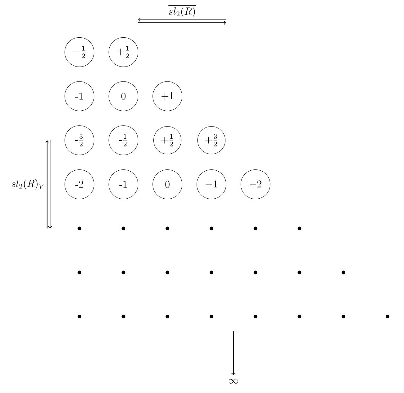
Figure 1: The figure shows the soft currents. The rows and the columns are indexed by the $\overline{sl_{2}(R)}$ weights and the dimension $(\Delta=k=1,0,-1,-2,...)$ of the conformally soft graviton $H^{k}(z,\bar{z})$, which generates the currents sitting in a row, respectively. $\overline{sl_{2}(R)}$ acts horizontally along a row and $sl_{2}(R)_{V}$ acts vertically along a column. In this way they generate the whole symmetry algebra starting from the current $H^{1}_{\frac{1}{2}}(z)$ on the top left corner.

Now let us consider the currents $\{H^{1}_{\frac{1}{2}},H^{0}_{1},...,H^{k}_{\frac{2-k}{2}},...\}$ with the lowest $\overline{sl_{2}(R)}$ weights. These currents transform in an irreducible highest weight representation of the $sl_{2}(R)_{V}$. This can be seen from the following commutation relations following from (5),

$$\begin{gathered}\left[H^{-1}_{\frac{1}{2},\frac{1}{2}},H^{k}_{\alpha,\frac{2-k}{2}}\right]=-\frac{1}{2}(k-2)(k-3)H^{k-1}_{\alpha+\frac{1}{2},\frac{2-(k-1)}{2}}\\ \left[H^{0}_{0,0},H^{k}_{\alpha,\frac{2-k}{2}}\right]=(k-2)H^{k}_{\alpha,\frac{2-k}{2}}\\ \left[H^{1}_{-\frac{1}{2},-\frac{1}{2}},H^{k}_{\frac{2-k}{2}}\right]=-H^{k+1}_{\alpha-\frac{1}{2},\frac{2-(k+1)}{2}}\end{gathered}$$ (26)

Therefore, starting from the current $H^{1}_{\frac{1}{2}}(z)$ we can generate any other $w$ current by the combined action of the $\overline{sl_{2}(R)}$ and $sl_{2}(R)_{V}$ (Fig.1).

Now, the way it is reflected in the structure of the OPE is the following. Suppose we consider the OPE of two positive helicity gravitons. The OPE is $w$ invariant if the singular terms have the following universal structure

$$G^{+}_{\Delta_{1}}(z,\bar{z})G^{+}_{\Delta_{2}}(0,0)\supset-\frac{\bar{z}}{z}\sum_{n=0}^{\infty}B\left(\Delta_{1}-1+n,\Delta_{2}-1\right)\frac{{\bar{z}}^{n}}{n!}\bar{\partial}^{n}G^{+}_{\Delta_{1}+\Delta_{2}}(0,0)$$ (27)

Now it has been shown in Pate:2019lpp that the leading term in $\bar{z}$ is uniquely determined by the $sl_{2}(R)_{V}$ invariance. Once we know the leading term, the subleading terms in $\bar{z}$ of $\mathcal{O}(\frac{\bar{z}^{q}}{z}),q\geq 2$ are determined by the $\overline{sl_{2}(R)}$ invariance. Therefore if we make sure that the $sl_{2}(R)_{V}$ and the $\overline{sl_{2}(R)}$ symmetries are not broken then we are bound to have $w$ invariance. We now discuss the consequences of this.

V.1 $w$ invariance at $\mathcal{O}(z^{0}\bar{z}^{0})$

In section-(IV) we have shown that the equations

$$\Omega_{k+1}(\Delta)=0,\ k\geq n\geq 0$$ (28)

are $sl_{2}(R)_{V}$ invariant. Now one can easily check that

$$H^{0}_{0,1}\Omega_{k}(\Delta)=0$$ (29)

where $H^{0}_{0,1}$ is, upto normalization, $\bar{L}_{1}$. So the MHV null states $\Omega_{k}(\Delta)$ are $\overline{sl_{2}(R)}$ primaries and as a result the equations (28) are $\overline{sl_{2}(R)}$ invariant. This implies that (28) is also $w$ invariant.

For the same reason, the additional null state relations (22)

$$\chi^{i}_{n}(\Delta)=0,\ i=1,2,...,\lceil{\frac{n}{2}}\rceil$$ (30)

at $\mathcal{O}(z^{0}\bar{z}^{0})$ are also $w$ invariant.

V.2 $w$ invariance at $\mathcal{O}(z^{0}\bar{z}^{1})$

Similarly, we have shown in section-(IV) that the equations

$$\Pi_{k+1}(\Delta)=0,\ k\geq n^{\prime}\geq 0$$ (31)

are $sl_{2}(R)_{V}$ invariant. Now the action of $H^{0}_{0,1}$ on $\Pi_{k}(\Delta)$ is given by,

$$\begin{gathered}H^{0}_{0,1}\Pi_{k+1}(\Delta)=-(\Delta+k-2)\Omega_{k+1}(\Delta-1)+(k+3)\Omega_{k+2}(\Delta-1)\end{gathered}$$ (32)

So if we want to impose (31) without breaking the $\overline{sl_{2}(R)}$ invariance then we also have to impose

$$\Omega_{k+1}(\Delta)=0,\ k\geq n^{\prime}\geq 0$$ (33)

Therefore, (31) is $w$ invariant if (33) holds and we know from our previous analysis that (33) is indeed $w$ invariant. This also shows that $n_{0,0}=n_{0,1}$ in (10) as a consequence of $w$ invariance.

VI Finiteness and an infinite family of theories

Our analysis in the last section shows that $w$ symmetry remains unbroken if we set

$$\Omega_{k+1}(\Delta)=0,\ k\geq n\geq 0$$ (34)

and

$$\Pi_{k+1}(\Delta)=0,\ k\geq n\geq 0$$ (35)

simultaneously. Therefore we can construct a $w$ invariant OPE at $\mathcal{O}(z^{0}\bar{z}^{0})$ and $\mathcal{O}(z^{0}\bar{z}^{1})$ by keeping only the finite number of MHV null states $\{\Omega_{1}(\Delta),...,\Omega_{n}(\Delta)\}$ and $\{\Pi_{1}(\Delta),\cdots,\Pi_{n}(\Delta)\}$, respectively. The crucial point here is that the value of the integer n, is not fixed by $w$ invariance. So we get different $w$ invariant OPEs for different choices of the integer $n$. For example, $n=0$ gives the MHV-sector. Similarly, direct calculation of graviton-graviton OPE using the scattering amplitudes shows that $n=4$ gives the OPE of the quantum self-dual gravity theory which is known to be $w$ invariant Ball:2021tmb . The existence of this discrete infinite family of $w$ invariant OPEs is the main outcome of our analysis.

VII $w$ invariant OPE coefficients

In this section we write down the $w$ invariant OPE for a given value of $n$, at $\mathcal{O}(z^{0}\bar{z}^{0})$ and $\mathcal{O}(z^{0}\bar{z}^{1})$, using the states $\{\Omega_{1}(\Delta),...,\Omega_{n}(\Delta)\}$ and $\{\Pi_{1}(\Delta),\cdots,\Pi_{n}(\Delta)\}$. At $\mathcal{O}(z^{0}\bar{z}^{0})$ we have

$$\begin{gathered}G^{+}_{\Delta_{1}}(z,\bar{z})G^{+}_{\Delta_{2}}(0,0)\big{|}_{\mathcal{O}(z^{0}\bar{z}^{0})}=G^{+}_{\Delta_{1}}(z,\bar{z})G^{+}_{\Delta_{2}}(0,0)\big{|}_{\text{MHV at}\ \mathcal{O}(z^{0}\bar{z}^{0})}\\ +\sum_{p=1}^{n}B(\Delta_{1}-1+p,\Delta_{2}-1)\ \Omega_{p}(\Delta_{1}+\Delta_{2})\end{gathered}$$ (36)

and at $\mathcal{O}(z^{0}\bar{z}^{1})$

$$\begin{gathered}G^{+}_{\Delta_{1}}(z,\bar{z})G^{+}_{\Delta_{2}}(0,0)\big{|}_{\mathcal{O}(z^{0}\bar{z}^{1})}=G^{+}_{\Delta_{1}}(z,\bar{z})G^{+}_{\Delta_{2}}(0,0)\big{|}_{\text{MHV at}\ \mathcal{O}(z^{0}\bar{z}^{1})}\\ +\bar{z}\sum_{p=1}^{n}B(\Delta_{1}+p,\Delta_{2}-1)\ \Pi_{p}(\Delta_{1}+\Delta_{2}+1)\end{gathered}$$ (37)

The MHV sector OPE at $\mathcal{O}(z^{0}\bar{z}^{0})$ and $\mathcal{O}(z^{0}\bar{z}^{1})$ are given in Banerjee:2020zlg .

As we have already discussed the states $\{\Omega_{1}(\Delta),...,\Omega_{n}(\Delta)\}$ are not all independent because of the existence of the additional null state relations (22)

$$\chi^{i}_{n}(\Delta)=0,\ i=1,2,...,\lceil{\frac{n}{2}}\rceil$$ (38)

We can further simplify (36) by using these null state relations. However, we choose to leave it in this form because the OPE coefficients are particularly nice when written in terms of these linearly dependent states. Now different values of $n$ give OPEs in different $w$ invariant theories. We now discuss the KZ type null states of these theories.

VIII Knizhnik-Zamolodchikov type null states

KZ type null states occur at $\mathcal{O}(z^{0}\bar{z}^{1})$ of the OPE. The simplest way to derive it is to demand the commutativity of the OPE, i.e,

$$G^{+}_{\Delta_{1}}(z_{1},\bar{z}_{1})G^{+}_{\Delta_{2}}(z_{2},\bar{z}_{2})=G^{+}_{\Delta_{2}}(z_{2},\bar{z}_{2})G^{+}_{\Delta_{1}}(z_{1},\bar{z}_{1})$$ (39)

If we use the consistency condition (39) and the OPE given in (36) and (37) we get the following KZ type null state

$$\boxed{\Xi_{n}(\Delta)=\xi(\Delta)+\sum_{k=1}^{n}\Pi_{k}(\Delta+1)=0}$$ (40)

where $\xi(\Delta)$ is the KZ type null state in the MHV sector given by Banerjee:2020zlg

$$\xi(\Delta)=\boxed{L_{-1}}G^{+}_{\Delta}+H^{0}_{0,-1}H^{1}_{-\frac{3}{2},\frac{1}{2}}G^{+}_{\Delta-1}+H^{0}_{-1,0}G^{+}_{\Delta}+(\Delta-1)\,H^{1}_{-\frac{3}{2},-\frac{1}{2}}G^{+}_{\Delta-1}$$ (41)

We have used that $\chi^{1}_{n}(\Delta)$ is a null state in this theory to arrive at the form (40).

As consistency checks we can compute the actions of $\overline{sl_{2}(R)}$ and $sl_{2}(R)_{V}$ generators on $\Xi_{n}(\Delta)$. For example,

$$H^{0}_{0,1}\Xi_{n}(\Delta)=(n+2)\Omega_{n+1}(\Delta)-(\Delta-3)\chi^{1}_{n}(\Delta)=0$$ (42)

because $\Omega_{n+1}(\Delta)$ and $\chi^{1}_{n}(\Delta)$ are both null states in this theory. Therefore $\Xi_{n}(\Delta)$ is a $\overline{sl_{2}(R)}$ primary.

Similarly, we have

$$\begin{gathered}H^{-1}_{\frac{1}{2},\frac{1}{2}}\Xi_{n}(\Delta)=-\frac{1}{2}(\Delta-2)(\Delta-3)\Xi_{n}(\Delta-1)\\ -\frac{1}{2}(n+2)(n-1)\Pi_{n+1}(\Delta)-H^{-1}_{\frac{1}{2},-\frac{1}{2}}\chi^{1}_{n}(\Delta)-H^{0}_{0,-1}\left((\Delta-1)\chi^{1}_{n}(\Delta-1)+\chi^{2}_{n}(\Delta-1)\right)\\ \end{gathered}$$ (43)

But, since $\Pi_{n+1}(\Delta),\chi^{1}_{n}(\Delta)$ and $\chi^{2}_{n}(\Delta)$ are null states in the theory, we get

$$H^{-1}_{\frac{1}{2},\frac{1}{2}}\Xi_{n}(\Delta)=-\frac{1}{2}(\Delta-2)(\Delta-3)\Xi_{n}(\Delta-1)$$ (44)

Therefore $\Xi_{n}(\Delta)$ transforms under a representation of the $sl_{2}(R)_{V}$ and we can consistently set it to zero without violating the $sl_{2}(R)_{V}$ symmetry. Therefore, (40) is indeed $w$ invariant.

Decoupling of null states gives rise to differential equations which the graviton scattering amplitudes in this theory have to satisfy. So in principle we know a lot about these theories however, solving these equations may not be easy in practice. We hope to return to this in near future.

IX Acknowledgements

We would like to thank Andrew Strominger and Sabrina Pasterski for useful discussion. The work of SB is partially supported by the Swarnajayanti Fellowship (File No- SB/SJF/2021-22/14) of the Department of Science and Technology and SERB, India and by SERB grant MTR/2019/000937 (Soft-Theorems, S-matrix and Flat-Space Holography). The work of HK is partially supported by the KVPY fellowship of the Department of Science and Technology (DST), Government of India and the Summer Students’ Visiting Program at the Institute of Physics, Bhubaneswar, India. The work of PP is supported by an IOE endowed postdoctoral position at IISc, Bengaluru, India.

References

- (1) A. Strominger, “Lectures on the Infrared Structure of Gravity and Gauge Theory,” [arXiv:1703.05448 [hep-th]]. A. M. Raclariu, “Lectures on Celestial Holography,” [arXiv:2107.02075 [hep-th]]. S. Pasterski, “Lectures on celestial amplitudes,” Eur. Phys. J. C 81, no.12, 1062 (2021) doi:10.1140/epjc/s10052-021-09846-7 [arXiv:2108.04801 [hep-th]] S. Pasterski, M. Pate and A. M. Raclariu, “Celestial Holography,” [arXiv:2111.11392 [hep-th]].
- (2) S. Pasterski, S. H. Shao and A. Strominger, “Flat Space Amplitudes and Conformal Symmetry of the Celestial Sphere,” Phys. Rev. D 96, no. 6, 065026 (2017) doi:10.1103/PhysRevD.96.065026 [arXiv:1701.00049 [hep-th]].
- (3) S. Pasterski and S. H. Shao, “Conformal basis for flat space amplitudes,” Phys. Rev. D 96, no. 6, 065022 (2017) doi:10.1103/PhysRevD.96.065022 [arXiv:1705.01027 [hep-th]].
- (4) S. Banerjee, “Null Infinity and Unitary Representation of The Poincare Group,” JHEP 1901, 205 (2019) doi:10.1007/JHEP01(2019)205 [arXiv:1801.10171 [hep-th]].
- (5) R. Sachs, “Asymptotic symmetries in gravitational theory,” Phys. Rev. 128, 2851 (1962). doi:10.1103/PhysRev.128.2851 H. Bondi, M. G. J. van der Burg and A. W. K. Metzner, “Gravitational waves in general relativity. 7. Waves from axisymmetric isolated systems,” Proc. Roy. Soc. Lond. A 269, 21 (1962). doi:10.1098/rspa.1962.0161 R. K. Sachs, “Gravitational waves in general relativity. 8. Waves in asymptotically flat space-times,” Proc. Roy. Soc. Lond. A 270, 103 (1962). doi:10.1098/rspa.1962.0206
- (6) A. Strominger, “On BMS Invariance of Gravitational Scattering,” JHEP 1407, 152 (2014) doi:10.1007/JHEP07(2014)152 [arXiv:1312.2229 [hep-th]].
- (7) T. He, V. Lysov, P. Mitra and A. Strominger, “BMS supertranslations and Weinberg’s soft graviton theorem,” JHEP 1505, 151 (2015) doi:10.1007/JHEP05(2015)151 [arXiv:1401.7026 [hep-th]]. A. Strominger and A. Zhiboedov, “Gravitational Memory, BMS Supertranslations and Soft Theorems,” JHEP 1601, 086 (2016) doi:10.1007/JHEP01(2016)086 [arXiv:1411.5745 [hep-th]].
- (8) G. Barnich and C. Troessaert, “Symmetries of asymptotically flat 4 dimensional spacetimes at null infinity revisited,” Phys. Rev. Lett. 105, 111103 (2010) doi:10.1103/PhysRevLett.105.111103 [arXiv:0909.2617 [gr-qc]].
- (9) G. Barnich and C. Troessaert, “Supertranslations call for superrotations,” PoS CNCFG 2010, 010 (2010) [Ann. U. Craiova Phys. 21, S11 (2011)] [arXiv:1102.4632 [gr-qc]].
- (10) D. Kapec, P. Mitra, A. M. Raclariu and A. Strominger, “2D Stress Tensor for 4D Gravity,” Phys. Rev. Lett. 119, no. 12, 121601 (2017) doi:10.1103/PhysRevLett.119.121601 [arXiv:1609.00282 [hep-th]].
- (11) D. Kapec, V. Lysov, S. Pasterski and A. Strominger, “Semiclassical Virasoro symmetry of the quantum gravity -matrix,” JHEP 1408, 058 (2014) doi:10.1007/JHEP08(2014)058 [arXiv:1406.3312 [hep-th]].
- (12) T. He, D. Kapec, A. M. Raclariu and A. Strominger, “Loop-Corrected Virasoro Symmetry of 4D Quantum Gravity,” JHEP 1708, 050 (2017) doi:10.1007/JHEP08(2017)050 [arXiv:1701.00496 [hep-th]].
- (13) L. Donnay, S. Pasterski and A. Puhm, “Asymptotic Symmetries and Celestial CFT,” [arXiv:2005.08990 [hep-th]].
- (14) S. Stieberger and T. R. Taylor, “Symmetries of Celestial Amplitudes,” Phys. Lett. B 793, 141 (2019) doi:10.1016/j.physletb.2019.03.063 [arXiv:1812.01080 [hep-th]].
- (15) S. Banerjee and S. Pasterski, “Revisiting the Shadow Stress Tensor in Celestial CFT,” [arXiv:2212.00257 [hep-th]].
- (16) S. Banerjee, S. Ghosh and P. Paul, “MHV Graviton Scattering Amplitudes and Current Algebra on the Celestial Sphere,” [arXiv:2008.04330 [hep-th]].
- (17) S. Banerjee, S. Ghosh and S. Satyam Samal, “Subsubleading soft graviton symmetry and MHV graviton scattering amplitudes,” [arXiv:2104.02546 [hep-th]].
- (18) N. Gupta, P. Paul and N. V. Suryanarayana, “An Symmetry of Gravity,” [arXiv:2109.06857 [hep-th]]
- (19) A. Guevara, E. Himwich, M. Pate and A. Strominger, “Holographic Symmetry Algebras for Gauge Theory and Gravity,” [arXiv:2103.03961 [hep-th]].
- (20) A. Strominger, “w(1+infinity) and the Celestial Sphere,” [arXiv:2105.14346 [hep-th]]. A. Strominger, “ Algebra and the Celestial Sphere: Infinite Towers of Soft Graviton, Photon, and Gluon Symmetries,” Phys. Rev. Lett. 127, no.22, 221601 (2021) doi:10.1103/PhysRevLett.127.221601
- (21) E. Himwich, M. Pate and K. Singh, “Celestial operator product expansions and w1+∞ symmetry for all spins,” JHEP 01, 080 (2022) doi:10.1007/JHEP01(2022)080 [arXiv:2108.07763 [hep-th]].
- (22) A. Ball, S. A. Narayanan, J. Salzer and A. Strominger, “Perturbatively exact w1+∞ asymptotic symmetry of quantum self-dual gravity,” JHEP 01, 114 (2022) doi:10.1007/JHEP01(2022)114 [arXiv:2111.10392 [hep-th]].
- (23) L. Freidel, D. Pranzetti and A. M. Raclariu, “Sub-subleading soft graviton theorem from asymptotic Einstein’s equations,” JHEP 05, 186 (2022) doi:10.1007/JHEP05(2022)186 [arXiv:2111.15607 [hep-th]]
- (24) L. Freidel, D. Pranzetti and A. M. Raclariu, “Higher spin dynamics in gravity and w1+ celestial symmetries,” Phys. Rev. D 106, no.8, 086013 (2022) doi:10.1103/PhysRevD.106.086013 [arXiv:2112.15573 [hep-th]]
- (25) T. Adamo, L. Mason and A. Sharma, “Celestial Symmetries from Twistor Space,” SIGMA 18, 016 (2022) doi:10.3842/SIGMA.2022.016 [arXiv:2110.06066 [hep-th]].
- (26) K. Costello and N. M. Paquette, “Celestial holography meets twisted holography: 4d amplitudes from chiral correlators,” JHEP 10, 193 (2022) doi:10.1007/JHEP10(2022)193 [arXiv:2201.02595 [hep-th]].
- (27) S. Banerjee and S. Ghosh, “MHV Gluon Scattering Amplitudes from Celestial Current Algebras,” [arXiv:2011.00017 [hep-th]]. Y. Hu, L. Ren, A. Y. Srikant and A. Volovich, “Celestial dual superconformal symmetry, MHV amplitudes and differential equations,” JHEP 12, 171 (2021) doi:10.1007/JHEP12(2021)171 [arXiv:2106.16111 [hep-th]]. W. Fan, A. Fotopoulos, S. Stieberger, T. R. Taylor and B. Zhu, “Elements of celestial conformal field theory,” JHEP 08, 213 (2022) doi:10.1007/JHEP08(2022)213 [arXiv:2202.08288 [hep-th]]. W. Fan, A. Fotopoulos, S. Stieberger, T. R. Taylor and B. Zhu, “Celestial Yang-Mills amplitudes and D = 4 conformal blocks,” JHEP 09, 182 (2022) doi:10.1007/JHEP09(2022)182 [arXiv:2206.08979 [hep-th]]. Y. Hu and S. Pasterski, “Celestial Recursion,” [arXiv:2208.11635 [hep-th]]
- (28) M. Pate, A. M. Raclariu, A. Strominger and E. Y. Yuan, “Celestial Operator Products of Gluons and Gravitons,” arXiv:1910.07424 [hep-th].
- (29) A. Atanasov, W. Melton, A. M. Raclariu and A. Strominger, “Conformal Block Expansion in Celestial CFT,” [arXiv:2104.13432 [hep-th]].
- (30) S. Ghosh, P. Raman and A. Sinha, “Celestial insights into the S-matrix bootstrap,” JHEP 08, 216 (2022) doi:10.1007/JHEP08(2022)216 [arXiv:2204.07617 [hep-th]]
- (31) L. Donnay, A. Puhm and A. Strominger, “Conformally Soft Photons and Gravitons,” JHEP 1901, 184 (2019) doi:10.1007/JHEP01(2019)184 [arXiv:1810.05219 [hep-th]]. M. Pate, A. M. Raclariu and A. Strominger, “Conformally Soft Theorem in Gauge Theory,” arXiv:1904.10831 [hep-th]. W. Fan, A. Fotopoulos and T. R. Taylor, “Soft Limits of Yang-Mills Amplitudes and Conformal Correlators,” JHEP 1905, 121 (2019) doi:10.1007/JHEP05(2019)121 [arXiv:1903.01676 [hep-th]]. D. Nandan, A. Schreiber, A. Volovich and M. Zlotnikov, “Celestial Amplitudes: Conformal Partial Waves and Soft Limits,” arXiv:1904.10940 [hep-th]. T. Adamo, L. Mason and A. Sharma, “Celestial amplitudes and conformal soft theorems,” arXiv:1905.09224 [hep-th]. A. Puhm, “Conformally Soft Theorem In Gravity,” arXiv:1905.09799 [hep-th]. A. Guevara, “Notes on Conformal Soft Theorems and Recursion Relations in Gravity,” arXiv:1906.07810 [hep-th].