Accurate and efficient multiscale simulation of a heterogeneous elastic beam via computation on small sparse patches

Abstract

Modern ‘smart’ materials have complex microscale structure, often with unknown macroscale closure. The Equation-Free Patch Scheme empowers us to non-intrusively, efficiently, and accurately simulate over large scales through computations on only small well-separated patches of the microscale system. Here the microscale system is a solid beam of random heterogeneous elasticity. The continuing challenge is to compute the given physics on just the microscale patches, and couple the patches across un-simulated macroscale space, in order to establish efficiency, accuracy, consistency, and stability on the macroscale. Dynamical systems theory supports the scheme. This research program is to develop a systematic non-intrusive approach, both computationally and analytically proven, to model and compute accurately macroscale system levels of general complex physical and engineering systems.

1 Introduction

In structural engineering, microscale lattice materials can be light and highly stiff with customizable macroscale mechanical properties (e.g., Somnic & Jo 2022). The challenge we address herein is to accurately and efficiently predict macroscale characteristics emergent from the microscale lattice. Similarly, composite materials and structures are inherently heterogeneous and anisotropic across multiple scales. Multiscale modelling is thus critical to the design of composite structures for lightweight mechanical performance (e.g., Raju et al. 2021, Lucarini et al. 2021). Such composite materials are used in electronics, space, medical, transportation, and other industries (e.g. Matouš et al. 2017). Herein we establish that the Equation-Free Patch Scheme can non-intrusively, efficiently, and accurately simulate over macroscales through computations on only small well-separated patches of the microscale system.

Figure 1: movie of a full-domain simulation of a heterogeneous beam showing that beam bending waves and longitudinal compression waves propagate with some ‘average’ properties.

[controls,width=every=3]10Figs/beamFullLong/i1301

Consider an example elastic beam with heterogeneous elasticity in 2D as in fig. 1: say 628 cm long, 20 cm wide. The beam is heterogeneous because it is constructed from a modern material with micro-structure of size 3 cm—so that the heterogeneity is ‘visible’ in fig. 1. With a 3 cm micro-grid, the modelling requires circa 5 000 variables. This specific scenario is easily computable, ode23 took 14 s cpu time to simulate one period of beam bending oscillation. But if a more realistic 3 mm micro-structure is simulated, then the computation time increases by a factor of 1000. If 3D elasticity modelling is required for the beam, then the computation time increases by even more orders of magnitude. The patch scheme (e.g., Samaey et al. 2010) we develop herein potentially reduces macroscale computation time by orders of magnitude—more reduction in higher-D space and/or smaller micro-scale.

The patch scheme achieves efficiency by only computing on small sparse patches in space. section 2.1 discusses how the patch scheme is non-intrusive in that it just ‘wraps around’ a user’s microscale code—a desirable property also identified by Biezemans et al. (2022). The patch scheme, alternatively called the gap-tooth method, “has formal similarity with sp [superparametrization]” (Majda & Grooms 2014, p.62) that was developed in meteorology for weather and climate predictions, and is also akin to the so-called fe-fft and fe² methods (Lucarini et al. 2021, e.g.,§4.7).

A given microscale discretisation of heterogeneous elasticity

We adopt a simple robust microscale approximation of 2D elasticity within the beam. On the staggered microscale $xy$-grid of fig. 2 define the displacements: $\color[rgb]{0,0,1}\blacktriangleright$, horizontal $u_{ij}(t)$; $\color[rgb]{1,0,0}\blacktriangle$, vertical $v_{ij}(t)$.

Figure 2: a small part of the microscale grid used to code 2D elasticity. The grid is staggered on the microscale: $\color[rgb]{0,0,1}\blacktriangleright$, horizontal displacements and velocities; $\color[rgb]{1,0,0}\blacktriangle$, vertical displacements and velocities; $\color[rgb]{0,0.7,0}\circledcirc$, $\color[rgb]{0,0.7,0}\otimes$, components of strain and stress tensor (1).

Microscale elasticity here first uses centred finite differences to compute stresses, for heterogeneous Lamé parameters $\lambda,\mu$, at the labelled microscale grid-points (fig. 2):

$$\text{$\color[rgb]{0,0.7,0}\otimes$}\quad\sigma_{xy}:=\mu_{ij}\big{[}\delta_{j}u_{ij}/\delta y_{j}+\delta_{i}v_{ij}/\delta x_{i}\big{]};$$ (1a)

$$\text{$\color[rgb]{0,0.7,0}\circledcirc$}\quad\sigma_{xx}:=(\lambda_{ij}+2\mu_{ij}){\delta_{i}u_{ij}}/{\delta x_{i}}+\lambda_{ij}{\delta_{j}v_{ij}}/{\delta y_{j}};$$ (1b)

$$\text{$\color[rgb]{0,0.7,0}\circledcirc$}\quad\sigma_{yy}:=\lambda_{ij}{\delta_{i}u_{ij}}/{\delta x_{i}}+(\lambda_{ij}+2\mu_{ij}){\delta_{j}v_{ij}}/{\delta y_{j}}.$$ (1c)

Second, centred finite differences compute the following acceleration odes

$$\text{$\color[rgb]{0,0,1}\blacktriangleright$}\quad\ddot{u}_{ij}={\delta_{i}\sigma_{xx}}/{\delta x_{i}}+{\delta_{j}\sigma_{xy}}/{\delta y_{j}}\,,$$ (2a)

$$\text{$\color[rgb]{1,0,0}\blacktriangle$}\quad\ddot{v}_{ij}={\delta_{i}\sigma_{xy}}/{\delta x_{i}}+{\delta_{j}\sigma_{yy}}/{\delta y_{j}}\,,$$ (2b)

potentially with optional small phenomenological damping supplied by a discretisation of $\kappa\nabla^{2}\dot{u}_{ij},\,\kappa\nabla^{2}\dot{v}_{ij}$. The patch scheme wraps around whatever microscale code a user supplies—here it is the microscale system (LABEL:eqs:stress,eqs:accel)

We nondimensionalise the system so that the density is one, and the speed of a macroscale compression wave along the beam is about one, that is, time in these simulations is roughly in milli-seconds.

Random periodic heterogeneity

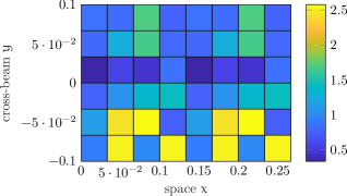
Figure 3: example of the 2D microscale heterogeneous Young’s modulus $E_{ij}$ used in computing the elastic Lamé parameters (3). In this example, we choose the heterogeneity to have microscale period four along the beam.

The Lamé parameters which appear in the stresses (1) are

$$\lambda:=\frac{\nu E}{(1+\nu)(1-2\nu)},\quad\mu:=\frac{E}{2(1+\nu)},$$ (3)

in terms of Young’s modulus $E$ and Poisson ratio $\nu$. To have strong microscale heterogeneity we choose these parameters randomly so that at each microscale grid-point (iid): $E_{ij}$ is log-normal (here varies by factor of about ten); and $\nu_{ij}$ is uniform on $[0.25,0.35]$. fig. 3 shows an example $E_{ij}$. Despite such strong heterogeneity, the movie of fig. 1 shows the macroscale dynamics appears relatively simple.

Figure 4: movie of a patch scheme simulation of a heterogeneous beam showing the macroscale propagation across the patches of beam bending waves and longitudinal compression waves.

[controls,width=every=3]10Figs/beamSim/i1301

2 Equation-free patch scheme

Instead of computing the entire beam as seen in fig. 1, the patch scheme computes only in small sparse spatial patches such as fig. 4. In this example case, the patch scheme reduces compute time by a factor${}\propto r:={}$(patch size)/(spacing $H$), which here is just a modest factor of $1/4$. But with greater scale separation and/or in higher spatial dimensions, the scheme often reduces computational time by many orders of magnitude.

The movie of fig. 4 shows a slow progressive wave of beam bending, together with a not-so-slow compression wave along the beam. These macroscale predictions are accurate (section 3) due to the correctness of our simple coupling between patches—even when heterogeneity is strong. The patch scheme makes these accurate macroscale predictions even when the macroscale closure is unknown: the scheme does not code a closure. Further, ‘the closure’ varies depending upon human assumptions such as choosing averaged models versus cosserat models—the patch scheme makes no such closure assumptions. The only assumption is that the macroscale quantities of importance vary smoothly between neighbouring patches.

2.1 Scheme is non-intrusive functional ‘wrapper’

Consider one of the patches of the 2D beam shown in fig. 4. With the given microscale $xy$-grid (fig. 2), zooming in to the microscale each patch is like that of fig. 5. Here each patch extends across the cross-section ($y$-dimension) of the beam. Open symbols in fig. 5 are ghost nodes outside the patch and implement given stress-free top/bottom conditions on the beam. The only addition required by the patch scheme are the edge values (‘squared’ micro-grid nodes in fig. 5) on the left/right of each patch.

Figure 5: one example patch of the 2D elastic beam showing the microscale staggered grid (fig. 2). This is case of $n_{\text{subpatch}}=7$ micro-grid intervals along the patch, and $n_{y}=4$ intervals across the beam.

The patch scheme couples patches together by providing the patch-edge values through interpolation across the macroscale between patches (e.g., Roberts & Kevrekidis 2007, Roberts et al. 2014, Cao & Roberts 2016). Here we interpolate from each of the centre patch values across the beam ($i=4$ in fig. 5) of ‘nearby’ patches, to determine the corresponding patch-edge value. Here we implement spectral (fft) interpolation between the patches for high accuracy (section 3). The scheme does not presume that any average is appropriate.

This implementation shows that the patch scheme is non-intrusive (e.g., Biezemans et al. 2022): it just ‘wraps around’ any micro-grid code a user trusts. Consequently, we provide a toolbox Maclean et al. (2021) for others to implement the patch scheme around their micro-code.

2.2 Scheme embeds macroscale dynamics

Given the patch scheme does not assume anything about what are ‘correct’ macroscale variables, a crucial question is the following: how can we be assured that the patch scheme captures the macroscale slow dynamics?  An answer is provided by the Whitney (1936) embedding theorem.

Roughly, the theorem is that every $m$D manifold is parametrisable from almost every subspace of more than $2m$D. Let’s see what this means for us. In essence, the patch scheme provides the higher-D subspace in which the slow manifold of the macroscale wave dynamics is embedded.

For beams in two spatial dimensions, the basic macroscale beam models have, at each cross-section, displacement and velocity of both bending and compression. Thus the elastic beam dynamics has a slow manifold that is $m=4$D at every cross-section. Alternatively, 2D cosserat beam models add a shear mode to the macroscale model—two more variables—leading to a not-quite-so-slow manifold of $m=6$D at every cross-section. These physically based models are slow manifolds because they focus on the relatively slow waves of solutions varying slowly in space, and neglect all the faster high-frequency cross-waves.

In the patch scheme, figs. 1 and 4 show simulations with a cross-section of $n_{y}=7$ micro-grid intervals, but let’s discuss the case of just $n_{y}=4$ (fig. 5). For $n_{y}=4$, there are seven microscale nodes across each patch edge. Each node has a displacement and velocity, and so leads to a $14$D subspace for macroscale communication between patches.

Because $14>2\cdot 6>2\cdot 4$ , the Whitney embedding theorem asserts that the patch scheme exchanges enough information to almost surely parametrise both such slow manifolds of the macroscale dynamics. The patch scheme does not need to explicitly compute and exchange specific assumed macroscale average quantities.

3 Scheme has proven accuracy

section 3.2 discusses established theory which generally proves that the patch scheme makes accurate macroscale predictions. Such proofs are in stark contrast to the vast machine learning/artificial intelligence developments which prove very few general results: for example, Brenner & Koumoutsakos (2021) comment “…ml studies, as the lack of rigorous theory does not offer (yet!) guarantees of convergence”. Before discussing theory, we first report some computational verification of high accuracy.

3.1 Computation verifies exactness

Figure 6: multiscale spectrum of eigenvalues $\lambda$ separates macroscale modes on the right from sub-patch microscale modes on the left. The axes are scaled nonlinearly. Here the small viscosity is $0.001$ so the microscale decays, but the macroscale waves are long-lasting.

Here we restricted attention to linear elasticity so we know that the wrapped patch system is fully characterised by the resultant Jacobian matrix. We numerically compute the Jacobian matrix of the patch scheme by elementary numerical differentiation.

Because of the macroscale translational invariance of the patch scheme, the macroscale eigenvectors are correctly sinusoidal. Hence the only macroscale errors occur in the eigenvalues of the Jacobian. fig. 6 plots the spectrum of all eigenvalues for one example of random heterogeneity, in the case of five patches for simplicity. Observe there are:

• (on the right) four $\lambda=0$ of rigid beam motion;

• four $-0.001\pm\operatorname{i}1.057$ and four $-0.003\pm\operatorname{i}2.111$ of compressions waves;

• four $-0.001\pm\operatorname{i}0.061$ and four $-0.004\pm\operatorname{i}0.237$ of beam bending waves;

• with the above macroscale eigenvalues separated by a spectral gap from the following sub-patch microscale eigenvalues;

• (on the left) many $\Re\lambda<-0.1$ of uninteresting sub-patch micro-scale fast-waves (headed by ten eigenvalues around $-0.14\pm\operatorname{i}9.29$).

To quantify the accuracy, table 1 compares eigenvalues obtained from full-domain code, with the above macroscale eigenvalues obtained by the wrapped patch scheme. For all patch size ratios and heterogeneities tested, the patch scheme’s macroscale eigenvalues are exact to numerical round-off error.

Table 1: error in patch scheme’s macroscale eigenvalues $\lambda$ for various patch size ratios $r$: the macroscale $\lambda$s are exact to round-off error—due to patch coupling by spectral interpolation.

macro-eigenvalue	$r=\tfrac{1}{2}$	$r=\tfrac{1}{4}$	$r=\tfrac{1}{8}$
$-0.001\pm\operatorname{i}0.061$	2e-12	1e-12	2e-13
$-0.001\pm\operatorname{i}0.061$	2e-12	4e-12	2e-12
$-0.004\pm\operatorname{i}0.237$	1e-12	8e-13	3e-12
$-0.004\pm\operatorname{i}0.237$	1e-12	2e-12	3e-12
$-0.001\pm\operatorname{i}1.057$	7e-13	4e-13	6e-13
$-0.001\pm\operatorname{i}1.057$	6e-13	5e-13	6e-13
$-0.003\pm\operatorname{i}2.111$	1e-13	2e-13	2e-13
$-0.003\pm\operatorname{i}2.111$	4e-13	5e-13	2e-13

Such exactness is due to the spectral interpolation used here. If, instead of spectral, local polynomial interpolation of degree $p$ is used to couple the patches, then generally the patch scheme has macroscale errors${}\propto H^{p}$ where $H={}$inter-patch spacing (e.g., Roberts & Kevrekidis 2007, Roberts et al. 2014).

Figure 7: multiscale spectrum of eigenvalues $\lambda$ for the patch scheme in the case of zero viscosity. The horizontal axis shows that all modes have zero real-part to numerical round-off error. That is, in the case of zero viscosity, this patch scheme preserves the wave nature of the underlying physics.

Undamped waves?

With zero viscosity, there are only oscillations in the underlying physics. In such a scenario computational methods are very delicate. Here, fig. 7 illustrates that all eigenvalues of the patch scheme have $|\Re\lambda|<10^{-12}$. Hence, even with no viscosity, the patch scheme preserves the oscillatory wave nature of the heterogeneous physics.

There is a perception that the patch scheme “only works well on problems with an inertial manifold and for systems in which most modes are strongly decaying” (Majda & Grooms 2014, p.62). This verification of accuracy for purely elastic beams shows that this perception is false. Applications and theory for other wave systems also refute this perception (e.g., Cao & Roberts 2016, Bunder et al. 2021, Divahar et al. 2022).

3.2 Mathematical analysis proves consistency

Mathematical analysis has proven properties of the patch scheme in general. Mostly, the published proofs explicitly address dissipative (nonlinear) systems. However, as discussed by Bunder et al. (2021), the patch scheme in space only recasts spatial interactions, so whether the time derivative is $\mathchoice{\frac{\partial}{\partial t}}{{\partial}/{\partial t}}{{\partial}/{\partial t}}{{\partial}/{\partial t}}$ of dissipation or $\mathchoice{\frac{\partial^{2}}{\partial t^{2}}}{{\partial^{2}}/{\partial t^{2}}}{{\partial^{2}}/{\partial t^{2}}}{{\partial^{2}}/{\partial t^{2}}}$ of waves makes little difference.

Two complementary types of results have been proven. They involve the spacing between patch centres $H$. First, Centre Manifold Theory may be applied at finite spacing $H$ by introducing a ‘bookkeeping’ parameter $\gamma$ to label inter-patch communication (e.g., Roberts et al. 2014, §2) to prove the existence of a slow manifold in the patch scheme (including when it is applied to nonlinear systems). Then the parameter $\gamma$ structures inter-patch interactions, and their algebraic expression, to empower theory based at $\gamma=0$, via regular perturbation, to address finite $\gamma$ such as the case of full coupling $\gamma=1$ (e.g., Roberts et al. 2014, Cor. 2).

Second, the patch scheme is consistent with the underlying micro-code as the patch spacing $H\to 0$ (e.g., Roberts et al. 2014, Thm. 7). The consistency is that the macroscale of the patch scheme is the same as the macroscale of the given micro-coded system, to errors $\mathcal{O}\mathchoice{\big{(}H^{p}\big{)}}{\big{(}H^{p}\big{)}}{(H^{p})}{(H^{p})}$ when using polynomial interpolation of degree $p$. For example, spectral interpolation corresponds to ‘$p=\infty$’ so then errors vanish to all orders as in table 1.

These results and general proofs were first done for homogeneous systems (e.g., Roberts & Kevrekidis 2007, Roberts et al. 2014). They were subsequently extended to heterogeneous microscales Bunder et al. (2017), and recently extended to alternative inter-patch coupling that preserves self-adjointness Bunder et al. (2021). Interestingly, the extension of the theoretical support to heterogeneous cases invokes the ensemble of all phase-shifts of the heterogeneity. The ensemble is spatially homogeneous, so the homogeneous proofs and results apply to establish the heterogeneous results.

4 Conclusion

As an initial exploration of the patch scheme for homogenisation of heterogeneous elasticity, we considered the prototypical case of a 2D elastic beam. The scheme gives a non-intrusive and efficient computational homogenisation of given microscale system via spatially sparse small patches. The patch coupling has proven accuracy, controllable error, at finite scale separation.

The patch scheme makes only one assumption: in the scenarios of interest to a user, there is no significant spatial structures in the mesoscale between the patch spacing $H$ and the microscale resolved in the patches. In contrast to most other multiscale methods, there is: no assumed boundary conditions on Representative Volume Elements (variously periodic, Dirichlet, Neumann); no explicitly assuming slow variables; and no presumed necessary variational principle. The scheme is entirely physically interpretable: there is no hidden mystic machinations of neural networks (e.g., Brenner & Koumoutsakos 2021)

The patch scheme is simple to apply. In contrast to other multiscale methods there is: no arbitrary averaging; no oversampling regions; no buffer regions; no action regions; no guessed fast/slow variables; no epsilons; and no limits. As a non-intrusive ‘wrapper’, anyone can start using the patch scheme via a Matlab/Octave Toolbox Maclean et al. (2021), Roberts et al. (2019–2024)

Acknowledgements

This research was supported by Australian Research Council grants DP220103156 and DP200103097.

References

- (1)
- Biezemans et al. (2022) Biezemans, R. A., Le Bris, C., Legoll, F. & Lozinski, A. (2022), Non-intrusive implementation of a wide variety of Multiscale Finite Element Methods, Technical report, http://arxiv.org/abs/2211.17024.
- Brenner & Koumoutsakos (2021) Brenner, M. P. & Koumoutsakos, P. (2021), ‘Editorial: Machine Learning and Physical Review Fluids: An Editorial Perspective’, Physical Review Fluids 6(7), 070001.
- Bunder et al. (2021) Bunder, J. E., Kevrekidis, I. G. & Roberts, A. J. (2021), ‘Equation-free patch scheme for efficient computational homogenisation via self-adjoint coupling’, Numerische Mathematik 149(2), 229–272.
- Bunder et al. (2017) Bunder, J. E., Roberts, A. J. & Kevrekidis, I. G. (2017), ‘Good coupling for the multiscale patch scheme on systems with microscale heterogeneity’, J. Computational Physics 337, 154–174.
- Cao & Roberts (2016) Cao, M. & Roberts, A. J. (2016), ‘Multiscale modelling couples patches of nonlinear wave-like simulations’, IMA J. Applied Maths. 81(2), 228–254.
- Divahar et al. (2022) Divahar, J., Roberts, A. J., Mattner, T. W., Bunder, J. E. & Kevrekidis, I. G. (2022), Two novel families of multiscale staggered patch schemes efficiently simulate large-scale, weakly damped, linear waves, Technical report, https://arxiv.org/abs/2210.15823.
- Lucarini et al. (2021) Lucarini, S., Upadhyay, M. V. & Segurado, J. (2021), ‘FFT based approaches in micromechanics: fundamentals, methods and applications’, Modelling and Simulation in Materials Science and Engineering 30(2), 023002.
- Maclean et al. (2021) Maclean, J., Bunder, J. E. & Roberts, A. J. (2021), ‘A toolbox of equation-free functions in matlab/octave for efficient system level simulation’, Numerical Algorithms 87, 1729–1748.
- Majda & Grooms (2014) Majda, A. J. & Grooms, I. (2014), ‘New perspectives on superparameterization for geophysical turbulence’, Journal of Computational Physics 271, 60–77.
- Matouš et al. (2017) Matouš, K., Geers, M. G. D., Kouznetsova, V. G. & Gillman, A. (2017), ‘A review of predictive nonlinear theories for multiscale modeling of heterogeneous materials’, Journal of Computational Physics 330, 192–220.
- Raju et al. (2021) Raju, K., Tay, T.-E. & Tan, V. B. C. (2021), ‘A review of the FE2 method for composites’, Multiscale and Multidisciplinary Modeling, Experiments and Design 4, 1–24.
- Roberts (2015) Roberts, A. J. (2015), ‘Macroscale, slowly varying, models emerge from the microscale dynamics in long thin domains’, IMA Journal of Applied Mathematics 80(5), 1492–1518.
- Roberts & Kevrekidis (2007) Roberts, A. J. & Kevrekidis, I. G. (2007), ‘General tooth boundary conditions for equation free modelling’, SIAM J. Scientific Computing 29(4), 1495–1510.
- Roberts et al. (2014) Roberts, A. J., MacKenzie, T. & Bunder, J. (2014), ‘A dynamical systems approach to simulating macroscale spatial dynamics in multiple dimensions’, J. Engineering Mathematics 86(1), 175–207.
- Roberts et al. (2019–2024) Roberts, A. J., Maclean, J. & Bunder, J. E. (2019–2024), Equation-free function toolbox for matlab/octave, Technical report, [https://github.com/uoa1184615/EquationFreeGit].
- Samaey et al. (2010) Samaey, G., Roberts, A. J. & Kevrekidis, I. G. (2010), Equation-free computation: an overview of patch dynamics, in J. Fish, ed., ‘Multiscale methods: bridging the scales in science and engineering’, Oxford University Press, chapter 8, pp. 216–246.
- Somnic & Jo (2022) Somnic, J. & Jo, B. W. (2022), ‘Status and challenges in homogenization methods for lattice materials’, Materials 15(2), 605.
- Whitney (1936) Whitney, H. (1936), ‘Differentiable manifolds’, Annals of Mathematics 37(3), 645–680.