Missing Data in Discrete Time State-Space Modeling of Ecological Momentary Assessment Data: A Monte-Carlo Study of Imputation Methods

Abstract

When using ecological momentary assessment data (EMA), missing data is pervasive as participant attrition is a common issue. Thus, any EMA study must have a missing data plan. In this paper, we discuss missingness in time series analysis and the appropriate way to handle missing data when the data is modeled as a discrete time continuous measure state-space model. We found that Missing Completely At Random, Missing At Random, and Time-dependent Missing At Random data have less bias and variability than Autoregressive Time-dependent Missing At Random and Missing Not At Random. The Kalman filter excelled at handling missing data. Contrary to the literature, we found that, with either default package settings or a lag-1 imputation model, multiple imputation struggled to recover the parameters.

1 Introduction

Missing data is ubiquitous in psychological data, no matter cross-sectional or time series. This is problematic as many statistical methods are not directly applicable to data sets with missing data, and those that are face problems with statistical power, validity, and accuracy of parameter estimates when missing data is handled inappropriately (El-Masri  Fox-Wasylyshyn, 2005). There is often confusion regarding determining the pattern of missingness from the original patterns in Rubin (1976), further bolstering the above problems in that if certain types of missingness are ignored, they will result in severely biased parameter estimates, which in turn can result in spurious findings. Even when correctly determining the pattern of missingness, the volume of missing data imputation methods available may leave psychological researchers puzzled about which method is most appropriate for their data.

While missing data occurs and creates problems in the cross-sectional case, this is amplified in the case of intensive longitudinal or time series data, particularly ecological momentary assessment (EMA) data. EMA data is time series data that is collected at multiple time points in the participant’s natural environment, usually multiple times a day over several weeks (Shiffman ., 2008). While EMA is popular in clinical populations, it is capable of measuring any phenomenon that is thought to change over time such that daily patterns may differ from weekly patterns or within day patterns differ from between day patterns. For example, we might look for trends in cigarette smoking, mood, or social activities. In the case of cigarette smoking, you may see differences within a day (e.g, smoking less in the morning) or differences throughout the week (e.g., smoking more on the weekend than on weekdays). Similar patterns may hold for the case of social activities as well. EMA studies are said to be ecologically valid in that data is collected in natural environments rather than in a laboratory setting (Shiffman ., 2008). It also avoids issues with participants having to remember thoughts, feelings, and behaviors as they would if they were questioned in a laboratory setting because EMA can ask about the events in real-time. A major challenge of EMA data collection is participant attrition. To adequately model the data, we need participants to faithfully respond to the measures for a large number of time points. As participants do not typically fulfill this ideal, the EMA researcher must have a response to the problem of missingness.

There are a variety of ways of modeling EMA data, from observed variable time series models, to the use of mixed effects models. One general framework for analyzing the temporal dynamics of EMA data is state-space modeling. A state-space model is one where the observed data, in this case the measures collected in the EMA study, are measurements from an underlying latent process. In this framework, the temporal dynamics of the EMA data are fully captured in the temporal relations between these latent states. While state-space modeling is a more general framework than dynamic structural equation modeling, they are comparable.

Here we use a discrete time continuous measure state-space model, represented via the following equations:

$$\mathbf{x}_{t+1}=\mathbf{A}\mathbf{x}_{t}+\mathbf{v}_{t}$$ (1)

$$\mathbf{v}_{t}\sim N_{p}(\mathbf{0}_{p},\mathbf{Q})$$ (2)

$$\mathbf{z}_{t}=\mathbf{H}\mathbf{x}_{t}+\mathbf{w}_{t}$$ (3)

$$\mathbf{w}_{t}\sim N_{p}(\mathbf{0}_{p},\mathbf{R})$$ (4)

where there are $p$ states, $T$ time points, and $l$ indicators, $x_{t}$ is the $p\times 1$ matrix of states at time $t$, $A$ is the $p\times p$ matrix of transition coefficients, $v_{t}$ is the multivariate normally distributed disturbance term with mean 0 and $p\times p$ covariance matrix $Q$, $z$ is the measurement at time t, $H$ is the $l\times p$ matrix that maps states to measurements, $w_{t}$ is the multivariate normally distributed measurement error with mean 0 and $l\times l$ covariance matrix $R_{t}$.

This model was chosen due to its simplicity, acting as a first step in exploring the role of missing data in EMA analysis via state-space models. This discrete time model assumes equal intervals of data collection, an idealization of EMA data collecting processes. In addition, we assume that the measured variables are continuous, another simplifying assumption. These idealizations serve to help assess the impact of missing data in EMA studies at a basic level.

As an example of state-space modeling at work, McKee . (2020) presented a state-space model in the psychological context, a feedback-control model of homeostasis that serves to develop an index of an 18 time point time series of 11 affect items for emotion regulation in a high-risk adolescent sample (i.e., ages 13-14). While this is an example of a continuous time model, it demonstrates the capabilities of state-space modeling generally. In the model, the affective state (measured by the above observed affect measures) and an autoregressive regulation parameter that acts as index of emotion regulation (percent recovery to equilibrium in each time interval), and the unmeasured influences on the individuals (i.e., the standard deviation of exogenous disturbances) were included. Using a cross-sectional, between-person analysis of the total counts of nicotine, alcohol, and cannabis use with the regulation parameter and means/standard deviations of the sum scores of the affect measures as predictors, they found significant relationships between the affective state and substance use, thus serving as an example of state-space modeling’s ability to track affective regulation over time, specifically, or trends in psychological phenomena over time, generally.

The purpose of this paper is to understand the impacts of different types of missing data on the analysis of EMA-like data and offer guidelines for the use of missing data imputation methods in those cases. First, we review missing data mechanisms and discuss how they can occur in EMA data. Second, we perform a Monte-Carlo simulation study of the impacts of different missingness mechanisms on the statistical modeling of EMA-like synthetic data, comparing the ability of several missing data imputation techniques in the time series case. We conclude by providing guidance to the psychological researcher regarding appropriate missing data approaches.

1.1 Mechanisms of Missingness

Missing data are generally divided into three categories, Missing Completely At Random (MCAR), Missing At Random (MAR), and Missing Not At Random (MNAR), which first appear in Rubin (1976).

To understand MCAR, consider an example: A study is run to understand anhedonia in an in-patient schizophrenia spectrum disorder sample. Data collection of the Snaith-Hamilton Pleasure Scale (SHAPS: Snaith ., 1995) is scheduled for a single day, and on that day, the researcher discovers that a small percentage of the patients have the flu and cannot participate. Thus, you have missing values for those participants. Notice that the missingness mechanism is not related to observed variables: having the flu is unconnected to the SHAPS scores. Even so, the careful reader may protest: this relies on the assumption that having the flu is totally unrelated to to anhedonia or any other variable that we have collected. The strength of this assumption is indicative of the rarity of the MCAR mechanism occurring in a dataset.

When the missingness mechanism of a given variable is MCAR, there is no relationship between which data elements are missing and any other observed aspect of the data (Bannon Jr., 2015).Thought of statistically, the marginal distribution of the observed sample would be the same as the marginal distribution of the complete data on $A$ (see Figure 1, Panel B). In other words if, for a variable $A$, the missingness mechanism is MCAR then the probability that a given element of $A$ is missing is independent of the observed/missing values of $A$ and the other observed values in the data set (El-Masri  Fox-Wasylyshyn, 2005). We can think of an MCAR mechanism as though an analyst randomly selected a number of entries in a given variable, with equal probability of selecting any entry, and deleted them from the dataset. MCAR, while possibly being the simplest mechanism to understand, is rarely seen in empirical data outside of planned missingness designs (TD. Little ., 2014).

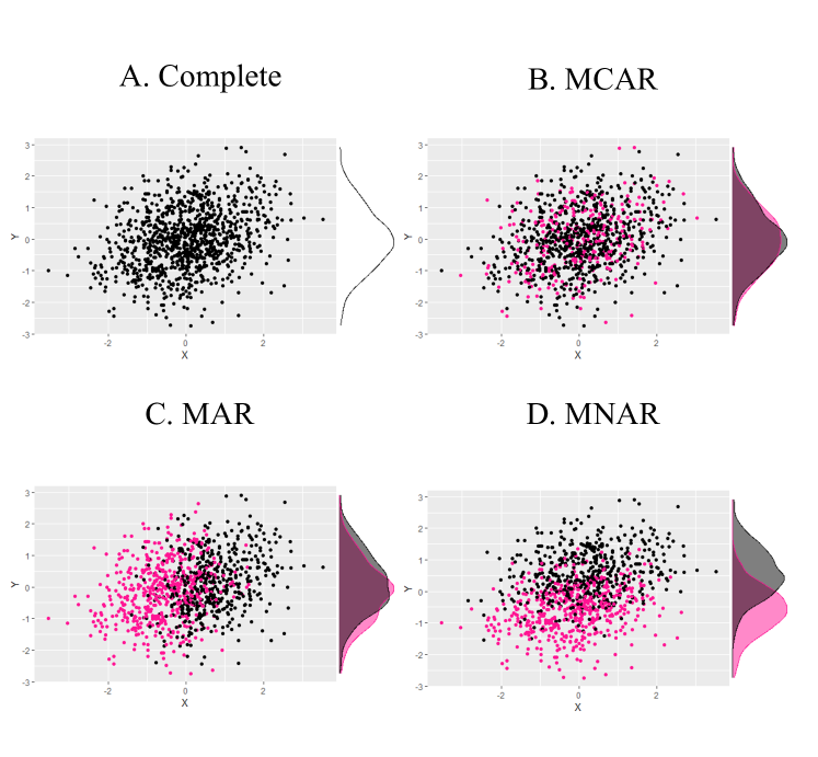
Figure 1: The above graphs show variables correlated at .3 with A. complete data, B. MCAR-deleted data, C. MAR-deleted data, and D. MNAR-deleted data. The black dots represent the data that is present in the sample and the pink dots represent data that is missing. Variable $Y$ is the variable with missing data (in B-D) and variable $X$ is a variable with complete data. Note that in Panel B, the marginal distributions of the MCAR missing data are the same as the marginal distributions of the non-missing data, while in Panel C and D, the marginal distributions of the non-missing data are considerably different from the original complete data marginal distribution.

This can be seen in Figure 1 where $Y$ is our variable with missingness, Panel A shows the complete data, and Panel B shows the MCAR data with the pink points as the missing data and the pink marginal distribution as the missing distribution (black is the observed data). First, notice that the missingness is equiprobable across the sample: there is no clustering dependent on $Y$ or $X$. In our example, this would mean our missingness is not related to SHAPS score, $Y$, or the additional predictor, $X$. Also notice how neatly the marginal density distributions of observed and missing data map onto each other. Recall, the distribution of the observed sample will be the same as the distribution of the missing sample, and we see that here. This plot demonstrates why MCAR missingness mechanisms are less problematic than the other missingness mechanisms, insofar as the marginal distribution of $Y$ does not change even in the face of missingness.

Take again the example of a study of anhedonia levels in a schizophrenia spectrum disorder sample. In this case, the study also collects a variable indicating whether the individuals have schizophrenia or schizoaffective-depressive subtype (characterized both by schizophrenic and depressive symptoms). The Beck Depression Inventory (BDI: Beck ., 1961) is also collected. On the day of data collection, most of the schizophrenia patients are in schizophrenia-specific therapy group and unavailable to participate. Depression is strongly correlated with anhedonia, (Martino ., 2018) so the missingness of the SHAPS score variable is related to the other variables, diagnosis and BDI, in that one would expect to see higher BDI scores in the schizoaffective sample than the schizophrenia sample. Hence, with the parts of the schizophrenia sample with low BDI scores missing SHAPS scores, we see MAR missingness. There is nuance here in that, although, the missingness mechanism is in line with the relationship among the variables, MAR is still possible when the prediction of missingness comes apart from predicting the value of the variable (though is still related to the missingness). Still, for the sake of this example, we consider the former case.

A MAR mechanism occurs when the missingness of a variable is related to the observed values of variables other than the outcome variable. MAR is similar to MCAR in that the missingness of a variable is not related to the value of the variable with missing data. As such, for MAR, although the missingness is systematic (Newman, 2014; Bhaskaran  Smeeth, 2014), the randomness of MAR arises in that once we condition on the other observed variables, the missingness is random.

Imagine in Figure 1.A and 1.C, Y is the SHAPS score and X is BDI score. Notice the clustering for the low levels of depression: the most missingness occurs in samples with low depression. Notice that here, unlike with an MCAR missingness mechanism, the distributions between observed and missing data begin to differ, and therefore the distribution of the observed data is not the same as the distribution of the complete data. This difference is the reason why MAR missing data leads to bias in modeling: The observed data is not representative of the actual population.

Returning to the above example, we again collect data on the SHAPS, but also age, sex, diagnosis, BDI, and time-in-hospital variables. Unfortunately, we miss the full SHAPS battery for some individuals. Upon reflection, we realize that people who are low on anhedonia are less likely to volunteer to fill out our measure because they are unlikely to seek help (and we are collecting in an in-patient unit). Thus, our missingness is directly related to the SHAPS itself, and our data is MNAR. Furthermore, for individuals in the observed sample and individuals in the missing data sample who share the same age, sex, diagnosis, and time-in-hospital, we see different distributions of SHAPS scores.

Now, imagine Y is SHAPS score and X is BDI for Figure 1.D. Unlike the previous example, we are hypothesizing that the missingness is related to the SHAPS score with those with low scores less likely to participate. We see this clustering in the graph in the negative values for the x-axis, showing that there is a pattern to the missingness. We see even greater differences in the marginal density distributions for observed and missing data. As with MAR, the differences in the marginal distributions of the observed data vs. complete data is showing that the observed data is not representative of the population when afflicted by MNAR missingness.

An important first step to handling missing data is to understand missing data mechanisms. Much missing data advice is aimed towards MCAR, MAR and cross-sectional data. In the next section, we will consider missing data in time series analysis, which includes novel missingness mechanisms in addition to the classical mechanisms of Rubin (1976), before continuing on to techniques that can be used to handle missing data in time series analysis.

1.2 MCAR, MAR, and MNAR for time series

The above mechanisms of missingness apply as well to time series data. Imagine you are interested about change in SHAPS scores over time. You visit the inpatient unit once a week to collect scores. Sometimes when you come, some patients are having recreation time. Thus, you have a time series of SHAPS scores with occasional missing points for each individual. This is a case of MCAR for time series: the missingness is not related to the score or other variables in the model.

Imagine the hospital has separate therapy groups for schizophrenia and schizoaffective-depressive subtype disorder, and they alternate meeting during your collection times. At some time points, you miss the schizophrenia sample and at others, you miss the schizoaffective-depressive subtype sample, resulting in missing observations across time. This is a case of MAR: the missingness is related to the variables without missingness, that is, diagnosis, but not the variable with missing, the SHAPS scores.

Unique to time series, time-dependent missing at random, TMAR, occurs when the missingness depends only on the time variable in the model. This differs from traditional MAR in that you see periodicity in missingness (e.g., missingness might increase during the evening) and, also, missingness on consecutive data points with TMAR missingness. This occurs commonly in EMA studies when data is collected on uneven schedules as the missingness may be dependent upon the the data collection schedule itself. For example, imagine we collect data throughout the day and include one late night time point. Patients who go to sleep early may be less likely to participate at this time point, and depending how close the preceding point is, we may see missingness in that point as well. Notice there will be periodicity in the missingness in that this particular point or points will be consistently missed (i.e., the early sleepers will consistently miss the late night time point resulting in a periodic pattern between days).

In addition, you collect SHAPS scores, age, sex, diagnosis, and time-in-hospital every week. You notice the hospital has an ”anhedonia support group” that meets sometimes when you collect. Thus, on those occasions, you miss collecting the data of those who attend this support group. You realize that this might be problematic for analysis because the missingness is related to the value of your SHAPS variable. This is a case of MNAR: the missingness of the missing variable, SHAPS scores, is related to the value of the missing variable.

A form of MNAR for time series, autoregressive TMAR or ATMAR, occurs when the missingness on a variable at time $t$ is dependent upon the previous values of the variable. It is similar to MNAR in that the variable with missingness is causing its own missingness, though it incorporates the autoregressive time-dependent relations of the variable over time. For example, consider collecting SHAPS scores at two time points. At the first time point, an individual has a high SHAPS score. At the second time point, the SHAPS score is missing. The researcher must answer the question: Is the high SHAPS score related to the later missing SHAPS score? If this answer is yes, then the missingness is ATMAR. If the answer is no, but the high SHAPS score is related to another variable in the model, including time, then the missingness would be MAR or TMAR. If the missingness is not related to any of the variables, which is typically unrealistic, the missingness would be MCAR.

In the context of EMA, these missing data mechanism occur with varying frequency. As with cross-sectional MCAR, time series MCAR is relatively rare as the criterion is difficult to meet. MAR and MNAR will occur in time series at the same frequencies as their cross-sectional counterparts, in both cases being relatively common. TMAR is the most commonly occurring missing data mechanism in EMA as it depends on the data collection schedule (and it is rare to have a perfect data collection schedule). Finally, ATMAR is common when there are time trends in EMA data.

While there are some commonalities between cross-sectional and time series missingness, time-dependent missingness is unique to time series analysis. Because of this, methods of missing data imputation differ between cross-sectional and time series data. This will be considered in the next section.

1.3 Missing data methods for time series

There are a number of methods proposed for handling missing data. The least sophisticated of these is known as listwise deletion, in which all variable values for a given participant at time $t$ are deleted if any one of those variables has missing data. Additionally, mean, mode, or median imputation is often used to replace the missing value with the relevant summary statistic. Generally, these methods are inappropriate for any form of missingness other than MCAR due to differences between the observed and complete distributions, but they are particularly unsuitable for time series data because they ignore the time-dependency of the data. Here,we will consider multiple imputation methods, which use information from the observed other variables in the model to inform the generation of the missing data imputation values, multiple imputation by chained equations (MICE: Ji ., 2018). We will also consider single imputation methods which take into account the temporal dependency in EMA data: the Kalman filter and a variety of methods using the Expectation Maximization algorithm (EM: Dempster ., 1977), chosen due to their citation popularity and the availability of $R$ packages.

1.4 MICE

MICE (Ji ., 2018) is a multiple imputation method in which missing data values are drawn through variable-by-variable iterations over conditional densities with Markov Chain Monte Carlo (MCMC) techniques. Mathematically, consider $\mathbf{Y}$, to be a matrix of dependent variables for all individuals and $\mathbf{X}$ to be a matrix of the covariates for all individuals. Then, $\mathbf{Y}_{o}$ and $\mathbf{X}_{o}$ are the observed variables and $\mathbf{Y}_{m}$ and $\mathbf{X}_{m}$ are the missing variables. With $\theta$ as the vector of unknown parameters, the $i$th iteration of the chained equation is a Gibbs sampler, a MCMC algorithm for sampling from a multivariate distribution, that iteratively draws from the distributions

$$\mathbf{\theta}_{i} \sim P(\mathbf{\theta}|\mathbf{Y}_{o},\mathbf{X}_{i-1})$$ (5)

$$\mathbf{Y}_{m(i)} \sim P(\mathbf{Y}|\mathbf{Y}_{o},\mathbf{X}_{i-1},\mathbf{\theta}_{i})$$ (6)

$$\mathbf{X}_{m(i)} \sim P(\mathbf{X}|\mathbf{X}_{o},\mathbf{Y}_{i},\mathbf{\theta}_{i})$$ (7)

Here, the draws for the missing variables, $Y_{m(i)}$ and $X_{m(i)}$ are conditional on the non-missing dependent and independent variables, respectively, and the complete imputed data from the independent and dependent variables, respectively, and the draws from the parameter distribution. It is assumed that the relations among the variables follow a general or generalized linear model, though there is flexibility depending on the distributional characteristics of the data. Another benefit of MICE is that, unlike many other imputation methods, it can handle a mix of variable types (e.g., continuous, ordinal, nominal, etc.).

The default imputation method in MICE for numerical variables is predictive mean matching (PMM: van Buuren  Groothuis-Oudshoorn, 2011; Rubin  Schenker, 1986; RJA. Little, 1988) . To summarize the relevant details of this approach, PMM begins by first fitting Bayesian regression models predicting the target variable $Y$ by the covariates $X$ (in this application, these are linear regression models) to obtain the posterior distributions of regression parameters. Then, for each given missing value of $Y$, $Y_{j}[mis]$, pairwise distances are calculated as $|X_{i}[obs]\hat{\beta}-X_{j}[mis]\dot{\beta}|$. From there, candidate observed values of $Y$ are selected from cases with the minimum calculated distance. The missing value $Y_{j}[mis]$ is then imputed by randomly sampling one of those observed values (with probability proportional to the distance metric). Note that this method imputes missing values with values drawn from observed data, rather than sampling from some theoretical distribution. In the context of the state-space models studied here, this implies that MICE, at least used in a typical manner, does not take into account any latent state information (which contrasts this approach with the Kalman filter described below). Also note that, by default, this approach does not account for temporal dependency when applied to timeseries data, as missing values are predicted by other variables at the same timepoint. However, by including lagged versions of variables as additional predictors, the PMM approach can include temporal information. We explore both the standard PMM and the use of lagged predictors in our simulation study.

Simulation studies on the procedure (Ji ., 2018) have shown recovery of point estimates with less bias than listwise deletion. MICE results in multiple imputed datasets, requiring the aggregation of results across datasets during analysis. It has also seen success with binary responses (Hardt ., 2013; Zaninotto  Sacker, 2017), in models with interactions (Zaninotto  Sacker, 2017), and when imputing missing scale items not the individual-level, but at the level of scale summaries (Plumpton ., 2016).

An alternative multiple imputation method not considered here is the the {Amelia} R package (Honaker ., 2011), which is able to fit polynomial trends to timeseries data. This would improve imputation in situations where there are clear polynomial trends, such as panel longitudinal studies, where the trajectory over time is often of greatest interest. However, Amelia II is limited to deterministic time trends, which are separate from the autoregressive effects of interest here. Hence, we do not consider Amelia here.

As MICE is a multiple imputation method, a method that imputes $i$ many datasets, it requires some way of compiling and comparing the multiple imputed data sets. The standard way appears in Rubin (1996) and is summarized here (see Supplemental Material for details). The actual posterior distribution defined by $\theta$ is the average of the posterior predictive distributions of the missing data, given by the observed data. It follows that the posterior mean of the distribution defined by $\theta$ is the average of the posterior means of the multiply imputed data sets and the variance of the posterior distribution defined by $\theta$ is the average of the variances of the multiply imputed data sets plus the variance of the multiply imputed data sets. In this way, $i$ many data sets which have been multiply imputed can be analyzed as one data set.

1.5 Expectation Maximization

The EM algorithm is a general purpose estimating technique that was originally developed in the context of estimating missing data (Dempster ., 1977). The EM algorithm can be used in tandem with single or multiple imputation. Instead of directly estimating the values of the missing data elements, the approach of Junger  Ponce de Leon (2015) uses the EM algorithm to estimate the distributional characteristics of the missing data, and then to sample from that distribution.

The approach of Junger  Ponce de Leon (2015) can be summarized as follows: Define a vector of all the variables at time t, $x_{t}$, and split it so that the first $n$ variables are the ones with missing values and the remaining, up to $d$, are the observed values, $\mathbf{x_{t}}=(x_{t1},x_{t2},\dots,x_{tn},x_{tn+1},\dots,x_{td})$. As such, there are two mean parameters, one for the missing values at time $t$ and the other for the observed values, $\begin{pmatrix}\mu_{tm}\\ \mu_{to}\end{pmatrix}$ (where $\mu_{tm}$ is the mean for the missing values and $\mu_{to}$ is the mean for the observed values) and a $2\times 2$ covariance matrix defined over some set of time windows to allow for non-stationarity in the time series. For simplicity’s sake, we suppress the window notation, and denote the covariance matrix as $\sigma^{2}$.

At each expectation step of the EM algorithm, missing values ($x_{t1}$) are imputed with the following expected value:

$$x_{t1}=E[X_{t}1|x_{t2},\mu_{t},\Sigma]=\mu_{tm}+\Sigma_{12}\sigma_{22}^{-1}(x_{t2}-\mu_{to})$$ (8)

Following the imputation of the missing values during each expectation step, maximum likelihood estimates of $\mu_{t}m,\mu_{t}o$ and $\sigma^{2}$ are computed, with $\mu_{t}m$ and $\mu_{t}o$ being computed using a specific level estimation model.

There are a number of ways of estimating $\mu_{t}m$ and $\mu_{t}o$. Indeed, Junger  Ponce de Leon (2015) note that any time series filtering method can be used. They provide three different estimation models that are tested here. First, an autoregressive integrated moving average (ARIMA) model can be used by finding the d-th order difference and using the mean estimate of the one-step ahead prediction. Second, a natural cubic spline with curve, $g$, can find an initial mean as $g(x_{t})$ gives an estimate. Finally, Junger  Ponce de Leon (2015) propose the use of a generalized additive model (GAM: Trevor Hastie  Robert Tibshirani, 1986), which are flexible regression type models that allow for non-linear relations to be automatically fit.

1.6 Kalman Filtering

Kalman filtering is a baseline method for handling multivariate missing time series data modeled as a state-space model. While it is not a missing data imputation method in the traditional sense in that it does not impute values for the observed variables, it is used as a solution to issues arising from missing data. It is a natural part of estimating state-space models, as state-space models require estimates of the latent states (which is provided by filtering). However, Kalman filtering also provides a missing data imputation method at the level of states as it allows for the prediction of states from previous values. This method, at time $t$, recursively estimates latent states, $x_{t}$, and a covariance matrix of states, $P_{t}$. For the time update $x_{t}$ and $P_{t}$ are updated as follows:

$$\bar{\mathbf{P}}_{t+1}=\mathbf{A}\mathbf{P}_{t}\mathbf{A}^{\prime}+\mathbf{Q}$$ (9)

$$\bar{\mathbf{x}}_{t+1}=\mathbf{A}\mathbf{x}_{t}$$ (10)

and for the measurement update, they are updated as follows:

$$\mathbf{P}_{t+1}=[(\bar{\mathbf{P}}_{t+1})^{-1}+\mathbf{H}^{\prime}\mathbf{R}^{-1}_{t+1}\mathbf{H}]^{-1}$$ (11)

$$\bar{\mathbf{x}}_{t+1}=\bar{\mathbf{x}}_{t+1}+\mathbf{P}_{t+1}\mathbf{H}^{\prime}\mathbf{R}^{-1}(\mathbf{z}_{t+1}-\mathbf{H}_{t+1}\bar{\mathbf{x}}_{t+1}$$ (12)

We may be concerned about the measurement update due to its reliance on $z_{t+1}$, which may be missing given our current set-up. However, notice that the time update does not depend on the observed variables. Thus, $X_{t}$ and $P_{t}$ can be updated even in the presence of missing data if we forgo the measurement update and rely, merely, on the time update. Hence, we can still use the Kalman filter on missing data with our updates occurring at the time level. Note that Kalman filtering is a single pass imputation method that is purely based on the estimated state dynamics, rather than any information being used from other variables in the system. For the Kalman filter, the standard errors are not adjusted as the state values are being estimated, not the parameter values. Thus, the standard errors will be larger than with complete data, simply because there is less data to inform them. In this simulation, this will be used as our baseline method.

The preceding missing data imputation methods provide both single and multiple imputation approaches to time series data, taking into account the time dependencies characteristic of such data. In the context of cross-sectional data, multiple imputation tends to be recommended over single imputation (Sinharay ., 2001). In the case of single imputation, point estimates cannot take into account the uncertainty of the missing data values, resulting in standard errors that are too small, while, for multiple imputation, as $i$ many data sets are estimated, such uncertainty can be accounted for (Donders ., 2006). In the proceeding section, we propose a simulation to examine if this recommendation holds for multivariate time series data.

2 Methods

We examined how missing data mechanisms impact the recovery of parameter estimates, by performing a Monte-Carlo simulation. In this simulation, data was generated and a portion of the data was deleted to create MCAR, MAR, TMAR, ATMAR, and MNAR samples with $\beta$ coefficients from the corresponding logistic regressions found via grid search. The resulting data sets were analyzed in a discrete time continuous measure state-space model with Kalman filtering as a baseline method and compared with multivariate time series data imputation methods

2.1 Data Generating Model

The data generating model for this simulation is the discrete time state-space model with linearly related normally distributed states and normally distributed observations. This model can be viewed as a dynamic factor model. To keep the simulation simple, we simulated a 2 state, 3 indicators per state model of the following form:

$$\mathbf{x}_{t+1}=\mathbf{A}\mathbf{x}_{t}+\mathbf{v}_{t}$$ (13)

$$\mathbf{v}_{t}\sim N_{p}(\mathbf{0}_{p},\mathbf{Q})$$ (14)

$$\mathbf{z}_{t}=\mathbf{H}\mathbf{x}_{t}+\mathbf{w}_{t}$$ (15)

$$\mathbf{w}_{t}\sim N_{p}(\mathbf{0}_{p},\mathbf{R})$$ (16)

where $x_{t}$ is the $2\times T$ matrix of states $A$ is the $2\times 2$ matrix of transition coefficients, $0_{p}$ is the 2x1 mean zero vector, $Q$ is the $p\times p$ covariance matrix for the state error, $z$ is the measurement at time t, $H$ is the $6\times 2$ matrix that maps states to measurements, and $R_{t}$ is the $6\times 6$ covariance matrix for measurement error.

2.2 Conditions

There were be 2 states with 3 items per state. The state error covariance $Q$ is set to identity for all conditions. Measurement error is operationalized by choosing values in the error covariance matrix $\mathbf{R}=\begin{pmatrix}\sigma^{2}&0\\ 0&\sigma^{2}\end{pmatrix}$ and the loading matrix $\mathbf{H}$ matrix is of the form $\begin{pmatrix}\lambda&\lambda&\lambda&0&0&0\\ 0&0&0&\lambda&\lambda&\lambda\end{pmatrix}$ such that the following equality holds: $\sigma^{2}+\lambda^{2}=1$. We varied the measurement error in 2 conditions: low ($\sigma^{2}=.25,\lambda^{2}=.75$) and high measurement error ($\sigma^{2}=.75,\lambda^{2}=.25$)

The A matrix (containing autoregressive and crosslagged effects) takes the form $\begin{pmatrix}\alpha&\gamma\\ 0&\alpha\end{pmatrix}$, where $\alpha$ $\in$ $\{$.2,.7$\}$ to examine differing strengths of autoregressive relations and $\gamma$ $\in$ $\{$0, .15, .3$\}$ (fully crossed) to examine how missingness mechanisms interact with cross-lagged relations (no relation between states, moderate relation between states, and strong relationship between states). The above values were chosen to avoid having extreme values (i.e., the values are neither too small nor too large).

2.2.1 MCAR

For the MCAR mechanism, we simulated 2 levels of missingness: $15\%$ and $30\%$. All indicators for the state $x_{1}$ with the targeted indices were set to NA, corresponding with all direct information about state $x_{1}$ being missing.

2.2.2 MAR, TMAR, and ATMAR

For the MAR data, a logistic regression was run with the two states as predictors with positive coefficients, then the probability of missingness was set to

$$p(y_{1t},y_{2t},y_{3t}=NA)=\frac{1}{1+\exp(\beta_{0}+\beta_{MAR}x_{2t})}$$

Indices of missingness were chosen based on the probabilities of missingness, $\beta_{0}\in\{4,1.5\}$ and $\beta_{MAR}\in\{-3.5,-3\}$ for 15% 30% missingness at +1$\sigma^{2}$ above the mean of $x_{2}$, respectively.

For TMAR data, we assumed there are 50 days with 10 time points per day, and an auxiliary variable $D\in\{1:10\}$ was calculated. A logistic regression for the probability of state $x_{1}$ indicators ($y_{1t},y_{2t},y_{3t}$) being missing as a function of $D$ is

$$p(y_{1t},y_{2t},y_{3t}=NA)=\frac{1}{1+\exp{\beta_{0}+\beta_{TMAR}D_{t}}}$$

with $\beta_{0}\in\{3,2\}$ and $\beta_{TMAR}\in\{-.2,-.2\}$ for 15% 30% missingness for $D=1$, respectively.

For an ATMAR condition, we used a logistic function with the the probability of missingness set to

$$p(y_{1t},y_{2t},y_{3t}=NA)=\frac{1}{1+\exp{\beta_{0}+\beta_{ATMAR}x_{1(t-1)}}}$$

with $\beta_{0}\in\{4,1,5\}$ and $\beta_{ATMAR}\in\{-3.5,-3\}$ for 15% 30% missingness at $x_{1}=1$, respectively. Note, this condition, while labeled as MAR, mixes MAR and MNAR mechanisms, as the values for $y_{1[t-1]},y_{2[t-1]},y_{3[t-1]}$ can be observed or missing.

2.2.3 MNAR

Recall that the difference between MAR and MNAR is that in MAR the missingness is dependent on other variables and, in MNAR, the missingness is dependent on the variable from which the data is missing. Thus, we used a similiar model of generating missing data for MAR and MNAR. We set up an logistic regression with our variable of interest as our dependent variable and our variable of interest as our predictor, then, the probability of missingness was set to

$$p(y_{1t},y_{2t},y_{3t}=NA)=\frac{1}{1+\exp{\beta_{0}+\beta_{MNAR}X_{1}t}}$$

with $\beta_{0}\in\{4,1.5\}$ and $\beta_{MNAR}\in\{-3.5,-3\}$ 15% and 30% missingness at $X_{1}=1$, respectively.

2.3 Missing data imputation

The missing data imputation methods that were used were the Kalman filter ({dlm} R package: Petris, 2010), MICE-def and MICE-t ({mice} R package: van Buuren  Groothuis-Oudshoorn, 2011), and the EM algorithm with initializations of ARIMA, regression, and natural cubic spline ({mtsdi} R package: Junger  Ponce de Leon, 2015)). Default settings were used in all cases except MICE-t, which uses a lagged matrix to predict the values of $z$ at time $t$ from the values of $z$ at time $t-1$ (as opposed to the Kalman filter which predicts time $t$ states from time $t-1$ states). For MICE-def, the imputation models for $z_{1},z_{2}$ and $z_{3}$ were calculated using only $z_{4},z_{5}$ and $z_{6}$ (as each of $z_{1},z_{2},z_{3}$ are set as missing simultaneously) at the same time point, and for MICE-t, this pattern of prediction is used from the previous time point (i.e $\mathbf{z}_{[1-3]t}$ as a function of $\mathbf{z}_{[1-6]t-1}$). With MICE-def, in order for $z_{4}$-$z_{6}$ to have use in imputation, they need to have to have cross-sectional predictive ability on $z_{1}$-$z_{3}$. This only occurs when $\gamma$ is non-zero, and, even then, the dependence would be weak.

2.4 Simulation overview

A $2(\text{measurement error conditions})\times 2(\alpha\text{ conditions})\times 3(\gamma\text{ conditions})$ cell design was run for 100 replications for each cell to produce the raw timeseries (before missingness), with 500 timepoints per replication. The $10$ conditions of missingness mechanisms were then applied to the previously simulated raw data. For each of the 10 datasets with missing data per replication, the 7 missing data imputation methods were applied. For missing data imputation methods that generated multiple imputed datasets (i.e., MICE), 10 imputed datasets were generated, and parameter estimates/standard errors will be combined according to the standard practice of Rubin (1996).

2.5 Simulation Models and Outcomes

Using the {dlm} R package (Petris, 2010), discrete time normally distributed state/measurement state-space models described in Equations 12-15 were fit, with the following free and fixed parameters: $\hat{\mathbf{A}}=\begin{pmatrix}\hat{\alpha}&\hat{\gamma}\\ 0&\hat{\alpha}\end{pmatrix}$, $\hat{\mathbf{H}}=\begin{pmatrix}\hat{\lambda}_{1}&\hat{\lambda}_{2}&\hat{\lambda}_{3}&0&0&0\\ 0&0&0&\hat{\lambda}_{4}&\hat{\lambda}_{5}&\hat{\lambda}_{6}\end{pmatrix}$, $\hat{\mathbf{R}}=\begin{pmatrix}\hat{\sigma^{2}}&0\\ 0&\hat{\sigma^{2}}\end{pmatrix}$ and for identification purposes, the state error covariance matrix is fixed at $\mathbf{I}_{2}$. Parameter values were chosen based on the principle that they are not extreme values (i.e., they are neither too weak or too strong).

The following were computed for each cell for $\alpha$, $\gamma$, $\sigma^{2}$ and $\lambda^{2}$.

2.5.1 Median bias

$$\Delta\theta=\text{Median}(\theta-\hat{\theta})$$

where the $\theta$ are the true values of the parameter that are the assumed matrices and $\hat{\theta}$ are the estimated parameters. Bias is found, then the median of each condition is found.

2.5.2 Median absolute relative bias

$$\Delta\theta_{Rel}=\frac{|\theta-\hat{\theta}|}{\theta}$$

where the $\theta$ and $\hat{\theta}$ values are as above. Relative bias is found, then the median of each condition is found.

2.5.3 Standard error and coverage

The bias in standard error, $SE$, of estimates is contained in the Supplementary Materials.

Confidence intervals will be calculated as follows:

$$[\hat{\theta}-1.96SE,\hat{\theta}+1.96SE]$$

where $\overline{x}$ is the mean of a condition and $SE$ is defined as above. The coverage for a given parameter $\theta$ is the number of replications where the above confidence interval contains the true parameter $\theta$.

3 Results

Table 1: Median bias for each condition (i.e., ”Variable”) across all other conditions for each parameter.

Variable	$\alpha$	$\gamma$	$\lambda^{2}$	$\sigma^{2}$
$\alpha$ = .2	0.001	0.029	0.011	0.036
$\alpha$ = .7	0.036	0.022	0.008	0.028
$\gamma$ = 0	0.019	-0.001	0.008	0.032
$\gamma$ = .15	0.02	0.029	0.01	0.032
$\gamma$ = .3	0.014	0.062	0.01	0.031
Complete	0.003	-0.001	0.002	0.003
MCAR	0.051	0.014	0.009	0.037
TMAR	0.049	0.016	0.01	0.036
MAR	0.047	0.016	0.007	0.026
MNAR	-0.042	0.052	0.012	0.037
ATMAR	-0.037	0.054	0.012	0.038
None	0.004	0.001	0.002	0.003
K	-0.01	0.009	0.004	0.002
MICE-def	0.105	0.041	0.008	-0.001
MICE-t	0.079	0.031	0.006	0
EM-ARIMA	-0.015	0.032	0.017	0.087
EM-Spline	-0.05	0.031	0.014	0.076
EM-Regression	0.063	0.01	0.012	0.073
Missingness = .15	0.026	0.02	0.01	0.028
Missingness = .3	0.002	0.031	0.009	0.039
$\sigma^{2}$ = .25	0.021	0.025	0.008	0.02
$\sigma^{2}$ = .75	0.012	0.024	0.012	0.066
$\lambda^{2}$ = .25	0.012	0.024	0.012	0.066
$\lambda^{2}$ = .75	0.021	0.025	0.008	0.02

Table 2: Median bias for $\alpha_{11}$, $\sigma^{2}_{1}$, $\sigma^{2}_{2}$, $\sigma^{2}_{3}$, $\lambda_{11}^{2}$, $\lambda_{12}^{2}$, and $\lambda_{13}^{2}$ for the $\gamma$ = 0 and 30% missingness condition. MCAR, ATMAR, and MAR were excluded as TMAR behave similarly to MCAR and MAR and ATMAR performs similarly to MNAR. Outliers, defined as the absolute value of the bias being greater than 1, were excluded (6 points)

Missingness	Imputation	True $\alpha$	True $\lambda^{2}$	$\alpha_{11}$	$\sigma^{2}_{1}$	$\sigma^{2}_{2}$	$\sigma^{2}_{3}$	$\lambda_{11}^{2}$	$\lambda_{12}^{2}$	$\lambda_{13}^{2}$
MNAR	MICE-t	0.2	0.75	-0.135	-0.004	-0.002	-0.003	0.207	0.183	0.194
TMAR	MICE-t	0.2	0.75	0.095	-0.001	-0.001	0.002	0.016	-0.002	0.002
MNAR	MICE-t	0.7	0.75	0.129	0.004	-0.008	0	-0.046	-0.036	-0.044
TMAR	MICE-t	0.7	0.75	0.337	0.005	0.006	-0.001	-0.454	-0.461	-0.461
MNAR	MICE-t	0.2	0.25	-0.264	-0.031	-0.019	-0.023	0.126	0.141	0.13
TMAR	MICE-t	0.2	0.25	0.093	0.024	0.009	-0.002	0.006	-0.009	0.005
MNAR	MICE-t	0.7	0.25	-0.049	-0.037	-0.038	-0.058	0.111	0.112	0.114
TMAR	MICE-t	0.7	0.25	0.33	-0.01	0.007	0.003	-0.148	-0.152	-0.166
MNAR	MICE-def	0.2	0.75	-0.144	0.005	0.004	0.003	0.192	0.187	0.194
TMAR	MICE-def	0.2	0.75	0.092	0.008	0.005	-0.005	0.005	0.012	0.01
MNAR	MICE-def	0.7	0.75	0.153	-0.007	0	0.011	-0.056	-0.059	-0.071
TMAR	MICE-def	0.7	0.75	0.333	0.004	0	0.009	-0.433	-0.452	-0.454
MNAR	MICE-def	0.2	0.25	-0.311	-0.041	-0.025	-0.016	0.144	0.144	0.129
TMAR	MICE-def	0.2	0.25	0.099	0.004	0.017	0.001	-0.015	-0.011	-0.001
MNAR	MICE-def	0.7	0.25	-0.035	-0.045	-0.035	-0.034	0.083	0.099	0.099
TMAR	MICE-def	0.7	0.25	0.306	0.017	-0.004	0.015	-0.159	-0.147	-0.159
MNAR	K	0.2	0.75	-0.197	-0.006	-0.004	0.005	0.216	0.221	0.21
TMAR	K	0.2	0.75	-0.008	0.002	0.001	-0.002	0.016	0.015	0.005
MNAR	K	0.7	0.75	-0.005	0.011	0.006	-0.008	0.221	0.213	0.227
TMAR	K	0.7	0.75	0.007	0.004	0.007	0.005	0.001	0.002	0.013
MNAR	K	0.2	0.25	-0.355	-0.022	-0.018	-0.017	0.134	0.128	0.124
TMAR	K	0.2	0.25	-0.011	0.016	0.014	0.014	-0.001	0.012	0.019
MNAR	K	0.7	0.25	-0.093	-0.015	-0.024	-0.006	0.127	0.129	0.127
TMAR	K	0.7	0.25	0.001	-0.002	0.007	0.017	0.011	0.006	0.007
MNAR	EM-Spline	0.2	0.75	-0.262	0.078	0.08	0.08	0.368	0.374	0.373
TMAR	EM-Spline	0.2	0.75	0.035	0.066	0.069	0.076	0.229	0.229	0.224
MNAR	EM-Spline	0.7	0.75	-0.092	0.04	0.05	0.056	0.424	0.419	0.42
TMAR	EM-Spline	0.7	0.75	-0.067	0.05	0.042	0.046	0.204	0.194	0.199
MNAR	EM-Spline	0.2	0.25	-0.699	0.203	0.204	0.198	0.233	0.232	0.231
TMAR	EM-Spline	0.2	0.25	0.053	0.228	0.23	0.236	0.076	0.074	0.072
MNAR	EM-Spline	0.7	0.25	-0.201	0.233	0.225	0.224	0.202	0.206	0.202
TMAR	EM-Spline	0.7	0.25	-0.098	0.183	0.185	0.179	0.091	0.094	0.101
MNAR	EM-Regression	0.2	0.75	-0.231	0.071	0.066	0.069	0.338	0.34	0.34
TMAR	EM-Regression	0.2	0.75	0.063	0.067	0.074	0.069	0.194	0.185	0.197
MNAR	EM-Regression	0.7	0.75	0.042	0.071	0.065	0.073	0.188	0.194	0.192
TMAR	EM-Regression	0.7	0.75	0.231	0.072	0.074	0.063	-0.081	-0.084	-0.072
MNAR	EM-Regression	0.2	0.25	-0.583	0.158	0.162	0.168	0.214	0.22	0.209
TMAR	EM-Regression	0.2	0.25	0.071	0.206	0.196	0.199	0.067	0.069	0.075
MNAR	EM-Regression	0.7	0.25	-0.119	0.197	0.171	0.172	0.157	0.166	0.155
TMAR	EM-Regression	0.7	0.25	0.186	0.195	0.203	0.198	-0.004	-0.005	-0.01
MNAR	EM-ARIMA	0.2	0.75	-0.25	0.081	0.08	0.084	0.368	0.36	0.362
TMAR	EM-ARIMA	0.2	0.75	-0.008	0.077	0.074	0.076	0.219	0.218	0.226
MNAR	EM-ARIMA	0.7	0.75	-0.051	0.083	0.084	0.081	0.36	0.37	0.367
TMAR	EM-ARIMA	0.7	0.75	0.012	0.054	0.051	0.059	0.141	0.149	0.139
MNAR	EM-ARIMA	0.2	0.25	-0.629	0.188	0.206	0.207	0.231	0.22	0.215
TMAR	EM-ARIMA	0.2	0.25	0.014	0.222	0.24	0.214	0.074	0.07	0.087
MNAR	EM-ARIMA	0.7	0.25	-0.159	0.241	0.247	0.244	0.174	0.178	0.175
TMAR	EM-ARIMA	0.7	0.25	0.044	0.216	0.213	0.202	0.055	0.055	0.058

Table 3: Median bias for $\alpha_{11}$, $\sigma^{2}_{1}$, $\sigma^{2}_{2}$, $\sigma^{2}_{3}$, $\lambda_{11}^{2}$, $\lambda_{12}^{2}$, and $\lambda_{13}^{2}$ for the $\gamma$ = 0.3 and 30% missingness condition. MAR, ATMAR, and MCAR were excluded as TMAR behaves similarly to MCAR and MAR and ATMAR performs similarly to MNAR. Outliers, defined as the absolute value of the bias being greater than 1, were excluded (6 points)

Missingness	Imputation	True $\alpha$	True $\lambda^{2}$	$\alpha_{11}$	$\sigma^{2}_{1}$	$\sigma^{2}_{2}$	$\sigma^{2}_{3}$	$\lambda_{11}^{2}$	$\lambda_{12}^{2}$	$\lambda_{13}^{2}$
MNAR	MICE-t	0.2	0.75	-0.156	0.006	-0.004	-0.001	0.164	0.166	0.151
TMAR	MICE-t	0.2	0.75	0.096	0	0.003	0.004	-0.031	-0.049	-0.03
MNAR	MICE-t	0.7	0.75	0.09	-0.002	0	0.003	-0.229	-0.209	-0.236
TMAR	MICE-t	0.7	0.75	0.331	-0.001	-0.004	0.002	-0.759	-0.739	-0.771
MNAR	MICE-t	0.2	0.25	-0.308	-0.034	-0.033	-0.033	0.129	0.132	0.133
TMAR	MICE-t	0.2	0.25	0.107	0.021	0.022	0.02	-0.006	-0.003	-0.024
MNAR	MICE-t	0.7	0.25	-0.02	-0.032	-0.042	-0.033	0.004	0.017	0.015
TMAR	MICE-t	0.7	0.25	0.337	0.018	-0.024	-0.002	-0.257	-0.233	-0.244
MNAR	MICE-def	0.2	0.75	-0.144	0.003	0.005	0	0.165	0.161	0.164
TMAR	MICE-def	0.2	0.75	0.102	0.001	0.003	-0.001	-0.03	-0.028	-0.043
MNAR	MICE-def	0.7	0.75	0.094	-0.004	0.004	0	-0.199	-0.216	-0.233
TMAR	MICE-def	0.7	0.75	0.336	0.003	0.01	0.001	-0.717	-0.724	-0.734
MNAR	MICE-def	0.2	0.25	-0.313	-0.044	-0.04	-0.026	0.131	0.136	0.135
TMAR	MICE-def	0.2	0.25	0.099	-0.001	0.001	0.006	-0.007	-0.015	-0.005
MNAR	MICE-def	0.7	0.25	-0.057	-0.039	-0.062	-0.037	0.024	0.035	0.025
TMAR	MICE-def	0.7	0.25	0.325	0.003	-0.009	0.016	-0.252	-0.233	-0.246
MNAR	K	0.2	0.75	-0.197	0.004	-0.002	0.003	0.211	0.207	0.206
TMAR	K	0.2	0.75	0	-0.002	-0.011	0.005	0.007	0.021	0.011
MNAR	K	0.7	0.75	-0.005	0.003	0	-0.001	0.167	0.173	0.176
TMAR	K	0.7	0.75	0.009	0.001	-0.004	0.004	0.012	-0.005	0
MNAR	K	0.2	0.25	-0.292	0.008	-0.01	-0.007	0.098	0.105	0.095
TMAR	K	0.2	0.25	0.008	0.013	0.009	0.016	0.005	0.002	-0.001
MNAR	K	0.7	0.25	-0.054	0.001	-0.004	0.009	0.084	0.078	0.087
TMAR	K	0.7	0.25	-0.007	0	0.017	0.003	0.003	0.001	0
MNAR	EM-Spline	0.2	0.75	-0.279	0.081	0.078	0.081	0.356	0.343	0.346
TMAR	EM-Spline	0.2	0.75	0.013	0.065	0.068	0.069	0.211	0.207	0.207
MNAR	EM-Spline	0.7	0.75	-0.103	0.029	0.03	0.035	0.366	0.365	0.363
TMAR	EM-Spline	0.7	0.75	-0.051	0.047	0.042	0.045	0.093	0.095	0.088
MNAR	EM-Spline	0.2	0.25	-0.767	0.205	0.189	0.2	0.243	0.242	0.242
TMAR	EM-Spline	0.2	0.25	0.014	0.238	0.212	0.216	0.058	0.069	0.074
MNAR	EM-Spline	0.7	0.25	-0.198	0.207	0.217	0.215	0.187	0.183	0.185
TMAR	EM-Spline	0.7	0.25	-0.058	0.159	0.158	0.182	0.072	0.068	0.065
MNAR	EM-Regression	0.2	0.75	-0.227	0.065	0.071	0.07	0.308	0.303	0.314
TMAR	EM-Regression	0.2	0.75	0.063	0.065	0.073	0.066	0.167	0.157	0.164
MNAR	EM-Regression	0.7	0.75	0.249	0.051	0.061	0.071	-0.771	-0.86	-0.81
TMAR	EM-Regression	0.7	0.75	0.329	0.075	0.062	0.069	-0.751	-0.759	-0.75
MNAR	EM-Regression	0.2	0.25	-0.448	0.187	0.164	0.167	0.172	0.177	0.171
TMAR	EM-Regression	0.2	0.25	0.098	0.198	0.21	0.22	0.062	0.06	0.058
MNAR	EM-Regression	0.7	0.25	0.461	0.21	0.173	0.169	-0.133	-0.238	-0.183
TMAR	EM-Regression	0.7	0.25	0.339	0.211	0.19	0.202	-0.159	-0.151	-0.156
MNAR	EM-ARIMA	0.2	0.75	-0.273	0.086	0.086	0.082	0.345	0.353	0.364
TMAR	EM-ARIMA	0.2	0.75	-0.001	0.071	0.075	0.075	0.205	0.208	0.206
MNAR	EM-ARIMA	0.7	0.75	-0.08	0.079	0.078	0.086	0.305	0.306	0.308
TMAR	EM-ARIMA	0.7	0.75	-0.006	0.045	0.038	0.047	0.088	0.085	0.083
MNAR	EM-ARIMA	0.2	0.25	-0.523	0.206	0.205	0.209	0.193	0.194	0.187
TMAR	EM-ARIMA	0.2	0.25	-0.011	0.226	0.218	0.222	0.072	0.083	0.076
MNAR	EM-ARIMA	0.7	0.25	-0.158	0.24	0.258	0.26	0.15	0.153	0.149
TMAR	EM-ARIMA	0.7	0.25	0.003	0.199	0.182	0.19	0.037	0.044	0.05

Table 4: Coverage, or percentage of the true parameters which fall within the confidence interval, for $\alpha$, $\gamma$, and $\lambda^{2}$ for the $\gamma$ = 0 and 30% missingness condition. MCAR and MAR were excluded as it behaves similarly to TMAR, and ATMAR was excluded as they behave similarly to MNAR.

Missingness	Imputation	True $\alpha$	True $\lambda^{2}$	$\alpha$	$\gamma$	$\lambda^{2}$
TMAR	K	0.2	0.75	96	94	48.667
TMAR	K	0.2	0.25	88	96	46
TMAR	K	0.7	0.75	91	96	48
TMAR	K	0.7	0.25	94	96	34
TMAR	MICE-def	0.2	0.75	77	99	56.667
TMAR	MICE-def	0.2	0.25	93	97	45.333
TMAR	MICE-def	0.7	0.75	0	93	33.333
TMAR	MICE-def	0.7	0.25	2	94	33.333
TMAR	MICE-t	0.2	0.75	73	96	54.667
TMAR	MICE-t	0.2	0.25	98	99	46.333
TMAR	MICE-t	0.7	0.75	0	98	33.333
TMAR	MICE-t	0.7	0.25	1	94	33.333
TMAR	EM-ARIMA	0.2	0.75	83	96	84.667
TMAR	EM-ARIMA	0.2	0.25	84.848	98.99	49.832
TMAR	EM-ARIMA	0.7	0.75	88.889	98.99	82.828
TMAR	EM-ARIMA	0.7	0.25	82	94	34.333
TMAR	EM-Spline	0.2	0.75	81	97	80.333
TMAR	EM-Spline	0.2	0.25	91	98	48.667
TMAR	EM-Spline	0.7	0.75	43	98	88
TMAR	EM-Spline	0.7	0.25	32	90	38.333
TMAR	EM-Regression	0.2	0.75	71	95	86.333
TMAR	EM-Regression	0.2	0.25	84	94	49.667
TMAR	EM-Regression	0.7	0.75	0	80	37.333
TMAR	EM-Regression	0.7	0.25	20	81	33.667
MNAR	K	0.2	0.75	15	91	88.667
MNAR	K	0.2	0.25	33	96	58
MNAR	K	0.7	0.75	90	95	84
MNAR	K	0.7	0.25	60	98	71
MNAR	MICE-def	0.2	0.75	28	97	96
MNAR	MICE-def	0.2	0.25	84	100	80.667
MNAR	MICE-def	0.7	0.75	13	97	49.333
MNAR	MICE-def	0.7	0.25	80	97	72.667
MNAR	MICE-t	0.2	0.75	37	99	94
MNAR	MICE-t	0.2	0.25	74.49	100	78.571
MNAR	MICE-t	0.7	0.75	15	98	51.333
MNAR	MICE-t	0.7	0.25	85	100	77.667
MNAR	EM-ARIMA	0.2	0.75	1	99	6.667
MNAR	EM-ARIMA	0.2	0.25	15	99	42
MNAR	EM-ARIMA	0.7	0.75	66.667	95.96	3.704
MNAR	EM-ARIMA	0.7	0.25	22	99	70.667
MNAR	EM-Spline	0.2	0.75	1	96	4
MNAR	EM-Spline	0.2	0.25	13	99	40
MNAR	EM-Spline	0.7	0.75	23	94	0.667
MNAR	EM-Spline	0.7	0.25	5	100	69.333
MNAR	EM-Regression	0.2	0.75	10	98	15.667
MNAR	EM-Regression	0.2	0.25	22.222	94.949	33.67
MNAR	EM-Regression	0.7	0.75	62	87	51
MNAR	EM-Regression	0.7	0.25	29.167	88.298	62.937

Table 5: Coverage, or percentage of the true parameters which fall within the confidence interval, for $\alpha$, $\gamma$, and $\lambda^{2}$ for the $\gamma$ = 0.3 and 30% missingness condition. MCAR and MAR were excluded as they behave similarly to TMAR, and ATMAR was excluded as it behaves similarly to MNAR.

Missingness	Imputation	True $\alpha$	True $\lambda^{2}$	$\alpha$	$\gamma$	$\lambda^{2}$
TMAR	K	0.2	0.75	96	97	51.333
TMAR	K	0.2	0.25	91	93	40.333
TMAR	K	0.7	0.75	97	98	44
TMAR	K	0.7	0.25	94	95	33.667
TMAR	MICE-def	0.2	0.75	61	72	43.667
TMAR	MICE-def	0.2	0.25	93	89	38.333
TMAR	MICE-def	0.7	0.75	0	65	33.333
TMAR	MICE-def	0.7	0.25	0	90	33.333
TMAR	MICE-t	0.2	0.75	74	70	45
TMAR	MICE-t	0.2	0.25	90	96	38.333
TMAR	MICE-t	0.7	0.75	0	59	33.333
TMAR	MICE-t	0.7	0.25	0	81	33.333
TMAR	EM-ARIMA	0.2	0.75	81	83	89.667
TMAR	EM-ARIMA	0.2	0.25	85.859	91.919	46.801
TMAR	EM-ARIMA	0.7	0.75	88.889	55.556	64.983
TMAR	EM-ARIMA	0.7	0.25	76	89	33.333
TMAR	EM-Spline	0.2	0.75	72	69	85.333
TMAR	EM-Spline	0.2	0.25	93	92	43.333
TMAR	EM-Spline	0.7	0.75	57	57	66
TMAR	EM-Spline	0.7	0.25	57	90	34.667
TMAR	EM-Regression	0.2	0.75	77	85	89
TMAR	EM-Regression	0.2	0.25	80	84	42.667
TMAR	EM-Regression	0.7	0.75	0	84	33.333
TMAR	EM-Regression	0.7	0.25	1	83.838	36
MNAR	K	0.2	0.75	19	85	91.333
MNAR	K	0.2	0.25	43	87	64.667
MNAR	K	0.7	0.75	88	81	91
MNAR	K	0.7	0.25	77	75	48.333
MNAR	MICE-def	0.2	0.75	28	8	96.333
MNAR	MICE-def	0.2	0.25	66	84	72.333
MNAR	MICE-def	0.7	0.75	44	0	34
MNAR	MICE-def	0.7	0.25	85	5	60
MNAR	MICE-t	0.2	0.75	21	10	95.333
MNAR	MICE-t	0.2	0.25	74	81	75
MNAR	MICE-t	0.7	0.75	53	0	34
MNAR	MICE-t	0.7	0.25	87	0	56.333
MNAR	EM-ARIMA	0.2	0.75	0	11	7
MNAR	EM-ARIMA	0.2	0.25	15.306	81.633	40.816
MNAR	EM-ARIMA	0.7	0.75	21.429	0	20.748
MNAR	EM-ARIMA	0.7	0.25	2	3	68
MNAR	EM-Spline	0.2	0.75	0	10	5.667
MNAR	EM-Spline	0.2	0.25	7.071	76.768	35.017
MNAR	EM-Spline	0.7	0.75	7	5	11
MNAR	EM-Spline	0.7	0.25	2	18	76.333
MNAR	EM-Regression	0.2	0.75	3	5	30
MNAR	EM-Regression	0.2	0.25	23	64	35.667
MNAR	EM-Regression	0.7	0.75	21.505	42.045	39.623
MNAR	EM-Regression	0.7	0.25	19.588	45.055	37.722

We found the following general trends in the recovery of the autoregressive, cross-lagged, loadings, and measurement error parameters. First, as one might expect, there is greater bias with great percentage of missing. Second, the parameters associated with missingness (i.e. $\alpha_{11}$, $\gamma_{12}$, $\lambda_{11}-\lambda_{13}$, and $\sigma_{1}-\sigma_{3}$) show more bias than the complete parameters: if a parameter depends on missing data for its estimation, it shows more bias. Third, increasing the strength of the true parameters results in more bias. Fourth, the Kalman filter performed well for missing data for discrete time continuous measure state-space models, while the other methods struggled. Finally, the missingness mechanisms can be divided into two groups based on the amount of bias and variability they show with less bias and variability being associated with MCAR, MAR, and TMAR and more bias and variability associated with ATMAR, and MNAR. These trends are seen in each of the parameters’ recovery.

Table 1 is the median bias for each condition taken across all levels of all other variables for each parameter. As expected, the Complete condition has the least amount of bias (as does the corresponding no imputation for complete data condition). For imputation methods, the the Kalman filter showed the least amount of bias; and, while MICE-t showed a slight improvement over MICE-def, they did not perform as well as the Kalman filter. The measurement error and loading conditions show the expected patterns as these were varied simulataneously. For missingness mechanisms, we see the consistent pattern of MCAR, MAR, and TMAR have lesser bias and MNAR and ATMAR having greater bias. The cross-lagged effect seems to have little effect on bias, though there is a slight linear increase with increasing levels of cross-lag. Finally, though the median bias of the autoregressive effect increases with weakening the autoregressive effect, further graphical inspection finds that this is not a general trend across the data, that is, our graphs (see below) show that this effect is reversed.

Tables 2 and 3 are tables of the median bias for $\alpha_{11}$, $\sigma^{2}_{1}$, $\sigma^{2}_{2}$, $\sigma^{2}_{3}$, $\lambda_{11}^{2}$, $\lambda_{12}^{2}$, and $\lambda_{13}^{2}$ at 30% missingness for $\gamma$ = 0 and $\gamma$ = .3, respectively. As we saw similar trends for MCAR, MAR, and TMAR, and ATMAR and MNAR, only TMAR and MNAR are shown. Due to very poor imputation on the part of EM-Regression, there were some extreme outliers which were omitted from the table. Notice that bias in $\alpha$ increases with the strength of the autoregressive effect. The $\sigma^{2}$s generally show low bias, while the bias in $\lambda^{2}$ increases with the strength of the loadings. Note, the zeroes seen on the table were not true zeroes, but arose as a result of rounding to three decimal places.

Tables 4 and 5 are tables of the coverage for $\alpha$, $\gamma$ and $\lambda^{2}$. Notice that $\gamma$ falls into the confidence interval typical for low values of $\gamma$, though the success rate decreases with a higher value of $\gamma$. The success of recovering $\alpha$ and $\lambda^{2}$ is dependent upon imputation method and missingness mechanism. For both parameters, the EM-Regression imputation method performed the worst. For $\alpha$ with no cross-lagged effects, the Kalman filter with TMAR missingness performed the best. For $\lambda^{2}$ with no cross-lagged effects, the EM-ARIMA imputation method with TMAR missingness performed the best. Similar trends held for $\alpha$ and $\lambda^{2}$ with strong cross-lagged effects.

3.1 State Autoregression Parameters ($\alpha$)

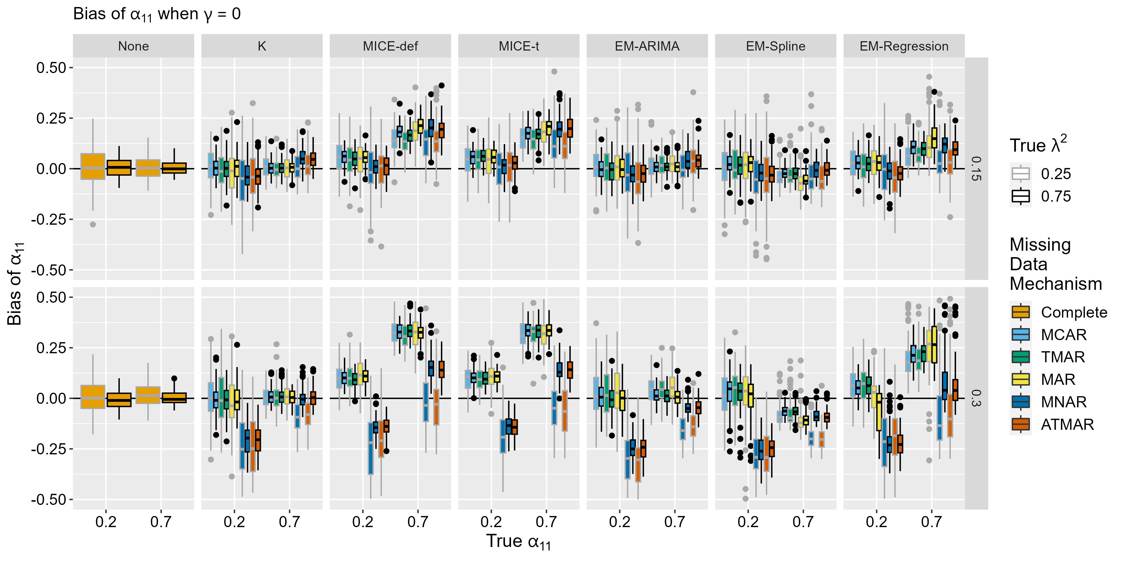
Figure 2: The above graphs shows the bias of the estimated $\alpha$ (on the y-axis) by the true $\alpha$ (on the x-axis for $\gamma$ = 0. The respective missingness mechanisms are shown: complete data (orange), MCAR (sky blue), TMAR (green), MAR (yellow), MNAR (dark blue), and ATMAR (dark orange). The outlines on the box plots show the differing loading conditions: light grey for low loadings/high measurement error and black for high loadings/low measuremenent error. As the y-axis was restricted to range from -.5 to .5, 926 outliers were removed, primarily from the EM-Regression condition. For the box plots, the bottom of the box is the first quartile, the central line is the median, the top of the box is the third quartile, the whiskers extend 1.5(Interquartile Range), and the dots beyond the whiskers are outliers.

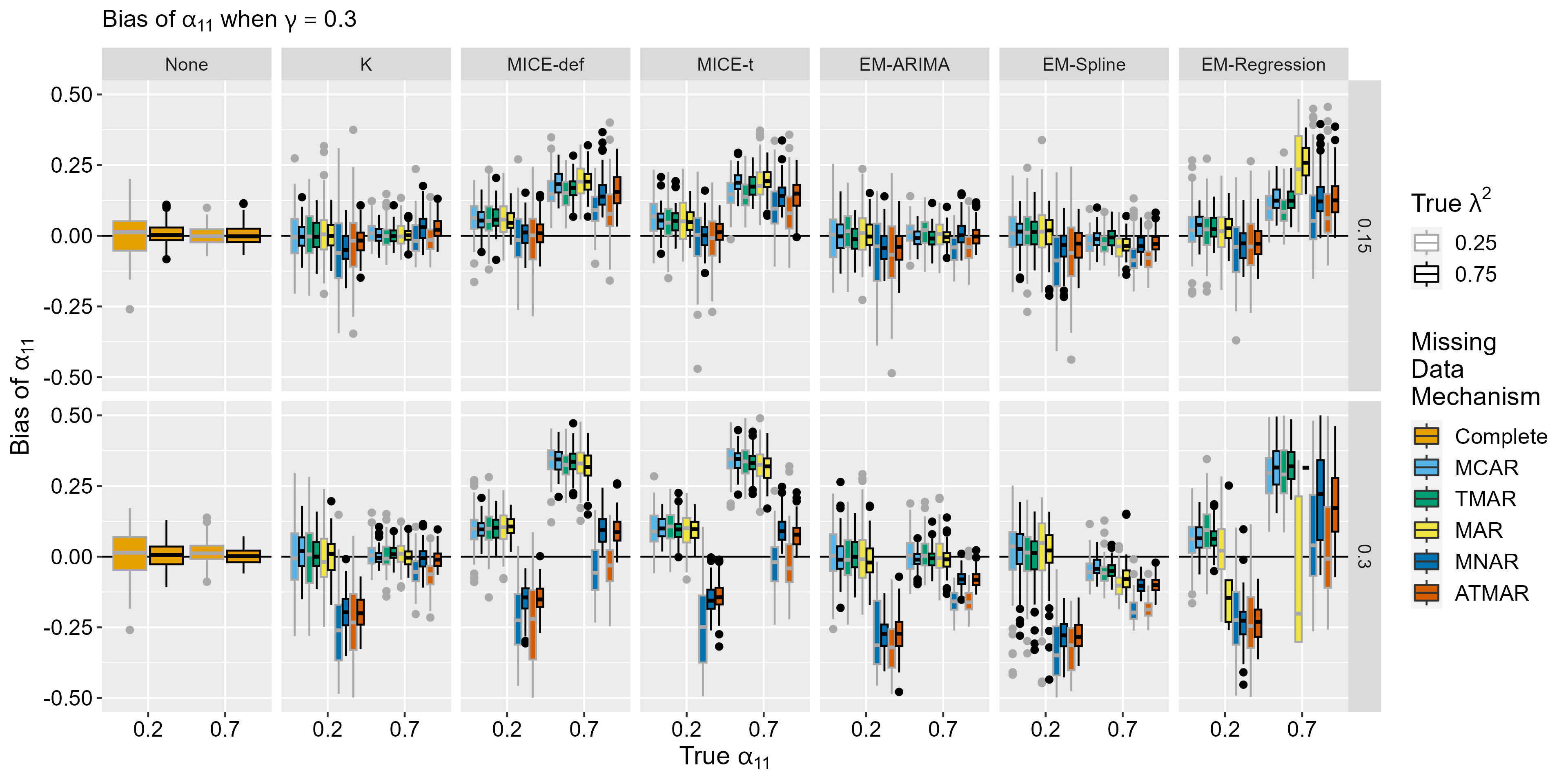
Figure 3: The above graphs shows the bias of the estimated $\alpha$ (on the y-axis) by the true $\alpha$ (on the x-axis for $\gamma$ = .3. The respective missingness mechanisms are shown: complete data (orange), MCAR (sky blue), TMAR (green), MAR (yellow), MNAR (dark blue), and ATMAR (dark orange). The outlines on the box plots show the differing loading conditions: light grey for low loadings/high measurement error and black for high loadings/low measuremenent error. As the y-axis was restricted to range from -.5 to .5, 1171 outliers were removed, primarily from the EM-Regression condition. For the box plots, the bottom of the box is the first quartile, the central line is the median, the top of the box is the third quartile, the whiskers extend 1.5(Interquartile Range), and the dots beyond the whiskers are outliers.

We found that $\alpha_{11}$, the autoregressive parameter associated with missing data, had greater bias than $\alpha_{22}$, the autoregressive parameter associated with complete data, though in Figures 4 and 5 we only include $\alpha_{11}$. These figures show the bias of the $\alpha_{11}$ parameter estimates with respect to $\lambda^{2}$ and missingness mechanisms, for $\gamma$ = 0 and $\gamma$ = .3 respectively. For all graphs, the trend in $\gamma$ was linear (i.e., the relationship between $\gamma$ = 0 and $\gamma$ = .3 is merely a more extreme version of the relationships between $\gamma$ = 0 and $\gamma$ = .15, and $\gamma$ = .15 and $\gamma$ = .3), so, for all of the graphs, we only consider the $\gamma$ = 0 and $\gamma$ = .3 conditions. In Figure 4, we see that there is no effect of $\lambda^{2}$, but bias increases as the true value of the autoregressive effect increases. There is greater bias when increasing the amount of missingness. The Kalman filter is the most successful method for recovering the autoregressive effects, while the multiple imputation methods struggle. Notice that the MCAR graph is similar to the TMAR graph and the MAR graph in that they have less bias and variability than the ATMAR graph which is similar to the the MNAR graph in that they have greater bias and variability. In Figure 5, for the conditions that struggle to recover $\alpha$ (i.e., EM-regression with high autoregressive effects), there is an effect of $\gamma$, otherwise there is not; however, as the strength of the true autoregressive effect increases, the bias increases. With an increase in percent of missingness comes an increase in bias. Again, the Kalman filter succeeds, where the multiple imputation methods fail, and the ATMAR/MNAR data shows greater bias and variability. We do not see an effect of $\gamma$.

3.2 State Cross-Lag Parameter ($\gamma$)

Figure 4: The above graphs shows the bias of the estimated $\gamma$ (on the y-axis) by the true $\gamma$ (on the x-axis for $\alpha$ = .2. The respective missingness mechanisms are shown: complete data (orange), MCAR (sky blue), TMAR (green), MAR (yellow), MNAR (dark blue), and ATMAR (dark orange). The outlines on the box plots show the differing loading conditions: light grey for low loadings/high measurement error and black for high loadings/low measuremenent error. As the y-axis was restricted to range from -.5 to .5, 440 outliers were removed, primarily from the EM-Regression condition. For the box plots, the bottom of the box is the first quartile, the central line is the median, the top of the box is the third quartile, the whiskers extend 1.5(Interquartile Range), and the dots beyond the whiskers are outliers.

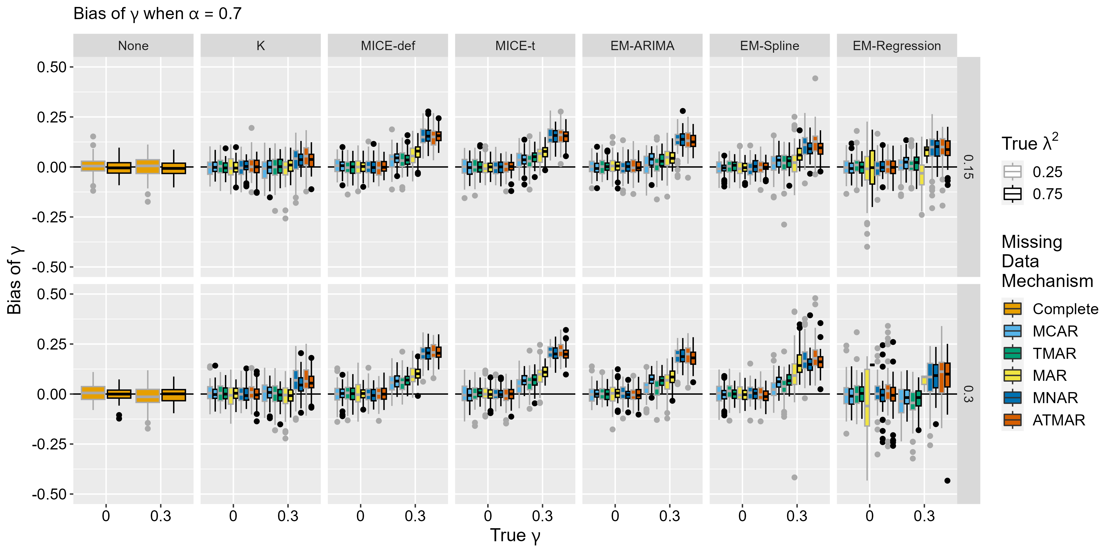
Figure 5: The above graphs shows the bias of the estimated $\gamma$ (on the y-axis) by the true $\gamma$ (on the x-axis for $\alpha$ = .7. The respective missingness mechanisms are shown: complete data (orange), MCAR (sky blue), TMAR (green), MAR (yellow), MNAR (dark blue), and ATMAR (dark orange). The outlines on the box plots show the differing loading conditions: light grey for low loadings/high measurement error and black for high loadings/low measuremenent error. As the y-axis was restricted to range from -.5 to .5, 748 outliers were removed, primarily from the EM-Regression condition. For the box plots, the bottom of the box is the first quartile, the central line is the median, the top of the box is the third quartile, the whiskers extend 1.5(Interquartile Range), and the dots beyond the whiskers are outliers.

We found that $\gamma_{12}$, the cross-lag relation from $X_{1}$ (the variable with missing indicators) to $X_{2}$. had more bias that $\gamma_{21}$, the $\gamma$ associated with complete data (and set to null), though Figures 6 and 7 only depict $\gamma_{12}$. These figures show the bias of the $\gamma_{12}$ parameter with respect to $\lambda^{2}$ and missingness mechanisms for $\alpha$ = .2 and $\alpha$ = .7 respectively. In Figure 6, we see that the bias increases with an increase in the strength of the true $\gamma$ parameter. Increasing the percent missingness increases bias. $\gamma$ is recovered well for MCAR, MAR, and TMAR, but there is more variability and bias in ATMAR and MNAR. Again, we see that the Kalman filter excels at recovering the $\gamma$ parameter, while the MICE conditions struggle. In Figure 7, we see increasing the strength of the true $\gamma$ parameter increases the bias. With an increase in percent missingness, comes an increase in bias. MCAR, MAR, and TMAR are successful at recovering the $\gamma$ parameter, while ATMAR and MNAR show greater bias and variability. Finally, the Kalman filter is again the best method for handling missing data, while MICE-def shows more bias. We do not see an effect of $\alpha$.

3.3 Measurement Loadings and Error ($\lambda^{2}$ and $\sigma^{2}$)

For $\sigma^{2}$, we saw similar bias between $\sigma^{2}_{1}$, $\sigma^{2}_{2}$, and $\sigma^{2}_{3}$, the $\sigma^{2}$s associated with missingness, which was higher than the similar biases $\sigma_{4}$, $\sigma_{5}$, and $\sigma_{6}$, the $\sigma^{2}$s associated with complete data. Due to this similarity, $\sigma^{2}_{1}$, $\sigma^{2}_{2}$, and $\sigma^{2}_{3}$ are treated as one variable in Figures 1 and 2 in the supplementary materials. These graphs show the bias of $\sigma^{2}$ with respect to $\lambda^{2}$ and missingness mechanisms for $\alpha$ = .2 and $\alpha$ = .7 respectively. In Figure 1 in the supplementary materials, there is greater variability with greater measurement error. Increasing percent missingness increases bias. We see lesser bias and variability in MCAR, MAR, and TMAR and greater bias and variability in ATMAR and MNAR. Unlike in the previous cases, the Kalman filter and both MICE conditions can all recover the $\sigma^{2}$ parameters. In Figure 2 in the supplementary materials, again we see that increasing the strength of the measurement error and the percentage of missingness results in greater bias. MCAR, MAR, and TMAR show lesser bias and variability, while ATMAR and MNAR show greater bias and variability. Again, we see the contrary result that, in addition to the Kalman filter and both MICE conditions can recover the $\sigma^{2}$ parameter. For Figures 1 and 2 in the supplementary materials, we do not see an effect of $\alpha$.

For $\lambda^{2}$, we saw similar bias between $\lambda_{11}^{2}$, $\lambda_{12}^{2}$, and $\lambda_{13}^{2}$, the $\lambda^{2}$s associated with missingness, which was higher than the similar biases $\lambda_{24}$, $\lambda_{25}$, and $\sigma_{26}$, the $\sigma^{2}$s associated with complete data. Due to this similarity, $\lambda_{11}^{2}$, $\lambda_{12}^{2}$, and $\lambda_{13}^{2}$ are treated as one variable in Figures 3 and 4 in the supplementary materials . These graphs show the bias of $\lambda^{2}$ with respect to $\gamma$ and missingness mechanisms for $\alpha$ = .2 and $\alpha$ = .7 respectively. In figure 3 in the supplementary materials, we see no effect of $\gamma$, though increasing the strength of the loadings and the percent of missingness results in greater bias. ATMAR and MNAR have greater variability and bias than MCAR, MAR, and TMAR. For the lower bias conditions (i.e., MCAR, MAR and TMAR), the Kalman filter and the MICE conditions recover the loadings successfully, but struggle with MNAR and ATMAR conditons. In Figure 4 in the supplementary materials, we also see increased bias for the $\lambda^{2}$s associated with missingness as compared to the $\lambda^{2}$s associated with complete data. We see no effect of $\gamma$, though increasing the strength of the loadings and the percentage of missingness increases bias. We see the same missingness groupings as MCAR, MAR, and TMAR are associated with lesser bias and variability and ATMAR and MNAR are associated with greater bias and variability. Finally, Kalman filter again recovers the $\lambda^{2}$ parameter, while both MICE conditions fail to successfully recover the $\lambda^{2}$ parameter. Comparing the two graphs, we see an effect of $\alpha$ in that there is greater bias and variability with stronger $\alpha$.

4 Discussion

Overall, we offer the following recommendations for handling missing EMA data in discrete time continuous measure state-space models. The Kalman filter is a good choice for missing data imputation: the approach resulted in the smallest parameter bias no matter the underlying missing data mechanism. With the default settings, multiple imputation methods (i.e., MICE-def and MICE-t) struggle to recover the autoregressive and cross-lagged effects, with bias in parameter recovery particularly high in MNAR and ATMAR settings. Finally, If the missingness is MCAR, MAR, or TMAR as opposed to ATMAR or MNAR, there will be less issues with parameter estimation; though if handled with the Kalman filter, there is little difference between these conditions.

First, it was expected that the bias would be greater for the parameters associated with missingness than the parameters associated with complete data and for stronger true parameters. These former parameters are more impacted by missing observations whereas the latter parameters rely on complete, unaltered information. Thus, we expect to see more bias in these conditions. Second, it also makes sense that as the strength of the parameters increases, the bias increases. However, particularly for the estimates of the autoregressive and cross lagged parameters, larger magnitude effects led to improved performance of the Kalman filtering approach. Third, it is expected that increased missingness results in increased bias. In these conditions, there are simply fewer of the true values, allowing for more opportunities for biased estimates.

Fourth, the Kalman filtering approach performed best out of all the methods. Recall that the Kalman filter estimates the expected values of states using both previous values of states and observed measurements. As such, the Kalman filter (and, also, other filtering methods) explicitly works on the level of unobserved states, while the other imputation methods are all attempting to impute the missing observed variables. This explains the improved performance of the Kalman filter for strong autoregressive and cross-lagged relations. When the states are strongly linked in time, that means your prediction of the states at a timepoint with missing data will be better (because you know that the states are very similar to previous timepoints). An important limitation here is that we knew the true data generating process was a state-space model, which has implications for how the observed data is related to the unobserved states. Given that, it makes sense that the Kalman filter is performing well in this setting, but, for other time series models and in empirical settings, the performance of the Kalman filter will likely be worse than what is observed here.

Fifth, it was a surprise that MICE-def could not recover the autoregressive and cross-lagged parameters, but performed well with the measurement error parameter. Multiple imputation is generally the recommended method for handling missing data (Rubin, 1996), so it is unexpected that it performed poorly. Furthermore, we used the default settings in the functions as we expect most users to do the same. Because of the general performance of multiple imputation with the default settings, we do not recommend using these packages for imputation with the default settings. Even so, recall what MICE-def does: it is a cross-sectional method which builds the imputation model without considering temporal relations. Hence, it makes sense that it can recover the measurement error (as this is purely cross-sectional), but struggles with recovering the dynamics. In an attempt to resolve this issue, the MICE-t condition did take into account the temporal relations in the data with a lag-1 matrix serving as the predictor in the imputation model. Even with this alteration, MICE-t struggled in ways similarly to MICE-def. We hypothesize that, though MICE-t does take into account the time dependence, it still performs less well than the Kalman filter because it cannot take into account information from the latent states.

Sixth, the EM algorithms, particularly EM-ARIMA and EM-Spline performed well with lower levels of missing data (i.e., 15% missingness), though struggled with higher levels of missingness (i.e., 30% missingness). EM-Regression generally performed poorly, and, from many of the analyses for this method, we had to remove outliers. Because the success of the EM-Regression method depends on the predictive relationship between $y_{4}$-$y_{6}$ and $y_{1}$-$y_{3}$, and given that this varies with $\gamma$ (in that low values of $\gamma$ would correspond to less predictive power), it makes sense that this method struggled. In addition, the EM algorithm is an algorithm for obtaining maximum likelihood estimates, and it is well-established that using these estimates to generate imputations has numerous shortcomings (Gómez-Carracedo ., 2014). Such a method amounts to regression imputation (in that the expectation step is simply the results of predictions from a series of regression equations), resulting in restricted variation, biased associations, among other problems (Gómez-Carracedo ., 2014). Despite EM-ARIMA and EM-Spline performing well at lower levels of missingness, using maximum likelihood estimation followed by single imputation is not recommended as a missing data solution.

Finally, we see a division between MCAR/MAR/TMAR and ATMAR/MNAR. Recall that MCAR and TMAR are both missing data mechanisms that do not rely on other variables in the model for their missingness. Hence, it is expected that they would perform similarly. However, we reiterate the warning that most if not all missing data will not be MCAR (and will rarely be purely TMAR). Additionally, MNAR and ATMAR performed approximately the same (notably with Kalman filtering resulting in the lowest bias). This is likely because MNAR and ATMAR are two aspects of the same type of missingness mechanisms. Where MNAR is missingness based on the missing variables value, ATMAR is missingness based on a previous timepoint’s value (which may or may not be missing). This results in a danger, as not taking into account temporal dependency might result in reduced model performance, and an opportunity, as temporal dependency offers more information to impute missing values from. Further research on missingness mechanisms and how they unfold across time should be pursued.

The reader may having the following concerns about this project: the use of default methods for MICE-def, no varying of states and indicators or number of time points, and what if the phenomenon is continuous. First, we used the default settings for MICE-def as this will be the most common choice by users of the software, and that the default settings (with use predictive mean matching) have been shown to be effective across a number of settings. Due to the lack of success with MICE-def, we followed up with MICE-t, the time-dependent imputation mode, and found that, even with improvements to MICE, the method was unable to recover the time-series parameters that were dependent on states. Second, we did not increase the number of states or indicators, as we expect the bias and issues to increase with an increasing number of states, and we expect the measurement to improve with an increasing number of indicators (which will likely result in lower bias, but not necessarily for the multiple imputation methods). Third, we evaluated only one sample size (500 time points) as we assume that any bias due to missingness will be exacerbated with smaller numbers of time points. Fourth, there are limits to imputation. If you are modeling a continuous process as discrete, you are missing all of the infinitesimal points between the discrete time points. There are limits to how much missing data can be handled by an imputation method (see below), and this would be a case where it would be best to just use a continuous time model.

For future directions, first, we would like to further evaluate the use of multiple imputation methods for time series and state-space data as this analysis relied on the default setting and, also, include Amelia in our analyses. These methods are flexible, which implies that, with different base modeling choices, we could theoretically improve performance. However, this would be specific to different datasets and models. Second, it is often recommended that the way to handle missing data in a state-space model is to fit a continuous time model. As a next step, we will compare the best discrete time missing data method, the Kalman filter, to a continuous time model. For a continuous time model, a Kalman-Bucy filter is used which discretizes the continuous time into small intervals (Kálmán  Bucy, 1961). If the underlying process is discrete, then this would simplify into the Kalman. However, if it is not, we expect to see differences in the discrete and continuous time models. Finally, we see that the Kalman filter is successful at 30%, but we are interested to see what the limit for amount of missingness is for the Kalman filter in order to provide better recommendations. Thus, we will be testing increasing amounts of missingness to see when the Kalman filter fails.

References

- Bannon Jr. (\APACyear2015) \APACinsertmetastarbannon_jr_missing_2015{APACrefauthors}Bannon Jr., W. \APACrefYearMonthDay2015. \BBOQ\APACrefatitleMissing data within a quantitative research study: How to assess it, treat it, and why you should care Missing data within a quantitative research study: How to assess it, treat it, and why you should care.\BBCQ \APACjournalVolNumPagesJournal of the American Association of Nurse Practitioners274230–232. \APACrefnotePublisher: John Wiley & Sons, Ltd {APACrefDOI} 10.1002/2327-6924.12208 \PrintBackRefs\CurrentBib
- Beck \BOthers. (\APACyear1961) \APACinsertmetastarbeck_inventory_1961{APACrefauthors}Beck, A\BPBIT., Ward, C\BPBIH., Mendelson, M., Mock, J.\BCBL \BBA Erbaugh, J. \APACrefYearMonthDay1961. \BBOQ\APACrefatitleAn Inventory for Measuring Depression An Inventory for Measuring Depression.\BBCQ \APACjournalVolNumPagesArchives of General Psychiatry46561–571. {APACrefDOI} 10.1001/archpsyc.1961.01710120031004 \PrintBackRefs\CurrentBib
- Bhaskaran \BBA Smeeth (\APACyear2014) \APACinsertmetastarbhaskaran_what_2014{APACrefauthors}Bhaskaran, K.\BCBT \BBA Smeeth, L. \APACrefYearMonthDay2014. \BBOQ\APACrefatitleWhat is the difference between missing completely at random and missing at random? What is the difference between missing completely at random and missing at random?\BBCQ \APACjournalVolNumPagesInternational Journal of Epidemiology4341336–1339. {APACrefDOI} 10.1093/ije/dyu080 \PrintBackRefs\CurrentBib
- Dempster \BOthers. (\APACyear1977) \APACinsertmetastardempster_maximum_1977{APACrefauthors}Dempster, A\BPBIP., Laird, N\BPBIM.\BCBL \BBA Rubin, D\BPBIB. \APACrefYearMonthDay1977. \BBOQ\APACrefatitleMaximum Likelihood from Incomplete Data via the EM Algorithm Maximum Likelihood from Incomplete Data via the EM Algorithm.\BBCQ \APACjournalVolNumPagesJournal of the Royal Statistical Society. Series B (Methodological)3911–38. \APACrefnotePublisher: [Royal Statistical Society, Wiley] \PrintBackRefs\CurrentBib
- Donders \BOthers. (\APACyear2006) \APACinsertmetastardonders_review_2006{APACrefauthors}Donders, A\BPBIR\BPBIT., van der Heijden, G\BPBIJ., Stijnen, T.\BCBL \BBA Moons, K\BPBIG. \APACrefYearMonthDay2006\APACmonth10. \BBOQ\APACrefatitleReview: A gentle introduction to imputation of missing values Review: A gentle introduction to imputation of missing values.\BBCQ \APACjournalVolNumPagesJournal of Clinical Epidemiology59101087–1091. {APACrefURL} https://www.sciencedirect.com/science/article/pii/S0895435606001971 {APACrefDOI} 10.1016/j.jclinepi.2006.01.014 \PrintBackRefs\CurrentBib
- El-Masri \BBA Fox-Wasylyshyn (\APACyear2005) \APACinsertmetastarel-masri_missing_2005{APACrefauthors}El-Masri, M\BPBIM.\BCBT \BBA Fox-Wasylyshyn, S\BPBIM. \APACrefYearMonthDay2005. \BBOQ\APACrefatitleMissing Data: An Introductory Conceptual Overview for the Novice Researcher. Missing Data: An Introductory Conceptual Overview for the Novice Researcher.\BBCQ \APACjournalVolNumPagesCJNR: Canadian Journal of Nursing Research374156–171. \APACrefnotePlace: Canada Publisher: McGill University/School of Nursing \PrintBackRefs\CurrentBib
- Gómez-Carracedo \BOthers. (\APACyear2014) \APACinsertmetastargomez-carracedo_practical_2014{APACrefauthors}Gómez-Carracedo, M., Andrade, J., López-Mahía, P., Muniategui, S.\BCBL \BBA Prada, D. \APACrefYearMonthDay2014\APACmonth05. \BBOQ\APACrefatitleA practical comparison of single and multiple imputation methods to handle complex missing data in air quality datasets A practical comparison of single and multiple imputation methods to handle complex missing data in air quality datasets.\BBCQ \APACjournalVolNumPagesChemometrics and Intelligent Laboratory Systems13423–33. {APACrefURL} https://www.sciencedirect.com/science/article/pii/S016974391400032X {APACrefDOI} 10.1016/j.chemolab.2014.02.007 \PrintBackRefs\CurrentBib
- Hardt \BOthers. (\APACyear2013) \APACinsertmetastarhardt_multiple_2013{APACrefauthors}Hardt, J., Herke, M., Brian, T.\BCBL \BBA Laubach, W. \APACrefYearMonthDay2013. \BBOQ\APACrefatitleMultiple Imputation of Missing Data: A Simulation Study on a Binary Response Multiple Imputation of Missing Data: A Simulation Study on a Binary Response.\BBCQ \APACjournalVolNumPagesOpen Journal of Statistics03370–378. {APACrefDOI} 10.4236/ojs.2013.35043 \PrintBackRefs\CurrentBib
- Honaker \BOthers. (\APACyear2011) \APACinsertmetastarhonaker_amelia_2011{APACrefauthors}Honaker, J., King, G.\BCBL \BBA Blackwell, M. \APACrefYearMonthDay2011. \BBOQ\APACrefatitleAmelia II: A Program for Missing Data Amelia II: A Program for Missing Data.\BBCQ \APACjournalVolNumPagesJournal of Statistical Software4571 – 47. \APACrefnoteSection: Articles {APACrefDOI} 10.18637/jss.v045.i07 \PrintBackRefs\CurrentBib
- Ji \BOthers. (\APACyear2018) \APACinsertmetastarji_handling_2018{APACrefauthors}Ji, L., Chow, S\BHBIM., Schermerhorn, A., Jacobson, N.\BCBL \BBA Cummings, E. \APACrefYearMonthDay2018. \BBOQ\APACrefatitleHandling Missing Data in the Modeling of Intensive Longitudinal Data Handling Missing Data in the Modeling of Intensive Longitudinal Data.\BBCQ \APACjournalVolNumPagesStructural Equation Modeling25. {APACrefDOI} 10.1080/10705511.2017.1417046 \PrintBackRefs\CurrentBib
- Junger \BBA Ponce de Leon (\APACyear2015) \APACinsertmetastarjunger_imputation_2015{APACrefauthors}Junger, W.\BCBT \BBA Ponce de Leon, A. \APACrefYearMonthDay2015. \BBOQ\APACrefatitleImputation of missing data in time series for air pollutants Imputation of missing data in time series for air pollutants.\BBCQ \APACjournalVolNumPagesAtmospheric Environment10296–104. {APACrefDOI} 10.1016/j.atmosenv.2014.11.049 \PrintBackRefs\CurrentBib
- Kálmán \BBA Bucy (\APACyear1961) \APACinsertmetastarKlmn1961NewRI{APACrefauthors}Kálmán, R\BPBIE.\BCBT \BBA Bucy, R\BPBIS. \APACrefYearMonthDay1961. \BBOQ\APACrefatitleNew Results in Linear Filtering and Prediction Theory New results in linear filtering and prediction theory.\BBCQ \APACjournalVolNumPagesJournal of Basic Engineering8395-108. {APACrefURL} https://api.semanticscholar.org/CorpusID:8141345 \PrintBackRefs\CurrentBib
- R\BPBIJ\BPBIA. Little (\APACyear1988) \APACinsertmetastarlittle_test_1988{APACrefauthors}Little, R\BPBIJ\BPBIA. \APACrefYearMonthDay1988. \BBOQ\APACrefatitleA Test of Missing Completely at Random for Multivariate Data with Missing Values A Test of Missing Completely at Random for Multivariate Data with Missing Values.\BBCQ \APACjournalVolNumPagesJournal of the American Statistical Association834041198–1202. \APACrefnotePublisher: Taylor & Francis {APACrefDOI} 10.1080/01621459.1988.10478722 \PrintBackRefs\CurrentBib
- T\BPBID. Little \BOthers. (\APACyear2014) \APACinsertmetastarlittle_joys_2014{APACrefauthors}Little, T\BPBID., Jorgensen, T\BPBID., Lang, K\BPBIM.\BCBL \BBA Moore, E\BPBIW\BPBIG. \APACrefYearMonthDay2014. \BBOQ\APACrefatitleOn the Joys of Missing Data On the Joys of Missing Data.\BBCQ \APACjournalVolNumPagesJournal of Pediatric Psychology392151–162. {APACrefDOI} 10.1093/jpepsy/jst048 \PrintBackRefs\CurrentBib
- Martino \BOthers. (\APACyear2018) \APACinsertmetastarmartino_assessment_2018{APACrefauthors}Martino, I., Santangelo, G., Moschella, D., Marino, L., Servidio, R., Augimeri, A.\BDBLCerasa, A. \APACrefYearMonthDay2018. \BBOQ\APACrefatitleAssessment of Snaith-Hamilton Pleasure Scale (SHAPS): the dimension of anhedonia in Italian healthy sample Assessment of Snaith-Hamilton Pleasure Scale (SHAPS): the dimension of anhedonia in Italian healthy sample.\BBCQ \APACjournalVolNumPagesNeurological Sciences394657–661. {APACrefDOI} 10.1007/s10072-018-3260-2 \PrintBackRefs\CurrentBib
- McKee \BOthers. (\APACyear2020) \APACinsertmetastarmckee_emotion_2020{APACrefauthors}McKee, K., Russell, M., Mennis, J., Mason, M.\BCBL \BBA Neale, M. \APACrefYearMonthDay2020. \BBOQ\APACrefatitleEmotion regulation dynamics predict substance use in high-risk adolescents Emotion regulation dynamics predict substance use in high-risk adolescents.\BBCQ \APACjournalVolNumPagesAddictive Behaviors106106374. {APACrefDOI} https://doi.org/10.1016/j.addbeh.2020.106374 \PrintBackRefs\CurrentBib
- Newman (\APACyear2014) \APACinsertmetastarnewman_missing_2014{APACrefauthors}Newman, D\BPBIA. \APACrefYearMonthDay2014. \BBOQ\APACrefatitleMissing Data: Five Practical Guidelines Missing Data: Five Practical Guidelines.\BBCQ \APACjournalVolNumPagesOrganizational Research Methods174372–411. \APACrefnotePublisher: SAGE Publications Inc {APACrefDOI} 10.1177/1094428114548590 \PrintBackRefs\CurrentBib
- Petris (\APACyear2010) \APACinsertmetastarpetris_r_2010{APACrefauthors}Petris, G. \APACrefYearMonthDay2010. \BBOQ\APACrefatitleAn R Package for Dynamic Linear Models An R Package for Dynamic Linear Models.\BBCQ \APACjournalVolNumPagesJournal of Statistical Software36121 – 16. \APACrefnoteSection: Articles {APACrefDOI} 10.18637/jss.v036.i12 \PrintBackRefs\CurrentBib
- Plumpton \BOthers. (\APACyear2016) \APACinsertmetastarplumpton_multiple_2016{APACrefauthors}Plumpton, C\BPBIO., Morris, T., Hughes, D\BPBIA.\BCBL \BBA White, I\BPBIR. \APACrefYearMonthDay2016. \BBOQ\APACrefatitleMultiple imputation of multiple multi-item scales when a full imputation model is infeasible Multiple imputation of multiple multi-item scales when a full imputation model is infeasible.\BBCQ \APACjournalVolNumPagesBMC Research Notes9145. {APACrefDOI} 10.1186/s13104-016-1853-5 \PrintBackRefs\CurrentBib
- Rubin (\APACyear1976) \APACinsertmetastarrubin_inference_1976{APACrefauthors}Rubin, D\BPBIB. \APACrefYearMonthDay1976. \BBOQ\APACrefatitleInference and Missing Data Inference and Missing Data.\BBCQ \APACjournalVolNumPagesBiometrika633581–592. \APACrefnotePublisher: [Oxford University Press, Biometrika Trust] {APACrefDOI} 10.2307/2335739 \PrintBackRefs\CurrentBib
- Rubin (\APACyear1996) \APACinsertmetastarrubin_multiple_1996{APACrefauthors}Rubin, D\BPBIB. \APACrefYearMonthDay1996. \BBOQ\APACrefatitleMultiple Imputation After 18+ Years Multiple Imputation After 18+ Years.\BBCQ \APACjournalVolNumPagesJournal of the American Statistical Association91434473–489. \APACrefnotePublisher: [American Statistical Association, Taylor & Francis, Ltd.] {APACrefDOI} 10.2307/2291635 \PrintBackRefs\CurrentBib
- Rubin \BBA Schenker (\APACyear1986) \APACinsertmetastarrubin_multiple_1986{APACrefauthors}Rubin, D\BPBIB.\BCBT \BBA Schenker, N. \APACrefYearMonthDay1986. \BBOQ\APACrefatitleMultiple Imputation for Interval Estimation From Simple Random Samples With Ignorable Nonresponse Multiple Imputation for Interval Estimation From Simple Random Samples With Ignorable Nonresponse.\BBCQ \APACjournalVolNumPagesJournal of the American Statistical Association81394366–374. \APACrefnotePublisher: [American Statistical Association, Taylor & Francis, Ltd.] {APACrefDOI} 10.2307/2289225 \PrintBackRefs\CurrentBib
- Shiffman \BOthers. (\APACyear2008) \APACinsertmetastarshiffman_ecological_2008{APACrefauthors}Shiffman, S., Stone, A\BPBIA.\BCBL \BBA Hufford, M\BPBIR. \APACrefYearMonthDay2008. \BBOQ\APACrefatitleEcological Momentary Assessment Ecological Momentary Assessment.\BBCQ \APACjournalVolNumPagesAnnual Review of Clinical Psychology411–32. \APACrefnotePublisher: Annual Reviews {APACrefDOI} 10.1146/annurev.clinpsy.3.022806.091415 \PrintBackRefs\CurrentBib
- Sinharay \BOthers. (\APACyear2001) \APACinsertmetastarsinharay_use_2001{APACrefauthors}Sinharay, S., Stern, H\BPBIS.\BCBL \BBA Russell, D. \APACrefYearMonthDay2001. \BBOQ\APACrefatitleThe use of multiple imputation for the analysis of missing data. The use of multiple imputation for the analysis of missing data.\BBCQ \APACjournalVolNumPagesPsychological Methods6317–329. \APACrefnotePlace: US Publisher: American Psychological Association {APACrefDOI} 10.1037/1082-989X.6.4.317 \PrintBackRefs\CurrentBib
- Snaith \BOthers. (\APACyear1995) \APACinsertmetastarsnaith_scale_1995{APACrefauthors}Snaith, R\BPBIP., Hamilton, M., Morley, S., Humayan, A., Hargreaves, D.\BCBL \BBA Trigwell, P. \APACrefYearMonthDay1995. \BBOQ\APACrefatitleA Scale for the Assessment of Hedonic Tone the Snaith–Hamilton Pleasure Scale A Scale for the Assessment of Hedonic Tone the Snaith–Hamilton Pleasure Scale.\BBCQ \APACjournalVolNumPagesBritish Journal of Psychiatry167199–103. \APACrefnoteEdition: 2018/01/02 Publisher: Cambridge University Press {APACrefDOI} 10.1192/bjp.167.1.99 \PrintBackRefs\CurrentBib
- Trevor Hastie \BBA Robert Tibshirani (\APACyear1986) \APACinsertmetastartrevor_hastie_generalized_1986{APACrefauthors}Trevor Hastie\BCBT \BBA Robert Tibshirani. \APACrefYearMonthDay1986. \BBOQ\APACrefatitleGeneralized Additive Models Generalized Additive Models.\BBCQ \APACjournalVolNumPagesStatistical Science13297–310. {APACrefDOI} 10.1214/ss/1177013604 \PrintBackRefs\CurrentBib
- van Buuren \BBA Groothuis-Oudshoorn (\APACyear2011) \APACinsertmetastarvan_Buuren_2011{APACrefauthors}van Buuren, S.\BCBT \BBA Groothuis-Oudshoorn, K. \APACrefYearMonthDay2011. \BBOQ\APACrefatitlemice: Multivariate Imputation by Chained Equations in R mice: Multivariate imputation by chained equations in r.\BBCQ \APACjournalVolNumPagesJournal of Statistical Software4531-67. {APACrefDOI} 10.18637/jss.v045.i03 \PrintBackRefs\CurrentBib
- van Buuren \BBA Groothuis-Oudshoorn (\APACyear2011) \APACinsertmetastarvan_buuren_mice_2011{APACrefauthors}van Buuren, S.\BCBT \BBA Groothuis-Oudshoorn, K. \APACrefYearMonthDay2011. \BBOQ\APACrefatitlemice: Multivariate Imputation by Chained Equations in R mice: Multivariate Imputation by Chained Equations in R.\BBCQ \APACjournalVolNumPagesJournal of Statistical Software4531 – 67. \APACrefnoteSection: Articles {APACrefDOI} 10.18637/jss.v045.i03 \PrintBackRefs\CurrentBib
- Zaninotto \BBA Sacker (\APACyear2017) \APACinsertmetastarzaninotto_missing_2017{APACrefauthors}Zaninotto, P.\BCBT \BBA Sacker, A. \APACrefYearMonthDay2017. \BBOQ\APACrefatitleMissing Data in Longitudinal Surveys: A Comparison of Performance of Modern Techniques Missing Data in Longitudinal Surveys: A Comparison of Performance of Modern Techniques.\BBCQ \APACjournalVolNumPagesJournal of Modern Applied Statistical Methods16378–402. {APACrefDOI} 10.22237/jmasm/1509495600 \PrintBackRefs\CurrentBib