Efficient cooling of high-angular-momentum atoms

Abstract

We propose a highly efficient and fast method of translational cooling for high-angular-momentum atoms. Optical pumping and stimulated transitions, combined with magnetic forces, can be used to compress phase-space density, and the efficiency of each compression step increases with the angular momentum. Entropy is removed by spontaneously emitted photons, and particle number is conserved. This method may be an attractive alternative to evaporative cooling of atoms and possibly molecules in order to produce quantum degenerate gases.

Keywords: atomic physics, cold atoms, phase-space compression

1 Introduction

Laser cooling, first proposed almost half a century ago, remains the standard approach for producing ultracold atoms [1, 2]. This method relies on momentum transfer from light to atoms as photons are repeatedly scattered, enabling the production and study of ultracold atomic gases. Many improvements on basic laser cooling have advanced the state of the art, including sub-Doppler Sisyphus cooling [3, 4, 5, 6, 7], and sub-recoil degenerate Raman sideband cooling cooling [8, 9].

While laser cooling works extremely well, the requirement of a closed, two-level transition has limited the applicability of the method to a subset of elements in the periodic table. For those atoms, after many years of refinement, laser cooling has reached saturation in its performance due to multiple scattering of resonant photons which create an effective repulsive interaction between the atoms, pushing them apart. An important figure-of-merit is the phase-space density, a dimensionless parameter which is the product of number density and the third power of the average de Broglie wavelength. Laser cooling typically produces a phase-space density of 10^-6. This is also the starting point for creating quantum degenerate gasses with order-unity phase-space density through evaporative cooling in a trap [10, 11], and the creation of the so-called atom laser [12, 13, 14]. Evaporative cooling is even more restrictive than laser cooling, as it relies on elastic collisions between atoms to maintain thermal equilibrium as the hottest atoms are ejected. Inelastic channels create unwanted losses and often make evaporative cooling impossible. Even when working optimally, evaporative cooling is a slow process and results in a significant loss of atom number.

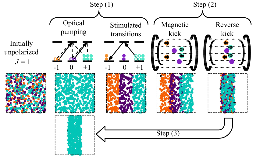
Figure 1: A schematic depiction of the MOP-cooling sequence for ensembles with angular momentum $J=1$. The colored circles represent atoms, initially trapped in a flat, hard-wall potential. The colors represent the atom’s magnetic state (orange: $m_{J}=-1$, purple: $m_{J}=0$, teal: $m_{J}=+1$). A cycle begins with optically pumping all atoms to the same state. Then, a sequence of stimulated transitions correlate the magnetic states with position along the direction of compression. A sequence of one-dimensional magnetic kicks pushes atoms of oppositely-signed magnetic states together. The cycle is closed by optically pumping the compressed atoms back into the same magnetic state. A cycle’s compression factor increases with the number of available magnetic states.

In recent years, alternative approaches to producing cold atoms and molecules were developed (see [15] and references therein). The starting point for much of this work is a supersonic molecular beam where desired atoms or molecules can be entrained in the flow and stopped in a series of pulsed magnetic or electric fields. Alternatively, cold atoms and molecules are produced by buffer-gas cooling [16]. After stopping, these atoms and molecules can be trapped, typically in a magnetic field configuration that confines the low-field seekers to the center of the trap. In parallel, cooling of atoms with a one-way wall was proposed and demonstrated [17, 18, 19], and relies on photon entropy, not momentum as in laser cooling. The one-way wall is the first practical realization of Maxwell’s demon for an ensemble of atoms. While one-way-wall cooling demonstrated a large increase in phase-space density, it did not conserve atom number. To address this limitation, we proposed [20] a variation which we called magneto-optical (MOP) cooling, relying on cycles of state preparation and magnetic kicks.

In this paper, we present a generalized and highly efficient version of MOP cooling that can work for high-angular-momentum atoms and offers an attractive alternative to laser cooling and evaporative cooling. Quantum gases of atoms with high angular momentum have become of increasing scientific interest over the last 20 years [21] making our method timely and relevant to a growing community. As depicted schematically in Fig. 1, and described in detail below, the larger internal-state space of high-angular-momentum atoms may be leveraged to yield a greater compression of an ensemble in real space. This is in contrast to our original proposal [20] that focused on spin-1/2 systems. Our method will help bridge the existing gap of approximately six orders of magnitude between the phase-space density limits of standard sub-Doppler cooling and evaporative cooling, thereby promising larger ultracold samples.

In the following section, our simulation methodology is described, followed by a brief review of MOP cooling for a spin-1/2 system. Then MOP cooling is generalized for high-angular-momentum atoms. We conclude the paper with a discussion of possible limitations to our new method, how those limitations may be overcome, and the significance of MOP cooling in the atomic physics toolbox. The subsequent appendix presents a one-dimensional model of MOP cooling as an alternative to the detailed simulations that follow.

2 MOP cooling

MOP cooling is a conceptually new method that does not rely on the momentum of the photon, making it completely different from laser cooling. The key benefit of this approach is its universality and simplicity, since it relies only on internal magnetic state preparation and magnetic forces from pulsed coils. MOP cooling may be interpreted as a technique that transforms the cooling of internal degrees of freedom via optical pumping [22] to external degrees of freedom. Through numeric simulations, we will evaluate the efficacy of MOP cooling for atoms with different numbers of internal states.

Our MOP-cooling simulations track the three-dimensional positions ${\bf x}$, velocities ${\bf v}$, and magnetic states $m_{J}\in\{-2J,-2J+1,\ldots,2J\}$ of a sample of $N=10^{5}$ atoms, each with total angular-momentum quantum number $J$. The internal magnetic state of each atom is initialized in accordance with the MOP-cooling cycle (discussed further below). Positions are initialized from a flat distribution of a 0.5 cm width. Velocities are initialized from the Maxwell-Boltzmann distribution corresponding to a temperature of $25\times T_{\rm rec}$ where $T_{\rm rec}=h^{2}/Mk_{\rm B}\lambda^{2}$ is the recoil temperature imposed by, e.g., a magneto-optical trap operating at wavelength $\lambda$ to trap a species of mass $M$. Here, $h$ is Planck’s constant and $k_{\rm B}$ is Boltzmann’s constant.

A fourth-order Runge-Kutta algorithm updates the position and velocity of each atom subject to the force ${\bf F}(t)=-m_{J}g_{J}\mu_{\rm B}\nabla\left|{\bf B}({\bf x},t)\right|$ where $g_{J}$ is the Landé $g$-factor of the atom’s ground state, $\mu_{\rm B}$ is the Bohr magneton, and ${\bf B}$ is the pulsed magnetic field arranged to provide the one-dimensional kick. The simulation time step is one microsecond. Table 1 reports the atomic properties used in this study.

Table 1: Atomic properties used for simulation purposes. The Ref. column provides an example of magneto-optical trap operation for each species with a corresponding recoil temperature $T_{\rm rec}$. Values for $g_{J}$ are provided in [23], except for Li for which we adopt the electron’s value.

Atom	$M$	$J$	$g_{J}$	$T_{\rm rec}$	Ref.
	($10^{-26}$ kg)			$({\rm\upmu K})$
Li	$1.15$	1/2	$2.002\,32$	$6.1$	[24]
Cr	$8.63$	3	$2.001\,83$	$2.0$	[25]
Er	$27.83$	6	$1.163\,81$	$0.3$	[26]
Dy	$26.98$	8	$1.241\,59$	$0.3$	[27]

The magnetic field is modeled as two sets of coaxial coil pairs, one in the Maxwell configuration to provide a strong gradient [28] and the other in the Helmholtz configuration to shift the zero-crossing of the field away from the ensemble’s center, thereby providing a nearly-one-dimensional kick. We use superposition of the exact solution for a current-carrying loop to model the full coil geometry. ${\bf B}$ is evaluated on a dense grid for unit current. Vector interpolation allows us to evaluate $\nabla\left|{\bf B}({\bf x})\right|$ at arbitrary positions. Time-dependent current pulses are modeled by scaling the field gradient interpolation result by $I(t)=I_{0}\sin[\pi(t-t_{0})/\tau]$ for $t\in[t_{0},t_{0}+\tau]$ and $I(t)=0$ otherwise, where $I_{0}$ is the peak current, $t_{0}$ is the pulse delay, and $\tau$ is the pulse width. In this paper, we set $\tau=300~{}{\rm\upmu s}$.

The simulated coil parameters are as follows. There are 7 turns $\times$ 2 layers, or 14 loops per Helmholtz coil, each with a nominal radius of $R_{\rm HH}=3.5\,\rm{cm}$, axially-separated by $R_{\rm HH}$, and carrying identically-oriented currents . There are 5 turns $\times$ 2 layers, or 10 loops per Maxwell coil, each with a nominal radius of $R_{\rm HH}/\sqrt{3}$, separated by $R_{\rm HH}$, and carrying oppositely-oriented currents. The peak currents are $I_{0,{\rm HH}}=1000$ A for the Helmholtz coils and $I_{0,{\rm M}}=800$ A for the Maxwell coils. The shared midpoint between the coil pairs is displaced by 0.2 cm in the positive $z$-direction from the initial center of mass of the atomic sample (taken as the origin of the coordinate system). We find that this region provides a more uniform and one-dimensional kick. With these coil parameters, the peak field gradients are approximately 1520 G/cm along the kick direction and 45 G/cm in the transverse directions. Two-dimensional slices of the magnetic field gradient used in our simulations are shown in Figure 2.

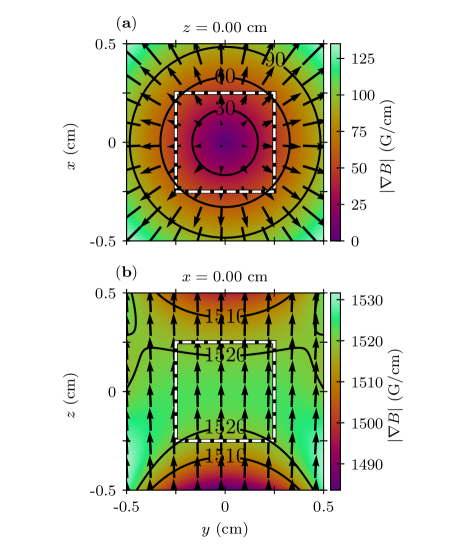
Figure 2: Two-dimensional slices of the magnetic field gradient used for MOP cooling simulations, evaluated at peak current, and shown (a) transverse-to and (b) along the kicking direction. The black-and-white dashed line marks the initial extent of the atomic cloud. The magnitude of the total field $|{\bf B}|$ varies primarily along $z$ in a nearly-linear fashion.

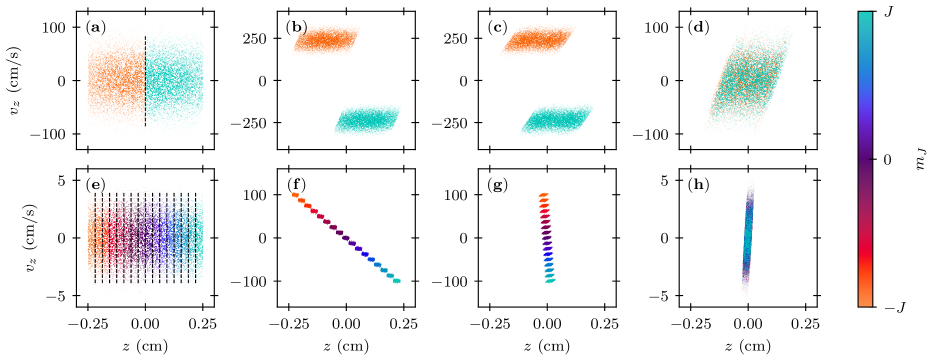
Figure 3: MOP cooling simulations for Li (a-d) and Dy (e-h) visualized in phase-space. Each column of plots represents a snapshot during the magnetic kicks required for a cycle. Initially, the magnetic states are correlated with position along the $z$-axis through optical pumping followed by spatially-resolved coherent population transfer via stimulated transitions. The vertical dashed black lines in panels (a) and (e) mark the ideal boundary between different magnetic states. In panels (b) and (f), a one-dimensional magnetic kick accelerates atoms to a velocity that is proportional to their magnetic state. After waiting an optimized delay time the phase-space distribution has been compressed in real space but remains extended in velocity space, as shown in panels (c) and (g). In panels (d) and (f), we show a reverse kick returning the atom’s velocity distribution to near its original extent while preserving the spatial compression. More precisely, we find the relative difference between standard deviations of the ensembles’ initial and final velocity distribution is below 0.2% for all coordinates and all four species simulated.

For a specific example, consider atomic lithium (Li) trapped using standard techniques [24]. At sufficient magnetic fields, the electronic spin decouples from the nuclear spin yielding a total angular momentum of $J=1/2$; the two electronic $m_{J}$ states are denoted $\left|1/2\right\rangle$ and $\left|-1/2\right\rangle$ and it is in this high-field regime that Li may be MOP-cooled as originally discussed in [20]. The cooling sequence starts with suddenly turning off the trap so that the atoms are free. In step (1) of MOP cooling, all of the atoms are optically pumped to the $\left|1/2\right\rangle$ state. Then, half of the cloud is transferred to the $\left|-1/2\right\rangle$ state by stimulated transitions, i.e., stimulated Raman adiabatic passage (STIRAP) sequences [29, 30], thereby creating two spatially-distinct populations [see Fig. 3 (a)]. In step (2), a magnetic-field-gradient kick is applied to the cloud, thereby causing the two halves to merge [Fig. 3 (b-c)], and then a reverse kick returns the atoms to their original velocity distribution [Fig. 3 (d)]. As demonstrated experimentally in [31], such magnetic kicks can be applied along a single axis while minimally affecting the other two dimensions. In step (3), all atoms are optically-pumped back to the $\left|1/2\right\rangle$ state, thereby completing the cooling cycle. In principle, a factor of $2\times$ in phase-space compression is possible.

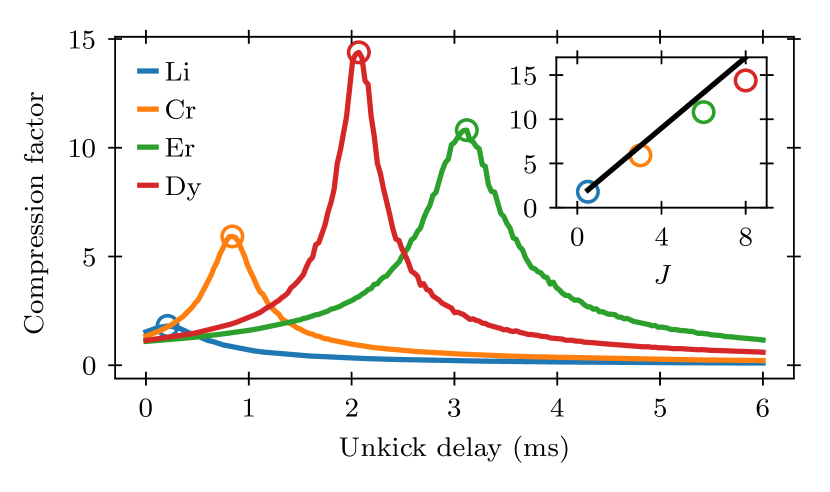
Figure 4: Optimizing the wait time between the MOP cooling kick and unkick according to the compression factor. The open circle marks the optimal delay time for each species subject to the initial conditions and magnetic forces described in the text. The inset shows the peak compression factor vs the species’ angular momentum $J$, compared to the geometric limit $2J+1$ (black line).

We now generalize the method to a system with an arbitrary total angular momentum $J$. There are $2J+1$ states in this case, and we assume that the atoms are trapped in a hard-walled flat potential. Just as in the case of Li above, we turn off the trap to start the cooling sequence. Using optical pumping and stimulated transitions in step (1), the cloud is divided into $2J+1$ equally-sized components, where the leftmost section is prepared in state $\left|J,-J\right\rangle$, then $\left|J,-J+1\right\rangle$, and so on, to the rightmost section in state $\left|J,J\right\rangle$. In step (2), a magnetic field gradient kick is applied to the cloud, causing each sub-section to move at a velocity that is proportional to its distance from the center-plane. Thus, the stretched states $\left|J,\pm J\right\rangle$ will move the fastest towards the center, and lower magnetic-quantum-numbered sections will move slower. The cloud will collapse to a single section after an optimal delay time, and a reverse magnetic kick will restore the original velocity distributions. Finally, in step (3), all atoms are optically pumped to the $\left|J,J\right\rangle$ state, and the cloud can be re-trapped. Ideally, the cloud has been compressed by a factor of $2J+1$.

Figures 3 (e - h) show snapshots of the simulated phase-space for MOP cooling of Dy atoms ($J=8$) after state preparation (step 1) and during magnetic kicking (step 2). Comparing the final spatial distribution of Li [Fig. 3 (d)] to that of Dy [Fig. 3 (h)] clearly demonstrates how MOP cooling may leverage high-angular-momentum atoms for efficient phase-space compression.

The delay time between kicks is optimized in our numeric simulations and the results are shown for a variety of atoms in Fig. 4. As a figure of merit, we compute the compression factor as the ratio of standard deviations between the initial and final $z$-coordinate distributions of the cloud. The inset of Fig. 4 shows the peak compression factor for each species is bound by the geometric limit $2J+1$. In the following section we consider some limitations of MOP cooling and how they may be overcome in an experiment.

3 Discussion

In MOP cooling, a maximum compression factor of $2J+1$ per cycle may be approached. However, in practice, the efficiency will be lower due to thermal expansion, deviations from a flat density distribution, imperfect kicking fields, and photon-recoil heating during the optical pumping stage.

To better understand the influence of thermal expansion and the initial density profile, we have developed a one-dimensional analytic model of MOP cooling that is reported in the Appendix. A few key conclusions derived from our model are now summarized. While the MOP cooling sequence progresses, the atomic ensemble’s initial standard deviation $\sigma_{0}$ grows according to $\sigma(t)=\sqrt{\sigma_{0}^{2}+t^{2}v_{\rm th}^{2}}$ where $v_{\rm th}=\sqrt{k_{\rm B}T/M}$ is the thermal velocity. Thus, after a MOP cooling sequence, the ensemble has collapsed to a single section, but the sections have grown from their initial size. The total time for one sequence is $t_{0}+\tau$ and for simplicity let us assume $t_{0}\gg 2\tau$, i.e. the delay time between kicks is much longer than the kicks’ combined pulse length. Additionally, a flat distribution of width $2s$ has a standard deviation $\sigma=2s/\sqrt{12}$, so the thermally-limited compression factor is approximately $(2J+1)/\sqrt{1+12v_{\rm th}^{2}/\Delta v^{2}}$ where $\Delta v=2g_{J}\mu_{\rm B}G\tau/M\pi$ is the relative kick velocity of adjacent sections and $G$ is the peak field gradient. Thus, the geometric limit $2J+1$ is only achieved for $\Delta v\gg\sqrt{12}v_{\rm th}$.

The flat-density initial condition is quite different from that usually encountered with laser cooled atoms in a magneto-optical trap, but turns out to be important for the gains in efficiency that are predicted (details in the Appendix). For example, we predict a compression factor of 1.8 for Li initialized with with a flat density or 1.5 for a Gaussian distribution. For Dy initialized with a flat density, a peak compression factor of 14.4 is observed, while for an initially-Gaussian distribution the factor reduces to 8.6. To obtain a flat “boxlike” distribution in an experiment, the atoms can first be confined in a magnetic quadrupole trap. An optical box can be created around the atoms using a time-averaged optical dipole potential from beams that are moving rapidly in two dimensions. Such potentials were created in the past to study optical billiards [32, 33] and BECs in painted potentials [34]. After trapping, the box can be adiabatically expanded in three dimensions to a desired size, which will result in a nearly flat density profile of atoms. The optical setup for state preparation of each segment would enable multiple cycles of cooling in each dimension. Adiabatic expansion would lower the kinetic energy and MOP cooling would compress the cloud spatially. The process can be dynamically controlled with motorized zoom lenses [35].

Ideally, a complete cycle of MOP cooling leaves the velocity distribution of the atomic sample unchanged. This means that the momentum imparted on the atoms in the kick phase must be nulled in the reverse-kick phase. Inhomogeneities in the kicking field will result in a nonzero mean velocity for the cloud. Such inhomogeneities are noticeable in Fig. 2 (b) that shows the peak magnetic field gradient in the $x=0$ plane. For instance, atoms near $z=0.25$ will be kicked downward with slightly less force than their upward motion-arresting kick that is applied once they are near $z=0$. Our simulations suggest this effect is negligible for the chosen field and cloud parameters, but it becomes relevant for larger clouds or less uniform field gradients. Moreover, there exist advanced wiring-design-optimization techniques to generate uniform bias or gradient fields with minimal inductance [36, 28]. Though originally developed for magnetic resonance imaging, MOP cooling could benefit from such analyses to improve switching times of the pulsed magnetic fields and increase the uniformity of the required biased gradients, thereby enabling MOP cooling of larger ensembles. A possibly more significant mean velocity is incurred due to free fall in the Earth’s gravitational field. For example, in the $\sim 3.5$ ms of delay time required for MOP cooling of Cr, the cloud accelerates to nearly 3.5 cm/s and displaces 0.67 mm. Such velocities and displacements are within typical capture ranges of atomic traps, though some loss upon re-trapping should be expected. To mitigate the free fall effects, one could use the MOP cooling setup to apply an additional uniform kicks against gravity.

In general, optically pumping the cloud to the same magnetic state is a lossy step due to, for instance, atoms decaying to unobserved trap states. Fortunately, there exist efficient techniques for optical pumping as discussed in [37], where it is shown that it is possible to perform optical pumping with only one spontaneous photon emitted per atom. The same physics lets us understand MOP cooling’s high phase-space compression efficiency in terms of the photon entropy carried away from the ensemble by spontaneous emission [38].

The entropy associated with the motional degrees of freedom is given by $S_{\rm mo.}=k_{\rm B}\ln(V/V_{\rm Q})$, where $V$ is the phase-space volume and $V_{\rm Q}$ is a reference volume. The ensemble’s volume is reduced by a factor of (at most) $2J+1$ at each cooling step, so the maximum entropy reduction per step is $\Delta S_{\rm mo.}=k_{\rm B}\ln{(2J+1)}$. The magnetic kicks are reversible evolution, so they do not produce a net change in entropy. Therefore the entropy change must occur during the optical pumping step. Optical pumping of an unpolarized ensemble to produce a pure state reduces the polarization entropy by $\Delta S_{\text{pol.}}=k_{\rm B}\ln{(2J+1)}$. Thus for each step, (1) optical pumping takes unpolarized state to pure state, reducing polarization entropy by $k_{\rm B}\ln{(2J+1)}$; (2) magnetic kicks take the pure state to an unpolarized one by overlapping the sub-ensembles, increasing polarization entropy by $k_{\rm B}\ln{(2J+1)}$ and reducing motional entropy by the same amount. The cooling must ultimately be limited by recoil heating. If single-photon optical pumping efficiency is achieved and spatial compression converted to temperature reduction through adiabatic expansion, the temperature limit will correspond to the recoil temperature $T_{\rm rec}$. For less efficient optical pumping the temperature limit will be higher.

The conceptual significance of MOP cooling is two-fold. First, in species that have already reached quantum degeneracy with the aid of laser cooling, MOP cooling can reduce losses induced by the typical final step of evaporation. Alternative all-optical approaches have produced degenerate ${}^{87}{\rm Rb}$ samples while avoiding evaporation: Raman cooling in combination with either optical compression cycles [39] or far-off-resonant optical pumping [40] have reached degeneracy within 300 ms or 1.4 s, respectively. The present simulations predict that a single cycle of MOP cooling for Dy will compress the extent of the ensemble along one dimension by a factor of 14.4 within just 3 ms. This compression increases the number density, and therefore also the phase-space density, by the same factor. Hence, if initially laser cooled to a phase-space density of $\sim 10^{-6}$, MOP cooling may bring Dy to degeneracy within six cycles or about 20 ms. Second, in species lacking a sufficiently-closed two-level cycling transition, MOP cooling provides an alternative technique that only requires optical pumping, coherent population transfer, and pulsed magnetic fields. Here, we have shown that the efficiency of MOP cooling can be increased by leveraging larger internal state spaces. Therefore, a particularly enticing possibility for future work is the application of MOP cooling to ultracold molecules [41, 42]. A rich internal-state structure makes laser cooling prohibitively challenging for most, though not all [43], molecular species. On the other hand, molecules may be cooled quite generally to the single-kelvin regime via buffer-gas collisions or supersonic expansion [16], and perhaps MOP cooling could push molecular ensembles to yet-higher phase-space densities.

4 Conclusion

In this paper, we proposed a highly efficient method for phase-space compression of high-angular-momentum atoms. This work extends an earlier MOP-cooling proposal from Li to general high-angular-momentum atoms. We numerically tested our new MOP-cooling protocol on four atomic species of increasing angular momenta that have each already been cooled using traditional techniques. We find, for example, an impressive compression factor of 14.4 is conceivably attainable in less than 3 ms for the case of Dy.

Appendix: One-dimensional model

In this appendix, we develop a one-dimensional model for MOP cooling. We consider the compression limits imposed by 1) geometry of the initial spatial distribution of atoms and 2) thermal free expansion during the required time-of-flight to complete a MOP cooling cycle. To this end, we begin with the more complicated case of an initially-Gaussian spatial distribution. Ignoring free expansion, we determine an optimal partitioning scheme that splits the initial distribution into $2J+1$ sections. Then, we consider how the shape of each Gaussian partition changes over the time of flight required to merge the sections. Finally, we repeat the analysis for an initially flat distribution.

A.1 General setup

Consider a one-dimensional, classical, non-interacting gas composed of a constant number of atoms with mass $M$ trapped in a potential $V(x)$ and in thermal equilibrium at temperature $T$. The energy of an atom is $Mv^{2}/2+V(x)$ when it is at position $x$ with velocity $v$. The probability for an atom to be found in the phasespace area $(x+dx)\times(v+dv)$ is $\rho(x,v)dxdv$ where the probability density is given by the Boltzmann factor

$$\rho(x,v)=\rho_{0}e^{-[Mv^{2}/2+V(x)]/k_{\rm B}T},$$ (1)

where the constant $\rho_{0}$ normalizes the density such that it integrates to unity. Therefore, the real-space probability density is given by the marginal

$$\mathcal{P}(x)=\int_{-\infty}^{\infty}{\rm d}v\rho(x,v)=\rho_{0}\sqrt{2\pi v_{\rm th}^{2}}e^{-V(x)/k_{\rm B}T},$$ (2)

where we have defined the thermal velocity $v_{\rm th}=\sqrt{k_{\rm B}T/M}$.

In MOP cooling we imagine slicing the initial density distribution $\mathcal{P}(x)$ into $2J+1$ sections, where the left-most section is labeled by $m_{J}=-J$, followed by $-J+1$, and so on to the right most section labeled $m_{J}=J$. Then, each section is kicked to a velocity $v_{0}\propto-m_{J}$ such that the distribution is compressed. Our goal is to develop a model allowing us to optimize the MOP cooling protocol for maximum compression. As a figure of merit, we compute the compression factor as the initial-to-final ratio $\mathcal{R}$ of the spatial distribution’s standard deviation. We restrict our attention to cases in which $\mathcal{P}$ remains symmetric around $x=0$ so that the distribution’s standard deviation is the square-root of its second moment. Therefore, the compression factor is $\mathcal{R}\equiv\sqrt{\langle x^{2}\rangle_{\mathcal{P}_{\rm initial}}/\langle x^{2}\rangle_{\mathcal{P}_{\rm final}}}$ where

$$\langle x^{2}\rangle_{\mathcal{P}}=\int_{-\infty}^{\infty}{\rm d}x\,x^{2}\mathcal{P}(x).$$ (3)

Note that maximizing $\mathcal{R}$ is equivalent to minimizing $\mathcal{R}^{-2}$, i.e. the ratio of the distribution’s final-to-initial variance.

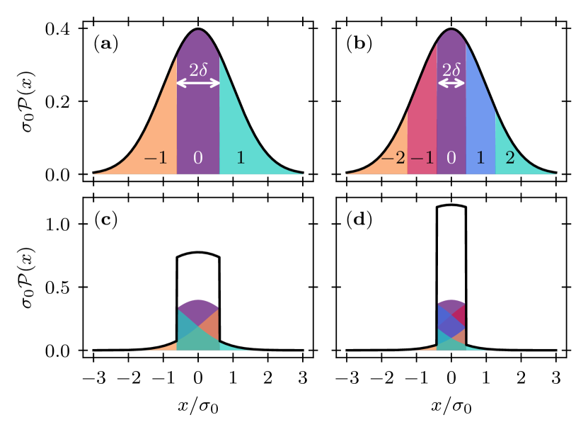
Figure 5: The initially Gaussian (a-b) and final (c-d) distributions for MOP cooling of with $J=1$ [(a) and (c)] and $J=2$ [(b) and (d)]. Colors correspond to $m_{J}$ sections, as labeled in panels (a) and (b), and the black lines mark the total distribution. Here, $\delta$ was chosen according to Equation (11).

A.2 Compression limits for a Gaussian distribution

When trapped in a harmonic potential $V(x)=M\omega_{0}^{2}x^{2}/2$, the real-space probability density is Gaussian

$$\mathcal{P}_{\rm G}(x)=\frac{1}{\sqrt{2\pi\sigma_{0}^{2}}}e^{-x^{2}/2\sigma_{0}^{2}},$$ (4)

where we have evaluated the phase-space normalization constant $\rho_{0}=1/2\pi v_{\rm th}\sigma_{0}$ and defined the density’s variance $\sigma_{0}^{2}=k_{\rm B}T/M\omega_{0}^{2}$. The initial standard deviation in this case is simply $\sigma_{0}=v_{\rm th}/\omega_{0}$.

Define the the intervals $(a,b)_{m_{J}}$ that specify the partitioning of the initial distribution as

$$(a,b)_{m_{J}}=\delta\sigma_{0}\cases{(-\infty,\,-(2J+1)]&$m_{J}=-J$\\ ((2m_{J}-1),\,(2m_{J}+1)]&$|m_{J}|<J$\\ ((2J-1),\,\infty)&$m_{J}=J$\\ }$$ (5)

where $2\delta>0$ represents the distance between adjacent sections in units of $\sigma_{0}$. At the end of a MOP cooling cycle, these sections have collapsed. Figure 5 depicts examples of the initial and final distributions for $J=1,2$.

A.2.1 Geometric limit

If the section collapse occurs much faster than thermal free expansion, then the observed compression is limited by the initial distribution’s shape. Typographically, we will use a hat over functions and optimized variables to distinguish this geometric limit from the more general results presented later, which account for thermal free expansion. In the present case of an initially-Gaussian distribution, the final distribution is

$$\hat{\mathcal{P}}(x)=\cases{\mathcal{P}_{\rm G}(x-2J\delta\sigma_{0})&$x<-\delta\sigma_{0}$\\ \sum\limits_{m_{J}=-J}^{J}\mathcal{P}_{\rm G}(x-2m_{J}\delta\sigma_{0})&$|x|<\delta\sigma_{0}$\\ \mathcal{P}_{\rm G}(x+2J\delta\sigma_{0})&$x>\delta\sigma_{0}$ .}$$ (6)

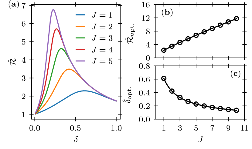
Figure 6: (a) The compression factor for various ways of splitting and merging a Gaussian distribution, as given by Equation (7). We numerically extract the peak compression factor $\hat{\mathcal{R}}_{\rm opt}$ and corresponding relative half-width $\hat{\delta}_{\rm opt.}$ and show their $J$-scaling in panels (b) and (c), respectively. The solid lines in (b) and (c) result from the simultaneous fit to Equations (10) and (11), respectively.

As for the compression factor $\hat{\mathcal{R}}$, the required integral (3) may be evaluated to give

$$\hat{\mathcal{R}}^{-2}(\delta,J)=1-2\delta S_{1}(\delta,J)+4\delta^{2}\left[J^{2}-S_{2}(\delta,J)\right],$$ (7)

which is valid for both integer and half-integer $J$ and where we have defined the two parameterized summations

$$S_{1}(\delta,J)=\sqrt{\frac{2}{\pi}}\sum_{m_{J}=-J}^{J-1}\exp\left[\frac{-\delta^{2}(2m_{J}+1)^{2}}{2}\right]$$ (8)

$$S_{2}(\delta,J)=\frac{1}{2}\sum_{m_{J}=-J}^{J-1}(2m_{J}+1){\rm Erf}\left[\frac{\delta(2m_{J}+1)}{\sqrt{2}}\right].$$ (9)

In Figure 6 (a) we show $\hat{\mathcal{R}}$ as a function of $\delta$ for various $J$.

Equation (7) provides a way to optimize $\delta$ for a given $J$ by solving $\partial\hat{\mathcal{R}}^{-2}/\partial\delta=0$ for $\delta\equiv\hat{\delta}_{\rm opt}$. Using the identity $S_{1}^{\prime}(\delta,J)/S_{2}^{\prime}(\delta,J)=-2\delta$, where the prime denotes a derivative with respect to $\delta$, we deduce $4\hat{\delta}_{\rm opt.}[J^{2}-S_{2}(\hat{\delta}_{\rm opt.},J)]-S_{1}(\hat{\delta}_{\rm opt.},J)=0$. Thus, the corresponding optimal compression factor $\hat{\mathcal{R}}_{\rm opt.}(J)=\hat{\mathcal{R}}(\delta_{\rm opt.},J)$ is given by $\hat{\mathcal{R}}^{-2}_{\rm opt.}=1-\hat{\delta}_{\rm opt.}S_{1}(\hat{\delta}_{\rm opt.},J)$. The transcendental form of the above optimization equations precludes a closed form solution. Fortunately, numeric root finding allows us to quickly and accurately obtain $\hat{\delta}_{\rm opt.}$. Empirically, we find that the numerically-optimized $\hat{\delta}_{\rm opt.}(J)$ and the corresponding $\hat{\mathcal{R}}_{\rm opt.}(J)$ are well fit, simultaneously, to the models,

$$\hat{\mathcal{R}}_{\rm opt.}(J)\approx A_{1}(2J+1)^{B}$$ (10)

$$\hat{\delta}_{\rm opt.}(J)\approx A_{2}(2J+A_{3})^{-B}\,,$$ (11)

as shown in Figure 6 (b-c). Our fit yields $A_{1}=0.89$, $A_{2}=1.82$, $A_{3}=1.61$, and $B=0.85$. The fitted functions and numeric optimizations agree with an average relative error of 0.33% for $\hat{\mathcal{R}}_{\rm opt.}$ and 0.08% for $\hat{\delta}_{\rm opt.}$ for integer $1\leq J\leq 10$.

A.2.2 Thermal limit

Due to finite magnetic kick strengths, MOP cooling requires a finite time-of-flight to reach peak compression. Due to the ensemble’s finite temperature, the spatial and velocity distributions correlate via free expansion, meaning each section becomes more Gaussian-like over the required time-of-flight. Towards a model of MOP cooling including these effects, let us compute the time-dependence of an initially-Gaussian spatial distribution subject to thermal free expansion and translation at a constant kicking velocity $v_{0}$. We are particularly interested in the time dependence of a subsection of such a distribution that initially occupies the interval $(a,b)$, denoted $\mathcal{P}_{\rm sec.}\left[x,t;v_{0},(a,b)\right]$. Microscopically, the atom trajectories obey $\dot{v}=0$ and $\dot{x}=v+v_{0}$, so, by Liouville’s theorem, we may write the time-dependent phase-space density as $\rho(x-(v+v_{0})t,v)$. The real-space marginal is

$$\mathcal{P}_{\rm sec.}\left[x,t;v_{0},(a,b)\right]=\frac{1}{2\pi\sigma_{0}v_{\rm th}}\int_{\frac{x-b}{t}-v_{0}}^{\frac{x-a}{t}-v_{0}}{\rm d}v\,$$ (12)

$$\qquad\times\exp\left(-\frac{v^{2}}{2v_{\rm th}^{2}}-\frac{[x-t(v+v_{0})]^{2}}{2\sigma_{0}^{2}}\right)$$

$$=\frac{1}{2\sqrt{2\pi\sigma_{0}^{2}f^{2}_{t}}}\exp\left(\frac{-[x-tv_{0}]^{2}}{2\sigma^{2}_{0}f^{2}_{t}}\right)$$

$$\qquad\times\left[{\rm Erf}\left(\frac{bf_{t}^{2}+tv_{0}-x}{\sqrt{2}f_{t}v_{\rm th}t}\right)-{\rm Erf}\left(\frac{af_{t}^{2}+tv_{0}-x}{\sqrt{2}f_{t}v_{\rm th}t}\right)\right]$$

where we have defined $f^{2}_{t}=1+t^{2}v_{\rm th}^{2}/\sigma_{0}^{2}$ and ${\rm Erf}$ is the error function. When $(a,b)=(-\infty,\,\infty)$, then the factor in square brackets becomes $2$, and the result is familiar from time-of-flight analysis of harmonically trapped ensembles. To model MOP cooling, we set the kicking velocity to $v_{0}=-m_{J}\gamma v_{\rm th}$, where $\gamma>0$ measures the kicking strength in units of the thermal velocity, and then sum the distribution sections over the intervals given in Equation (5):

$$\mathcal{P}(x,t)=\sum_{m_{J}=-J}^{J}\mathcal{P}_{\rm sec.}\left[x,t;-m_{J}\gamma v_{\rm th},(a,b)_{m_{J}}\right].$$ (13)

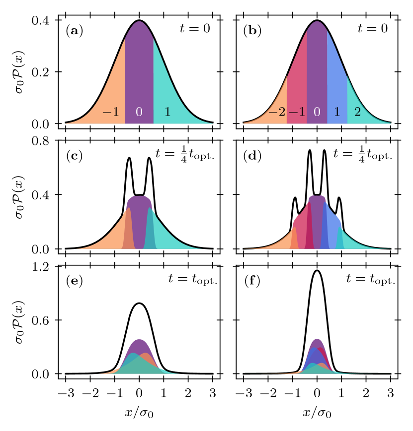
Figure 7: Time-dependent MOP cooling model for a kicking strength of $\gamma=5$ and including effects of free expansion. The initial distributions are shown for (a) $J=1$ and (b) $J=2$. Similarly, panels (c) and (d) show this distributions after a time $t_{\rm opt.}/4$ for $J=1$ and $J=2$, respectively. After a time $t_{\rm opt.}$ the distributions have minimal variance and are shown shown for (e) $J=1$ and (f) $J=2$.

Figure 7 shows the time-dependent, real-space probability density for $J=1,2$ and $\gamma=5$ at times $t=0$, $t=t_{\rm opt.}/4$, and $t=t_{\rm opt.}$ where $t_{\rm opt.}\approx 2\delta\sigma_{0}/\gamma v_{\rm th}$ is the optimal delay time after which the sections have collapsed.

From the probability density (13) we may evaluate the compression factor $\mathcal{R}$. It is convenient to introduce the non-dimensional time $\tau$ such that $t=\tau\sigma_{0}/v_{\rm th}$. Then, the final result reads

$$\mathcal{R}^{-2}(\tau,\delta,\gamma,J)=1 -\tau\gamma S_{1}(\delta,J)$$

$$+\tau^{2}\left[1+\gamma^{2}J^{2}-\gamma^{2}S_{2}(\delta,J)\right].$$

The geometric limit (7) is recovered from (A.2.2) for $\gamma\to\infty$ and $\tau\to 0$ such that $\tau\gamma\to 2\delta$.

From (A.2.2), the optimal delay time $t_{\rm opt.}=\tau_{\rm opt.}v_{\rm th}/\sigma_{0}$ may be expressed in closed form upon solving $\partial\mathcal{R}^{-2}/\partial\tau=0$ for $\tau\equiv\tau_{\rm opt.}$, yielding

$$\tau_{\rm opt.}(\delta,\gamma,J)=\frac{\gamma}{2}\frac{S_{1}(\delta,J)}{1+\gamma^{2}J^{2}-\gamma^{2}S_{2}(\delta,J)}.$$ (15)

On the other hand, optimizing $\mathcal{R}$ with respect to the relative half-width $\delta_{\rm opt.}$ for given angular momentum $J$ and kick strength $\gamma$ requires numeric minimization of equation (A.2.2). Similarly to the geometric-limit case, analytic optimization implies $4\delta_{\rm opt.}[1+\gamma^{2}J^{2}-\gamma^{2}S_{2}(\delta_{\rm opt.},J)]-\gamma^{2}S_{1}(\delta_{\rm opt.},J)=0$ and ${\mathcal{R}}^{-2}_{\rm opt.}(\gamma,J)=1-\delta_{\rm opt.}S_{1}(\delta_{\rm opt.},J)$ where $\mathcal{R}_{\rm opt.}(\gamma,J)=\mathcal{R}(\tau_{\rm opt},\delta_{\rm opt.},\gamma,J)$.

A.3 Compression limits for a flat distribution

When trapped in a box-like potential of width $2s_{0}$, $V(|x|>s_{0})=\infty$ and $V(|x|\leq s_{0})=0$, the ensemble’s spatial distribution $\mathcal{P}_{\rm F}(|x|<s_{0})=1/2s_{0}$ is flat and has a standard deviation $\sigma_{0}=s_{0}/\sqrt{3}$. For a flat distribution, deciding how to partition the $(2J+1)$ sections for MOP cooling is simpler than in the Gaussian case. The flat distribution only has support over the interval $(-s_{0},\,s_{0})$, so it is intuitive to split the initial distribution into a number $2J+1$ of equally sized sections such that each section contains an equal number of atoms. That is, the intervals of each section are finite and given by

$$(a,b)_{m_{J}}=\left(s_{0}\frac{2m_{J}-1}{2J+1},\,s_{0}\frac{2m_{J}+1}{2J+1}\right).$$ (16)

In the geometric limit, all sections remain flat and merge to a single section of width $2s_{0}/(2J+1)$ and hence the geometrically-limited compression factor is $\hat{\mathcal{R}}_{\rm opt.}(J)=2J+1$.

Including the effects of thermal and mean velocity, we find the time-dependent spatial distribution of a section initially occupying the interval $(a,b)$ is

$$\mathcal{P}_{\rm sec.}[x,t;v_{0},(a,b)]=\frac{1}{4s_{0}}\bigg{[} {\rm Erf}\left(\frac{b-x+tv_{0}}{\sqrt{2}tv_{\rm th}}\right)$$

$$-{\rm Erf}\left(\frac{a-x+tv_{0}}{\sqrt{2}tv_{\rm th}}\right)\bigg{]}.$$

As in Equation (13), the kicking velocities for each section are $v_{0}=-m_{J}\gamma v_{\rm th}$ and the total distribution is the sum of each section’s distribution. The initial variance is given by $\sigma^{2}_{0}=s_{0}^{2}/3$. Introducing the non-dimensional time $\tau=tv_{\rm th}/s_{0}$ allows us to express the compression factor as

$$\mathcal{R}^{-2}(\tau,\gamma,J)=1 -\tau\gamma\frac{4J(J+1)}{(2J+1)}$$

$$+\tau^{2}\left[3+\gamma^{2}J(J+1)\right].$$

Equation (A.3) connects to the simulations discussed in the main text. In Figure 8 we compare Equation (A.3) to the simulation results presented in Figure 4. We have set $T=25T_{\rm rec}$ and $\gamma=\Delta v/v_{\rm th}$ where $\Delta v=2g_{J}\mu_{\rm B}G\tau/M\pi$ is the relative kick velocity of adjacent sections and $G$ is the peak field gradient. With no remaining free parameters our one-dimensional model and simulations, which include realistic kicking profiles, are in excellent agreement.

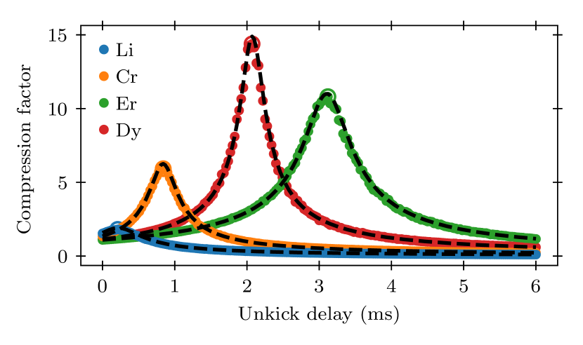
Figure 8: The data points are reproduced from Figure 4 of the main text and the dashed lines correspond to Equation (A.3), to the minus-one-half power, with $\gamma$ and $v_{\rm th}$ set in accordance with the simulations, i.e., no free parameters.

For large enough $\gamma$, we expect the time at which $\mathcal{R}$ is maximized is when all sections have merged at $t_{\rm opt.}\approx 2s_{0}/\gamma v_{\rm th}(2J+1)$. At this time, the compression factor according to Equation (A.3) evaluates to

$$\mathcal{R}_{\rm opt.}(\gamma,J)\approx\frac{(2J+1)}{\sqrt{1+12/\gamma^{2}}}.$$ (19)

Equation (19) is identical to that given in the discussion section of the main text. More precisely, solving $\partial\mathcal{R}^{-2}/\partial\tau=0$ for $\tau\equiv\tau_{\rm opt.}$ gives

$$\tau_{\rm opt.}(\gamma,J)=\frac{2\gamma J(J+1)}{(2J+1)\left[3+\gamma^{2}J(J+1)\right]}$$ (20)

$$=\frac{2}{\gamma(2J+1)}+\mathcal{O}(\gamma^{-2})$$

$$\mathcal{R}_{\rm opt.}(\gamma,J)=(2J+1)\left[\frac{3+\gamma^{2}J(J+1)}{3+J(J+1)(\gamma^{2}+12)}\right]^{1/2}.$$ (21)

The second equality in (20) comes from a first order expansion in $\gamma^{-1}$ and recovers our $\gamma\to\infty$ expectation. Approximation (19) is accurate to better than 10% (1%) of Equation (21) when $\gamma\geq 2$ and $J=1$ ($J=5$), and accuracy improves monotonically with increasing $\gamma$ and $J$.

The one-dimensional models defined in this appendix are useful to understand the scaling properties of MOP cooling for both Gaussian and flat density profiles. We have outlined techniques for optimization that provide engineering specifications and enable sensitivity analyses for the design of real experimental systems. In the main text, we focused on atomic simulations rather than the models defined here because they not only include thermal free expansion effects, but also three-dimensional, time-dependent kicking forces. In the future, it may be possible to extend our models to include effects like kicking inhomogeneities and finite kicking duration as well as quantum-statistical effects and state preparation details ignored by the main-text simulations.

References

References

- [1] Harold J Metcalf and Peter Van der Straten. Laser cooling and trapping. Springer Science & Business Media, 1999.
- [2] Florian Schreck and Klaasjan van Druten. Laser cooling for quantum gases. Nature Physics, 17(12):1296–1304, 2021.
- [3] Paul D Lett, Richard N Watts, Christoph I Westbrook, William D Phillips, Phillip L Gould, and Harold J Metcalf. Observation of atoms laser cooled below the doppler limit. Physical Review Letters, 61(2):169, 1988.
- [4] Jean Dalibard and Claude Cohen-Tannoudji. Laser cooling below the doppler limit by polarization gradients: simple theoretical models. Journal of the Optical Society of America B, 6(11):2023–2045, 1989.
- [5] P Jeffery Ungar, David S Weiss, Erling Riis, and Steven Chu. Optical molasses and multilevel atoms: theory. Journal of the Optical Society of America B, 6(11):2058–2071, 1989.
- [6] David S Weiss, Erling Riis, Yaakov Shevy, P Jeffrey Ungar, and Steven Chu. Optical molasses and multilevel atoms: experiment. Journal of the Optical Society of America B, 6(11):2072–2083, 1989.
- [7] AM Steane and CJ Foot. Laser cooling below the doppler limit in a magneto-optical trap. Europhysics Letters, 14(3):231, 1991.
- [8] Vladan Vuletić, Cheng Chin, Andrew J Kerman, and Steven Chu. Degenerate raman sideband cooling of trapped cesium atoms at very high atomic densities. Physical Review Letters, 81(26):5768, 1998.
- [9] Andrew J Kerman, Vladan Vuletić, Cheng Chin, and Steven Chu. Beyond optical molasses: 3d raman sideband cooling of atomic cesium to high phase-space density. Physical Review Letters, 84(3):439, 2000.
- [10] Harald F Hess. Evaporative cooling of magnetically trapped and compressed spin-polarized hydrogen. Physical Review B, 34(5):3476, 1986.
- [11] Naoto Masuhara, John M Doyle, Jon C Sandberg, Daniel Kleppner, Thomas J Greytak, Harald F Hess, and Greg P Kochanski. Evaporative cooling of spin-polarized atomic hydrogen. Physical Review Letters, 61(8):935, 1988.
- [12] M-O Mewes, MR Andrews, DM Kurn, DS Durfee, CG Townsend, and W Ketterle. Output coupler for bose-einstein condensed atoms. Physical Review Letters, 78(4):582, 1997.
- [13] MR Andrews, CG Townsend, H-J Miesner, DS Durfee, DM Kurn, and W Ketterle. Observation of interference between two bose condensates. Science, 275(5300):637–641, 1997.
- [14] Immanuel Bloch, Theodor W Hänsch, and Tilman Esslinger. Atom laser with a cw output coupler. Physical Review Letters, 82(15):3008, 1999.
- [15] Mark G Raizen. Comprehensive control of atomic motion. Science, 324(5933):1403–1406, 2009.
- [16] Dima Egorov, Thierry Lahaye, Wieland Schöllkopf, Bretislav Friedrich, and John M Doyle. Buffer-gas cooling of atomic and molecular beams. Physical Review A, 66(4):043401, 2002.
- [17] MG Raizen, AM Dudarev, Qian Niu, and NJ Fisch. Compression of atomic phase space using an asymmetric one-way barrier. Physical Review Letters, 94(5):053003, 2005.
- [18] Gabriel N Price, S Travis Bannerman, Kirsten Viering, Edvardas Narevicius, and Mark G Raizen. Single-photon atomic cooling. Physical Review Letters, 100(9):093004, 2008.
- [19] Jeremy J. Thorn, Elizabeth A. Schoene, Tao Li, and Daniel A. Steck. Experimental realization of an optical one-way barrier for neutral atoms. Physical Review Letters, 100:240407, Jun 2008.
- [20] Mark G Raizen, Dmitry Budker, Simon M Rochester, Julia Narevicius, and Edvardas Narevicius. Magneto-optical cooling of atoms. Optics Letters, 39(15):4502–4505, 2014.
- [21] Lauriane Chomaz, Igor Ferrier-Barbut, Francesca Ferlaino, Bruno Laburthe-Tolra, Benjamin L Lev, and Tilman Pfau. Dipolar physics: A review of experiments with magnetic quantum gases. Reports on Progress in Physics, 2022.
- [22] Alfred Kastler. Quelques suggestions concernant la production optique et la détection optique d’une inégalité de population des niveaux de quantifigation spatiale des atomes. application à l’expérience de stern et gerlach et à la résonance magnétique. Journal de Physique et Le Radium, 11(6):255–265, 1950.
- [23] A. Kramida, Yu. Ralchenko, J. Reader, and and NIST ASD Team. NIST Atomic Spectra Database (ver. 5.10), [Online]. Available: https://physics.nist.gov/asd [2022, December 5]. National Institute of Standards and Technology, Gaithersburg, MD., 2022.
- [24] Randall G. Hulet, Jason H. V. Nguyen, and Ruwan Senaratne. Methods for preparing quantum gases of lithium. Review of Scientific Instruments, 91(1):011101, 2020.
- [25] C. C. Bradley, J. J. McClelland, W. R. Anderson, and R. J. Celotta. Magneto-optical trapping of chromium atoms. Physical Review A, 61:053407, Apr 2000.
- [26] A. Frisch, K. Aikawa, M. Mark, A. Rietzler, J. Schindler, E. Zupanič, R. Grimm, and F. Ferlaino. Narrow-line magneto-optical trap for erbium. Physical Review A, 85:051401, May 2012.
- [27] William Lunden, Li Du, Michael Cantara, Pierre Barral, Alan O. Jamison, and Wolfgang Ketterle. Enhancing the capture velocity of a Dy magneto-optical trap with two-stage slowing. Physical Review A, 101:063403, Jun 2020.
- [28] Robert Turner. Minimum inductance coils. Journal of Physics E: Scientific Instruments, 21(10):948, 1988.
- [29] K Bergmann, H Theuer, and BW Shore. Coherent population transfer among quantum states of atoms and molecules. Reviews of Modern Physics, 70(3):1003, 1998.
- [30] Klaas Bergmann, Hanns-Christoph Nägerl, Cristian Panda, Gerald Gabrielse, Eduard Miloglyadov, Martin Quack, Georg Seyfang, Gunther Wichmann, Silke Ospelkaus, Axel Kuhn, Stefano Longhi, Alexander Szameit, Philipp Pirro, Burkard Hillebrands, Xue-Feng Zhu, Jie Zhu, Michael Drewsen, Winfried K Hensinger, Sebastian Weidt, Thomas Halfmann, Hai-Lin Wang, Gheorghe Sorin Paraoanu, Nikolay V Vitanov, Jordi Mompart, Thomas Busch, Timothy J Barnum, David D Grimes, Robert W Field, Mark G Raizen, Edvardas Narevicius, Marcis Auzinsh, Dmitry Budker, Adriana Pálffy, and Christoph H Keitel. Roadmap on STIRAP applications. Journal of Physics B: Atomic, Molecular and Optical Physics, 52(20):202001, sep 2019.
- [31] K. S. Melin, P. I. Nagornykh, Y. Lu, L. E. Hillberry, Y. Xu, and M. G. Raizen. Observation of a quasi-one-dimensional variation of the stern-gerlach effect. Physical Review A, 99:063417, Jun 2019.
- [32] V. Milner, J. L. Hanssen, W. C. Campbell, and M. G. Raizen. Optical billiards for atoms. Physical Review Letters, 86:1514–1517, Feb 2001.
- [33] Nir Friedman, Ariel Kaplan, Dina Carasso, and Nir Davidson. Observation of chaotic and regular dynamics in atom-optics billiards. Physical Review Letters, 86:1518–1521, Feb 2001.
- [34] Kevin Henderson, Changhyun Ryu, Calum MacCormick, and M. G. Boshier. Experimental demonstration of painting arbitrary and dynamic potentials for bose–einstein condensates. New Journal of Physics, 11(4):043030, 2009.
- [35] Toshiya Kinoshita, Trevor Wenger, and David S. Weiss. All-optical bose-einstein condensation using a compressible crossed dipole trap. Physical Review A, 71:011602, Jan 2005.
- [36] Jing Wang, Binquan Zhou, Xu Liu, Wenfeng Wu, Linlin Chen, Bangcheng Han, and Jiancheng Fang. An improved target-field method for the design of uniform magnetic field coils in miniature atomic sensors. IEEE Access, 7:74800–74810, 2019.
- [37] Simon M. Rochester, Konrad Szymański, Mark Raizen, Szymon Pustelny, Marcis Auzinsh, and Dmitry Budker. Efficient polarization of high-angular-momentum systems. Physical Review A, 94:043416, Oct 2016.
- [38] John P. Bartolotta, Simon B. Jäger, Jarrod T. Reilly, Matthew A. Norcia, James K. Thompson, Graeme Smith, and Murray J. Holland. Entropy transfer from a quantum particle to a classical coherent light field. Physical Review Research, 4:013218, Mar 2022.
- [39] Jiazhong Hu, Alban Urvoy, Zachary Vendeiro, Valentin Crépel, Wenlan Chen, and Vladan Vuletić. Creation of a bose-condensed gas of 87rb by laser cooling. Science, 358(6366):1078–1080, 2017.
- [40] Alban Urvoy, Zachary Vendeiro, Joshua Ramette, Albert Adiyatullin, and Vladan Vuletić. Direct laser cooling to bose-einstein condensation in a dipole trap. Physical Review Letters, 122(20):203202, 2019.
- [41] MD Di Rosa. Laser-cooling molecules: Concept, candidates, and supporting hyperfine-resolved measurements of rotational lines in the ax (0, 0) band of cah. The European Physical Journal D: Atomic, Molecular, Optical and Plasma Physics, 31:395–402, 2004.
- [42] Lincoln D Carr, David DeMille, Roman V Krems, and Jun Ye. Cold and ultracold molecules: science, technology and applications. New Journal of Physics, 11(5):055049, 2009.
- [43] Justin J. Burau, Parul Aggarwal, Kameron Mehling, and Jun Ye. Blue-detuned magneto-optical trap of molecules. Physical Review Letters, 130:193401, May 2023.