Doubly Optimal No-Regret Learning in Monotone Games

Abstract

We consider online learning in multi-player smooth monotone games. Existing algorithms have limitations such as (1) being only applicable to strongly monotone games; (2) lacking the no-regret guarantee; (3) having only asymptotic or slow $\mathcal{O}(\frac{1}{\sqrt{T}})$ last-iterate convergence rate to a Nash equilibrium. While the $\mathcal{O}(\frac{1}{\sqrt{T}})$ rate is tight for a large class of algorithms including the well-studied extragradient algorithm and optimistic gradient algorithm, it is not optimal for all gradient-based algorithms. We propose the accelerated optimistic gradient (AOG) algorithm, the first doubly optimal no-regret learning algorithm for smooth monotone games. Namely, our algorithm achieves both (i) the optimal $\mathcal{O}(\sqrt{T})$ regret in the adversarial setting under smooth and convex loss functions and (ii) the optimal $\mathcal{O}(\frac{1}{T})$ last-iterate convergence rate to a Nash equilibrium in multi-player smooth monotone games. As a byproduct of the accelerated last-iterate convergence rate, we further show that each player suffers only an $\mathcal{O}(\log T)$ individual worst-case dynamic regret, providing an exponential improvement over the previous state-of-the-art $\mathcal{O}(\sqrt{T})$ bound.

1 Introduction

We consider multi-agent online learning in games (Cesa-Bianchi & Lugosi, 2006), where the agents engaged in repeated play of the same game. In this model, the game (i.e., the agents’ payoff functions) is unknown to the agents, and they must learn to play the game through repeated interaction with the other agents. We focus on a rich family of multi-player games – monotone games that has been the central object of a series of recent studies in online learning and optimization (Hsieh et al., 2019; Golowich et al., 2020a, a; Lin et al., 2020; Hsieh et al., 2021; Lin et al., 2022; Cai et al., 2022b). Monotone games, first introduced by Rosen (1965), encompass many commonly studied games as special cases such as two-player zero-sum games, convex-concave games, $\lambda$-cocoercive games (Lin et al., 2020), zero-sum polymatrix games (Bregman & Fokin, 1987; Daskalakis & Papadimitriou, 2009; Cai & Daskalakis, 2011; Cai et al., 2016), and zero-sum socially-concave games (Even-Dar et al., 2009). In this paper, we investigate the following fundamental question:

How fast can the players’ day-to-day behavior converge

to a Nash equilibrium in monotone games

if players act according to a no-regret learning algorithm? (*)

In this context, “day-to-day behavior” is used to describe the collective strategy adopted by the agents during each iteration of the repeated game. Our question lies at the heart of the area of learning in games, as illustrated in (Fudenberg et al., 1998; Sorin, 2002; Cesa-Bianchi & Lugosi, 2006). The aim here is to discern whether simple and intuitive learning rules or algorithms (also termed ‘dynamics’ in game theory literature) can lead to the convergence of a joint strategy towards an equilibrium when used by agents to adapt their strategies. The presence of such a learning algorithm offers a logical explanation for the emergence of equilibrium from repetitive interactions, which may not always exhibit complete rationality.

Regret is the central metric used in online learning to measure the performance of a learning algorithm. In the classical single-agent setting, online learning considers the following repeated interaction between a player and the environment: (i) at day $t$, the player chooses an action $x_{t}\in\Omega\subseteq\mathbb{R}^{d}$; (ii) the environment selects a loss function $f_{t}(\cdot)$, and the player receives the loss $f_{t}(x_{t})$ along with some feedback (such as the loss function $f_{t}(\cdot)$, the gradient $\nabla f_{t}(x_{t})$, or just the loss $f_{t}(x_{t})$) and the process repeats. The regret is defined as the difference between the cumulative loss of the player $\sum_{t=1}^{T}f_{t}(x_{t})$ and the cumulative loss of the best fixed action in hindsight $\min_{x\in\Omega}\sum_{t=1}^{T}f_{t}(x)$. A single-agent online learning algorithm is considered no-regret if, even under an adversarially chosen sequence of loss functions, its regret at the end of round $T$ is sub-linear in $T$.

Arguably, a most common scenario, where the above online learning model instantiates, is multi-agent online learning in games. Namely, every player makes an online decision on their action and receives a loss that is determined based on their own action, as well as the actions chosen by the others. Online learning in repeated games is closely related to various applications in machine learning. To illustrate, the process of training Generative Adversarial Networks (GANs) can be perceived as a zero-sum game played recurrently between two agents (Arjovsky et al., 2017). Recent breakthroughs in game-solving, such as AlphaZero (Silver et al., 2017), AI for Stratego (Perolat et al., 2022), leverage self-play, where two agents employ the same learning algorithm to continuously compete against each other, aiming to arrive at a Nash equilibrium.

Do these learning algorithms converge in the repeated game? A well-known result states that if each player uses a no-regret learning algorithm to adapt their action, the empirical frequency of their joint action converges to a coarse correlated equilibrium (CCE) (Cesa-Bianchi & Lugosi, 2006). However, this general convergence result has two caveats: (i) the guaranteed convergence is only the empirical frequency of the players’ actions rather than the actual, day-to-day play; and (ii) the concept of CCE has limitations and may violate even the most basic rationalizability axioms (Viossat & Zapechelnyuk, 2013). Driven by these dual shortcomings, a significant body of work, as evidenced by various studies (Zhou et al., 2017a, b, 2018; Daskalakis & Panageas, 2019; Mokhtari et al., 2020a; Hsieh et al., 2019; Lei et al., 2021; Golowich et al., 2020c, a; Lin et al., 2020, 2022; Cai et al., 2022b), aims to identify specific types of games as well as no-regret learning algorithms such that the convergence can be strengthened in two principal ways:(a) attaining convergence to the more compelling solution concept of Nash equilibrium, and (b) assuring convergence in the players’ day-to-day behaviors, rather than merely in their empirical frequency of actions. In other words, the goal is to pinpoint specific games and devise no-regret learning algorithms so that the players’ action profile converges to a Nash equilibrium in the last-iterate.

Monotone games emerge as the most general class of games where such strengthened convergence result is known. Unlike in the general convergence to CCE that holds for any no-regret learning algorithms, the last-iterate convergence to Nash equilibria is more subtle and demands a careful design of the learning algorithm. For example, as demonstrated by Mertikopoulos et al. (2018), the well-known family of no-regret learning algorithms – follow-the-regularized-leader fails to converge even in two-player zero-sum games (a special case of monotone games), as the action profile of the players may cycle in space perpetually. The key to correct such cycling behavior is to introduce optimism in the algorithm. Indeed, the optimistic gradient (OG) algorithm by Popov (1980), a optimistic variant of the gradient descent algorithm, has recently been shown to exhibit an $\mathcal{O}(\frac{1}{\sqrt{T}})$ last-iterate convergence rate to a Nash equilibrium in monotone games (Golowich et al., 2020a; Cai et al., 2022b; Golowich et al., 2020b). As shown by Golowich et al. (2020a), this rate is tight for OG. However, it is not clear if $\mathcal{O}(\frac{1}{\sqrt{T}})$ is the optimal rate achievable by a no-regret algorithm.

1.1 Our Contributions

We consider multi-agent online learning in monotone games with gradient feedback. More concretely, each player $i$ at day $t$ not only observes their loss $\ell^{i}(x^{i}_{t},x^{-i}_{t})$ but also receives the gradient $\nabla_{x^{i}_{t}}\ell^{i}(x^{i}_{t},x^{-i}_{t})$.

Main Contribution

We answer question (1) by presenting a new single-agent online learning algorithm – the Accelerated Optimistic Gradient (AOG) that is doubly optimal (Theorem 5). More specifically,

Optimal regret:

AOG achieves the optimal $\mathcal{O}(\sqrt{T})$-regret in the adversarial environment;

Optimal last-iterate convergence rate:

If all players use AOG to determine their actions in a monotone game, the action profile has the optimal $\mathcal{O}(\frac{1}{T})$ last-iterate convergence rate to a Nash equilibrium.

Note that $\mathcal{O}(\frac{1}{T})$ is the fastest rate possible for solving monotone games using any gradient-based methods (Ouyang & Xu, 2021; Yoon & Ryu, 2021). Since the players only receive gradient feedback in our setting, this lower bound also applies to our problem.

Step-size adaptation.

We provide an implementation of AOG (Algorithm 1) that can automatically adapt to the environment and achieves a best-of-both-world guarantee. When deploy in an adversarial setting, Algorithm 1 obtains at most $\mathcal{O}(\sqrt{T})$-regret; when deploy in a monotone game where other players also play according to Algorithm 1, the action profile converges to a Nash equilibrium at a $\mathcal{O}(\frac{1}{T})$ rate in the last-iterate. Importantly, the adaptation does not require any communication between the players and only uses the the player’s local information. We believe such guarantee is crucial as even in a game setting, other players may not follow the same algorithm and might act arbitrarily, in which case, our algorithm still provides a guarantee on the worst-case regret.

Dynamic regret.

As an interesting byproduct of our last-iterate convergence rate, we further show that each player suffers only an $\mathcal{O}(\log T)$ individual dynamic regret, when all players play according to Algorithm 1 (Theorem 3). The dynamic regret of an algorithm is defined as the difference between the algorithm’s cumulative loss and the cumulative loss of the best action every day. The dynamic regret is notoriously difficulty to minimize, and it is well-known that a linear dynamic regret is unavoidable in the adversarial setting. In the game setting, results on dynamic regret are also sparse. To the best of our knowledge, the only sub-linear dynamic regret bound we are aware of is the $\mathcal{O}(\sqrt{T})$ dynamic regret of OG for monotone games. Our accelerated algorithm obtains an exponential improvement on the dynamic regret. See Table 1 for comparison with other well-studied learning algorithms in monotone games.

Algorithm	Adversarial Setting	Monotone Games
	No-Regret?	Rate∗	D-Regret∗∗
GD	✓	✗	$\Omega(T)$
EG	✗	$\mathcal{O}(\frac{1}{\sqrt{T}})$	$\mathcal{O}(\sqrt{T})$
OG	✓	$\mathcal{O}(\frac{1}{\sqrt{T}})$	$\mathcal{O}(\sqrt{T})$
EAG	✗	$\mathcal{O}(\frac{1}{T})$	$\mathcal{O}(\log T)$
This paper	✓	$\mathcal{O}(\frac{1}{T})$	$\mathcal{O}(\log T)$

Table 1: Existing results on learning in monotone games. (*) last-iterate convergence rate with respect to the gap function. (**) individual worst-case dynamic regret in monotone games.

Technique.

The key of our new algorithm is combining optimism with Halpern iteration (Halpern, 1967), a mechanism used in optimization to design accelerated methods. In our setting, Halpern iteration can be viewed as adding a diminishing strongly convex loss to the player’s loss function. The schedule used to decrease the added loss must be crafted carefully. If the added loss diminishes too slowly, the adversarial regret would be sub-optimal; if the added loss decreases too quickly, the algorithm may converge at a slower rate. The Halpern iteration provides a schedule that strikes the right balance and allows us to obtain the doubly optimal algorithm.

2 Preliminaries

Basic Notation.

We consider Euclidean space $(\mathbbm{R}^{n},{\mathchoice{\left\|\cdot\right\|}{\|\cdot\|}{\|\cdot\|}{\|\cdot\|}})$ where ${\mathchoice{\left\|\cdot\right\|}{\|\cdot\|}{\|\cdot\|}{\|\cdot\|}}$ is $\ell_{2}$-norm. We say a set $\mathcal{X}\subseteq\mathbbm{R}^{n}$ is bounded by $D>0$ if ${\mathchoice{\left\|x-x^{\prime}\right\|}{\|x-x^{\prime}\|}{\|x-x^{\prime}\|}{\|x-x^{\prime}\|}}\leq D$ for any $x,x^{\prime}\in\mathcal{X}$. Given a closed and convex set $\mathcal{X}\subseteq\mathbbm{R}^{n}$, the Euclidean projection operator is $\Pi_{\mathcal{X}}:\mathbbm{R}^{n}\rightarrow\mathcal{X}$ such that $\Pi_{\mathcal{X}}[x]=\operatorname*{argmin}_{x^{\prime}\in\mathcal{X}}{\mathchoice{\left\|x-x^{\prime}\right\|}{\|x-x^{\prime}\|}{\|x-x^{\prime}\|}{\|x-x^{\prime}\|}}$. For closed and convex set $\mathcal{X}$, Euclidean projection is non-expansive, i.e., ${\mathchoice{\left\|\Pi_{\mathcal{X}}[x]-\Pi_{\mathcal{X}}[x^{\prime}]\right\|}{\|\Pi_{\mathcal{X}}[x]-\Pi_{\mathcal{X}}[x^{\prime}]\|}{\|\Pi_{\mathcal{X}}[x]-\Pi_{\mathcal{X}}[x^{\prime}]\|}{\|\Pi_{\mathcal{X}}[x]-\Pi_{\mathcal{X}}[x^{\prime}]\|}}\leq{\mathchoice{\left\|x-x^{\prime}\right\|}{\|x-x^{\prime}\|}{\|x-x^{\prime}\|}{\|x-x^{\prime}\|}}$. For a closed convex set $\mathcal{X}$, the normal cone of $x\in\mathcal{X}$ is defined as $N_{\mathcal{X}}(x):=\{v:{\mathchoice{\left\langle v,x^{\prime}-x\right\rangle}{\langle v,x^{\prime}-x\rangle}{\langle v,x^{\prime}-x\rangle}{\langle v,x^{\prime}-x\rangle}}\leq 0\}$. We make use of the following properties of the normal cone: (i) for any $v\in N_{\mathcal{X}}(x)$, $x=\Pi_{\mathcal{X}}[x+v]$; (ii) if $x=\Pi_{\mathcal{X}}[x^{\prime}]$, then $x^{\prime}-x\in N_{\mathcal{X}}(x)$.

2.1 Monotone Games and Nash Equilibria

A (continuous) multi-player game is denoted as $\mathcal{G}=([N],(\mathcal{X}^{i})_{i\in[N]},(\ell^{i})_{i\in[N]})$ where $[N]=\{1,2,\ldots,N\}$ denotes the set of players. Each player $i$ chooses action from a compact and convex set $\mathcal{X}^{i}\in\mathbbm{R}^{n_{i}}$ and we write $\mathcal{X}=\prod_{i=1}^{N}\mathcal{X}^{i}\in\mathbbm{R}^{n}$ where $n=n_{1}+\cdots+n_{N}$. We always use $x^{-i}$ to denote the actions of all players except player $i$ and write $\boldsymbol{x}=(x^{i},x^{-i})=(x^{1},x^{2}\ldots,x^{N})$ as players’ action profile or strategy profile. Note that we reserve the bold $\boldsymbol{x}$ to denote the players’ action profile and use the normal $x$ to denote a single player’s action. Each player $i$ wishes to minimize a loss function $\ell^{i}(x^{i},x^{-i}):\mathcal{X}\rightarrow\mathbbm{R}$ which is continuous in $\boldsymbol{x}$ and convex in $x^{i}$. In this paper, we study learning in multi-player games with gradient feedback where after playing action profile $\boldsymbol{x}$, each player $i$ receives $V^{i}(\boldsymbol{x}):=\nabla_{x^{i}}\ell^{i}(x^{i},x^{-i})$. We define the gradient operator $V:\mathcal{X}\rightarrow\mathbbm{R}^{n}$ to be $V(\cdot)=(V^{1}(\cdot)\cdots,V^{N}(\cdot))$. The widely used solution concept for a game is Nash equilibrium, an action profile where no player gains from unilateral deviation. Formally, a Nash equilibrium of a game $\mathcal{G}$ is an action profile $\boldsymbol{x}_{\star}\in\mathcal{X}$ such that for each player $i$, it holds that $\ell^{i}(\boldsymbol{x}_{\star})\leq\ell^{i}(x^{i},x_{\star}^{-i})$ for any $x^{i}\in\mathcal{X}^{i}$.

In this paper, we study smooth monotone games where the gradient operator $V$ is $L$-Lipschitz for $L>0$:

$${\mathchoice{\left\|V(\boldsymbol{x})-V(\boldsymbol{x}^{\prime})\right\|}{\|V(\boldsymbol{x})-V(\boldsymbol{x}^{\prime})\|}{\|V(\boldsymbol{x})-V(\boldsymbol{x}^{\prime})\|}{\|V(\boldsymbol{x})-V(\boldsymbol{x}^{\prime})\|}}\leq L\cdot{\mathchoice{\left\|\boldsymbol{x}-\boldsymbol{x}^{\prime}\right\|}{\|\boldsymbol{x}-\boldsymbol{x}^{\prime}\|}{\|\boldsymbol{x}-\boldsymbol{x}^{\prime}\|}{\|\boldsymbol{x}-\boldsymbol{x}^{\prime}\|}},\forall\boldsymbol{x},\boldsymbol{x}^{\prime}\in\mathcal{X},$$

and monotone (Rosen, 1965) :

$${\mathchoice{\left\langle V(\boldsymbol{x})-V(\boldsymbol{x}^{\prime}),\boldsymbol{x}-\boldsymbol{x}^{\prime}\right\rangle}{\langle V(\boldsymbol{x})-V(\boldsymbol{x}^{\prime}),\boldsymbol{x}-\boldsymbol{x}^{\prime}\rangle}{\langle V(\boldsymbol{x})-V(\boldsymbol{x}^{\prime}),\boldsymbol{x}-\boldsymbol{x}^{\prime}\rangle}{\langle V(\boldsymbol{x})-V(\boldsymbol{x}^{\prime}),\boldsymbol{x}-\boldsymbol{x}^{\prime}\rangle}}\geq 0,\forall\boldsymbol{x},\boldsymbol{x}^{\prime}\in\mathcal{X}.$$

It is not hard to see that for smooth monotone games, a Nash equilibrium always exists. If $\boldsymbol{x}_{\star}$ is a Nash equilibrium, then a simple characterization of $\boldsymbol{x}_{\star}$ is that, for any $\boldsymbol{x}\in\mathcal{X}$, it holds that ${\mathchoice{\left\langle V(\boldsymbol{x}_{\star}),\boldsymbol{x}_{\star}-\boldsymbol{x}\right\rangle}{\langle V(\boldsymbol{x}_{\star}),\boldsymbol{x}_{\star}-\boldsymbol{x}\rangle}{\langle V(\boldsymbol{x}_{\star}),\boldsymbol{x}_{\star}-\boldsymbol{x}\rangle}{\langle V(\boldsymbol{x}_{\star}),\boldsymbol{x}_{\star}-\boldsymbol{x}\rangle}}\leq 0.$

Monotone games include many well-studied games, e.g., two-player zero-sum games, convex-concave games, $\lambda$-cocoercive games (Lin et al., 2020), strongly monotone games (such as Kelly auctions), zero-sum polymatrix games (Bregman & Fokin, 1987; Daskalakis & Papadimitriou, 2009; Cai & Daskalakis, 2011; Cai et al., 2016), and zero-sum socially-concave games (Even-Dar et al., 2009).

Example 1 (Convex-Concave Min-Max Optimization).

Given a function $f(x,y):\mathcal{X}\times\mathcal{Y}\rightarrow\mathbbm{R}$ that is convex in $x$ and concave in $y$, find a saddle point $z=(x,y)$ such that $f(x,y^{\prime})\leq f(x,y)\leq f(x^{\prime},y),\forall x^{\prime}\in\mathcal{X},y^{\prime}\in\mathcal{Y}$. It is not hard to see that the set of Nash equilibria of a two-player zero-sum game $\mathcal{G}=\{[2],(\mathcal{X},\mathcal{Y}),(f,-f)\}$ corresponds to the set of saddle points of $f$. Thus convex-concave min-max optimization is a special case of monotone games.

For a monotone game $\mathcal{G}$ and an action profile $x$, two standard measures of proximity to Nash equilibrium are the gap function and the total gap function.

Definition 1.

Let $\mathcal{G}=([N],(\mathcal{X}^{i})_{i\in[N]},(\ell^{i})_{i\in[N]})$ be a monotone game. The gap function for $\boldsymbol{x}\in\mathcal{X}$ is $\textsc{Gap}(\boldsymbol{x})=\max_{\boldsymbol{x}^{\prime}\in\mathcal{X}}{\mathchoice{\left\langle V(\boldsymbol{x}),\boldsymbol{x}-\boldsymbol{x}^{\prime}\right\rangle}{\langle V(\boldsymbol{x}),\boldsymbol{x}-\boldsymbol{x}^{\prime}\rangle}{\langle V(\boldsymbol{x}),\boldsymbol{x}-\boldsymbol{x}^{\prime}\rangle}{\langle V(\boldsymbol{x}),\boldsymbol{x}-\boldsymbol{x}^{\prime}\rangle}}$. The total gap function for $\boldsymbol{x}\in\mathcal{X}$ is $\textsc{TGap}(\boldsymbol{x})=\sum_{i=1}^{N}{\mathchoice{\left(\ell^{i}(\boldsymbol{x})-\min_{x^{\prime}\in\mathcal{X}^{i}}\ell^{i}(x^{\prime},x^{-i})\right)}{(\ell^{i}(\boldsymbol{x})-\min_{x^{\prime}\in\mathcal{X}^{i}}\ell^{i}(x^{\prime},x^{-i}))}{(\ell^{i}(\boldsymbol{x})-\min_{x^{\prime}\in\mathcal{X}^{i}}\ell^{i}(x^{\prime},x^{-i}))}{(\ell^{i}(\boldsymbol{x})-\min_{x^{\prime}\in\mathcal{X}^{i}}\ell^{i}(x^{\prime},x^{-i}))}}$. Since $\ell^{i}$ is convex in $x^{i}$ for all $i\in N$, we have $\textsc{TGap}(\boldsymbol{x})\leq\textsc{Gap}(\boldsymbol{x})$ for all $\boldsymbol{x}\in\mathcal{X}$.

A stronger measure of proximity to Nash equilibrium is the tangent residual defined as $r^{tan}(\boldsymbol{x})=\min_{c\in N_{\mathcal{X}}(\boldsymbol{x})}{\mathchoice{\left\|V(\boldsymbol{x})+c\right\|}{\|V(\boldsymbol{x})+c\|}{\|V(\boldsymbol{x})+c\|}{\|V(\boldsymbol{x})+c\|}}$. The tangent residual is an upper bound for both the gap and the total gap.

Lemma 1 ((Cai et al., 2022b)).

Let $\mathcal{G}=([N],(\mathcal{X}^{i})_{i\in[N]},(\ell^{i})_{i\in[N]})$ be a monotone game where $\mathcal{X}=\prod_{i\in[N]}\mathcal{X}^{i}$ is bounded by $D$. For any $\boldsymbol{x}\in\mathcal{X}$, we have $\textsc{TGap}(\boldsymbol{x})\leq\textsc{Gap}(\boldsymbol{x})\leq D\cdot r^{tan}(\boldsymbol{x})$.

2.2 Online Learning and Regret

A central theme of online learning is to design learning algorithms that minimize the regret. For each time $t=1,2,\ldots,T$, suppose the environment generates convex loss function $f_{t}:\Omega\rightarrow\mathbbm{R}$ and the algorithm chooses action $x_{t}\in\Omega$ where $\Omega\subseteq\mathbbm{R}^{d}$ is a compact convex set. The external regret is defined as the gap between the algorithm’s realized cumulative loss and the cumulative loss of the best fixed action in hindsight: $\mathrm{Reg}(T):=\sum_{t=1}^{T}f_{t}(x_{t})-\min_{x\in\Omega}\sum_{t=1}^{T}f_{t}(x)$. By convexity of $\ell_{t}$, we can bound the external regret by $\mathrm{Reg}(T)\leq\max_{x\in\Omega}\sum_{t=1}^{T}{\mathchoice{\left\langle\nabla f_{t}(x_{t}),x_{t}-x\right\rangle}{\langle\nabla f_{t}(x_{t}),x_{t}-x\rangle}{\langle\nabla f_{t}(x_{t}),x_{t}-x\rangle}{\langle\nabla f_{t}(x_{t}),x_{t}-x\rangle}}$. We will simply call the external regret as regret and any algorithm achieving sub-linear regret $\mathrm{Reg}(T)=o(T)$ as a no-regret algorithm.

A much stronger performance measure of an online algorithm is the (worst-case) dynamic regret (Zinkevich, 2003): $\mathrm{DynamicReg}(T):=\sum_{t=1}^{T}f_{t}(x_{t})-\sum_{t=1}^{T}\min_{x\in\Omega}f_{t}(x)$, where the algorithm is competing with the best action in each round. It is not hard to see that in adversarial setting, $\mathrm{DynamicReg}(T)$ must be linear in $T$.

3 No-Regret Learning Algorithms and Games

In this section, we first review some background of gradient-based algorithms from both the online learning and optimization.

We start with online gradient descent (GD) (Zinkevich, 2003): the algorithm produces iterates $x_{t}\in\Omega$ defined by $x_{t+1}=\Pi_{\Omega}{\mathchoice{\left[x_{t}-\eta_{t}g_{t}\right]}{[x_{t}-\eta_{t}g_{t}]}{[x_{t}-\eta_{t}g_{t}]}{[x_{t}-\eta_{t}g_{t}]}}$ where we write $g_{t}:=\nabla f_{t}(x_{t})$ as the gradient of the loss function $f_{t}$. Online gradient descent is a no-regret algorithm in the adversarial setting. When employed by all players, however, it diverges in last-iterate even for simple two-player zero-sum games.

Optimism in Online Learning

A modification of online gradient descent is the Optimistic Gradient (OG) (Popov, 1980; Rakhlin & Sridharan, 2013; Daskalakis et al., 2018): in each round $t$, the algorithm chooses action $x_{t+\frac{1}{2}}$, receives $g_{t+\frac{1}{2}}:=\nabla f_{t}(x_{t+\frac{1}{2}})$, and updates iterates:

$$x_{t+\frac{1}{2}} =\Pi_{\Omega}{\mathchoice{\left[x_{t}-\eta_{t}g_{t-\frac{1}{2}}\right]}{[x_{t}-\eta_{t}g_{t-\frac{1}{2}}]}{[x_{t}-\eta_{t}g_{t-\frac{1}{2}}]}{[x_{t}-\eta_{t}g_{t-\frac{1}{2}}]}},$$ (OG)

$$x_{t+1} =\Pi_{\Omega}{\mathchoice{\left[x_{t}-\eta_{t}g_{t+\frac{1}{2}}\right]}{[x_{t}-\eta_{t}g_{t+\frac{1}{2}}]}{[x_{t}-\eta_{t}g_{t+\frac{1}{2}}]}{[x_{t}-\eta_{t}g_{t+\frac{1}{2}}]}}.$$

Compared to online gradient descent, OG also achieves optimal regret in the single-agent adversarial setting. Moreover, OG converges in the last-iterate sense as optimism stabilizes the trajectory. When employed by all players in monotone games, their trajectory of play $(\boldsymbol{x}_{t+\frac{1}{2}})_{t\geq 1}$ converges to a Nash equilibrium with an $\mathcal{O}(\frac{1}{\sqrt{T}})$ last-iterate convergence rate (Cai et al., 2022b). Unfortunately, the $\mathcal{O}(\frac{1}{\sqrt{T}})$ rate is tight for OG and more generally all p-SCLI algorithms (Golowich et al., 2020a). New ideas are needed to further sharpen the convergence rate.

Acceleration in Optimization

We are inspired by a technique from optimization for accelerating first-order methods known as the Halpern iteration (Halpern, 1967) or Anchoring. The technique is closely related to Nesterov’s accelerated method (Tran-Dinh, 2022) and has received extensive attention from the optimization community recently (Diakonikolas, 2020; Yoon & Ryu, 2021; Lee & Kim, 2021; Cai et al., 2022a). When the Halpern iteration is applied to the classical extragradient (EG) algorithm (Korpelevich, 1976), which belongs to the p-SCLI family and also has an $\mathcal{O}(\frac{1}{\sqrt{T}})$ last-iterate convergence rate (Cai et al., 2022b), the resulting extra anchored gradient (EAG) algorithm achieves an $\mathcal{O}(\frac{1}{T})$ last-iterate convergence rate (Yoon & Ryu, 2021; Cai et al., 2022a). Cai & Zheng (2023) obtain a single-call algorithm – Accelerated Reflected Gradient (ARG) that also achieves the same optimal last-iterate convergence rate. However, EAG is not suitable for multi-player games, as it could exhibit linear regret as we demonstrated in Appendix E. ARG requires evaluating the gradient at points outside of the feasible domain, thus it is also incompatible with multi-player games. Our analysis is based on a construction from (Golowich et al., 2020a), where they show that EG has linear regret in multi-player games.

3.1 Accelerated Optimistic Gradient

We propose the following algorithm – the accelerated optimistic gradient (AOG) algorithm. The central idea is to combine optimism with Halpern iteration: in round $t$, the algorithm chooses action $x_{t+\frac{1}{2}}$ and updates as follows.

$$x_{t+\frac{1}{2}} =\Pi_{\Omega}{\mathchoice{\left[x_{t}-\eta_{t}g_{t-\frac{1}{2}}+\frac{1}{t+1}(x_{1}-x_{t})\right]}{[x_{t}-\eta_{t}g_{t-\frac{1}{2}}+\frac{1}{t+1}(x_{1}-x_{t})]}{[x_{t}-\eta_{t}g_{t-\frac{1}{2}}+\frac{1}{t+1}(x_{1}-x_{t})]}{[x_{t}-\eta_{t}g_{t-\frac{1}{2}}+\frac{1}{t+1}(x_{1}-x_{t})]}},$$ (AOG)

$$x_{t+1} =\Pi_{\Omega}{\mathchoice{\left[x_{t}-\eta_{t}g_{t+\frac{1}{2}}+\frac{1}{t+1}(x_{1}-x_{t})\right]}{[x_{t}-\eta_{t}g_{t+\frac{1}{2}}+\frac{1}{t+1}(x_{1}-x_{t})]}{[x_{t}-\eta_{t}g_{t+\frac{1}{2}}+\frac{1}{t+1}(x_{1}-x_{t})]}{[x_{t}-\eta_{t}g_{t+\frac{1}{2}}+\frac{1}{t+1}(x_{1}-x_{t})]}}.$$

Double Optimality.

Our main result is that (AOG) is a doubly optimal online algorithm: with $\eta_{t}=\Theta(\frac{1}{\sqrt{t}})$, (AOG) achieves optimal $\mathcal{O}(\sqrt{T})$ regret in adversarial setting (Theorem 1); when all players employ (AOG) with constant step size in a monotone game, their trajectory of play enjoys optimal $\mathcal{O}(\frac{1}{T})$ last-iterate convergence rate (Theorem 2).

Step-Size Adaptation

We also present an implementation of (AOG) in Algorithm 1 with a step-size adaptation procedure (Line 7-11). This procedure uses the player’s own second-order gradient variation $S_{t+1}=\sum_{s=2}^{t}{\mathchoice{\left\|g_{s+\frac{1}{2}}-g_{s-\frac{1}{2}}\right\|}{\|g_{s+\frac{1}{2}}-g_{s-\frac{1}{2}}\|}{\|g_{s+\frac{1}{2}}-g_{s-\frac{1}{2}}\|}{\|g_{s+\frac{1}{2}}-g_{s-\frac{1}{2}}\|}}^{2}$ as a proxy for the environment and adapts the step-size accordingly. The high level idea is that if all players use Algorithm 1 in a smooth monotone game, then each player’s second-order gradient variation remains to be bounded by a constant that only depends on $L$ and $D$ (Theorem 4), so the algorithm will keep a constant learning rate and achieve an $\mathcal{O}(\frac{1}{T})$ last-iterate convergence (Theorem 2); if the player’s second-order gradient variation exceeds a certain constant threshold, then Algorithm 1 decreases the learning rate according to the second-order gradient variation, and by the standard argument of ”regret is bounded by stability”, we can essentially bound the player’s regret by the the second-order gradient variation, which is at most $\mathcal{O}(\sqrt{T})$ even in the adversarial setting (Theorem 1).

Algorithm 1 AOG with step-size adaptation

1:  Input: $L,D>0$.

2:  Initialize $g_{\frac{1}{2}}=\vec{0}$, $\eta_{1}=\eta=\frac{1}{3L}$, and choose an arbitrary $x_{1}\in\Omega$.

3:  for $t=1,2,\cdots$ do

4:     $x_{t+\frac{1}{2}}=\Pi_{\Omega}{\mathchoice{\left[x_{t}-\eta_{t}g_{t-\frac{1}{2}}+\frac{1}{t+1}(x_{1}-x_{t})\right]}{[x_{t}-\eta_{t}g_{t-\frac{1}{2}}+\frac{1}{t+1}(x_{1}-x_{t})]}{[x_{t}-\eta_{t}g_{t-\frac{1}{2}}+\frac{1}{t+1}(x_{1}-x_{t})]}{[x_{t}-\eta_{t}g_{t-\frac{1}{2}}+\frac{1}{t+1}(x_{1}-x_{t})]}}$

5:     Play $x_{t+\frac{1}{2}}$ and receive feedback $g_{t+\frac{1}{2}}$.

6:     $x_{t+1}=\Pi_{\Omega}{\mathchoice{\left[x_{t}-\eta_{t}g_{t+\frac{1}{2}}+\frac{1}{t+1}(x_{1}-x_{t})\right]}{[x_{t}-\eta_{t}g_{t+\frac{1}{2}}+\frac{1}{t+1}(x_{1}-x_{t})]}{[x_{t}-\eta_{t}g_{t+\frac{1}{2}}+\frac{1}{t+1}(x_{1}-x_{t})]}{[x_{t}-\eta_{t}g_{t+\frac{1}{2}}+\frac{1}{t+1}(x_{1}-x_{t})]}}$

7:     if $S_{t+1}:=\sum_{s=2}^{t}{\mathchoice{\left\|g_{s+\frac{1}{2}}-g_{s-\frac{1}{2}}\right\|}{\|g_{s+\frac{1}{2}}-g_{s-\frac{1}{2}}\|}{\|g_{s+\frac{1}{2}}-g_{s-\frac{1}{2}}\|}{\|g_{s+\frac{1}{2}}-g_{s-\frac{1}{2}}\|}}^{2}>4500\pi D^{2}L^{2}$ then

8:        $\eta_{t+1}=\frac{1}{\sqrt{1+S_{t+1}}}$.

9:     else

10:        $\eta_{t+1}=\eta_{t}$.

11:     end if

12:  end for

Remark 1.

In the adversarial setting, $L$ and $D$ can be any positive real numbers. If all players use Algorithm 1, $L$ should be an upper bound of the Lipschitz constant of the game, and $D$ should be an upper bound of the diameter ${\mathchoice{\left\|\boldsymbol{x}-\boldsymbol{x}^{\prime}\right\|}{\|\boldsymbol{x}-\boldsymbol{x}^{\prime}\|}{\|\boldsymbol{x}-\boldsymbol{x}^{\prime}\|}{\|\boldsymbol{x}-\boldsymbol{x}^{\prime}\|}}\leq D$ for $\boldsymbol{x},\boldsymbol{x}^{\prime}\in\mathcal{X}$. In other words, the players do not need to know exactly the environment that they are interacting with to carefully pick the learning rate. As long as they know an upper bound for the Lipschitz constant and the diameter of all games that they could potentially participate in, Algorithm 1 will successfully choose the appropriate learning rate for them.

4 Worst-Case Regret in the Adversarial Environment

In this section, we view Algorithm 1 as a single-agent online learning algorithm in the adversarial setting where the loss functions $\{f_{t}\}_{t\in T}$ are chosen by an adversary. We show in Theorem 1 that Algorithm 1 achieves min-max optimal $\mathcal{O}(\sqrt{T})$ regret when the gradient feedback is bounded. It shows that AOG is an optimal no-regret algorithm in the adversarial setting. Our result can also be construed in the game setting. Importantly, this interpretation does not require any assumptions regarding how other players select their actions, nor does it require the game to be monotone or smooth.

Theorem 1 (Optimal Regret Bound).

Consider online learning with action set $\Omega$, convex loss functions $(f_{t}:\Omega\rightarrow\mathbbm{R})_{t\in T}$ and gradient feedback $\{g_{t+\frac{1}{2}}:=\nabla f_{t}(x_{t+\frac{1}{2}})\}_{t\in[T]}$. Let $G=\max_{t}{\mathchoice{\left\|g_{t+\frac{1}{2}}\right\|}{\|g_{t+\frac{1}{2}}\|}{\|g_{t+\frac{1}{2}}\|}{\|g_{t+\frac{1}{2}}\|}}^{2}$ and suppose the action set $\Omega$ is bounded by $D$. The regret of Algorithm 1 is bounded by $\mathcal{O}(D^{2}G\sqrt{T}+G^{2})$.

We first establish a single-step regret inequality in Lemma 2.

Lemma 2 (Single-Step Regret Inequality).

Suppose the action set $\Omega$ is bounded by $D$. For all $t\geq 1$ and any $x^{\prime}\in\mathcal{X}$, the iterates of AOG satisfies

$${\mathchoice{\left\langle x_{t+\frac{1}{2}}-x^{\prime},g_{t+\frac{1}{2}}\right\rangle}{\langle x_{t+\frac{1}{2}}-x^{\prime},g_{t+\frac{1}{2}}\rangle}{\langle x_{t+\frac{1}{2}}-x^{\prime},g_{t+\frac{1}{2}}\rangle}{\langle x_{t+\frac{1}{2}}-x^{\prime},g_{t+\frac{1}{2}}\rangle}}\leq\frac{1}{2\eta_{t}}{\mathchoice{\left({\mathchoice{\left\|x^{\prime}-x_{t}\right\|}{\|x^{\prime}-x_{t}\|}{\|x^{\prime}-x_{t}\|}{\|x^{\prime}-x_{t}\|}}^{2}-{\mathchoice{\left\|x^{\prime}-x_{t+1}\right\|}{\|x^{\prime}-x_{t+1}\|}{\|x^{\prime}-x_{t+1}\|}{\|x^{\prime}-x_{t+1}\|}}^{2}\right)}{({\mathchoice{\left\|x^{\prime}-x_{t}\right\|}{\|x^{\prime}-x_{t}\|}{\|x^{\prime}-x_{t}\|}{\|x^{\prime}-x_{t}\|}}^{2}-{\mathchoice{\left\|x^{\prime}-x_{t+1}\right\|}{\|x^{\prime}-x_{t+1}\|}{\|x^{\prime}-x_{t+1}\|}{\|x^{\prime}-x_{t+1}\|}}^{2})}{({\mathchoice{\left\|x^{\prime}-x_{t}\right\|}{\|x^{\prime}-x_{t}\|}{\|x^{\prime}-x_{t}\|}{\|x^{\prime}-x_{t}\|}}^{2}-{\mathchoice{\left\|x^{\prime}-x_{t+1}\right\|}{\|x^{\prime}-x_{t+1}\|}{\|x^{\prime}-x_{t+1}\|}{\|x^{\prime}-x_{t+1}\|}}^{2})}{({\mathchoice{\left\|x^{\prime}-x_{t}\right\|}{\|x^{\prime}-x_{t}\|}{\|x^{\prime}-x_{t}\|}{\|x^{\prime}-x_{t}\|}}^{2}-{\mathchoice{\left\|x^{\prime}-x_{t+1}\right\|}{\|x^{\prime}-x_{t+1}\|}{\|x^{\prime}-x_{t+1}\|}{\|x^{\prime}-x_{t+1}\|}}^{2})}}$$

$$\quad\quad+\eta_{t}{\mathchoice{\left\|g_{t+\frac{1}{2}}-g_{t-\frac{1}{2}}\right\|}{\|g_{t+\frac{1}{2}}-g_{t-\frac{1}{2}}\|}{\|g_{t+\frac{1}{2}}-g_{t-\frac{1}{2}}\|}{\|g_{t+\frac{1}{2}}-g_{t-\frac{1}{2}}\|}}^{2}+\frac{D^{2}}{\eta_{t}(t+1)}.$$

The main idea behind Lemma 2 is to view the update rule of AOG as a standard update rule of OG with modified gradients $g_{t-\frac{1}{2}}-\frac{1}{\eta_{t}(t+1)}(x_{1}-x_{t})$ and $g_{t+\frac{1}{2}}-\frac{1}{\eta_{t}(t+1)}(x_{1}-x_{t})$, which allows us to apply the classical analysis of OG (Rakhlin & Sridharan, 2013). Equipped with Lemma 2, we can bound the regret of Algorithm 1 even with adaptive size. We defer the proofs of Lemma 2 and Theorem 1 to Appendix A.

5 Last-Iterate Convergence Rate to a Nash Equilibrium in Monotone Games

In this section, we consider a multi-player learning setting where each player follows AOG with constant step size in smooth monotone games: each player $i$ plays $x^{i}_{t+\frac{1}{2}}$, receives gradient $V^{i}(\boldsymbol{x}_{t+\frac{1}{2}})$, and updates

$$x^{i}_{t+\frac{1}{2}} =\Pi_{\mathcal{X}^{i}}{\mathchoice{\left[x^{i}_{t}-\eta V^{i}(\boldsymbol{x}_{t-\frac{1}{2}})+\frac{1}{t+1}(x^{i}_{1}-x^{i}_{t})\right]}{[x^{i}_{t}-\eta V^{i}(\boldsymbol{x}_{t-\frac{1}{2}})+\frac{1}{t+1}(x^{i}_{1}-x^{i}_{t})]}{[x^{i}_{t}-\eta V^{i}(\boldsymbol{x}_{t-\frac{1}{2}})+\frac{1}{t+1}(x^{i}_{1}-x^{i}_{t})]}{[x^{i}_{t}-\eta V^{i}(\boldsymbol{x}_{t-\frac{1}{2}})+\frac{1}{t+1}(x^{i}_{1}-x^{i}_{t})]}},$$

$$x^{i}_{t+1} =\Pi_{\mathcal{X}^{i}}{\mathchoice{\left[x^{i}_{t}-\eta V^{i}(\boldsymbol{x}_{t+\frac{1}{2}})+\frac{1}{t+1}(x^{i}_{1}-x^{i}_{t})\right]}{[x^{i}_{t}-\eta V^{i}(\boldsymbol{x}_{t+\frac{1}{2}})+\frac{1}{t+1}(x^{i}_{1}-x^{i}_{t})]}{[x^{i}_{t}-\eta V^{i}(\boldsymbol{x}_{t+\frac{1}{2}})+\frac{1}{t+1}(x^{i}_{1}-x^{i}_{t})]}{[x^{i}_{t}-\eta V^{i}(\boldsymbol{x}_{t+\frac{1}{2}})+\frac{1}{t+1}(x^{i}_{1}-x^{i}_{t})]}}.$$

We show in Theorem 2 that the trajectory of the action profile $(\boldsymbol{x}_{t+\frac{1}{2}})_{t\in[T]}$ converges to Nash equilibrium in last-iterate with an $\mathcal{O}(\frac{1}{T})$ rate. Our convergence rate result matches the $\Omega(\frac{1}{T})$ lower bound by (Yoon & Ryu, 2021) and thus establishes that AOG is doubly optimal.

Theorem 2 (Optimal Last-Iterate Convergence Rate).

Let $\mathcal{G}=\{N,(\mathcal{X}^{i})_{i\in[N]},(\ell^{i})_{i\in[N]}\}$ be a $L$-smooth monotone game, where the diameter of $\mathcal{X}=\prod_{i\in[N]}\mathcal{X}^{i}$ is bounded by $D$. When all players employ AOG with a constant step size $\eta\leq\frac{1}{\sqrt{6}L}$ in $\mathcal{G}$, then for any $T\geq 2$, we have

• $r^{tan}(\boldsymbol{x}_{T+\frac{1}{2}})\leq\frac{55D}{\eta T}$;

• $\textsc{TGap}(\boldsymbol{x}_{T+\frac{1}{2}})\leq\textsc{Gap}(\boldsymbol{x}_{T+\frac{1}{2}})\leq\frac{55D^{2}}{\eta T}$.

Remark 2.

In the same setup of Theorem 2, when the action set $\mathcal{X}$ is unbounded (e.g., $\mathcal{X}=\mathbbm{R}^{n}$), AOG still enjoys last-iterate convergence with respect to the tangent residual. Let $\boldsymbol{x}_{\star}$ be any Nash equilibrium of the game. For any $T\geq 2$, we have $r^{tan}(\boldsymbol{x}_{T+\frac{1}{2}})\leq\frac{1430H}{\eta T}$, where $H=\max\{{\mathchoice{\left\|\boldsymbol{x}_{1}-\boldsymbol{x}_{\star}\right\|}{\|\boldsymbol{x}_{1}-\boldsymbol{x}_{\star}\|}{\|\boldsymbol{x}_{1}-\boldsymbol{x}_{\star}\|}{\|\boldsymbol{x}_{1}-\boldsymbol{x}_{\star}\|}},r^{tan}(\boldsymbol{x}_{1})\}$ is a constant that only depends on the choice of the initial point $\boldsymbol{x}_{1}$. We defer the proof to Appendix C.

A Sketch of the Proof.

First, recall that the tangent residual provides upper bounds for both the gap function and the total gap function due to Lemma 1, so it suffices to prove a last-iterate convergence rate with respect to the tangent residual. For $\boldsymbol{x}\in\mathcal{X}$, its tangent residual is defined as $r^{tan}(\boldsymbol{x})=\min_{c\in N_{\mathcal{X}}(\boldsymbol{x})}{\mathchoice{\left\|V(\boldsymbol{x})+c\right\|}{\|V(\boldsymbol{x})+c\|}{\|V(\boldsymbol{x})+c\|}{\|V(\boldsymbol{x})+c\|}}$. The definition itself contains an optimization problem, thus is not explicit and difficult to directly work with. We relax the tangent residual by choosing an explicit $c\in N_{\mathcal{X}}(\boldsymbol{x})$ as follows: for each player $i\in[N]$ and iteration $t\geq 2$, we define

$$c^{i}_{t}=\frac{x^{i}_{t-1}-\eta V^{i}(\boldsymbol{x}_{t-\frac{1}{2}})+\frac{1}{t}(x^{i}_{1}-x^{i}_{t-1})-x^{i}_{t}}{\eta}.$$

According to the update rule of AOG, $c^{i}_{t}\in N_{\mathcal{X}^{i}}(x^{i}_{t})$. Define $c_{t}=(c_{t}^{1},c_{t}^{2},\cdots,c_{t}^{N})$ and we have $c_{t}\in N_{\mathcal{X}}(\boldsymbol{x}_{t})$. Thus $r^{tan}(\boldsymbol{x}_{t})=\min_{c\in N_{\mathcal{X}}(\boldsymbol{x}_{t})}{\mathchoice{\left\|V(\boldsymbol{x}_{t})+c\right\|}{\|V(\boldsymbol{x}_{t})+c\|}{\|V(\boldsymbol{x}_{t})+c\|}{\|V(\boldsymbol{x}_{t})+c\|}}\leq{\mathchoice{\left\|V(\boldsymbol{x}_{t})+c_{t}\right\|}{\|V(\boldsymbol{x}_{t})+c_{t}\|}{\|V(\boldsymbol{x}_{t})+c_{t}\|}{\|V(\boldsymbol{x}_{t})+c_{t}\|}}$.

Using ${\mathchoice{\left\|V(\boldsymbol{x}_{t})+c_{t}\right\|}{\|V(\boldsymbol{x}_{t})+c_{t}\|}{\|V(\boldsymbol{x}_{t})+c_{t}\|}{\|V(\boldsymbol{x}_{t})+c_{t}\|}}$ as a proxy of the tangent residual $r^{tan}(\boldsymbol{x}_{t})$, we construct a potential function of $P_{t}$ in the order of $\Theta(t^{2}\cdot{\mathchoice{\left\|V(\boldsymbol{x}_{t})+c_{t}\right\|}{\|V(\boldsymbol{x}_{t})+c_{t}\|}{\|V(\boldsymbol{x}_{t})+c_{t}\|}{\|V(\boldsymbol{x}_{t})+c_{t}\|}}^{2})$. Although the potential function might increase between consecutive iterates, we manage prove that in Lemma 3 that the increment is sufficiently small: $P_{t+1}\leq P_{t}+\mathcal{O}({\mathchoice{\left\|V(\boldsymbol{x}_{t+1})+c_{t+1}\right\|}{\|V(\boldsymbol{x}_{t+1})+c_{t+1}\|}{\|V(\boldsymbol{x}_{t+1})+c_{t+1}\|}{\|V(\boldsymbol{x}_{t+1})+c_{t+1}\|}}^{2})$ for any $t\geq 2$. Using the approximate monotonicity of $P_{t}$, we derive the following inequality for the sequence $({\mathchoice{\left\|V(\boldsymbol{x}_{t})+c_{t}\right\|}{\|V(\boldsymbol{x}_{t})+c_{t}\|}{\|V(\boldsymbol{x}_{t})+c_{t}\|}{\|V(\boldsymbol{x}_{t})+c_{t}\|}}^{2})_{t\geq 2}$

$$\Theta(t^{2}\cdot{\mathchoice{\left\|V(\boldsymbol{x}_{t})+c_{t}\right\|}{\|V(\boldsymbol{x}_{t})+c_{t}\|}{\|V(\boldsymbol{x}_{t})+c_{t}\|}{\|V(\boldsymbol{x}_{t})+c_{t}\|}}^{2})\leq\mathcal{O}(1)+\mathcal{O}(\sum_{s=2}^{t-1}{\mathchoice{\left\|V(\boldsymbol{x}_{s})+c_{s}\right\|}{\|V(\boldsymbol{x}_{s})+c_{s}\|}{\|V(\boldsymbol{x}_{s})+c_{s}\|}{\|V(\boldsymbol{x}_{s})+c_{s}\|}}^{2}).$$

Based on the above inequality, we show in Lemma 4 that ${\mathchoice{\left\|V(\boldsymbol{x}_{t})+c_{t}\right\|}{\|V(\boldsymbol{x}_{t})+c_{t}\|}{\|V(\boldsymbol{x}_{t})+c_{t}\|}{\|V(\boldsymbol{x}_{t})+c_{t}\|}}^{2}=\mathcal{O}(\frac{1}{t^{2}})$ for any $t\geq 2$, which implies $\mathcal{O}(\frac{1}{T})$ last-iterate convergence rate for $\boldsymbol{x}_{t}$. The final step is to relate the convergence on $\boldsymbol{x}_{t}$ to the convergence of the action profile $\boldsymbol{x}_{t+\frac{1}{2}}$.

5.1 Proof of Theorem 2

Some of the proofs are postponed to Appendix B. We also defer some auxiliary propositions to Appendix G.

Potential Function

We first formally define our potential function $P_{t}$: for $t\geq 2$, let $P_{t}$ be

$$\frac{t(t+1)}{2}{\mathchoice{\left({\mathchoice{\left\|\eta V(\boldsymbol{x}_{t})+\eta c_{t}\right\|}{\|\eta V(\boldsymbol{x}_{t})+\eta c_{t}\|}{\|\eta V(\boldsymbol{x}_{t})+\eta c_{t}\|}{\|\eta V(\boldsymbol{x}_{t})+\eta c_{t}\|}}^{2}+{\mathchoice{\left\|\eta V(\boldsymbol{x}_{t})-\eta V(\boldsymbol{x}_{t-\frac{1}{2}})\right\|}{\|\eta V(\boldsymbol{x}_{t})-\eta V(\boldsymbol{x}_{t-\frac{1}{2}})\|}{\|\eta V(\boldsymbol{x}_{t})-\eta V(\boldsymbol{x}_{t-\frac{1}{2}})\|}{\|\eta V(\boldsymbol{x}_{t})-\eta V(\boldsymbol{x}_{t-\frac{1}{2}})\|}}^{2}\right)}{({\mathchoice{\left\|\eta V(\boldsymbol{x}_{t})+\eta c_{t}\right\|}{\|\eta V(\boldsymbol{x}_{t})+\eta c_{t}\|}{\|\eta V(\boldsymbol{x}_{t})+\eta c_{t}\|}{\|\eta V(\boldsymbol{x}_{t})+\eta c_{t}\|}}^{2}+{\mathchoice{\left\|\eta V(\boldsymbol{x}_{t})-\eta V(\boldsymbol{x}_{t-\frac{1}{2}})\right\|}{\|\eta V(\boldsymbol{x}_{t})-\eta V(\boldsymbol{x}_{t-\frac{1}{2}})\|}{\|\eta V(\boldsymbol{x}_{t})-\eta V(\boldsymbol{x}_{t-\frac{1}{2}})\|}{\|\eta V(\boldsymbol{x}_{t})-\eta V(\boldsymbol{x}_{t-\frac{1}{2}})\|}}^{2})}{({\mathchoice{\left\|\eta V(\boldsymbol{x}_{t})+\eta c_{t}\right\|}{\|\eta V(\boldsymbol{x}_{t})+\eta c_{t}\|}{\|\eta V(\boldsymbol{x}_{t})+\eta c_{t}\|}{\|\eta V(\boldsymbol{x}_{t})+\eta c_{t}\|}}^{2}+{\mathchoice{\left\|\eta V(\boldsymbol{x}_{t})-\eta V(\boldsymbol{x}_{t-\frac{1}{2}})\right\|}{\|\eta V(\boldsymbol{x}_{t})-\eta V(\boldsymbol{x}_{t-\frac{1}{2}})\|}{\|\eta V(\boldsymbol{x}_{t})-\eta V(\boldsymbol{x}_{t-\frac{1}{2}})\|}{\|\eta V(\boldsymbol{x}_{t})-\eta V(\boldsymbol{x}_{t-\frac{1}{2}})\|}}^{2})}{({\mathchoice{\left\|\eta V(\boldsymbol{x}_{t})+\eta c_{t}\right\|}{\|\eta V(\boldsymbol{x}_{t})+\eta c_{t}\|}{\|\eta V(\boldsymbol{x}_{t})+\eta c_{t}\|}{\|\eta V(\boldsymbol{x}_{t})+\eta c_{t}\|}}^{2}+{\mathchoice{\left\|\eta V(\boldsymbol{x}_{t})-\eta V(\boldsymbol{x}_{t-\frac{1}{2}})\right\|}{\|\eta V(\boldsymbol{x}_{t})-\eta V(\boldsymbol{x}_{t-\frac{1}{2}})\|}{\|\eta V(\boldsymbol{x}_{t})-\eta V(\boldsymbol{x}_{t-\frac{1}{2}})\|}{\|\eta V(\boldsymbol{x}_{t})-\eta V(\boldsymbol{x}_{t-\frac{1}{2}})\|}}^{2})}}$$

$$\quad+t{\mathchoice{\left\langle\eta V(\boldsymbol{x}_{t})+\eta c_{t},\boldsymbol{x}_{t}-\boldsymbol{x}_{1}\right\rangle}{\langle\eta V(\boldsymbol{x}_{t})+\eta c_{t},\boldsymbol{x}_{t}-\boldsymbol{x}_{1}\rangle}{\langle\eta V(\boldsymbol{x}_{t})+\eta c_{t},\boldsymbol{x}_{t}-\boldsymbol{x}_{1}\rangle}{\langle\eta V(\boldsymbol{x}_{t})+\eta c_{t},\boldsymbol{x}_{t}-\boldsymbol{x}_{1}\rangle}}.$$

We first provide an upper bound on $P_{2}$.

Proposition 1.

In the same setup of Theorem 2, $P_{2}\leq 9D^{2}$.

Now we present the main technical lemma of this section, where we show the potential function $P_{t}$ is approximately non-increasing.

Lemma 3.

In the same setup of Theorem 2, if we choose $\eta=\frac{\sqrt{q}}{L}$ for any $q\in(0,\frac{1}{4})$, then for all $t\geq 2$,

$$P_{t+1}\leq P_{t}+\frac{3q}{2(1-4q)}{\mathchoice{\left\|\eta V(\boldsymbol{x}_{t+1})+\eta c_{t+1}\right\|}{\|\eta V(\boldsymbol{x}_{t+1})+\eta c_{t+1}\|}{\|\eta V(\boldsymbol{x}_{t+1})+\eta c_{t+1}\|}{\|\eta V(\boldsymbol{x}_{t+1})+\eta c_{t+1}\|}}^{2}.$$

Proof.

We show $P_{t}-P_{t+1}$ minus a few non-negative terms is at least $-\frac{3q}{2(1-4q)}{\mathchoice{\left\|\eta V(\boldsymbol{x}_{t+1})+\eta c_{t+1}\right\|}{\|\eta V(\boldsymbol{x}_{t+1})+\eta c_{t+1}\|}{\|\eta V(\boldsymbol{x}_{t+1})+\eta c_{t+1}\|}{\|\eta V(\boldsymbol{x}_{t+1})+\eta c_{t+1}\|}}^{2}$. Here we present the list of non-negative terms that we use in the proof.

Non-Negative Terms

Since the game is monotone, we have

$${\mathchoice{\left\langle\eta V(\boldsymbol{x}_{t+1})-\eta V(\boldsymbol{x}_{t}),\boldsymbol{x}_{t+1}-\boldsymbol{x}_{t}\right\rangle}{\langle\eta V(\boldsymbol{x}_{t+1})-\eta V(\boldsymbol{x}_{t}),\boldsymbol{x}_{t+1}-\boldsymbol{x}_{t}\rangle}{\langle\eta V(\boldsymbol{x}_{t+1})-\eta V(\boldsymbol{x}_{t}),\boldsymbol{x}_{t+1}-\boldsymbol{x}_{t}\rangle}{\langle\eta V(\boldsymbol{x}_{t+1})-\eta V(\boldsymbol{x}_{t}),\boldsymbol{x}_{t+1}-\boldsymbol{x}_{t}\rangle}}\geq 0.$$ (1)

Using the $L$-Lipschitzness of $V$ and the fact that $(\eta L)^{2}\leq q$, we have

$$q{\mathchoice{\left\|\boldsymbol{x}_{t+1}-\boldsymbol{x}_{t+\frac{1}{2}}\right\|}{\|\boldsymbol{x}_{t+1}-\boldsymbol{x}_{t+\frac{1}{2}}\|}{\|\boldsymbol{x}_{t+1}-\boldsymbol{x}_{t+\frac{1}{2}}\|}{\|\boldsymbol{x}_{t+1}-\boldsymbol{x}_{t+\frac{1}{2}}\|}}^{2}-{\mathchoice{\left\|\eta V(\boldsymbol{x}_{t+1})-\eta V(\boldsymbol{x}_{t+\frac{1}{2}})\right\|}{\|\eta V(\boldsymbol{x}_{t+1})-\eta V(\boldsymbol{x}_{t+\frac{1}{2}})\|}{\|\eta V(\boldsymbol{x}_{t+1})-\eta V(\boldsymbol{x}_{t+\frac{1}{2}})\|}{\|\eta V(\boldsymbol{x}_{t+1})-\eta V(\boldsymbol{x}_{t+\frac{1}{2}})\|}}^{2}\geq 0.$$ (2)

Since $c_{t}$ lies in the normal cone $N_{\mathcal{X}}(\boldsymbol{x}_{t})$ and $c_{t+1}$ lies in the normal cone $N_{\mathcal{X}}(\boldsymbol{x}_{t+1})$, by the definition of normal cone we have

$${\mathchoice{\left\langle\eta c_{t+1},\boldsymbol{x}_{t+1}-\boldsymbol{x}_{t}\right\rangle}{\langle\eta c_{t+1},\boldsymbol{x}_{t+1}-\boldsymbol{x}_{t}\rangle}{\langle\eta c_{t+1},\boldsymbol{x}_{t+1}-\boldsymbol{x}_{t}\rangle}{\langle\eta c_{t+1},\boldsymbol{x}_{t+1}-\boldsymbol{x}_{t}\rangle}}\geq 0$$ (3)

$${\mathchoice{\left\langle\eta c_{t},\boldsymbol{x}_{t}-\boldsymbol{x}_{t+\frac{1}{2}}\right\rangle}{\langle\eta c_{t},\boldsymbol{x}_{t}-\boldsymbol{x}_{t+\frac{1}{2}}\rangle}{\langle\eta c_{t},\boldsymbol{x}_{t}-\boldsymbol{x}_{t+\frac{1}{2}}\rangle}{\langle\eta c_{t},\boldsymbol{x}_{t}-\boldsymbol{x}_{t+\frac{1}{2}}\rangle}}\geq 0$$ (4)

$${\mathchoice{\left\langle\eta c_{t},\boldsymbol{x}_{t}-\boldsymbol{x}_{t+1}\right\rangle}{\langle\eta c_{t},\boldsymbol{x}_{t}-\boldsymbol{x}_{t+1}\rangle}{\langle\eta c_{t},\boldsymbol{x}_{t}-\boldsymbol{x}_{t+1}\rangle}{\langle\eta c_{t},\boldsymbol{x}_{t}-\boldsymbol{x}_{t+1}\rangle}}\geq 0$$ (5)

As $\boldsymbol{x}_{t}-\eta V(\boldsymbol{x}_{t-\frac{1}{2}})+\frac{1}{t+1}(\boldsymbol{x}_{1}-\boldsymbol{x}_{t})-\boldsymbol{x}_{t+\frac{1}{2}}$ lies in the normal cone $N_{\mathcal{X}}(\boldsymbol{x}_{t+\frac{1}{2}})$, we also have

$${\mathchoice{\left\langle\boldsymbol{x}_{t}-\eta V(\boldsymbol{x}_{t-\frac{1}{2}})+\frac{\boldsymbol{x}_{1}-\boldsymbol{x}_{t}}{t+1}-\boldsymbol{x}_{t+\frac{1}{2}},\boldsymbol{x}_{t+\frac{1}{2}}-\boldsymbol{x}_{t+1}\right\rangle}{\langle\boldsymbol{x}_{t}-\eta V(\boldsymbol{x}_{t-\frac{1}{2}})+\frac{\boldsymbol{x}_{1}-\boldsymbol{x}_{t}}{t+1}-\boldsymbol{x}_{t+\frac{1}{2}},\boldsymbol{x}_{t+\frac{1}{2}}-\boldsymbol{x}_{t+1}\rangle}{\langle\boldsymbol{x}_{t}-\eta V(\boldsymbol{x}_{t-\frac{1}{2}})+\frac{\boldsymbol{x}_{1}-\boldsymbol{x}_{t}}{t+1}-\boldsymbol{x}_{t+\frac{1}{2}},\boldsymbol{x}_{t+\frac{1}{2}}-\boldsymbol{x}_{t+1}\rangle}{\langle\boldsymbol{x}_{t}-\eta V(\boldsymbol{x}_{t-\frac{1}{2}})+\frac{\boldsymbol{x}_{1}-\boldsymbol{x}_{t}}{t+1}-\boldsymbol{x}_{t+\frac{1}{2}},\boldsymbol{x}_{t+\frac{1}{2}}-\boldsymbol{x}_{t+1}\rangle}}\geq 0.$$ (6)

Descent Identity

For convenience, we denote LHSI as “left-hand side of inequality”. We have the following identity by Proposition 3:

$$P_{t}-P_{t+1}-t(t+1)\cdot\text{LHSI}~{}\eqref{eq:potential-1}-\frac{t(t+1)}{4q}\cdot\text{LHSI}~{}\eqref{eq:potential-2}$$

$$\quad-t(t+1)\cdot\text{LHSI}~{}\eqref{eq:potential-3}$$

$$\quad-\frac{t(t+1)}{2}\cdot{\mathchoice{\left(\text{LHSI}~{}\eqref{eq:potential-4}+\text{LHSI}~{}\eqref{eq:potential-5}+\text{LHSI}~{}\eqref{eq:potential-6}\right)}{(\text{LHSI}~{}\eqref{eq:potential-4}+\text{LHSI}~{}\eqref{eq:potential-5}+\text{LHSI}~{}\eqref{eq:potential-6})}{(\text{LHSI}~{}\eqref{eq:potential-4}+\text{LHSI}~{}\eqref{eq:potential-5}+\text{LHSI}~{}\eqref{eq:potential-6})}{(\text{LHSI}~{}\eqref{eq:potential-4}+\text{LHSI}~{}\eqref{eq:potential-5}+\text{LHSI}~{}\eqref{eq:potential-6})}}$$

$$=\frac{t(t+1)}{2}{\mathchoice{\left\|\frac{\boldsymbol{x}_{t+\frac{1}{2}}-\boldsymbol{x}_{t+1}}{2}+\eta V(\boldsymbol{x}_{t})-\eta V(\boldsymbol{x}_{t+\frac{1}{2}})\right\|}{\|\frac{\boldsymbol{x}_{t+\frac{1}{2}}-\boldsymbol{x}_{t+1}}{2}+\eta V(\boldsymbol{x}_{t})-\eta V(\boldsymbol{x}_{t+\frac{1}{2}})\|}{\|\frac{\boldsymbol{x}_{t+\frac{1}{2}}-\boldsymbol{x}_{t+1}}{2}+\eta V(\boldsymbol{x}_{t})-\eta V(\boldsymbol{x}_{t+\frac{1}{2}})\|}{\|\frac{\boldsymbol{x}_{t+\frac{1}{2}}-\boldsymbol{x}_{t+1}}{2}+\eta V(\boldsymbol{x}_{t})-\eta V(\boldsymbol{x}_{t+\frac{1}{2}})\|}}^{2}$$

$$+\frac{t(t+1)}{2}{\mathchoice{\left\|\frac{\boldsymbol{x}_{t+\frac{1}{2}}+\boldsymbol{x}_{t+1}}{2}-\boldsymbol{x}_{t}+\eta V(\boldsymbol{x}_{t})+c_{t}-\frac{\boldsymbol{x}_{1}-\boldsymbol{x}_{t}}{t+1}\right\|}{\|\frac{\boldsymbol{x}_{t+\frac{1}{2}}+\boldsymbol{x}_{t+1}}{2}-\boldsymbol{x}_{t}+\eta V(\boldsymbol{x}_{t})+c_{t}-\frac{\boldsymbol{x}_{1}-\boldsymbol{x}_{t}}{t+1}\|}{\|\frac{\boldsymbol{x}_{t+\frac{1}{2}}+\boldsymbol{x}_{t+1}}{2}-\boldsymbol{x}_{t}+\eta V(\boldsymbol{x}_{t})+c_{t}-\frac{\boldsymbol{x}_{1}-\boldsymbol{x}_{t}}{t+1}\|}{\|\frac{\boldsymbol{x}_{t+\frac{1}{2}}+\boldsymbol{x}_{t+1}}{2}-\boldsymbol{x}_{t}+\eta V(\boldsymbol{x}_{t})+c_{t}-\frac{\boldsymbol{x}_{1}-\boldsymbol{x}_{t}}{t+1}\|}}^{2}$$

$$+\underbrace{\frac{(1-4q)t-4q}{4q}(t+1){\mathchoice{\left\|\eta V(\boldsymbol{x}_{t+\frac{1}{2}})-\eta V(\boldsymbol{x}_{t+1})\right\|}{\|\eta V(\boldsymbol{x}_{t+\frac{1}{2}})-\eta V(\boldsymbol{x}_{t+1})\|}{\|\eta V(\boldsymbol{x}_{t+\frac{1}{2}})-\eta V(\boldsymbol{x}_{t+1})\|}{\|\eta V(\boldsymbol{x}_{t+\frac{1}{2}})-\eta V(\boldsymbol{x}_{t+1})\|}}^{2}}_{\mathbf{I}}$$

$$+\underbrace{(t+1)\cdot{\mathchoice{\left\langle\eta V(\boldsymbol{x}_{t+\frac{1}{2}})-\eta V(\boldsymbol{x}_{t+1}),\eta V(\boldsymbol{x}_{t+1})+\eta c_{t+1}\right\rangle}{\langle\eta V(\boldsymbol{x}_{t+\frac{1}{2}})-\eta V(\boldsymbol{x}_{t+1}),\eta V(\boldsymbol{x}_{t+1})+\eta c_{t+1}\rangle}{\langle\eta V(\boldsymbol{x}_{t+\frac{1}{2}})-\eta V(\boldsymbol{x}_{t+1}),\eta V(\boldsymbol{x}_{t+1})+\eta c_{t+1}\rangle}{\langle\eta V(\boldsymbol{x}_{t+\frac{1}{2}})-\eta V(\boldsymbol{x}_{t+1}),\eta V(\boldsymbol{x}_{t+1})+\eta c_{t+1}\rangle}}.}_{\mathbf{II}}$$

Further using identity ${\mathchoice{\left\|a\right\|}{\|a\|}{\|a\|}{\|a\|}}^{2}+{\mathchoice{\left\langle a,b\right\rangle}{\langle a,b\rangle}{\langle a,b\rangle}{\langle a,b\rangle}}={\mathchoice{\left\|a+\frac{b}{2}\right\|}{\|a+\frac{b}{2}\|}{\|a+\frac{b}{2}\|}{\|a+\frac{b}{2}\|}}^{2}-\frac{1}{4}{\mathchoice{\left\|b\right\|}{\|b\|}{\|b\|}{\|b\|}}^{2}$, we can simplify the last two terms:

$$\mathbf{I}+\mathbf{II}$$

$$={\mathchoice{\left\|A(\eta V(\boldsymbol{x}_{t+\frac{1}{2}})-\eta V(\boldsymbol{x}_{t+1}))+B(\eta V(\boldsymbol{x}_{t+1})+\eta c_{t+1})\right\|}{\|A(\eta V(\boldsymbol{x}_{t+\frac{1}{2}})-\eta V(\boldsymbol{x}_{t+1}))+B(\eta V(\boldsymbol{x}_{t+1})+\eta c_{t+1})\|}{\|A(\eta V(\boldsymbol{x}_{t+\frac{1}{2}})-\eta V(\boldsymbol{x}_{t+1}))+B(\eta V(\boldsymbol{x}_{t+1})+\eta c_{t+1})\|}{\|A(\eta V(\boldsymbol{x}_{t+\frac{1}{2}})-\eta V(\boldsymbol{x}_{t+1}))+B(\eta V(\boldsymbol{x}_{t+1})+\eta c_{t+1})\|}}^{2}$$

$$\quad-\frac{q(t+1)}{(1-4q)t-4q}{\mathchoice{\left\|\eta V(\boldsymbol{x}_{t+1})+c_{t+1}\right\|}{\|\eta V(\boldsymbol{x}_{t+1})+c_{t+1}\|}{\|\eta V(\boldsymbol{x}_{t+1})+c_{t+1}\|}{\|\eta V(\boldsymbol{x}_{t+1})+c_{t+1}\|}}^{2}$$

$$\geq-\frac{3q}{2(1-4q)}{\mathchoice{\left\|\eta V(\boldsymbol{x}_{t+1})+c_{t+1}\right\|}{\|\eta V(\boldsymbol{x}_{t+1})+c_{t+1}\|}{\|\eta V(\boldsymbol{x}_{t+1})+c_{t+1}\|}{\|\eta V(\boldsymbol{x}_{t+1})+c_{t+1}\|}}^{2},$$

where $A=\sqrt{\frac{(1-4q)t-4q}{4q}(t+1)}$ , $B=\sqrt{\frac{q}{(1-4q)t-4q}(t+1)}$, and we use the fact that $\frac{t+1}{t}\leq\frac{3}{2}$ for $t\geq 2$ in the last inequality. Combining the above two inequalities and the fact that we only add non-positive terms to $P_{t}-P_{t+1}$, we conclude that $P_{t+1}\leq P_{t}+\frac{3q}{2(1-4q)}{\mathchoice{\left\|\eta V(\boldsymbol{x}_{t+1})+c_{t+1}\right\|}{\|\eta V(\boldsymbol{x}_{t+1})+c_{t+1}\|}{\|\eta V(\boldsymbol{x}_{t+1})+c_{t+1}\|}{\|\eta V(\boldsymbol{x}_{t+1})+c_{t+1}\|}}^{2}$. ∎

Using the fact that the potential function $P_{t}$ is approximately non-increasing, we are able to use induction to show last-iterate convergence rate of the sequence $(x_{t})_{t\geq 2}$.

Lemma 4.

If $\mathcal{X}$ is bounded by $D$ and $\eta\in(0,\frac{1}{\sqrt{6}L})$, then we have for all $T\geq 2$,

$${\mathchoice{\left\|V(\boldsymbol{x}_{T})+c_{T}\right\|}{\|V(\boldsymbol{x}_{T})+c_{T}\|}{\|V(\boldsymbol{x}_{T})+c_{T}\|}{\|V(\boldsymbol{x}_{T})+c_{T}\|}}\leq\frac{13D}{\eta T}~{}~{}\text{and}~{}~{}{\mathchoice{\left\|V(\boldsymbol{x}_{T})-V(\boldsymbol{x}_{T-\frac{1}{2}})\right\|}{\|V(\boldsymbol{x}_{T})-V(\boldsymbol{x}_{T-\frac{1}{2}})\|}{\|V(\boldsymbol{x}_{T})-V(\boldsymbol{x}_{T-\frac{1}{2}})\|}{\|V(\boldsymbol{x}_{T})-V(\boldsymbol{x}_{T-\frac{1}{2}})\|}}\leq\frac{13D}{\eta T}.$$

Proof.

Let $\boldsymbol{x}_{\star}$ be a Nash equilibrium of $\mathcal{G}$. For any $t\geq 2$, we have

$$P_{t}$$

$$=\frac{t(t+1)}{2}{\mathchoice{\left({\mathchoice{\left\|\eta V(\boldsymbol{x}_{t})+\eta c_{t}\right\|}{\|\eta V(\boldsymbol{x}_{t})+\eta c_{t}\|}{\|\eta V(\boldsymbol{x}_{t})+\eta c_{t}\|}{\|\eta V(\boldsymbol{x}_{t})+\eta c_{t}\|}}^{2}+{\mathchoice{\left\|\eta V(\boldsymbol{x}_{t})-\eta V(\boldsymbol{x}_{t-\frac{1}{2}})\right\|}{\|\eta V(\boldsymbol{x}_{t})-\eta V(\boldsymbol{x}_{t-\frac{1}{2}})\|}{\|\eta V(\boldsymbol{x}_{t})-\eta V(\boldsymbol{x}_{t-\frac{1}{2}})\|}{\|\eta V(\boldsymbol{x}_{t})-\eta V(\boldsymbol{x}_{t-\frac{1}{2}})\|}}^{2}\right)}{({\mathchoice{\left\|\eta V(\boldsymbol{x}_{t})+\eta c_{t}\right\|}{\|\eta V(\boldsymbol{x}_{t})+\eta c_{t}\|}{\|\eta V(\boldsymbol{x}_{t})+\eta c_{t}\|}{\|\eta V(\boldsymbol{x}_{t})+\eta c_{t}\|}}^{2}+{\mathchoice{\left\|\eta V(\boldsymbol{x}_{t})-\eta V(\boldsymbol{x}_{t-\frac{1}{2}})\right\|}{\|\eta V(\boldsymbol{x}_{t})-\eta V(\boldsymbol{x}_{t-\frac{1}{2}})\|}{\|\eta V(\boldsymbol{x}_{t})-\eta V(\boldsymbol{x}_{t-\frac{1}{2}})\|}{\|\eta V(\boldsymbol{x}_{t})-\eta V(\boldsymbol{x}_{t-\frac{1}{2}})\|}}^{2})}{({\mathchoice{\left\|\eta V(\boldsymbol{x}_{t})+\eta c_{t}\right\|}{\|\eta V(\boldsymbol{x}_{t})+\eta c_{t}\|}{\|\eta V(\boldsymbol{x}_{t})+\eta c_{t}\|}{\|\eta V(\boldsymbol{x}_{t})+\eta c_{t}\|}}^{2}+{\mathchoice{\left\|\eta V(\boldsymbol{x}_{t})-\eta V(\boldsymbol{x}_{t-\frac{1}{2}})\right\|}{\|\eta V(\boldsymbol{x}_{t})-\eta V(\boldsymbol{x}_{t-\frac{1}{2}})\|}{\|\eta V(\boldsymbol{x}_{t})-\eta V(\boldsymbol{x}_{t-\frac{1}{2}})\|}{\|\eta V(\boldsymbol{x}_{t})-\eta V(\boldsymbol{x}_{t-\frac{1}{2}})\|}}^{2})}{({\mathchoice{\left\|\eta V(\boldsymbol{x}_{t})+\eta c_{t}\right\|}{\|\eta V(\boldsymbol{x}_{t})+\eta c_{t}\|}{\|\eta V(\boldsymbol{x}_{t})+\eta c_{t}\|}{\|\eta V(\boldsymbol{x}_{t})+\eta c_{t}\|}}^{2}+{\mathchoice{\left\|\eta V(\boldsymbol{x}_{t})-\eta V(\boldsymbol{x}_{t-\frac{1}{2}})\right\|}{\|\eta V(\boldsymbol{x}_{t})-\eta V(\boldsymbol{x}_{t-\frac{1}{2}})\|}{\|\eta V(\boldsymbol{x}_{t})-\eta V(\boldsymbol{x}_{t-\frac{1}{2}})\|}{\|\eta V(\boldsymbol{x}_{t})-\eta V(\boldsymbol{x}_{t-\frac{1}{2}})\|}}^{2})}}$$

$$\quad+t{\mathchoice{\left\langle\eta V(\boldsymbol{x}_{t})+\eta c_{t},\boldsymbol{x}_{\star}-\boldsymbol{x}_{1}\right\rangle}{\langle\eta V(\boldsymbol{x}_{t})+\eta c_{t},\boldsymbol{x}_{\star}-\boldsymbol{x}_{1}\rangle}{\langle\eta V(\boldsymbol{x}_{t})+\eta c_{t},\boldsymbol{x}_{\star}-\boldsymbol{x}_{1}\rangle}{\langle\eta V(\boldsymbol{x}_{t})+\eta c_{t},\boldsymbol{x}_{\star}-\boldsymbol{x}_{1}\rangle}}+t{\mathchoice{\left\langle\eta V(\boldsymbol{x}_{t})+\eta c_{t},\boldsymbol{x}_{t}-\boldsymbol{x}_{\star}\right\rangle}{\langle\eta V(\boldsymbol{x}_{t})+\eta c_{t},\boldsymbol{x}_{t}-\boldsymbol{x}_{\star}\rangle}{\langle\eta V(\boldsymbol{x}_{t})+\eta c_{t},\boldsymbol{x}_{t}-\boldsymbol{x}_{\star}\rangle}{\langle\eta V(\boldsymbol{x}_{t})+\eta c_{t},\boldsymbol{x}_{t}-\boldsymbol{x}_{\star}\rangle}}$$

$$\geq\frac{t(t+1)}{2}{\mathchoice{\left({\mathchoice{\left\|\eta V(\boldsymbol{x}_{t})+\eta c_{t}\right\|}{\|\eta V(\boldsymbol{x}_{t})+\eta c_{t}\|}{\|\eta V(\boldsymbol{x}_{t})+\eta c_{t}\|}{\|\eta V(\boldsymbol{x}_{t})+\eta c_{t}\|}}^{2}+{\mathchoice{\left\|\eta V(\boldsymbol{x}_{t})-\eta V(\boldsymbol{x}_{t-\frac{1}{2}})\right\|}{\|\eta V(\boldsymbol{x}_{t})-\eta V(\boldsymbol{x}_{t-\frac{1}{2}})\|}{\|\eta V(\boldsymbol{x}_{t})-\eta V(\boldsymbol{x}_{t-\frac{1}{2}})\|}{\|\eta V(\boldsymbol{x}_{t})-\eta V(\boldsymbol{x}_{t-\frac{1}{2}})\|}}^{2}\right)}{({\mathchoice{\left\|\eta V(\boldsymbol{x}_{t})+\eta c_{t}\right\|}{\|\eta V(\boldsymbol{x}_{t})+\eta c_{t}\|}{\|\eta V(\boldsymbol{x}_{t})+\eta c_{t}\|}{\|\eta V(\boldsymbol{x}_{t})+\eta c_{t}\|}}^{2}+{\mathchoice{\left\|\eta V(\boldsymbol{x}_{t})-\eta V(\boldsymbol{x}_{t-\frac{1}{2}})\right\|}{\|\eta V(\boldsymbol{x}_{t})-\eta V(\boldsymbol{x}_{t-\frac{1}{2}})\|}{\|\eta V(\boldsymbol{x}_{t})-\eta V(\boldsymbol{x}_{t-\frac{1}{2}})\|}{\|\eta V(\boldsymbol{x}_{t})-\eta V(\boldsymbol{x}_{t-\frac{1}{2}})\|}}^{2})}{({\mathchoice{\left\|\eta V(\boldsymbol{x}_{t})+\eta c_{t}\right\|}{\|\eta V(\boldsymbol{x}_{t})+\eta c_{t}\|}{\|\eta V(\boldsymbol{x}_{t})+\eta c_{t}\|}{\|\eta V(\boldsymbol{x}_{t})+\eta c_{t}\|}}^{2}+{\mathchoice{\left\|\eta V(\boldsymbol{x}_{t})-\eta V(\boldsymbol{x}_{t-\frac{1}{2}})\right\|}{\|\eta V(\boldsymbol{x}_{t})-\eta V(\boldsymbol{x}_{t-\frac{1}{2}})\|}{\|\eta V(\boldsymbol{x}_{t})-\eta V(\boldsymbol{x}_{t-\frac{1}{2}})\|}{\|\eta V(\boldsymbol{x}_{t})-\eta V(\boldsymbol{x}_{t-\frac{1}{2}})\|}}^{2})}{({\mathchoice{\left\|\eta V(\boldsymbol{x}_{t})+\eta c_{t}\right\|}{\|\eta V(\boldsymbol{x}_{t})+\eta c_{t}\|}{\|\eta V(\boldsymbol{x}_{t})+\eta c_{t}\|}{\|\eta V(\boldsymbol{x}_{t})+\eta c_{t}\|}}^{2}+{\mathchoice{\left\|\eta V(\boldsymbol{x}_{t})-\eta V(\boldsymbol{x}_{t-\frac{1}{2}})\right\|}{\|\eta V(\boldsymbol{x}_{t})-\eta V(\boldsymbol{x}_{t-\frac{1}{2}})\|}{\|\eta V(\boldsymbol{x}_{t})-\eta V(\boldsymbol{x}_{t-\frac{1}{2}})\|}{\|\eta V(\boldsymbol{x}_{t})-\eta V(\boldsymbol{x}_{t-\frac{1}{2}})\|}}^{2})}}$$

$$\quad+t{\mathchoice{\left\langle\eta V(\boldsymbol{x}_{t})+\eta c_{t},\boldsymbol{x}_{\star}-x_{1}\right\rangle}{\langle\eta V(\boldsymbol{x}_{t})+\eta c_{t},\boldsymbol{x}_{\star}-x_{1}\rangle}{\langle\eta V(\boldsymbol{x}_{t})+\eta c_{t},\boldsymbol{x}_{\star}-x_{1}\rangle}{\langle\eta V(\boldsymbol{x}_{t})+\eta c_{t},\boldsymbol{x}_{\star}-x_{1}\rangle}}$$

$$\geq\frac{t(t+1)}{4}{\mathchoice{\left({\mathchoice{\left\|\eta V(\boldsymbol{x}_{t})+\eta c_{t}\right\|}{\|\eta V(\boldsymbol{x}_{t})+\eta c_{t}\|}{\|\eta V(\boldsymbol{x}_{t})+\eta c_{t}\|}{\|\eta V(\boldsymbol{x}_{t})+\eta c_{t}\|}}^{2}+2{\mathchoice{\left\|\eta V(\boldsymbol{x}_{t})-\eta V(\boldsymbol{x}_{t-\frac{1}{2}})\right\|}{\|\eta V(\boldsymbol{x}_{t})-\eta V(\boldsymbol{x}_{t-\frac{1}{2}})\|}{\|\eta V(\boldsymbol{x}_{t})-\eta V(\boldsymbol{x}_{t-\frac{1}{2}})\|}{\|\eta V(\boldsymbol{x}_{t})-\eta V(\boldsymbol{x}_{t-\frac{1}{2}})\|}}^{2}\right)}{({\mathchoice{\left\|\eta V(\boldsymbol{x}_{t})+\eta c_{t}\right\|}{\|\eta V(\boldsymbol{x}_{t})+\eta c_{t}\|}{\|\eta V(\boldsymbol{x}_{t})+\eta c_{t}\|}{\|\eta V(\boldsymbol{x}_{t})+\eta c_{t}\|}}^{2}+2{\mathchoice{\left\|\eta V(\boldsymbol{x}_{t})-\eta V(\boldsymbol{x}_{t-\frac{1}{2}})\right\|}{\|\eta V(\boldsymbol{x}_{t})-\eta V(\boldsymbol{x}_{t-\frac{1}{2}})\|}{\|\eta V(\boldsymbol{x}_{t})-\eta V(\boldsymbol{x}_{t-\frac{1}{2}})\|}{\|\eta V(\boldsymbol{x}_{t})-\eta V(\boldsymbol{x}_{t-\frac{1}{2}})\|}}^{2})}{({\mathchoice{\left\|\eta V(\boldsymbol{x}_{t})+\eta c_{t}\right\|}{\|\eta V(\boldsymbol{x}_{t})+\eta c_{t}\|}{\|\eta V(\boldsymbol{x}_{t})+\eta c_{t}\|}{\|\eta V(\boldsymbol{x}_{t})+\eta c_{t}\|}}^{2}+2{\mathchoice{\left\|\eta V(\boldsymbol{x}_{t})-\eta V(\boldsymbol{x}_{t-\frac{1}{2}})\right\|}{\|\eta V(\boldsymbol{x}_{t})-\eta V(\boldsymbol{x}_{t-\frac{1}{2}})\|}{\|\eta V(\boldsymbol{x}_{t})-\eta V(\boldsymbol{x}_{t-\frac{1}{2}})\|}{\|\eta V(\boldsymbol{x}_{t})-\eta V(\boldsymbol{x}_{t-\frac{1}{2}})\|}}^{2})}{({\mathchoice{\left\|\eta V(\boldsymbol{x}_{t})+\eta c_{t}\right\|}{\|\eta V(\boldsymbol{x}_{t})+\eta c_{t}\|}{\|\eta V(\boldsymbol{x}_{t})+\eta c_{t}\|}{\|\eta V(\boldsymbol{x}_{t})+\eta c_{t}\|}}^{2}+2{\mathchoice{\left\|\eta V(\boldsymbol{x}_{t})-\eta V(\boldsymbol{x}_{t-\frac{1}{2}})\right\|}{\|\eta V(\boldsymbol{x}_{t})-\eta V(\boldsymbol{x}_{t-\frac{1}{2}})\|}{\|\eta V(\boldsymbol{x}_{t})-\eta V(\boldsymbol{x}_{t-\frac{1}{2}})\|}{\|\eta V(\boldsymbol{x}_{t})-\eta V(\boldsymbol{x}_{t-\frac{1}{2}})\|}}^{2})}}$$

$$\quad-\frac{t}{t+1}{\mathchoice{\left\|\boldsymbol{x}_{\star}-\boldsymbol{x}_{1}\right\|}{\|\boldsymbol{x}_{\star}-\boldsymbol{x}_{1}\|}{\|\boldsymbol{x}_{\star}-\boldsymbol{x}_{1}\|}{\|\boldsymbol{x}_{\star}-\boldsymbol{x}_{1}\|}}^{2}$$

$$\geq\frac{t(t+1)}{4}{\mathchoice{\left({\mathchoice{\left\|\eta V(\boldsymbol{x}_{t})+\eta c_{t}\right\|}{\|\eta V(\boldsymbol{x}_{t})+\eta c_{t}\|}{\|\eta V(\boldsymbol{x}_{t})+\eta c_{t}\|}{\|\eta V(\boldsymbol{x}_{t})+\eta c_{t}\|}}^{2}+2{\mathchoice{\left\|\eta V(\boldsymbol{x}_{t})-\eta V(\boldsymbol{x}_{t-\frac{1}{2}})\right\|}{\|\eta V(\boldsymbol{x}_{t})-\eta V(\boldsymbol{x}_{t-\frac{1}{2}})\|}{\|\eta V(\boldsymbol{x}_{t})-\eta V(\boldsymbol{x}_{t-\frac{1}{2}})\|}{\|\eta V(\boldsymbol{x}_{t})-\eta V(\boldsymbol{x}_{t-\frac{1}{2}})\|}}^{2}\right)}{({\mathchoice{\left\|\eta V(\boldsymbol{x}_{t})+\eta c_{t}\right\|}{\|\eta V(\boldsymbol{x}_{t})+\eta c_{t}\|}{\|\eta V(\boldsymbol{x}_{t})+\eta c_{t}\|}{\|\eta V(\boldsymbol{x}_{t})+\eta c_{t}\|}}^{2}+2{\mathchoice{\left\|\eta V(\boldsymbol{x}_{t})-\eta V(\boldsymbol{x}_{t-\frac{1}{2}})\right\|}{\|\eta V(\boldsymbol{x}_{t})-\eta V(\boldsymbol{x}_{t-\frac{1}{2}})\|}{\|\eta V(\boldsymbol{x}_{t})-\eta V(\boldsymbol{x}_{t-\frac{1}{2}})\|}{\|\eta V(\boldsymbol{x}_{t})-\eta V(\boldsymbol{x}_{t-\frac{1}{2}})\|}}^{2})}{({\mathchoice{\left\|\eta V(\boldsymbol{x}_{t})+\eta c_{t}\right\|}{\|\eta V(\boldsymbol{x}_{t})+\eta c_{t}\|}{\|\eta V(\boldsymbol{x}_{t})+\eta c_{t}\|}{\|\eta V(\boldsymbol{x}_{t})+\eta c_{t}\|}}^{2}+2{\mathchoice{\left\|\eta V(\boldsymbol{x}_{t})-\eta V(\boldsymbol{x}_{t-\frac{1}{2}})\right\|}{\|\eta V(\boldsymbol{x}_{t})-\eta V(\boldsymbol{x}_{t-\frac{1}{2}})\|}{\|\eta V(\boldsymbol{x}_{t})-\eta V(\boldsymbol{x}_{t-\frac{1}{2}})\|}{\|\eta V(\boldsymbol{x}_{t})-\eta V(\boldsymbol{x}_{t-\frac{1}{2}})\|}}^{2})}{({\mathchoice{\left\|\eta V(\boldsymbol{x}_{t})+\eta c_{t}\right\|}{\|\eta V(\boldsymbol{x}_{t})+\eta c_{t}\|}{\|\eta V(\boldsymbol{x}_{t})+\eta c_{t}\|}{\|\eta V(\boldsymbol{x}_{t})+\eta c_{t}\|}}^{2}+2{\mathchoice{\left\|\eta V(\boldsymbol{x}_{t})-\eta V(\boldsymbol{x}_{t-\frac{1}{2}})\right\|}{\|\eta V(\boldsymbol{x}_{t})-\eta V(\boldsymbol{x}_{t-\frac{1}{2}})\|}{\|\eta V(\boldsymbol{x}_{t})-\eta V(\boldsymbol{x}_{t-\frac{1}{2}})\|}{\|\eta V(\boldsymbol{x}_{t})-\eta V(\boldsymbol{x}_{t-\frac{1}{2}})\|}}^{2})}}$$

$$\quad-{\mathchoice{\left\|\boldsymbol{x}_{\star}-\boldsymbol{x}_{1}\right\|}{\|\boldsymbol{x}_{\star}-\boldsymbol{x}_{1}\|}{\|\boldsymbol{x}_{\star}-\boldsymbol{x}_{1}\|}{\|\boldsymbol{x}_{\star}-\boldsymbol{x}_{1}\|}}^{2}.$$

In the first inequality, we drop a positive term where ${\mathchoice{\left\langle V(\boldsymbol{x}_{t}),\boldsymbol{x}_{t}-\boldsymbol{x}_{\star}\right\rangle}{\langle V(\boldsymbol{x}_{t}),\boldsymbol{x}_{t}-\boldsymbol{x}_{\star}\rangle}{\langle V(\boldsymbol{x}_{t}),\boldsymbol{x}_{t}-\boldsymbol{x}_{\star}\rangle}{\langle V(\boldsymbol{x}_{t}),\boldsymbol{x}_{t}-\boldsymbol{x}_{\star}\rangle}}\geq{\mathchoice{\left\langle V(\boldsymbol{x}_{\star}),\boldsymbol{x}_{t}-\boldsymbol{x}_{\star}\right\rangle}{\langle V(\boldsymbol{x}_{\star}),\boldsymbol{x}_{t}-\boldsymbol{x}_{\star}\rangle}{\langle V(\boldsymbol{x}_{\star}),\boldsymbol{x}_{t}-\boldsymbol{x}_{\star}\rangle}{\langle V(\boldsymbol{x}_{\star}),\boldsymbol{x}_{t}-\boldsymbol{x}_{\star}\rangle}}\geq 0$ since $\boldsymbol{x}_{\star}$ is Nash equilibrium, and ${\mathchoice{\left\langle c_{t},\boldsymbol{x}_{t}-\boldsymbol{x}_{\star}\right\rangle}{\langle c_{t},\boldsymbol{x}_{t}-\boldsymbol{x}_{\star}\rangle}{\langle c_{t},\boldsymbol{x}_{t}-\boldsymbol{x}_{\star}\rangle}{\langle c_{t},\boldsymbol{x}_{t}-\boldsymbol{x}_{\star}\rangle}}\geq 0$ as $c_{t}\in N_{\mathcal{X}}(\boldsymbol{x}_{t})$. In the second inequality, we apply inequality ${\mathchoice{\left\langle a,b\right\rangle}{\langle a,b\rangle}{\langle a,b\rangle}{\langle a,b\rangle}}\geq-\frac{\alpha}{4}{\mathchoice{\left\|a\right\|}{\|a\|}{\|a\|}{\|a\|}}^{2}-\frac{1}{\alpha}{\mathchoice{\left\|b\right\|}{\|b\|}{\|b\|}{\|b\|}}^{2}$ with $a=\sqrt{t}\eta(V(\boldsymbol{x}_{t})+c_{t})$, $b=\sqrt{t}(\boldsymbol{x}_{\star}-\boldsymbol{x}_{1})$, and $\alpha=t+1$; we use $\frac{t}{t+1}\leq 1$ in the last inequality. Combing the above inequality with Lemma 3 and Proposition 1, we get for any $t\geq 2$,

$$\frac{t(t+1)}{4}{\mathchoice{\left({\mathchoice{\left\|\eta V(\boldsymbol{x}_{t})+\eta c_{t}\right\|}{\|\eta V(\boldsymbol{x}_{t})+\eta c_{t}\|}{\|\eta V(\boldsymbol{x}_{t})+\eta c_{t}\|}{\|\eta V(\boldsymbol{x}_{t})+\eta c_{t}\|}}^{2}+2{\mathchoice{\left\|\eta V(\boldsymbol{x}_{t})-\eta V(\boldsymbol{x}_{t-\frac{1}{2}})\right\|}{\|\eta V(\boldsymbol{x}_{t})-\eta V(\boldsymbol{x}_{t-\frac{1}{2}})\|}{\|\eta V(\boldsymbol{x}_{t})-\eta V(\boldsymbol{x}_{t-\frac{1}{2}})\|}{\|\eta V(\boldsymbol{x}_{t})-\eta V(\boldsymbol{x}_{t-\frac{1}{2}})\|}}^{2}\right)}{({\mathchoice{\left\|\eta V(\boldsymbol{x}_{t})+\eta c_{t}\right\|}{\|\eta V(\boldsymbol{x}_{t})+\eta c_{t}\|}{\|\eta V(\boldsymbol{x}_{t})+\eta c_{t}\|}{\|\eta V(\boldsymbol{x}_{t})+\eta c_{t}\|}}^{2}+2{\mathchoice{\left\|\eta V(\boldsymbol{x}_{t})-\eta V(\boldsymbol{x}_{t-\frac{1}{2}})\right\|}{\|\eta V(\boldsymbol{x}_{t})-\eta V(\boldsymbol{x}_{t-\frac{1}{2}})\|}{\|\eta V(\boldsymbol{x}_{t})-\eta V(\boldsymbol{x}_{t-\frac{1}{2}})\|}{\|\eta V(\boldsymbol{x}_{t})-\eta V(\boldsymbol{x}_{t-\frac{1}{2}})\|}}^{2})}{({\mathchoice{\left\|\eta V(\boldsymbol{x}_{t})+\eta c_{t}\right\|}{\|\eta V(\boldsymbol{x}_{t})+\eta c_{t}\|}{\|\eta V(\boldsymbol{x}_{t})+\eta c_{t}\|}{\|\eta V(\boldsymbol{x}_{t})+\eta c_{t}\|}}^{2}+2{\mathchoice{\left\|\eta V(\boldsymbol{x}_{t})-\eta V(\boldsymbol{x}_{t-\frac{1}{2}})\right\|}{\|\eta V(\boldsymbol{x}_{t})-\eta V(\boldsymbol{x}_{t-\frac{1}{2}})\|}{\|\eta V(\boldsymbol{x}_{t})-\eta V(\boldsymbol{x}_{t-\frac{1}{2}})\|}{\|\eta V(\boldsymbol{x}_{t})-\eta V(\boldsymbol{x}_{t-\frac{1}{2}})\|}}^{2})}{({\mathchoice{\left\|\eta V(\boldsymbol{x}_{t})+\eta c_{t}\right\|}{\|\eta V(\boldsymbol{x}_{t})+\eta c_{t}\|}{\|\eta V(\boldsymbol{x}_{t})+\eta c_{t}\|}{\|\eta V(\boldsymbol{x}_{t})+\eta c_{t}\|}}^{2}+2{\mathchoice{\left\|\eta V(\boldsymbol{x}_{t})-\eta V(\boldsymbol{x}_{t-\frac{1}{2}})\right\|}{\|\eta V(\boldsymbol{x}_{t})-\eta V(\boldsymbol{x}_{t-\frac{1}{2}})\|}{\|\eta V(\boldsymbol{x}_{t})-\eta V(\boldsymbol{x}_{t-\frac{1}{2}})\|}{\|\eta V(\boldsymbol{x}_{t})-\eta V(\boldsymbol{x}_{t-\frac{1}{2}})\|}}^{2})}}$$

$$\leq{\mathchoice{\left\|\boldsymbol{x}_{\star}-\boldsymbol{x}_{1}\right\|}{\|\boldsymbol{x}_{\star}-\boldsymbol{x}_{1}\|}{\|\boldsymbol{x}_{\star}-\boldsymbol{x}_{1}\|}{\|\boldsymbol{x}_{\star}-\boldsymbol{x}_{1}\|}}^{2}+P_{t}$$

$$\leq{\mathchoice{\left\|\boldsymbol{x}_{\star}-\boldsymbol{x}_{1}\right\|}{\|\boldsymbol{x}_{\star}-\boldsymbol{x}_{1}\|}{\|\boldsymbol{x}_{\star}-\boldsymbol{x}_{1}\|}{\|\boldsymbol{x}_{\star}-\boldsymbol{x}_{1}\|}}^{2}+P_{2}+\frac{1}{3}\sum_{s=2}^{t-1}{\mathchoice{\left\|\eta V(\boldsymbol{x}_{s})+\eta c_{s}\right\|}{\|\eta V(\boldsymbol{x}_{s})+\eta c_{s}\|}{\|\eta V(\boldsymbol{x}_{s})+\eta c_{s}\|}{\|\eta V(\boldsymbol{x}_{s})+\eta c_{s}\|}}^{2}$$

$$\leq 10D^{2}+\frac{1}{3}\sum_{s=2}^{t-1}{\mathchoice{\left\|\eta V(\boldsymbol{x}_{s})+\eta c_{s}\right\|}{\|\eta V(\boldsymbol{x}_{s})+\eta c_{s}\|}{\|\eta V(\boldsymbol{x}_{s})+\eta c_{s}\|}{\|\eta V(\boldsymbol{x}_{s})+\eta c_{s}\|}}^{2}.$$

By Proposition 4, we can conclude that for any $t\geq 2$,

$${\mathchoice{\left\|\eta V(\boldsymbol{x}_{t})+\eta c_{t}\right\|}{\|\eta V(\boldsymbol{x}_{t})+\eta c_{t}\|}{\|\eta V(\boldsymbol{x}_{t})+\eta c_{t}\|}{\|\eta V(\boldsymbol{x}_{t})+\eta c_{t}\|}}^{2}+2{\mathchoice{\left\|\eta V(\boldsymbol{x}_{t})-\eta V(\boldsymbol{x}_{t-\frac{1}{2}})\right\|}{\|\eta V(\boldsymbol{x}_{t})-\eta V(\boldsymbol{x}_{t-\frac{1}{2}})\|}{\|\eta V(\boldsymbol{x}_{t})-\eta V(\boldsymbol{x}_{t-\frac{1}{2}})\|}{\|\eta V(\boldsymbol{x}_{t})-\eta V(\boldsymbol{x}_{t-\frac{1}{2}})\|}}^{2}\leq\frac{160D^{2}}{t^{2}}.$$

This completes the proof as $13^{2}=169\geq 160$. ∎

Using the last-iterate convergence rate on $(\boldsymbol{x}_{t})_{t\geq 2}$, we only need to bound the distance between $\boldsymbol{x}_{t}$ and $\boldsymbol{x}_{t+\frac{1}{2}}$.

Lemma 5.

In the same setup of Theorem 2, we have for any $t\geq 2$, ${\mathchoice{\left\|\boldsymbol{x}_{t+\frac{1}{2}}-\boldsymbol{x}_{t}\right\|}{\|\boldsymbol{x}_{t+\frac{1}{2}}-\boldsymbol{x}_{t}\|}{\|\boldsymbol{x}_{t+\frac{1}{2}}-\boldsymbol{x}_{t}\|}{\|\boldsymbol{x}_{t+\frac{1}{2}}-\boldsymbol{x}_{t}\|}}\leq\frac{27D}{t}$.

Proof of Theorem 2

Given Lemma 4 that proves the last-iterate convergence rate on the sequence $(\boldsymbol{x}_{t})_{t\geq 2}$, and Lemma 5 that upper bounds the distance between $\boldsymbol{x}_{t}$ and $\boldsymbol{x}_{t+\frac{1}{2}}$, we are now ready to prove the last-iterate convergence rate for $(\boldsymbol{x}_{t+\frac{1}{2}})_{t\geq 2}$.

Note that $\boldsymbol{x}_{t}-\eta V(\boldsymbol{x}_{t-\frac{1}{2}})+\frac{\boldsymbol{x}_{1}-\boldsymbol{x}_{t}}{t+1}-\boldsymbol{x}_{t+\frac{1}{2}}\in N_{\mathcal{X}}(\boldsymbol{x}_{t+\frac{1}{2}})$, thus we can upper bound the tangent residual at $\boldsymbol{x}_{t+\frac{1}{2}}$ by

$$r^{tan}(\boldsymbol{x}_{t+\frac{1}{2}})$$

$$=\frac{1}{\eta}\min_{c\in N_{\mathcal{X}}(\boldsymbol{x}_{t+\frac{1}{2}})}{\mathchoice{\left\|\eta V(\boldsymbol{x}_{t+\frac{1}{2}})+c\right\|}{\|\eta V(\boldsymbol{x}_{t+\frac{1}{2}})+c\|}{\|\eta V(\boldsymbol{x}_{t+\frac{1}{2}})+c\|}{\|\eta V(\boldsymbol{x}_{t+\frac{1}{2}})+c\|}}$$

$$\leq\frac{1}{\eta}{\mathchoice{\left\|\eta V(\boldsymbol{x}_{t+\frac{1}{2}})+\boldsymbol{x}_{t}-\eta V(\boldsymbol{x}_{t-\frac{1}{2}})+\frac{\boldsymbol{x}_{1}-\boldsymbol{x}_{t}}{t+1}-\boldsymbol{x}_{t+\frac{1}{2}}\right\|}{\|\eta V(\boldsymbol{x}_{t+\frac{1}{2}})+\boldsymbol{x}_{t}-\eta V(\boldsymbol{x}_{t-\frac{1}{2}})+\frac{\boldsymbol{x}_{1}-\boldsymbol{x}_{t}}{t+1}-\boldsymbol{x}_{t+\frac{1}{2}}\|}{\|\eta V(\boldsymbol{x}_{t+\frac{1}{2}})+\boldsymbol{x}_{t}-\eta V(\boldsymbol{x}_{t-\frac{1}{2}})+\frac{\boldsymbol{x}_{1}-\boldsymbol{x}_{t}}{t+1}-\boldsymbol{x}_{t+\frac{1}{2}}\|}{\|\eta V(\boldsymbol{x}_{t+\frac{1}{2}})+\boldsymbol{x}_{t}-\eta V(\boldsymbol{x}_{t-\frac{1}{2}})+\frac{\boldsymbol{x}_{1}-\boldsymbol{x}_{t}}{t+1}-\boldsymbol{x}_{t+\frac{1}{2}}\|}}$$

$$\leq{\mathchoice{\left\|V(\boldsymbol{x}_{t})-V(\boldsymbol{x}_{t-\frac{1}{2}})\right\|}{\|V(\boldsymbol{x}_{t})-V(\boldsymbol{x}_{t-\frac{1}{2}})\|}{\|V(\boldsymbol{x}_{t})-V(\boldsymbol{x}_{t-\frac{1}{2}})\|}{\|V(\boldsymbol{x}_{t})-V(\boldsymbol{x}_{t-\frac{1}{2}})\|}}+\frac{1+\eta L}{\eta}{\mathchoice{\left\|\boldsymbol{x}_{t+\frac{1}{2}}-\boldsymbol{x}_{t}\right\|}{\|\boldsymbol{x}_{t+\frac{1}{2}}-\boldsymbol{x}_{t}\|}{\|\boldsymbol{x}_{t+\frac{1}{2}}-\boldsymbol{x}_{t}\|}{\|\boldsymbol{x}_{t+\frac{1}{2}}-\boldsymbol{x}_{t}\|}}+\frac{D}{\eta(t+1)}$$

$$\leq\frac{13D}{\eta t}+\frac{\frac{3}{2}\cdot 27D}{\eta t}+\frac{D}{\eta(t+1)} \eta L\leq\frac{1}{2}$$ (Lemma 4, 5 and )

$$\leq\frac{55D}{\eta t},$$

where we use the triangle inequality and the $L$-Lipschitzness of $V$ in the second inequality. This completes the first part of Theorem 2. The second part of Theorem 2 follows directly from the first part of Theorem 2 and Lemma 1.

6 Dynamic Regret and Second-Order Gradient Variation

Recent works on no-regret learning in games have provided near-optimal bounds for players’ individual external or swap regret. In particular, Daskalakis et al. (2021); Anagnostides et al. (2022a, b) achieve logarithmic regret bounds for general-sum games, and the bound can be sharpen to $O(1)$ if the games are monotone (Hsieh et al., 2021). However, dynamic regret is a much stronger concept, which is impossible to achieve in the single-agent adversarial setting and tightly relates to the concept of last-iterate convergence in game settings. For example, the $\mathcal{O}(\frac{1}{\sqrt{T}})$ last-iterate convergence rate of OG implies a $\mathcal{O}(\sqrt{T})$ individual dynamic regret bound in monotone games. To the best of our knowledge, $\mathcal{O}(\sqrt{T})$ is the best bound for dynamic regret even in two-player zero-sum games.

We significantly improve the bound and show that the individual dynamic regret is at most $\mathcal{O}(\log T)$ if each player employs AOG in monotone games. This is made possible by the fast $\mathcal{O}(\frac{1}{T})$ last-iterate convergence rate of AOG.

Theorem 3 (Individual Dynamic Regret Bound).

In the same setup of Theorem 2, for any $i\in[N]$ and $T\geq 2$,

$$\mathrm{DynamicReg}^{i}(T)\leq\mathcal{O}(\log T).$$

Proof.

By the definition of dynamic regret and total gap function, for any $T\geq 2$, we have

$$\mathrm{DynamicReg}^{i}(T)=\sum_{t=1}^{T}{\mathchoice{\left(\ell^{i}(\boldsymbol{x}_{t+\frac{1}{2}})-\min_{x^{\prime}\in\mathcal{X}^{i}}\ell^{i}(x^{\prime},x^{-i}_{t+\frac{1}{2}})\right)}{(\ell^{i}(\boldsymbol{x}_{t+\frac{1}{2}})-\min_{x^{\prime}\in\mathcal{X}^{i}}\ell^{i}(x^{\prime},x^{-i}_{t+\frac{1}{2}}))}{(\ell^{i}(\boldsymbol{x}_{t+\frac{1}{2}})-\min_{x^{\prime}\in\mathcal{X}^{i}}\ell^{i}(x^{\prime},x^{-i}_{t+\frac{1}{2}}))}{(\ell^{i}(\boldsymbol{x}_{t+\frac{1}{2}})-\min_{x^{\prime}\in\mathcal{X}^{i}}\ell^{i}(x^{\prime},x^{-i}_{t+\frac{1}{2}}))}}$$

$$\leq\mathcal{O}(1)+\sum_{t=2}^{T}\textsc{TGap}(\boldsymbol{x}_{t+\frac{1}{2}})\leq\sum_{t=2}^{T}\mathcal{O}(\frac{1}{t})=\mathcal{O}(\log T).\qed$$

Last-iterate convergence rate of AOG also implies each player’s bounded second-order gradient variation. We defer the proof of Theorem 4 to Appendix D.

Theorem 4 (Bounded Second-Order Gradient Variation).

In the same setup of Theorem 2 but with $\eta=\frac{1}{3L}$, for any player $i$ and time $t\geq 2$, we have $S^{i}_{T}\leq 4500\pi D^{2}L^{2}$.

Bounded second-order gradient variation guarantees when each player employs Algorithm 1 with the step-size adaptation procedure, they will always use constant step size. Combining Theorem 1, Theorem 2, and Theorem 4, we conclude that Algorithm 1 is doubly optimal.

Theorem 5.

Algorithm 1 automatically adapts to the environment and achieves $\mathcal{O}(\sqrt{T})$ regret in the adversarial setting and $\mathcal{O}(\frac{1}{T})$ last-iterate convergence rate in smooth monotone games.

7 Illustrative Experiments

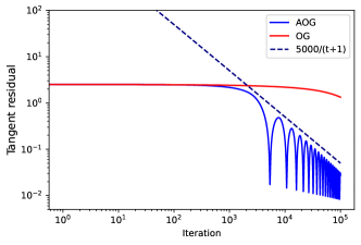
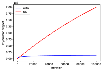
Figure 1: Numerical Results of AOG and OG.

In this section, we numerically verify our theoretical results through Example 1. Let $A\in\mathbbm{R}^{n\times n}$, $b,h\in\mathbbm{R}^{n}$, and $\mathcal{X},\mathcal{Y}\subseteq\mathbbm{R}^{n}$, and $f:\mathcal{X}\times\mathcal{Y}\rightarrow R$ be of the form $f(x,y)=\frac{1}{2}x^{\top}Hx-h^{\top}x-{\mathchoice{\left\langle Ax-b,y\right\rangle}{\langle Ax-b,y\rangle}{\langle Ax-b,y\rangle}{\langle Ax-b,y\rangle}}$ (Ouyang & Xu, 2021). We consider a convex-concave min-max optimization problem $\min_{x\in\mathcal{X}}\max_{y\in\mathcal{Y}}f(x,y)$, which is also a two-player zero-sum game with $f^{1}=-f^{2}=f$. Details of the choices of $H,A,b,h,\mathcal{X},\mathcal{Y}$ and step size $\eta$ are deferred to Appendix F.

The numerical result is shown in Figure 1. We use $\boldsymbol{z}$ to denote $(x,y)$. When players use AOG, the tangent residual of players’ action profile $r^{tan}(\boldsymbol{z}_{t+\frac{1}{2}})$ decreases at a rate of $\mathcal{O}(\frac{1}{T})$, and corroborates our theoretical results (Theorem 2). Moreover, AOG significantly outperforms OG in terms of both the last-iterate convergence rate and the individual dynamic regret.

8 Related Work

Last-Iterate Convergence of No-regret learning in Games

There is a vast literature on no-regret learning in games. For strongly monotone games, linear last-iterate convergence rate is known (Tseng, 1995; Liang & Stokes, 2019; Mokhtari et al., 2020b; Zhou et al., 2020). Even under bandit feedback or noisy gradient feedback, optimal sub-linear last-iterate convergence rate is achieved by no-regret learning algorithms for strongly monotone games (Lin et al., 2022; Jordan et al., 2022).

Obtaining last-iterate convergence rate to Nash equilibria beyond strongly monotone games received extensive attention recently. Daskalakis & Panageas (2018) proved asymptotic convergence of the optimistic gradient (OG) algorithm in zero-sum games. Asymptotic convergence was also achieved in variationally stable games (Zhou et al., 2017b, a; Mertikopoulos & Zhou, 2019; Hsieh et al., 2021) even with noisy feedback (Hsieh et al., 2022). Finite time $\mathcal{O}(\frac{1}{\sqrt{T}})$ convergence was shown for unconstrained cocoercive games (Lin et al., 2020) and unconstrained monotone games (Golowich et al., 2020a). For bilinear games over polytopes, (Wei et al., 2021) show linear convergence rate of OG but this rate depends on a problem constant $c$ which can be arbitrarily large. Recently, Cai et al. (2022b) proved a tight $\mathcal{O}(\frac{1}{\sqrt{T}})$ last-iterate convergence rate of OG and the extragradient (EG) algortihm for constrained monotone games, matching the lower bound of p-SCIL algorithms by Golowich et al. (2020a). We remark that for general gradient-based algorithms, the lower bound is $\Omega(\frac{1}{T})$ (Ouyang & Xu, 2021; Yoon & Ryu, 2021).

Regret Minimization in Games

There is a large collection of works on minimizing individual regret in games, from early results in two-player zero-sum games (Daskalakis et al., 2011; Kangarshahi et al., 2018) to more recent works on general-sum games (Syrgkanis et al., 2015; Chen & Peng, 2020; Daskalakis et al., 2021; Anagnostides et al., 2022a, b). Among them, (Daskalakis et al., 2021; Anagnostides et al., 2022a, b) achieves $\mathcal{O}(\log T)$ regret for general-sum games and (Hsieh et al., 2021) achieves $\mathcal{O}(1)$ regret for variationally stable games. Little is known, however, for the stronger notion of dynamic regret except for $\mathcal{O}(\sqrt{T})$ bound of OG in monotone games (Cai et al., 2022b).

Learning in Repeated Games and Evolutionary Game Theory

Agents in our model could be interpreted as different populations rather than individuals, where the mixed strategy describes the prevalence of each of the pure strategies in the population. Under this interpretation, we no longer have the same players playing the same game every day. Instead, in each round of the repeated game, individuals from one population play the game with other individuals drawn randomly from other populations. Such interpretation has wide application in evolutionary game theory, where repeated games are used to model evolution (see the monograph of (Weibull, 1997) and the references therein for more details).

9 Conclusion and Discussion

In this paper, we propose the first doubly optimal online learning algorithm, the accelerated optimistic gradient (AOG) algorithm, which achieves optimal $\mathcal{O}(\sqrt{T})$ regret bound in the adversarial setting and optimal $\mathcal{O}(\frac{1}{T})$ last-iterate convergence rate in smooth monotone games. Extending our results in settings where players only receive noisy gradient or even bandit feedback is an interesting and challenging future direction. Finally, We significantly improve the state-of-the-art upper bound of the individual dynamic regret from $\mathcal{O}(\sqrt{T})$ to $\mathcal{O}(\log{T})$. We believe that understanding the optimal individual dynamic regret is an interesting open question for learning in monotone games.

Open Question:

What is the optimal individual dynamic regret achievable in smooth monotone games using no-regret learning algorithms?

Acknowledgements

Yang Cai is supported by a Sloan Foundation Research Fellowship and the NSF Award CCF-1942583 (CAREER). We thank the anonymous reviewers for their constructive comments.

Appendix A Missing proofs in Section 3

Proof of Lemma 2: Let us view the update rule of AOG as standard update rule of OG with modified gradients $g_{t-\frac{1}{2}}-\frac{1}{\eta_{t}(t+1)}(x_{1}-x_{t})$ and $g_{t+\frac{1}{2}}-\frac{1}{\eta_{t}(t+1)}(x_{1}-x_{t})$. Thus by the standard analysis of OG (see (Rakhlin & Sridharan, 2013)[Lemma 1]), we have for any $t\geq 1$ and any $x^{\prime}\in\mathcal{X}$,

$${\mathchoice{\left\langle g_{t+\frac{1}{2}}-\frac{1}{\eta_{t}(t+1)}(x_{1}-x_{t}),x_{t+\frac{1}{2}}-x^{\prime}\right\rangle}{\langle g_{t+\frac{1}{2}}-\frac{1}{\eta_{t}(t+1)}(x_{1}-x_{t}),x_{t+\frac{1}{2}}-x^{\prime}\rangle}{\langle g_{t+\frac{1}{2}}-\frac{1}{\eta_{t}(t+1)}(x_{1}-x_{t}),x_{t+\frac{1}{2}}-x^{\prime}\rangle}{\langle g_{t+\frac{1}{2}}-\frac{1}{\eta_{t}(t+1)}(x_{1}-x_{t}),x_{t+\frac{1}{2}}-x^{\prime}\rangle}} \leq\frac{1}{2\eta_{t}}{\mathchoice{\left({\mathchoice{\left\|x_{t}-x^{\prime}\right\|}{\|x_{t}-x^{\prime}\|}{\|x_{t}-x^{\prime}\|}{\|x_{t}-x^{\prime}\|}}^{2}-{\mathchoice{\left\|x_{t+1}-x^{\prime}\right\|}{\|x_{t+1}-x^{\prime}\|}{\|x_{t+1}-x^{\prime}\|}{\|x_{t+1}-x^{\prime}\|}}^{2}\right)}{({\mathchoice{\left\|x_{t}-x^{\prime}\right\|}{\|x_{t}-x^{\prime}\|}{\|x_{t}-x^{\prime}\|}{\|x_{t}-x^{\prime}\|}}^{2}-{\mathchoice{\left\|x_{t+1}-x^{\prime}\right\|}{\|x_{t+1}-x^{\prime}\|}{\|x_{t+1}-x^{\prime}\|}{\|x_{t+1}-x^{\prime}\|}}^{2})}{({\mathchoice{\left\|x_{t}-x^{\prime}\right\|}{\|x_{t}-x^{\prime}\|}{\|x_{t}-x^{\prime}\|}{\|x_{t}-x^{\prime}\|}}^{2}-{\mathchoice{\left\|x_{t+1}-x^{\prime}\right\|}{\|x_{t+1}-x^{\prime}\|}{\|x_{t+1}-x^{\prime}\|}{\|x_{t+1}-x^{\prime}\|}}^{2})}{({\mathchoice{\left\|x_{t}-x^{\prime}\right\|}{\|x_{t}-x^{\prime}\|}{\|x_{t}-x^{\prime}\|}{\|x_{t}-x^{\prime}\|}}^{2}-{\mathchoice{\left\|x_{t+1}-x^{\prime}\right\|}{\|x_{t+1}-x^{\prime}\|}{\|x_{t+1}-x^{\prime}\|}{\|x_{t+1}-x^{\prime}\|}}^{2})}}+{\mathchoice{\left\|g_{t+\frac{1}{2}}-g_{t-\frac{1}{2}}\right\|}{\|g_{t+\frac{1}{2}}-g_{t-\frac{1}{2}}\|}{\|g_{t+\frac{1}{2}}-g_{t-\frac{1}{2}}\|}{\|g_{t+\frac{1}{2}}-g_{t-\frac{1}{2}}\|}}\cdot{\mathchoice{\left\|x_{t+\frac{1}{2}}-x_{t+1}\right\|}{\|x_{t+\frac{1}{2}}-x_{t+1}\|}{\|x_{t+\frac{1}{2}}-x_{t+1}\|}{\|x_{t+\frac{1}{2}}-x_{t+1}\|}}$$

$$\leq\frac{1}{2\eta_{t}}{\mathchoice{\left({\mathchoice{\left\|x_{t}-x^{\prime}\right\|}{\|x_{t}-x^{\prime}\|}{\|x_{t}-x^{\prime}\|}{\|x_{t}-x^{\prime}\|}}^{2}-{\mathchoice{\left\|x_{t+1}-x^{\prime}\right\|}{\|x_{t+1}-x^{\prime}\|}{\|x_{t+1}-x^{\prime}\|}{\|x_{t+1}-x^{\prime}\|}}^{2}\right)}{({\mathchoice{\left\|x_{t}-x^{\prime}\right\|}{\|x_{t}-x^{\prime}\|}{\|x_{t}-x^{\prime}\|}{\|x_{t}-x^{\prime}\|}}^{2}-{\mathchoice{\left\|x_{t+1}-x^{\prime}\right\|}{\|x_{t+1}-x^{\prime}\|}{\|x_{t+1}-x^{\prime}\|}{\|x_{t+1}-x^{\prime}\|}}^{2})}{({\mathchoice{\left\|x_{t}-x^{\prime}\right\|}{\|x_{t}-x^{\prime}\|}{\|x_{t}-x^{\prime}\|}{\|x_{t}-x^{\prime}\|}}^{2}-{\mathchoice{\left\|x_{t+1}-x^{\prime}\right\|}{\|x_{t+1}-x^{\prime}\|}{\|x_{t+1}-x^{\prime}\|}{\|x_{t+1}-x^{\prime}\|}}^{2})}{({\mathchoice{\left\|x_{t}-x^{\prime}\right\|}{\|x_{t}-x^{\prime}\|}{\|x_{t}-x^{\prime}\|}{\|x_{t}-x^{\prime}\|}}^{2}-{\mathchoice{\left\|x_{t+1}-x^{\prime}\right\|}{\|x_{t+1}-x^{\prime}\|}{\|x_{t+1}-x^{\prime}\|}{\|x_{t+1}-x^{\prime}\|}}^{2})}}+\eta_{t}{\mathchoice{\left\|g_{t+\frac{1}{2}}-g_{t-\frac{1}{2}}\right\|}{\|g_{t+\frac{1}{2}}-g_{t-\frac{1}{2}}\|}{\|g_{t+\frac{1}{2}}-g_{t-\frac{1}{2}}\|}{\|g_{t+\frac{1}{2}}-g_{t-\frac{1}{2}}\|}}^{2},$$

where in the second inequality we use the following inequality:

$${\mathchoice{\left\|x_{t+\frac{1}{2}}-x_{t+1}\right\|}{\|x_{t+\frac{1}{2}}-x_{t+1}\|}{\|x_{t+\frac{1}{2}}-x_{t+1}\|}{\|x_{t+\frac{1}{2}}-x_{t+1}\|}} \leq{\mathchoice{\left\|\Pi_{\mathcal{X}}{\mathchoice{\left[x_{t}-\eta_{t}g_{t-\frac{1}{2}}-\frac{1}{t+1}(x_{1}-x_{t})\right]}{[x_{t}-\eta_{t}g_{t-\frac{1}{2}}-\frac{1}{t+1}(x_{1}-x_{t})]}{[x_{t}-\eta_{t}g_{t-\frac{1}{2}}-\frac{1}{t+1}(x_{1}-x_{t})]}{[x_{t}-\eta_{t}g_{t-\frac{1}{2}}-\frac{1}{t+1}(x_{1}-x_{t})]}}-\Pi_{\mathcal{X}}{\mathchoice{\left[x_{t}-\eta_{t}g_{t+\frac{1}{2}}-\frac{1}{t+1}(x_{1}-x_{t})\right]}{[x_{t}-\eta_{t}g_{t+\frac{1}{2}}-\frac{1}{t+1}(x_{1}-x_{t})]}{[x_{t}-\eta_{t}g_{t+\frac{1}{2}}-\frac{1}{t+1}(x_{1}-x_{t})]}{[x_{t}-\eta_{t}g_{t+\frac{1}{2}}-\frac{1}{t+1}(x_{1}-x_{t})]}}\right\|}{\|\Pi_{\mathcal{X}}{\mathchoice{\left[x_{t}-\eta_{t}g_{t-\frac{1}{2}}-\frac{1}{t+1}(x_{1}-x_{t})\right]}{[x_{t}-\eta_{t}g_{t-\frac{1}{2}}-\frac{1}{t+1}(x_{1}-x_{t})]}{[x_{t}-\eta_{t}g_{t-\frac{1}{2}}-\frac{1}{t+1}(x_{1}-x_{t})]}{[x_{t}-\eta_{t}g_{t-\frac{1}{2}}-\frac{1}{t+1}(x_{1}-x_{t})]}}-\Pi_{\mathcal{X}}{\mathchoice{\left[x_{t}-\eta_{t}g_{t+\frac{1}{2}}-\frac{1}{t+1}(x_{1}-x_{t})\right]}{[x_{t}-\eta_{t}g_{t+\frac{1}{2}}-\frac{1}{t+1}(x_{1}-x_{t})]}{[x_{t}-\eta_{t}g_{t+\frac{1}{2}}-\frac{1}{t+1}(x_{1}-x_{t})]}{[x_{t}-\eta_{t}g_{t+\frac{1}{2}}-\frac{1}{t+1}(x_{1}-x_{t})]}}\|}{\|\Pi_{\mathcal{X}}{\mathchoice{\left[x_{t}-\eta_{t}g_{t-\frac{1}{2}}-\frac{1}{t+1}(x_{1}-x_{t})\right]}{[x_{t}-\eta_{t}g_{t-\frac{1}{2}}-\frac{1}{t+1}(x_{1}-x_{t})]}{[x_{t}-\eta_{t}g_{t-\frac{1}{2}}-\frac{1}{t+1}(x_{1}-x_{t})]}{[x_{t}-\eta_{t}g_{t-\frac{1}{2}}-\frac{1}{t+1}(x_{1}-x_{t})]}}-\Pi_{\mathcal{X}}{\mathchoice{\left[x_{t}-\eta_{t}g_{t+\frac{1}{2}}-\frac{1}{t+1}(x_{1}-x_{t})\right]}{[x_{t}-\eta_{t}g_{t+\frac{1}{2}}-\frac{1}{t+1}(x_{1}-x_{t})]}{[x_{t}-\eta_{t}g_{t+\frac{1}{2}}-\frac{1}{t+1}(x_{1}-x_{t})]}{[x_{t}-\eta_{t}g_{t+\frac{1}{2}}-\frac{1}{t+1}(x_{1}-x_{t})]}}\|}{\|\Pi_{\mathcal{X}}{\mathchoice{\left[x_{t}-\eta_{t}g_{t-\frac{1}{2}}-\frac{1}{t+1}(x_{1}-x_{t})\right]}{[x_{t}-\eta_{t}g_{t-\frac{1}{2}}-\frac{1}{t+1}(x_{1}-x_{t})]}{[x_{t}-\eta_{t}g_{t-\frac{1}{2}}-\frac{1}{t+1}(x_{1}-x_{t})]}{[x_{t}-\eta_{t}g_{t-\frac{1}{2}}-\frac{1}{t+1}(x_{1}-x_{t})]}}-\Pi_{\mathcal{X}}{\mathchoice{\left[x_{t}-\eta_{t}g_{t+\frac{1}{2}}-\frac{1}{t+1}(x_{1}-x_{t})\right]}{[x_{t}-\eta_{t}g_{t+\frac{1}{2}}-\frac{1}{t+1}(x_{1}-x_{t})]}{[x_{t}-\eta_{t}g_{t+\frac{1}{2}}-\frac{1}{t+1}(x_{1}-x_{t})]}{[x_{t}-\eta_{t}g_{t+\frac{1}{2}}-\frac{1}{t+1}(x_{1}-x_{t})]}}\|}}$$

$$\leq\eta_{t}{\mathchoice{\left\|g_{t+\frac{1}{2}}-g_{t-\frac{1}{2}}\right\|}{\|g_{t+\frac{1}{2}}-g_{t-\frac{1}{2}}\|}{\|g_{t+\frac{1}{2}}-g_{t-\frac{1}{2}}\|}{\|g_{t+\frac{1}{2}}-g_{t-\frac{1}{2}}\|}}. \Pi_{X}$$ ( is non-expansive)

Therefore, we can bound the single-step regret by

$${\mathchoice{\left\langle g_{t+\frac{1}{2}},x_{t+\frac{1}{2}}-x^{\prime}\right\rangle}{\langle g_{t+\frac{1}{2}},x_{t+\frac{1}{2}}-x^{\prime}\rangle}{\langle g_{t+\frac{1}{2}},x_{t+\frac{1}{2}}-x^{\prime}\rangle}{\langle g_{t+\frac{1}{2}},x_{t+\frac{1}{2}}-x^{\prime}\rangle}} \leq\frac{1}{2\eta_{t}}{\mathchoice{\left({\mathchoice{\left\|x_{t}-x^{\prime}\right\|}{\|x_{t}-x^{\prime}\|}{\|x_{t}-x^{\prime}\|}{\|x_{t}-x^{\prime}\|}}^{2}-{\mathchoice{\left\|x_{t+1}-x^{\prime}\right\|}{\|x_{t+1}-x^{\prime}\|}{\|x_{t+1}-x^{\prime}\|}{\|x_{t+1}-x^{\prime}\|}}^{2}\right)}{({\mathchoice{\left\|x_{t}-x^{\prime}\right\|}{\|x_{t}-x^{\prime}\|}{\|x_{t}-x^{\prime}\|}{\|x_{t}-x^{\prime}\|}}^{2}-{\mathchoice{\left\|x_{t+1}-x^{\prime}\right\|}{\|x_{t+1}-x^{\prime}\|}{\|x_{t+1}-x^{\prime}\|}{\|x_{t+1}-x^{\prime}\|}}^{2})}{({\mathchoice{\left\|x_{t}-x^{\prime}\right\|}{\|x_{t}-x^{\prime}\|}{\|x_{t}-x^{\prime}\|}{\|x_{t}-x^{\prime}\|}}^{2}-{\mathchoice{\left\|x_{t+1}-x^{\prime}\right\|}{\|x_{t+1}-x^{\prime}\|}{\|x_{t+1}-x^{\prime}\|}{\|x_{t+1}-x^{\prime}\|}}^{2})}{({\mathchoice{\left\|x_{t}-x^{\prime}\right\|}{\|x_{t}-x^{\prime}\|}{\|x_{t}-x^{\prime}\|}{\|x_{t}-x^{\prime}\|}}^{2}-{\mathchoice{\left\|x_{t+1}-x^{\prime}\right\|}{\|x_{t+1}-x^{\prime}\|}{\|x_{t+1}-x^{\prime}\|}{\|x_{t+1}-x^{\prime}\|}}^{2})}}+\eta_{t}{\mathchoice{\left\|g_{t+\frac{1}{2}}-g_{t-\frac{1}{2}}\right\|}{\|g_{t+\frac{1}{2}}-g_{t-\frac{1}{2}}\|}{\|g_{t+\frac{1}{2}}-g_{t-\frac{1}{2}}\|}{\|g_{t+\frac{1}{2}}-g_{t-\frac{1}{2}}\|}}^{2}+{\mathchoice{\left\langle\frac{1}{\eta_{t}(t+1)}(x_{1}-x_{t}),x_{t+\frac{1}{2}}-x^{\prime}\right\rangle}{\langle\frac{1}{\eta_{t}(t+1)}(x_{1}-x_{t}),x_{t+\frac{1}{2}}-x^{\prime}\rangle}{\langle\frac{1}{\eta_{t}(t+1)}(x_{1}-x_{t}),x_{t+\frac{1}{2}}-x^{\prime}\rangle}{\langle\frac{1}{\eta_{t}(t+1)}(x_{1}-x_{t}),x_{t+\frac{1}{2}}-x^{\prime}\rangle}}$$

$$\leq\frac{1}{2\eta_{t}}{\mathchoice{\left({\mathchoice{\left\|x_{t}-x^{\prime}\right\|}{\|x_{t}-x^{\prime}\|}{\|x_{t}-x^{\prime}\|}{\|x_{t}-x^{\prime}\|}}^{2}-{\mathchoice{\left\|x_{t+1}-x^{\prime}\right\|}{\|x_{t+1}-x^{\prime}\|}{\|x_{t+1}-x^{\prime}\|}{\|x_{t+1}-x^{\prime}\|}}^{2}\right)}{({\mathchoice{\left\|x_{t}-x^{\prime}\right\|}{\|x_{t}-x^{\prime}\|}{\|x_{t}-x^{\prime}\|}{\|x_{t}-x^{\prime}\|}}^{2}-{\mathchoice{\left\|x_{t+1}-x^{\prime}\right\|}{\|x_{t+1}-x^{\prime}\|}{\|x_{t+1}-x^{\prime}\|}{\|x_{t+1}-x^{\prime}\|}}^{2})}{({\mathchoice{\left\|x_{t}-x^{\prime}\right\|}{\|x_{t}-x^{\prime}\|}{\|x_{t}-x^{\prime}\|}{\|x_{t}-x^{\prime}\|}}^{2}-{\mathchoice{\left\|x_{t+1}-x^{\prime}\right\|}{\|x_{t+1}-x^{\prime}\|}{\|x_{t+1}-x^{\prime}\|}{\|x_{t+1}-x^{\prime}\|}}^{2})}{({\mathchoice{\left\|x_{t}-x^{\prime}\right\|}{\|x_{t}-x^{\prime}\|}{\|x_{t}-x^{\prime}\|}{\|x_{t}-x^{\prime}\|}}^{2}-{\mathchoice{\left\|x_{t+1}-x^{\prime}\right\|}{\|x_{t+1}-x^{\prime}\|}{\|x_{t+1}-x^{\prime}\|}{\|x_{t+1}-x^{\prime}\|}}^{2})}}+\eta_{t}{\mathchoice{\left\|g_{t+\frac{1}{2}}-g_{t-\frac{1}{2}}\right\|}{\|g_{t+\frac{1}{2}}-g_{t-\frac{1}{2}}\|}{\|g_{t+\frac{1}{2}}-g_{t-\frac{1}{2}}\|}{\|g_{t+\frac{1}{2}}-g_{t-\frac{1}{2}}\|}}^{2}+\frac{D^{2}}{\eta_{t}(t+1)},$$

where in the last inequality we use Cauchy-Schwarz inequality and the fact that $\mathcal{X}$ is bounded by $D$. This completes the proof. $\hfill\square$

Proof of Theorem 1: Let $T_{1}\geq 2$ be the last time the player uses constant step size $\eta$. By line 7 of Algorithm 1, we know the the second-order gradient variation $S_{T_{1}+1}\leq S_{T_{1}}+2G^{2}$ is upper bounded by a constant. By telescoping the inequality from Lemma 2, we know that the player’s regret up to time $T_{1}$ is at most

$$\sum_{t=1}^{T_{1}}{\mathchoice{\left\langle g_{t+\frac{1}{2}},x_{t+\frac{1}{2}}-x^{\prime}\right\rangle}{\langle g_{t+\frac{1}{2}},x_{t+\frac{1}{2}}-x^{\prime}\rangle}{\langle g_{t+\frac{1}{2}},x_{t+\frac{1}{2}}-x^{\prime}\rangle}{\langle g_{t+\frac{1}{2}},x_{t+\frac{1}{2}}-x^{\prime}\rangle}}$$

$$\leq\frac{{\mathchoice{\left\|x_{1}-x^{\prime}\right\|}{\|x_{1}-x^{\prime}\|}{\|x_{1}-x^{\prime}\|}{\|x_{1}-x^{\prime}\|}}^{2}}{2\eta}+\eta S_{T_{1}+1}+G^{2}+\sum_{t=1}^{T_{1}}\frac{D^{2}}{\eta(t+1)}$$

$$\leq\mathcal{O}(G^{2}+\log T_{1}).$$

Now we consider $t\geq T_{1}+1$ when the player switches to an adaptive step size. Using Lemma 2, for any $T\geq T_{1}+1$, we have

$$\sum_{t=T_{1}+1}^{T}{\mathchoice{\left\langle g_{t+\frac{1}{2}},x_{t+\frac{1}{2}}-x^{\prime}\right\rangle}{\langle g_{t+\frac{1}{2}},x_{t+\frac{1}{2}}-x^{\prime}\rangle}{\langle g_{t+\frac{1}{2}},x_{t+\frac{1}{2}}-x^{\prime}\rangle}{\langle g_{t+\frac{1}{2}},x_{t+\frac{1}{2}}-x^{\prime}\rangle}}$$

$$\leq\underbrace{\sum_{t=T_{1}+1}^{T}\frac{1}{\eta_{t}}({\mathchoice{\left\|x_{t}-x^{*}\right\|}{\|x_{t}-x^{*}\|}{\|x_{t}-x^{*}\|}{\|x_{t}-x^{*}\|}}^{2}-{\mathchoice{\left\|x_{t+1}-x^{*}\right\|}{\|x_{t+1}-x^{*}\|}{\|x_{t+1}-x^{*}\|}{\|x_{t+1}-x^{*}\|}}^{2})}_{\mathbf{I}}$$

$$\quad\quad+\underbrace{\sum_{t=T_{1}+1}^{T}\eta_{t}{\mathchoice{\left\|g_{t+\frac{1}{2}}-g_{t-\frac{1}{2}}\right\|}{\|g_{t+\frac{1}{2}}-g_{t-\frac{1}{2}}\|}{\|g_{t+\frac{1}{2}}-g_{t-\frac{1}{2}}\|}{\|g_{t+\frac{1}{2}}-g_{t-\frac{1}{2}}\|}}^{2}}_{\mathbf{II}}+\underbrace{\sum_{t=T_{1}+1}^{T}\frac{D^{2}}{\eta_{t}(t+1)}}_{\mathbf{III}}.$$

Since for any $t\geq 1$, ${\mathchoice{\left\|g_{t+\frac{1}{2}}-g_{t-\frac{1}{2}}\right\|}{\|g_{t+\frac{1}{2}}-g_{t-\frac{1}{2}}\|}{\|g_{t+\frac{1}{2}}-g_{t-\frac{1}{2}}\|}{\|g_{t+\frac{1}{2}}-g_{t-\frac{1}{2}}\|}}^{2}\leq 2{\mathchoice{\left\|g_{t+\frac{1}{2}}\right\|}{\|g_{t+\frac{1}{2}}\|}{\|g_{t+\frac{1}{2}}\|}{\|g_{t+\frac{1}{2}}\|}}^{2}+2{\mathchoice{\left\|g_{t-\frac{1}{2}}\right\|}{\|g_{t-\frac{1}{2}}\|}{\|g_{t-\frac{1}{2}}\|}{\|g_{t-\frac{1}{2}}\|}}^{2}\leq 4G^{2}$. We have $S_{t}\leq 4G^{2}t$ and $\eta_{t}=\frac{1}{\sqrt{1+S_{t}}}\geq\frac{1}{2G\sqrt{t}}$ for any $t\geq T_{1}+1$. We now proceed to bound each terms as follows.

$$\mathbf{I}\leq\frac{D^{2}}{\eta_{T_{1}+1}}+\sum_{t=T_{1}+2}^{T}D^{2}{\mathchoice{\left(\frac{1}{\eta_{t}}-\frac{1}{\eta_{t-1}}\right)}{(\frac{1}{\eta_{t}}-\frac{1}{\eta_{t-1}})}{(\frac{1}{\eta_{t}}-\frac{1}{\eta_{t-1}})}{(\frac{1}{\eta_{t}}-\frac{1}{\eta_{t-1}})}}\leq\frac{D^{2}}{\eta_{T}}\leq\mathcal{O}(D^{2}G\sqrt{T}).$$

$$\mathbf{II} =\sum_{t=T_{1}+1}^{T}{\mathchoice{\left(\eta_{t+1}+\eta_{t}-\eta_{t+1}\right)}{(\eta_{t+1}+\eta_{t}-\eta_{t+1})}{(\eta_{t+1}+\eta_{t}-\eta_{t+1})}{(\eta_{t+1}+\eta_{t}-\eta_{t+1})}}{\mathchoice{\left\|g_{t+\frac{1}{2}}-g_{t-\frac{1}{2}}\right\|}{\|g_{t+\frac{1}{2}}-g_{t-\frac{1}{2}}\|}{\|g_{t+\frac{1}{2}}-g_{t-\frac{1}{2}}\|}{\|g_{t+\frac{1}{2}}-g_{t-\frac{1}{2}}\|}}^{2}$$

$$\leq\sum_{t=T_{1}+1}^{T}{\mathchoice{\left(\frac{{\mathchoice{\left\|g_{t+\frac{1}{2}}-g_{t-\frac{1}{2}}\right\|}{\|g_{t+\frac{1}{2}}-g_{t-\frac{1}{2}}\|}{\|g_{t+\frac{1}{2}}-g_{t-\frac{1}{2}}\|}{\|g_{t+\frac{1}{2}}-g_{t-\frac{1}{2}}\|}}^{2}}{\sqrt{1+S_{t+1}}}+4G^{2}(\eta_{t}-\eta_{t+1})\right)}{(\frac{{\mathchoice{\left\|g_{t+\frac{1}{2}}-g_{t-\frac{1}{2}}\right\|}{\|g_{t+\frac{1}{2}}-g_{t-\frac{1}{2}}\|}{\|g_{t+\frac{1}{2}}-g_{t-\frac{1}{2}}\|}{\|g_{t+\frac{1}{2}}-g_{t-\frac{1}{2}}\|}}^{2}}{\sqrt{1+S_{t+1}}}+4G^{2}(\eta_{t}-\eta_{t+1}))}{(\frac{{\mathchoice{\left\|g_{t+\frac{1}{2}}-g_{t-\frac{1}{2}}\right\|}{\|g_{t+\frac{1}{2}}-g_{t-\frac{1}{2}}\|}{\|g_{t+\frac{1}{2}}-g_{t-\frac{1}{2}}\|}{\|g_{t+\frac{1}{2}}-g_{t-\frac{1}{2}}\|}}^{2}}{\sqrt{1+S_{t+1}}}+4G^{2}(\eta_{t}-\eta_{t+1}))}{(\frac{{\mathchoice{\left\|g_{t+\frac{1}{2}}-g_{t-\frac{1}{2}}\right\|}{\|g_{t+\frac{1}{2}}-g_{t-\frac{1}{2}}\|}{\|g_{t+\frac{1}{2}}-g_{t-\frac{1}{2}}\|}{\|g_{t+\frac{1}{2}}-g_{t-\frac{1}{2}}\|}}^{2}}{\sqrt{1+S_{t+1}}}+4G^{2}(\eta_{t}-\eta_{t+1}))}}$$

$$\leq\sum_{t=T_{1}+1}^{T}\frac{(\sqrt{1+S_{t+1}}-\sqrt{1+S_{t}})(\sqrt{1+S_{t+1}}+\sqrt{1+S_{t}})}{\sqrt{1+S_{t+1}}}+4G^{2}$$

$$\leq\sum_{t=T_{1}+1}^{T}2(\sqrt{1+S_{t+1}}-\sqrt{1+S_{t}})+4G^{2}$$

$$\leq 2\sqrt{1+\sum_{t=1}^{T}{\mathchoice{\left\|g_{t+\frac{1}{2}}-g_{t-\frac{1}{2}}\right\|}{\|g_{t+\frac{1}{2}}-g_{t-\frac{1}{2}}\|}{\|g_{t+\frac{1}{2}}-g_{t-\frac{1}{2}}\|}{\|g_{t+\frac{1}{2}}-g_{t-\frac{1}{2}}\|}}^{2}}+4G^{2}=\mathcal{O}(G\sqrt{T}+G^{2}).$$

$$\mathbf{III} \leq D^{2}\sum_{i=1}^{t}\frac{\sqrt{1+S_{t}}}{t+1}\leq D^{2}\sum_{t=1}^{T}\mathcal{O}(\frac{G}{\sqrt{t}})=\mathcal{O}(D^{2}G\sqrt{T}).$$

Combing the above inequalities, we get the regret between $T_{1}$ and $T$ is at most $\mathcal{O}(D^{2}G\sqrt{T}+G^{2})$. $\hfill\square$

Appendix B Missing proofs in Section 5

Proof of Proposition 1: Note that $\boldsymbol{x}_{3/2}=\boldsymbol{x}_{1}$ and $\eta c_{2}=\boldsymbol{x}_{1}-\eta V(\boldsymbol{x}_{1})-\boldsymbol{x}_{2}$. Thus

$${\mathchoice{\left\|\eta V(\boldsymbol{x}_{2})+\eta c_{2}\right\|}{\|\eta V(\boldsymbol{x}_{2})+\eta c_{2}\|}{\|\eta V(\boldsymbol{x}_{2})+\eta c_{2}\|}{\|\eta V(\boldsymbol{x}_{2})+\eta c_{2}\|}} ={\mathchoice{\left\|\eta V(\boldsymbol{x}_{2})+\boldsymbol{x}_{1}-\eta V(\boldsymbol{x}_{1})-\boldsymbol{x}_{2}\right\|}{\|\eta V(\boldsymbol{x}_{2})+\boldsymbol{x}_{1}-\eta V(\boldsymbol{x}_{1})-\boldsymbol{x}_{2}\|}{\|\eta V(\boldsymbol{x}_{2})+\boldsymbol{x}_{1}-\eta V(\boldsymbol{x}_{1})-\boldsymbol{x}_{2}\|}{\|\eta V(\boldsymbol{x}_{2})+\boldsymbol{x}_{1}-\eta V(\boldsymbol{x}_{1})-\boldsymbol{x}_{2}\|}}$$

$$\leq\eta{\mathchoice{\left\|V(\boldsymbol{x}_{2})-V(\boldsymbol{x}_{1})\right\|}{\|V(\boldsymbol{x}_{2})-V(\boldsymbol{x}_{1})\|}{\|V(\boldsymbol{x}_{2})-V(\boldsymbol{x}_{1})\|}{\|V(\boldsymbol{x}_{2})-V(\boldsymbol{x}_{1})\|}}+{\mathchoice{\left\|\boldsymbol{x}_{1}-\boldsymbol{x}_{2}\right\|}{\|\boldsymbol{x}_{1}-\boldsymbol{x}_{2}\|}{\|\boldsymbol{x}_{1}-\boldsymbol{x}_{2}\|}{\|\boldsymbol{x}_{1}-\boldsymbol{x}_{2}\|}}$$

$$\leq(1+\eta L){\mathchoice{\left\|\boldsymbol{x}_{1}-\boldsymbol{x}_{2}\right\|}{\|\boldsymbol{x}_{1}-\boldsymbol{x}_{2}\|}{\|\boldsymbol{x}_{1}-\boldsymbol{x}_{2}\|}{\|\boldsymbol{x}_{1}-\boldsymbol{x}_{2}\|}} V L$$ ( is -Lipschitz)

$$\leq\frac{3D}{2}. \eta L\leq\frac{1}{2}$$ ()

Using the above inequality, we can bound $P_{2}$ as follows:

$$P_{2} =3{\mathchoice{\left({\mathchoice{\left\|\eta V(\boldsymbol{x}_{2})+\eta c_{2}\right\|}{\|\eta V(\boldsymbol{x}_{2})+\eta c_{2}\|}{\|\eta V(\boldsymbol{x}_{2})+\eta c_{2}\|}{\|\eta V(\boldsymbol{x}_{2})+\eta c_{2}\|}}^{2}+{\mathchoice{\left\|\eta V(\boldsymbol{x}_{2})-\eta V(\boldsymbol{x}_{1})\right\|}{\|\eta V(\boldsymbol{x}_{2})-\eta V(\boldsymbol{x}_{1})\|}{\|\eta V(\boldsymbol{x}_{2})-\eta V(\boldsymbol{x}_{1})\|}{\|\eta V(\boldsymbol{x}_{2})-\eta V(\boldsymbol{x}_{1})\|}}^{2}\right)}{({\mathchoice{\left\|\eta V(\boldsymbol{x}_{2})+\eta c_{2}\right\|}{\|\eta V(\boldsymbol{x}_{2})+\eta c_{2}\|}{\|\eta V(\boldsymbol{x}_{2})+\eta c_{2}\|}{\|\eta V(\boldsymbol{x}_{2})+\eta c_{2}\|}}^{2}+{\mathchoice{\left\|\eta V(\boldsymbol{x}_{2})-\eta V(\boldsymbol{x}_{1})\right\|}{\|\eta V(\boldsymbol{x}_{2})-\eta V(\boldsymbol{x}_{1})\|}{\|\eta V(\boldsymbol{x}_{2})-\eta V(\boldsymbol{x}_{1})\|}{\|\eta V(\boldsymbol{x}_{2})-\eta V(\boldsymbol{x}_{1})\|}}^{2})}{({\mathchoice{\left\|\eta V(\boldsymbol{x}_{2})+\eta c_{2}\right\|}{\|\eta V(\boldsymbol{x}_{2})+\eta c_{2}\|}{\|\eta V(\boldsymbol{x}_{2})+\eta c_{2}\|}{\|\eta V(\boldsymbol{x}_{2})+\eta c_{2}\|}}^{2}+{\mathchoice{\left\|\eta V(\boldsymbol{x}_{2})-\eta V(\boldsymbol{x}_{1})\right\|}{\|\eta V(\boldsymbol{x}_{2})-\eta V(\boldsymbol{x}_{1})\|}{\|\eta V(\boldsymbol{x}_{2})-\eta V(\boldsymbol{x}_{1})\|}{\|\eta V(\boldsymbol{x}_{2})-\eta V(\boldsymbol{x}_{1})\|}}^{2})}{({\mathchoice{\left\|\eta V(\boldsymbol{x}_{2})+\eta c_{2}\right\|}{\|\eta V(\boldsymbol{x}_{2})+\eta c_{2}\|}{\|\eta V(\boldsymbol{x}_{2})+\eta c_{2}\|}{\|\eta V(\boldsymbol{x}_{2})+\eta c_{2}\|}}^{2}+{\mathchoice{\left\|\eta V(\boldsymbol{x}_{2})-\eta V(\boldsymbol{x}_{1})\right\|}{\|\eta V(\boldsymbol{x}_{2})-\eta V(\boldsymbol{x}_{1})\|}{\|\eta V(\boldsymbol{x}_{2})-\eta V(\boldsymbol{x}_{1})\|}{\|\eta V(\boldsymbol{x}_{2})-\eta V(\boldsymbol{x}_{1})\|}}^{2})}}+2{\mathchoice{\left\langle\eta V(\boldsymbol{x}_{2})+\eta c_{2},\boldsymbol{x}_{2}-\boldsymbol{x}_{1}\right\rangle}{\langle\eta V(\boldsymbol{x}_{2})+\eta c_{2},\boldsymbol{x}_{2}-\boldsymbol{x}_{1}\rangle}{\langle\eta V(\boldsymbol{x}_{2})+\eta c_{2},\boldsymbol{x}_{2}-\boldsymbol{x}_{1}\rangle}{\langle\eta V(\boldsymbol{x}_{2})+\eta c_{2},\boldsymbol{x}_{2}-\boldsymbol{x}_{1}\rangle}}$$

$$\leq 3{\mathchoice{\left({\mathchoice{\left\|\eta V(\boldsymbol{x}_{2})+\eta c_{2}\right\|}{\|\eta V(\boldsymbol{x}_{2})+\eta c_{2}\|}{\|\eta V(\boldsymbol{x}_{2})+\eta c_{2}\|}{\|\eta V(\boldsymbol{x}_{2})+\eta c_{2}\|}}^{2}+\eta L{\mathchoice{\left\|\boldsymbol{x}_{2}-\boldsymbol{x}_{1}\right\|}{\|\boldsymbol{x}_{2}-\boldsymbol{x}_{1}\|}{\|\boldsymbol{x}_{2}-\boldsymbol{x}_{1}\|}{\|\boldsymbol{x}_{2}-\boldsymbol{x}_{1}\|}}^{2}\right)}{({\mathchoice{\left\|\eta V(\boldsymbol{x}_{2})+\eta c_{2}\right\|}{\|\eta V(\boldsymbol{x}_{2})+\eta c_{2}\|}{\|\eta V(\boldsymbol{x}_{2})+\eta c_{2}\|}{\|\eta V(\boldsymbol{x}_{2})+\eta c_{2}\|}}^{2}+\eta L{\mathchoice{\left\|\boldsymbol{x}_{2}-\boldsymbol{x}_{1}\right\|}{\|\boldsymbol{x}_{2}-\boldsymbol{x}_{1}\|}{\|\boldsymbol{x}_{2}-\boldsymbol{x}_{1}\|}{\|\boldsymbol{x}_{2}-\boldsymbol{x}_{1}\|}}^{2})}{({\mathchoice{\left\|\eta V(\boldsymbol{x}_{2})+\eta c_{2}\right\|}{\|\eta V(\boldsymbol{x}_{2})+\eta c_{2}\|}{\|\eta V(\boldsymbol{x}_{2})+\eta c_{2}\|}{\|\eta V(\boldsymbol{x}_{2})+\eta c_{2}\|}}^{2}+\eta L{\mathchoice{\left\|\boldsymbol{x}_{2}-\boldsymbol{x}_{1}\right\|}{\|\boldsymbol{x}_{2}-\boldsymbol{x}_{1}\|}{\|\boldsymbol{x}_{2}-\boldsymbol{x}_{1}\|}{\|\boldsymbol{x}_{2}-\boldsymbol{x}_{1}\|}}^{2})}{({\mathchoice{\left\|\eta V(\boldsymbol{x}_{2})+\eta c_{2}\right\|}{\|\eta V(\boldsymbol{x}_{2})+\eta c_{2}\|}{\|\eta V(\boldsymbol{x}_{2})+\eta c_{2}\|}{\|\eta V(\boldsymbol{x}_{2})+\eta c_{2}\|}}^{2}+\eta L{\mathchoice{\left\|\boldsymbol{x}_{2}-\boldsymbol{x}_{1}\right\|}{\|\boldsymbol{x}_{2}-\boldsymbol{x}_{1}\|}{\|\boldsymbol{x}_{2}-\boldsymbol{x}_{1}\|}{\|\boldsymbol{x}_{2}-\boldsymbol{x}_{1}\|}}^{2})}}+2{\mathchoice{\left\|\eta V(\boldsymbol{x}_{2})+\eta c_{2}\right\|}{\|\eta V(\boldsymbol{x}_{2})+\eta c_{2}\|}{\|\eta V(\boldsymbol{x}_{2})+\eta c_{2}\|}{\|\eta V(\boldsymbol{x}_{2})+\eta c_{2}\|}}{\mathchoice{\left\|\boldsymbol{x}_{2}-\boldsymbol{x}_{1}\right\|}{\|\boldsymbol{x}_{2}-\boldsymbol{x}_{1}\|}{\|\boldsymbol{x}_{2}-\boldsymbol{x}_{1}\|}{\|\boldsymbol{x}_{2}-\boldsymbol{x}_{1}\|}}$$

$$\leq 3{\mathchoice{\left(\frac{9D^{2}}{4}+\frac{D^{2}}{4}\right)}{(\frac{9D^{2}}{4}+\frac{D^{2}}{4})}{(\frac{9D^{2}}{4}+\frac{D^{2}}{4})}{(\frac{9D^{2}}{4}+\frac{D^{2}}{4})}}+3D^{2} \eta L\leq\frac{1}{2}$$ ()

$$=\frac{33D^{2}}{4}\leq 9D^{2}.$$

This completes the proof of Proposition 1. $\hfill\square$

Proof of Lemma 5: Fix any $t\geq 2$. Using triangle inequality, we have

$${\mathchoice{\left\|\boldsymbol{x}_{t+\frac{1}{2}}-\boldsymbol{x}_{t}\right\|}{\|\boldsymbol{x}_{t+\frac{1}{2}}-\boldsymbol{x}_{t}\|}{\|\boldsymbol{x}_{t+\frac{1}{2}}-\boldsymbol{x}_{t}\|}{\|\boldsymbol{x}_{t+\frac{1}{2}}-\boldsymbol{x}_{t}\|}}\leq{\mathchoice{\left\|\boldsymbol{x}_{t+\frac{1}{2}}-\Pi_{\mathcal{X}}{\mathchoice{\left[\boldsymbol{x}_{t}-\eta V(\boldsymbol{x}_{t})\right]}{[\boldsymbol{x}_{t}-\eta V(\boldsymbol{x}_{t})]}{[\boldsymbol{x}_{t}-\eta V(\boldsymbol{x}_{t})]}{[\boldsymbol{x}_{t}-\eta V(\boldsymbol{x}_{t})]}}\right\|}{\|\boldsymbol{x}_{t+\frac{1}{2}}-\Pi_{\mathcal{X}}{\mathchoice{\left[\boldsymbol{x}_{t}-\eta V(\boldsymbol{x}_{t})\right]}{[\boldsymbol{x}_{t}-\eta V(\boldsymbol{x}_{t})]}{[\boldsymbol{x}_{t}-\eta V(\boldsymbol{x}_{t})]}{[\boldsymbol{x}_{t}-\eta V(\boldsymbol{x}_{t})]}}\|}{\|\boldsymbol{x}_{t+\frac{1}{2}}-\Pi_{\mathcal{X}}{\mathchoice{\left[\boldsymbol{x}_{t}-\eta V(\boldsymbol{x}_{t})\right]}{[\boldsymbol{x}_{t}-\eta V(\boldsymbol{x}_{t})]}{[\boldsymbol{x}_{t}-\eta V(\boldsymbol{x}_{t})]}{[\boldsymbol{x}_{t}-\eta V(\boldsymbol{x}_{t})]}}\|}{\|\boldsymbol{x}_{t+\frac{1}{2}}-\Pi_{\mathcal{X}}{\mathchoice{\left[\boldsymbol{x}_{t}-\eta V(\boldsymbol{x}_{t})\right]}{[\boldsymbol{x}_{t}-\eta V(\boldsymbol{x}_{t})]}{[\boldsymbol{x}_{t}-\eta V(\boldsymbol{x}_{t})]}{[\boldsymbol{x}_{t}-\eta V(\boldsymbol{x}_{t})]}}\|}}+{\mathchoice{\left\|\Pi_{\mathcal{X}}{\mathchoice{\left[\boldsymbol{x}_{t}-\eta V(\boldsymbol{x}_{t})\right]}{[\boldsymbol{x}_{t}-\eta V(\boldsymbol{x}_{t})]}{[\boldsymbol{x}_{t}-\eta V(\boldsymbol{x}_{t})]}{[\boldsymbol{x}_{t}-\eta V(\boldsymbol{x}_{t})]}}-\boldsymbol{x}_{t}\right\|}{\|\Pi_{\mathcal{X}}{\mathchoice{\left[\boldsymbol{x}_{t}-\eta V(\boldsymbol{x}_{t})\right]}{[\boldsymbol{x}_{t}-\eta V(\boldsymbol{x}_{t})]}{[\boldsymbol{x}_{t}-\eta V(\boldsymbol{x}_{t})]}{[\boldsymbol{x}_{t}-\eta V(\boldsymbol{x}_{t})]}}-\boldsymbol{x}_{t}\|}{\|\Pi_{\mathcal{X}}{\mathchoice{\left[\boldsymbol{x}_{t}-\eta V(\boldsymbol{x}_{t})\right]}{[\boldsymbol{x}_{t}-\eta V(\boldsymbol{x}_{t})]}{[\boldsymbol{x}_{t}-\eta V(\boldsymbol{x}_{t})]}{[\boldsymbol{x}_{t}-\eta V(\boldsymbol{x}_{t})]}}-\boldsymbol{x}_{t}\|}{\|\Pi_{\mathcal{X}}{\mathchoice{\left[\boldsymbol{x}_{t}-\eta V(\boldsymbol{x}_{t})\right]}{[\boldsymbol{x}_{t}-\eta V(\boldsymbol{x}_{t})]}{[\boldsymbol{x}_{t}-\eta V(\boldsymbol{x}_{t})]}{[\boldsymbol{x}_{t}-\eta V(\boldsymbol{x}_{t})]}}-\boldsymbol{x}_{t}\|}}.$$

We can bound the first term as follows:

$${\mathchoice{\left\|\boldsymbol{x}_{t+\frac{1}{2}}-\Pi_{\mathcal{X}}{\mathchoice{\left[\boldsymbol{x}_{t}-\eta V(\boldsymbol{x}_{t})\right]}{[\boldsymbol{x}_{t}-\eta V(\boldsymbol{x}_{t})]}{[\boldsymbol{x}_{t}-\eta V(\boldsymbol{x}_{t})]}{[\boldsymbol{x}_{t}-\eta V(\boldsymbol{x}_{t})]}}\right\|}{\|\boldsymbol{x}_{t+\frac{1}{2}}-\Pi_{\mathcal{X}}{\mathchoice{\left[\boldsymbol{x}_{t}-\eta V(\boldsymbol{x}_{t})\right]}{[\boldsymbol{x}_{t}-\eta V(\boldsymbol{x}_{t})]}{[\boldsymbol{x}_{t}-\eta V(\boldsymbol{x}_{t})]}{[\boldsymbol{x}_{t}-\eta V(\boldsymbol{x}_{t})]}}\|}{\|\boldsymbol{x}_{t+\frac{1}{2}}-\Pi_{\mathcal{X}}{\mathchoice{\left[\boldsymbol{x}_{t}-\eta V(\boldsymbol{x}_{t})\right]}{[\boldsymbol{x}_{t}-\eta V(\boldsymbol{x}_{t})]}{[\boldsymbol{x}_{t}-\eta V(\boldsymbol{x}_{t})]}{[\boldsymbol{x}_{t}-\eta V(\boldsymbol{x}_{t})]}}\|}{\|\boldsymbol{x}_{t+\frac{1}{2}}-\Pi_{\mathcal{X}}{\mathchoice{\left[\boldsymbol{x}_{t}-\eta V(\boldsymbol{x}_{t})\right]}{[\boldsymbol{x}_{t}-\eta V(\boldsymbol{x}_{t})]}{[\boldsymbol{x}_{t}-\eta V(\boldsymbol{x}_{t})]}{[\boldsymbol{x}_{t}-\eta V(\boldsymbol{x}_{t})]}}\|}} ={\mathchoice{\left\|\Pi_{\mathcal{X}}{\mathchoice{\left[\boldsymbol{x}_{t}-\eta V(\boldsymbol{x}_{t-\frac{1}{2}})+\frac{1}{t+1}(\boldsymbol{x}_{1}-\boldsymbol{x}_{t})\right]}{[\boldsymbol{x}_{t}-\eta V(\boldsymbol{x}_{t-\frac{1}{2}})+\frac{1}{t+1}(\boldsymbol{x}_{1}-\boldsymbol{x}_{t})]}{[\boldsymbol{x}_{t}-\eta V(\boldsymbol{x}_{t-\frac{1}{2}})+\frac{1}{t+1}(\boldsymbol{x}_{1}-\boldsymbol{x}_{t})]}{[\boldsymbol{x}_{t}-\eta V(\boldsymbol{x}_{t-\frac{1}{2}})+\frac{1}{t+1}(\boldsymbol{x}_{1}-\boldsymbol{x}_{t})]}}-\Pi_{\mathcal{X}}{\mathchoice{\left[\boldsymbol{x}_{t}-\eta V(\boldsymbol{x}_{t})\right]}{[\boldsymbol{x}_{t}-\eta V(\boldsymbol{x}_{t})]}{[\boldsymbol{x}_{t}-\eta V(\boldsymbol{x}_{t})]}{[\boldsymbol{x}_{t}-\eta V(\boldsymbol{x}_{t})]}}\right\|}{\|\Pi_{\mathcal{X}}{\mathchoice{\left[\boldsymbol{x}_{t}-\eta V(\boldsymbol{x}_{t-\frac{1}{2}})+\frac{1}{t+1}(\boldsymbol{x}_{1}-\boldsymbol{x}_{t})\right]}{[\boldsymbol{x}_{t}-\eta V(\boldsymbol{x}_{t-\frac{1}{2}})+\frac{1}{t+1}(\boldsymbol{x}_{1}-\boldsymbol{x}_{t})]}{[\boldsymbol{x}_{t}-\eta V(\boldsymbol{x}_{t-\frac{1}{2}})+\frac{1}{t+1}(\boldsymbol{x}_{1}-\boldsymbol{x}_{t})]}{[\boldsymbol{x}_{t}-\eta V(\boldsymbol{x}_{t-\frac{1}{2}})+\frac{1}{t+1}(\boldsymbol{x}_{1}-\boldsymbol{x}_{t})]}}-\Pi_{\mathcal{X}}{\mathchoice{\left[\boldsymbol{x}_{t}-\eta V(\boldsymbol{x}_{t})\right]}{[\boldsymbol{x}_{t}-\eta V(\boldsymbol{x}_{t})]}{[\boldsymbol{x}_{t}-\eta V(\boldsymbol{x}_{t})]}{[\boldsymbol{x}_{t}-\eta V(\boldsymbol{x}_{t})]}}\|}{\|\Pi_{\mathcal{X}}{\mathchoice{\left[\boldsymbol{x}_{t}-\eta V(\boldsymbol{x}_{t-\frac{1}{2}})+\frac{1}{t+1}(\boldsymbol{x}_{1}-\boldsymbol{x}_{t})\right]}{[\boldsymbol{x}_{t}-\eta V(\boldsymbol{x}_{t-\frac{1}{2}})+\frac{1}{t+1}(\boldsymbol{x}_{1}-\boldsymbol{x}_{t})]}{[\boldsymbol{x}_{t}-\eta V(\boldsymbol{x}_{t-\frac{1}{2}})+\frac{1}{t+1}(\boldsymbol{x}_{1}-\boldsymbol{x}_{t})]}{[\boldsymbol{x}_{t}-\eta V(\boldsymbol{x}_{t-\frac{1}{2}})+\frac{1}{t+1}(\boldsymbol{x}_{1}-\boldsymbol{x}_{t})]}}-\Pi_{\mathcal{X}}{\mathchoice{\left[\boldsymbol{x}_{t}-\eta V(\boldsymbol{x}_{t})\right]}{[\boldsymbol{x}_{t}-\eta V(\boldsymbol{x}_{t})]}{[\boldsymbol{x}_{t}-\eta V(\boldsymbol{x}_{t})]}{[\boldsymbol{x}_{t}-\eta V(\boldsymbol{x}_{t})]}}\|}{\|\Pi_{\mathcal{X}}{\mathchoice{\left[\boldsymbol{x}_{t}-\eta V(\boldsymbol{x}_{t-\frac{1}{2}})+\frac{1}{t+1}(\boldsymbol{x}_{1}-\boldsymbol{x}_{t})\right]}{[\boldsymbol{x}_{t}-\eta V(\boldsymbol{x}_{t-\frac{1}{2}})+\frac{1}{t+1}(\boldsymbol{x}_{1}-\boldsymbol{x}_{t})]}{[\boldsymbol{x}_{t}-\eta V(\boldsymbol{x}_{t-\frac{1}{2}})+\frac{1}{t+1}(\boldsymbol{x}_{1}-\boldsymbol{x}_{t})]}{[\boldsymbol{x}_{t}-\eta V(\boldsymbol{x}_{t-\frac{1}{2}})+\frac{1}{t+1}(\boldsymbol{x}_{1}-\boldsymbol{x}_{t})]}}-\Pi_{\mathcal{X}}{\mathchoice{\left[\boldsymbol{x}_{t}-\eta V(\boldsymbol{x}_{t})\right]}{[\boldsymbol{x}_{t}-\eta V(\boldsymbol{x}_{t})]}{[\boldsymbol{x}_{t}-\eta V(\boldsymbol{x}_{t})]}{[\boldsymbol{x}_{t}-\eta V(\boldsymbol{x}_{t})]}}\|}}$$

$$\leq{\mathchoice{\left\|\eta V(\boldsymbol{x}_{t})-\eta V(\boldsymbol{x}_{t-\frac{1}{2}})+\frac{1}{t+1}(\boldsymbol{x}_{1}-\boldsymbol{x}_{t})\right\|}{\|\eta V(\boldsymbol{x}_{t})-\eta V(\boldsymbol{x}_{t-\frac{1}{2}})+\frac{1}{t+1}(\boldsymbol{x}_{1}-\boldsymbol{x}_{t})\|}{\|\eta V(\boldsymbol{x}_{t})-\eta V(\boldsymbol{x}_{t-\frac{1}{2}})+\frac{1}{t+1}(\boldsymbol{x}_{1}-\boldsymbol{x}_{t})\|}{\|\eta V(\boldsymbol{x}_{t})-\eta V(\boldsymbol{x}_{t-\frac{1}{2}})+\frac{1}{t+1}(\boldsymbol{x}_{1}-\boldsymbol{x}_{t})\|}} \Pi_{X}$$ ( is non-expansive)

$$\leq{\mathchoice{\left\|\eta V(\boldsymbol{x}_{t})-\eta V(\boldsymbol{x}_{t-\frac{1}{2}})\right\|}{\|\eta V(\boldsymbol{x}_{t})-\eta V(\boldsymbol{x}_{t-\frac{1}{2}})\|}{\|\eta V(\boldsymbol{x}_{t})-\eta V(\boldsymbol{x}_{t-\frac{1}{2}})\|}{\|\eta V(\boldsymbol{x}_{t})-\eta V(\boldsymbol{x}_{t-\frac{1}{2}})\|}}+\frac{{\mathchoice{\left\|\boldsymbol{x}_{1}-\boldsymbol{x}_{t}\right\|}{\|\boldsymbol{x}_{1}-\boldsymbol{x}_{t}\|}{\|\boldsymbol{x}_{1}-\boldsymbol{x}_{t}\|}{\|\boldsymbol{x}_{1}-\boldsymbol{x}_{t}\|}}}{t+1}$$

$$\leq\frac{14D}{t}.$$ (Lemma 4)

Since $c_{t}\in N_{\mathcal{X}}(\boldsymbol{x}_{t})$, we have $\boldsymbol{x}_{t}=\Pi_{\mathcal{X}}{\mathchoice{\left[\boldsymbol{x}_{t}+\eta c_{t}\right]}{[\boldsymbol{x}_{t}+\eta c_{t}]}{[\boldsymbol{x}_{t}+\eta c_{t}]}{[\boldsymbol{x}_{t}+\eta c_{t}]}}$. Using this fact we can bound the second term:

$${\mathchoice{\left\|\Pi_{\mathcal{X}}{\mathchoice{\left[\boldsymbol{x}_{t}-\eta V(\boldsymbol{x}_{t})\right]}{[\boldsymbol{x}_{t}-\eta V(\boldsymbol{x}_{t})]}{[\boldsymbol{x}_{t}-\eta V(\boldsymbol{x}_{t})]}{[\boldsymbol{x}_{t}-\eta V(\boldsymbol{x}_{t})]}}-\boldsymbol{x}_{t}\right\|}{\|\Pi_{\mathcal{X}}{\mathchoice{\left[\boldsymbol{x}_{t}-\eta V(\boldsymbol{x}_{t})\right]}{[\boldsymbol{x}_{t}-\eta V(\boldsymbol{x}_{t})]}{[\boldsymbol{x}_{t}-\eta V(\boldsymbol{x}_{t})]}{[\boldsymbol{x}_{t}-\eta V(\boldsymbol{x}_{t})]}}-\boldsymbol{x}_{t}\|}{\|\Pi_{\mathcal{X}}{\mathchoice{\left[\boldsymbol{x}_{t}-\eta V(\boldsymbol{x}_{t})\right]}{[\boldsymbol{x}_{t}-\eta V(\boldsymbol{x}_{t})]}{[\boldsymbol{x}_{t}-\eta V(\boldsymbol{x}_{t})]}{[\boldsymbol{x}_{t}-\eta V(\boldsymbol{x}_{t})]}}-\boldsymbol{x}_{t}\|}{\|\Pi_{\mathcal{X}}{\mathchoice{\left[\boldsymbol{x}_{t}-\eta V(\boldsymbol{x}_{t})\right]}{[\boldsymbol{x}_{t}-\eta V(\boldsymbol{x}_{t})]}{[\boldsymbol{x}_{t}-\eta V(\boldsymbol{x}_{t})]}{[\boldsymbol{x}_{t}-\eta V(\boldsymbol{x}_{t})]}}-\boldsymbol{x}_{t}\|}} ={\mathchoice{\left\|\Pi_{\mathcal{X}}{\mathchoice{\left[\boldsymbol{x}_{t}-\eta V(\boldsymbol{x}_{t})\right]}{[\boldsymbol{x}_{t}-\eta V(\boldsymbol{x}_{t})]}{[\boldsymbol{x}_{t}-\eta V(\boldsymbol{x}_{t})]}{[\boldsymbol{x}_{t}-\eta V(\boldsymbol{x}_{t})]}}-\Pi_{\mathcal{X}}{\mathchoice{\left[\boldsymbol{x}_{t}+\eta c_{t}\right]}{[\boldsymbol{x}_{t}+\eta c_{t}]}{[\boldsymbol{x}_{t}+\eta c_{t}]}{[\boldsymbol{x}_{t}+\eta c_{t}]}}\right\|}{\|\Pi_{\mathcal{X}}{\mathchoice{\left[\boldsymbol{x}_{t}-\eta V(\boldsymbol{x}_{t})\right]}{[\boldsymbol{x}_{t}-\eta V(\boldsymbol{x}_{t})]}{[\boldsymbol{x}_{t}-\eta V(\boldsymbol{x}_{t})]}{[\boldsymbol{x}_{t}-\eta V(\boldsymbol{x}_{t})]}}-\Pi_{\mathcal{X}}{\mathchoice{\left[\boldsymbol{x}_{t}+\eta c_{t}\right]}{[\boldsymbol{x}_{t}+\eta c_{t}]}{[\boldsymbol{x}_{t}+\eta c_{t}]}{[\boldsymbol{x}_{t}+\eta c_{t}]}}\|}{\|\Pi_{\mathcal{X}}{\mathchoice{\left[\boldsymbol{x}_{t}-\eta V(\boldsymbol{x}_{t})\right]}{[\boldsymbol{x}_{t}-\eta V(\boldsymbol{x}_{t})]}{[\boldsymbol{x}_{t}-\eta V(\boldsymbol{x}_{t})]}{[\boldsymbol{x}_{t}-\eta V(\boldsymbol{x}_{t})]}}-\Pi_{\mathcal{X}}{\mathchoice{\left[\boldsymbol{x}_{t}+\eta c_{t}\right]}{[\boldsymbol{x}_{t}+\eta c_{t}]}{[\boldsymbol{x}_{t}+\eta c_{t}]}{[\boldsymbol{x}_{t}+\eta c_{t}]}}\|}{\|\Pi_{\mathcal{X}}{\mathchoice{\left[\boldsymbol{x}_{t}-\eta V(\boldsymbol{x}_{t})\right]}{[\boldsymbol{x}_{t}-\eta V(\boldsymbol{x}_{t})]}{[\boldsymbol{x}_{t}-\eta V(\boldsymbol{x}_{t})]}{[\boldsymbol{x}_{t}-\eta V(\boldsymbol{x}_{t})]}}-\Pi_{\mathcal{X}}{\mathchoice{\left[\boldsymbol{x}_{t}+\eta c_{t}\right]}{[\boldsymbol{x}_{t}+\eta c_{t}]}{[\boldsymbol{x}_{t}+\eta c_{t}]}{[\boldsymbol{x}_{t}+\eta c_{t}]}}\|}}$$

$$\leq{\mathchoice{\left\|\eta V(\boldsymbol{x}_{t})+\eta c_{t}\right\|}{\|\eta V(\boldsymbol{x}_{t})+\eta c_{t}\|}{\|\eta V(\boldsymbol{x}_{t})+\eta c_{t}\|}{\|\eta V(\boldsymbol{x}_{t})+\eta c_{t}\|}} \Pi_{X}$$ ( is non-expansive)

$$\leq\frac{13D}{t}.$$ (Lemma 4)

Combing the above inequalities, we have ${\mathchoice{\left\|\boldsymbol{x}_{t+\frac{1}{2}}-\boldsymbol{x}_{t}\right\|}{\|\boldsymbol{x}_{t+\frac{1}{2}}-\boldsymbol{x}_{t}\|}{\|\boldsymbol{x}_{t+\frac{1}{2}}-\boldsymbol{x}_{t}\|}{\|\boldsymbol{x}_{t+\frac{1}{2}}-\boldsymbol{x}_{t}\|}}\leq\frac{27D}{t}$. This completes the proof of Lemma 5. $\hfill\square$

Appendix C Last-Iterate Convergence Rate without the Boundedness Assumption

Recall that we prove $r^{tan}(\boldsymbol{x}_{T+\frac{1}{2}})\leq\frac{55D}{\eta T}$ for all $T\geq 2$ in Theorem 2 with the assumption that the action set $\mathcal{X}$ is bounded by $D>0$. In this section, we prove last-iterate convergence rate of AOG, which is similar to Theorem 2 but without the boundedness assumption on $\mathcal{X}$.

Theorem 6.

Let $\mathcal{G}=\{N,(\mathcal{X}^{i})_{i\in[N]},(\ell^{i})_{i\in[N]}\}$ be a $L$-smooth monotone game, where each player $i$’s action set $\mathcal{X}^{i}\subseteq\mathbbm{R}^{n_{i}}$ is convex and closed, but not necessarily compact. When all players employ AOG with a constant step size $\eta\leq\frac{1}{\sqrt{6}L}$ in $\mathcal{G}$, then for any $T\geq 2$, we have

$$r^{tan}(\boldsymbol{x}_{T+\frac{1}{2}})\leq\frac{1430H}{\eta T},$$

where $H=\max\{\eta\cdot r^{tan}(\boldsymbol{x}_{1}),{\mathchoice{\left\|\boldsymbol{x}_{1}-\boldsymbol{x}_{\star}\right\|}{\|\boldsymbol{x}_{1}-\boldsymbol{x}_{\star}\|}{\|\boldsymbol{x}_{1}-\boldsymbol{x}_{\star}\|}{\|\boldsymbol{x}_{1}-\boldsymbol{x}_{\star}\|}}\}$ with $\boldsymbol{x}_{\star}$ being an Nash equilibrium of $\mathcal{G}$.

Proof.

We will go through the proof of the first part of Theorem 2 (including Proposition 1, Lemma 4, and Lemma 5), check every application of the boundedness assumption, and give upper bound on these terms using $H$.

In the proof of Proposition 1, the boundedness assumption is used to bound ${\mathchoice{\left\|\boldsymbol{x}_{1}-\boldsymbol{x}_{2}\right\|}{\|\boldsymbol{x}_{1}-\boldsymbol{x}_{2}\|}{\|\boldsymbol{x}_{1}-\boldsymbol{x}_{2}\|}{\|\boldsymbol{x}_{1}-\boldsymbol{x}_{2}\|}}$. Here we show that it is upper bounded by $H$. Let $c\in N_{\mathcal{X}}(\boldsymbol{x}_{1})$ be any vector in the normal cone $N_{\mathcal{X}}(\boldsymbol{x})$. Then we have

$${\mathchoice{\left\|\boldsymbol{x}_{1}-\boldsymbol{x}_{2}\right\|}{\|\boldsymbol{x}_{1}-\boldsymbol{x}_{2}\|}{\|\boldsymbol{x}_{1}-\boldsymbol{x}_{2}\|}{\|\boldsymbol{x}_{1}-\boldsymbol{x}_{2}\|}}\leq{\mathchoice{\left\|\Pi_{\mathcal{X}}[\boldsymbol{x}_{1}-\eta c]\right\|}{\|\Pi_{\mathcal{X}}[\boldsymbol{x}_{1}-\eta c]\|}{\|\Pi_{\mathcal{X}}[\boldsymbol{x}_{1}-\eta c]\|}{\|\Pi_{\mathcal{X}}[\boldsymbol{x}_{1}-\eta c]\|}}-\Pi_{\mathcal{X}}[\boldsymbol{x}_{1}-\eta V(\boldsymbol{x}_{1})]\leq\eta{\mathchoice{\left\|V(\boldsymbol{x}_{1})+c\right\|}{\|V(\boldsymbol{x}_{1})+c\|}{\|V(\boldsymbol{x}_{1})+c\|}{\|V(\boldsymbol{x}_{1})+c\|}}.$$

Thus ${\mathchoice{\left\|\boldsymbol{x}_{1}-\boldsymbol{x}_{2}\right\|}{\|\boldsymbol{x}_{1}-\boldsymbol{x}_{2}\|}{\|\boldsymbol{x}_{1}-\boldsymbol{x}_{2}\|}{\|\boldsymbol{x}_{1}-\boldsymbol{x}_{2}\|}}\leq\eta\cdot r^{tan}(\boldsymbol{x}_{1})\leq H$.

In the proof of Lemma 4, the boundedness assumption is applied to bound ${\mathchoice{\left\|\boldsymbol{x}_{1}-\boldsymbol{x}_{\star}\right\|}{\|\boldsymbol{x}_{1}-\boldsymbol{x}_{\star}\|}{\|\boldsymbol{x}_{1}-\boldsymbol{x}_{\star}\|}{\|\boldsymbol{x}_{1}-\boldsymbol{x}_{\star}\|}}$, which is clearly upper bounded by $H$. Combing the above two observations, we get a modified version of Lemma 4 (replacing $D$ with $H$): for all $t\geq 2$,

$${\mathchoice{\left\|V(\boldsymbol{x}_{t})+c_{t}\right\|}{\|V(\boldsymbol{x}_{t})+c_{t}\|}{\|V(\boldsymbol{x}_{t})+c_{t}\|}{\|V(\boldsymbol{x}_{t})+c_{t}\|}}\leq\frac{13H}{\eta t},\quad{\mathchoice{\left\|V(\boldsymbol{x}_{t})-V(\boldsymbol{x}_{t-\frac{1}{2}})\right\|}{\|V(\boldsymbol{x}_{t})-V(\boldsymbol{x}_{t-\frac{1}{2}})\|}{\|V(\boldsymbol{x}_{t})-V(\boldsymbol{x}_{t-\frac{1}{2}})\|}{\|V(\boldsymbol{x}_{t})-V(\boldsymbol{x}_{t-\frac{1}{2}})\|}}\leq\frac{13H}{\eta t}.$$

Using triangle inequality, this further implies that for all $t\geq 1$,

$${\mathchoice{\left\|V(\boldsymbol{x}_{t+\frac{1}{2}})+c_{t+1}\right\|}{\|V(\boldsymbol{x}_{t+\frac{1}{2}})+c_{t+1}\|}{\|V(\boldsymbol{x}_{t+\frac{1}{2}})+c_{t+1}\|}{\|V(\boldsymbol{x}_{t+\frac{1}{2}})+c_{t+1}\|}}\leq{\mathchoice{\left\|V(\boldsymbol{x}_{t+1})+c_{t+1}\right\|}{\|V(\boldsymbol{x}_{t+1})+c_{t+1}\|}{\|V(\boldsymbol{x}_{t+1})+c_{t+1}\|}{\|V(\boldsymbol{x}_{t+1})+c_{t+1}\|}}+{\mathchoice{\left\|V(\boldsymbol{x}_{t+1})-V(\boldsymbol{x}_{t+\frac{1}{2}})\right\|}{\|V(\boldsymbol{x}_{t+1})-V(\boldsymbol{x}_{t+\frac{1}{2}})\|}{\|V(\boldsymbol{x}_{t+1})-V(\boldsymbol{x}_{t+\frac{1}{2}})\|}{\|V(\boldsymbol{x}_{t+1})-V(\boldsymbol{x}_{t+\frac{1}{2}})\|}}\leq\frac{26H}{\eta(t+1)}.$$

In the proof of Lemma 5 and the remaining proof of Theorem 2, the boundedness assumption is applied to $\{{\mathchoice{\left\|\boldsymbol{x}_{1}-\boldsymbol{x}_{t}\right\|}{\|\boldsymbol{x}_{1}-\boldsymbol{x}_{t}\|}{\|\boldsymbol{x}_{1}-\boldsymbol{x}_{t}\|}{\|\boldsymbol{x}_{1}-\boldsymbol{x}_{t}\|}}\}_{t\in[T]}$. We show how to bound ${\mathchoice{\left\|\boldsymbol{x}_{1}-\boldsymbol{x}_{t}\right\|}{\|\boldsymbol{x}_{1}-\boldsymbol{x}_{t}\|}{\|\boldsymbol{x}_{1}-\boldsymbol{x}_{t}\|}{\|\boldsymbol{x}_{1}-\boldsymbol{x}_{t}\|}}$ for $t\geq 3$ as follows.

Bounding ${\mathchoice{\left\|\boldsymbol{x}_{1}-\boldsymbol{x}_{t}\right\|}{\|\boldsymbol{x}_{1}-\boldsymbol{x}_{t}\|}{\|\boldsymbol{x}_{1}-\boldsymbol{x}_{t}\|}{\|\boldsymbol{x}_{1}-\boldsymbol{x}_{t}\|}}$

Using the update rule and the definition of $c_{t+1}$, we have the following identity:

$${\mathchoice{\left\|\boldsymbol{x}_{t+1}-\boldsymbol{x}_{1}\right\|}{\|\boldsymbol{x}_{t+1}-\boldsymbol{x}_{1}\|}{\|\boldsymbol{x}_{t+1}-\boldsymbol{x}_{1}\|}{\|\boldsymbol{x}_{t+1}-\boldsymbol{x}_{1}\|}}^{2}={\mathchoice{\left\|\frac{t}{t+1}(\boldsymbol{x}_{t}-\boldsymbol{x}_{1})-\eta(V(\boldsymbol{x}_{t+1/2})+c_{t+1})\right\|}{\|\frac{t}{t+1}(\boldsymbol{x}_{t}-\boldsymbol{x}_{1})-\eta(V(\boldsymbol{x}_{t+1/2})+c_{t+1})\|}{\|\frac{t}{t+1}(\boldsymbol{x}_{t}-\boldsymbol{x}_{1})-\eta(V(\boldsymbol{x}_{t+1/2})+c_{t+1})\|}{\|\frac{t}{t+1}(\boldsymbol{x}_{t}-\boldsymbol{x}_{1})-\eta(V(\boldsymbol{x}_{t+1/2})+c_{t+1})\|}}^{2},\quad\forall t\geq 2.$$

Thus ${\mathchoice{\left\|\boldsymbol{x}_{t+1}-\boldsymbol{x}_{1}\right\|}{\|\boldsymbol{x}_{t+1}-\boldsymbol{x}_{1}\|}{\|\boldsymbol{x}_{t+1}-\boldsymbol{x}_{1}\|}{\|\boldsymbol{x}_{t+1}-\boldsymbol{x}_{1}\|}}^{2}$ is upper bounded by $\frac{t^{2}}{(t+1)^{2}}(1+\frac{1}{t}){\mathchoice{\left\|\boldsymbol{x}_{t}-\boldsymbol{x}_{1}\right\|}{\|\boldsymbol{x}_{t}-\boldsymbol{x}_{1}\|}{\|\boldsymbol{x}_{t}-\boldsymbol{x}_{1}\|}{\|\boldsymbol{x}_{t}-\boldsymbol{x}_{1}\|}}^{2}+(1+t){\mathchoice{\left\|\eta(V(\boldsymbol{x}_{t+1/2})+c_{t+1})\right\|}{\|\eta(V(\boldsymbol{x}_{t+1/2})+c_{t+1})\|}{\|\eta(V(\boldsymbol{x}_{t+1/2})+c_{t+1})\|}{\|\eta(V(\boldsymbol{x}_{t+1/2})+c_{t+1})\|}}^{2}$ using Young’s inequality. Recall that we just get ${\mathchoice{\left\|V(\boldsymbol{x}_{t+1/2})+c_{t+1}\right\|}{\|V(\boldsymbol{x}_{t+1/2})+c_{t+1}\|}{\|V(\boldsymbol{x}_{t+1/2})+c_{t+1}\|}{\|V(\boldsymbol{x}_{t+1/2})+c_{t+1}\|}}\leq\frac{26H}{\eta(t+1)}$ using the modified Lemma 4. Combing the above inequalities gives ${\mathchoice{\left\|\boldsymbol{x}_{t+1}-\boldsymbol{x}_{1}\right\|}{\|\boldsymbol{x}_{t+1}-\boldsymbol{x}_{1}\|}{\|\boldsymbol{x}_{t+1}-\boldsymbol{x}_{1}\|}{\|\boldsymbol{x}_{t+1}-\boldsymbol{x}_{1}\|}}^{2}\leq\frac{t}{t+1}{\mathchoice{\left\|\boldsymbol{x}_{t}-\boldsymbol{x}_{1}\right\|}{\|\boldsymbol{x}_{t}-\boldsymbol{x}_{1}\|}{\|\boldsymbol{x}_{t}-\boldsymbol{x}_{1}\|}{\|\boldsymbol{x}_{t}-\boldsymbol{x}_{1}\|}}^{2}+\frac{26^{2}H^{2}}{t+1}$, which is equivalent to $(t+1){\mathchoice{\left\|\boldsymbol{x}_{t+1}-\boldsymbol{x}_{1}\right\|}{\|\boldsymbol{x}_{t+1}-\boldsymbol{x}_{1}\|}{\|\boldsymbol{x}_{t+1}-\boldsymbol{x}_{1}\|}{\|\boldsymbol{x}_{t+1}-\boldsymbol{x}_{1}\|}}^{2}\leq t{\mathchoice{\left\|\boldsymbol{x}_{t}-\boldsymbol{x}_{1}\right\|}{\|\boldsymbol{x}_{t}-\boldsymbol{x}_{1}\|}{\|\boldsymbol{x}_{t}-\boldsymbol{x}_{1}\|}{\|\boldsymbol{x}_{t}-\boldsymbol{x}_{1}\|}}^{2}+26^{2}H^{2}$. Telescoping the above inequality gives ${\mathchoice{\left\|\boldsymbol{x}_{t}-\boldsymbol{x}_{1}\right\|}{\|\boldsymbol{x}_{t}-\boldsymbol{x}_{1}\|}{\|\boldsymbol{x}_{t}-\boldsymbol{x}_{1}\|}{\|\boldsymbol{x}_{t}-\boldsymbol{x}_{1}\|}}^{2}\leq\frac{2{\mathchoice{\left\|\boldsymbol{x}_{2}-\boldsymbol{x}_{1}\right\|}{\|\boldsymbol{x}_{2}-\boldsymbol{x}_{1}\|}{\|\boldsymbol{x}_{2}-\boldsymbol{x}_{1}\|}{\|\boldsymbol{x}_{2}-\boldsymbol{x}_{1}\|}}^{2}+26^{2}H^{2}(t-2)}{t}\leq 26^{2}H^{2}$ for all $t\geq 3$. Thus ${\mathchoice{\left\|\boldsymbol{x}_{t}-\boldsymbol{x}_{1}\right\|}{\|\boldsymbol{x}_{t}-\boldsymbol{x}_{1}\|}{\|\boldsymbol{x}_{t}-\boldsymbol{x}_{1}\|}{\|\boldsymbol{x}_{t}-\boldsymbol{x}_{1}\|}}\leq 26H$ for all $t\geq 3$.

Now we have upper bounded every terms where the boundedness assumption is applied in the proof of the first part of Theorem 2 by $26H$. Replacing $D$ with $26H$ in the first part of Theorem 2 completes the proof. ∎

Appendix D Proof of Theorem 4

Proof of Theorem 4: In the game setting, player $i$’s second-order gradient variation is $S_{T}^{i}=\sum_{t=2}^{T}{\mathchoice{\left\|V^{i}(\boldsymbol{x}_{t+\frac{1}{2}})-V^{i}(\boldsymbol{x}_{t-\frac{1}{2}})\right\|}{\|V^{i}(\boldsymbol{x}_{t+\frac{1}{2}})-V^{i}(\boldsymbol{x}_{t-\frac{1}{2}})\|}{\|V^{i}(\boldsymbol{x}_{t+\frac{1}{2}})-V^{i}(\boldsymbol{x}_{t-\frac{1}{2}})\|}{\|V^{i}(\boldsymbol{x}_{t+\frac{1}{2}})-V^{i}(\boldsymbol{x}_{t-\frac{1}{2}})\|}}^{2}$. Using Lemma 4 and Lemma 5, we have

$${\mathchoice{\left\|V^{i}(\boldsymbol{x}_{t+\frac{1}{2}})-V^{i}(\boldsymbol{x}_{t-\frac{1}{2}})\right\|}{\|V^{i}(\boldsymbol{x}_{t+\frac{1}{2}})-V^{i}(\boldsymbol{x}_{t-\frac{1}{2}})\|}{\|V^{i}(\boldsymbol{x}_{t+\frac{1}{2}})-V^{i}(\boldsymbol{x}_{t-\frac{1}{2}})\|}{\|V^{i}(\boldsymbol{x}_{t+\frac{1}{2}})-V^{i}(\boldsymbol{x}_{t-\frac{1}{2}})\|}}^{2} \leq{\mathchoice{\left\|V(\boldsymbol{x}_{t+\frac{1}{2}})-V(\boldsymbol{x}_{t-\frac{1}{2}})\right\|}{\|V(\boldsymbol{x}_{t+\frac{1}{2}})-V(\boldsymbol{x}_{t-\frac{1}{2}})\|}{\|V(\boldsymbol{x}_{t+\frac{1}{2}})-V(\boldsymbol{x}_{t-\frac{1}{2}})\|}{\|V(\boldsymbol{x}_{t+\frac{1}{2}})-V(\boldsymbol{x}_{t-\frac{1}{2}})\|}}^{2}$$

$$\leq 2L^{2}{\mathchoice{\left\|\boldsymbol{x}_{t+\frac{1}{2}}-\boldsymbol{x}_{t}\right\|}{\|\boldsymbol{x}_{t+\frac{1}{2}}-\boldsymbol{x}_{t}\|}{\|\boldsymbol{x}_{t+\frac{1}{2}}-\boldsymbol{x}_{t}\|}{\|\boldsymbol{x}_{t+\frac{1}{2}}-\boldsymbol{x}_{t}\|}}^{2}+2{\mathchoice{\left\|V(\boldsymbol{x}_{t})-V(\boldsymbol{x}_{t-\frac{1}{2}})\right\|}{\|V(\boldsymbol{x}_{t})-V(\boldsymbol{x}_{t-\frac{1}{2}})\|}{\|V(\boldsymbol{x}_{t})-V(\boldsymbol{x}_{t-\frac{1}{2}})\|}{\|V(\boldsymbol{x}_{t})-V(\boldsymbol{x}_{t-\frac{1}{2}})\|}}^{2} L V$$ (-Lipschitzness of )

$$\leq\frac{2L^{2}\cdot 27^{2}D^{2}}{t^{2}}+\frac{2\cdot 13^{2}D^{2}}{\eta^{2}t^{2}}$$

$$=\frac{(1458L^{2}+\frac{338}{\eta^{2}})D^{2}}{t^{2}}.$$

For a choice of $\eta=\frac{1}{3L}$, we have

$${\mathchoice{\left\|V^{i}(\boldsymbol{x}_{t+\frac{1}{2}})-V^{i}(\boldsymbol{x}_{t-\frac{1}{2}})\right\|}{\|V^{i}(\boldsymbol{x}_{t+\frac{1}{2}})-V^{i}(\boldsymbol{x}_{t-\frac{1}{2}})\|}{\|V^{i}(\boldsymbol{x}_{t+\frac{1}{2}})-V^{i}(\boldsymbol{x}_{t-\frac{1}{2}})\|}{\|V^{i}(\boldsymbol{x}_{t+\frac{1}{2}})-V^{i}(\boldsymbol{x}_{t-\frac{1}{2}})\|}}^{2}\leq\frac{4500D^{2}L^{2}}{t^{2}}$$

and $S^{i}_{T}\leq 4500\pi D^{2}L^{2}$. $\hfill\square$

Appendix E Linear Regret of EAG

In this section, we review the definition of the Extra Anchored Gradient (EAG) algorithm and show that it is not a no-regret algorithm when implemented it in the online learning setting. The proof is similar to the linear regret proof of EG (Golowich et al., 2020a) and we include it for completeness. Given a game $\mathcal{G}$ with gradient operator $V$, initial point $x_{1}\in\mathcal{X}$, the Extra Anchored Gradient algorithm updates as follows:

$$x_{t+\frac{1}{2}} =\Pi_{\mathcal{X}}{\mathchoice{\left[x_{t}-\eta V(x_{t})+\frac{1}{t+1}(x_{1}-x_{t})\right]}{[x_{t}-\eta V(x_{t})+\frac{1}{t+1}(x_{1}-x_{t})]}{[x_{t}-\eta V(x_{t})+\frac{1}{t+1}(x_{1}-x_{t})]}{[x_{t}-\eta V(x_{t})+\frac{1}{t+1}(x_{1}-x_{t})]}},$$ (EAG)

$$x_{t+1} =\Pi_{\mathcal{X}}{\mathchoice{\left[x_{t}-\eta V(x_{t+\frac{1}{2}})+\frac{1}{t+1}(x_{1}-x_{t})\right]}{[x_{t}-\eta V(x_{t+\frac{1}{2}})+\frac{1}{t+1}(x_{1}-x_{t})]}{[x_{t}-\eta V(x_{t+\frac{1}{2}})+\frac{1}{t+1}(x_{1}-x_{t})]}{[x_{t}-\eta V(x_{t+\frac{1}{2}})+\frac{1}{t+1}(x_{1}-x_{t})]}}.$$

The key difference of EAG compared to AOG is that in one iteration, the update of EAG requires two gradients $V(x_{t})$ and $V(x_{t+\frac{1}{2}})$. Since in online learning setting, players only see the gradients corresponding to the action they play, players must play both $x_{t}$ and $x_{t+\frac{1}{2}}$ using EAG. Thus to implement EAG in standard online learning setting, we need two iterations for each iteration of EAG. Specifically, each player $i$ plays $y^{i}_{t}$ for $t\geq 1$, while $y^{i}_{2t-1}=x^{i}_{t}$ and $y^{i}_{2t}=x^{i}_{t+\frac{1}{2}}$. The corresponding update is for $t\geq 1$,

$$y^{i}_{2t} =\Pi_{\mathcal{X}^{i}}{\mathchoice{\left[y^{i}_{2t-1}-\eta V^{i}(y_{2t-1})+\frac{1}{t+1}(y^{i}_{1}-y^{i}_{2t-1})\right]}{[y^{i}_{2t-1}-\eta V^{i}(y_{2t-1})+\frac{1}{t+1}(y^{i}_{1}-y^{i}_{2t-1})]}{[y^{i}_{2t-1}-\eta V^{i}(y_{2t-1})+\frac{1}{t+1}(y^{i}_{1}-y^{i}_{2t-1})]}{[y^{i}_{2t-1}-\eta V^{i}(y_{2t-1})+\frac{1}{t+1}(y^{i}_{1}-y^{i}_{2t-1})]}},$$ (7)

$$y^{i}_{2t+1} =\Pi_{\mathcal{X}^{i}}{\mathchoice{\left[y^{i}_{2t-1}-\eta V^{i}(y_{2t})+\frac{1}{t+1}(y^{i}_{1}-y^{i}_{2t-1})\right]}{[y^{i}_{2t-1}-\eta V^{i}(y_{2t})+\frac{1}{t+1}(y^{i}_{1}-y^{i}_{2t-1})]}{[y^{i}_{2t-1}-\eta V^{i}(y_{2t})+\frac{1}{t+1}(y^{i}_{1}-y^{i}_{2t-1})]}{[y^{i}_{2t-1}-\eta V^{i}(y_{2t})+\frac{1}{t+1}(y^{i}_{1}-y^{i}_{2t-1})]}}.$$ (8)

We will show when the other players’ action $y^{-i}_{t}$ is adversarial, EAG has linear regret and is not no-regret.

Proposition 2.

There exits a two-player zero-sum $1$-smooth game $\mathcal{G}=([2],\{\mathcal{X}_{1},\mathcal{X}_{2}\},(f,-f))$, such that for an adversarial choice of $(y^{2}_{t})_{t\in[T]}$, the EAG updates (7) and (8) for the first player has $\Omega(T)$ regret for any $T\geq 1$.

Proof.

We use exactly the same construction as (Golowich et al., 2020a)[Proposition 10]. We take $\mathcal{X}^{1}=\mathcal{X}^{2}=[-1,1]$ and $f:\mathcal{X}\rightarrow\mathbbm{R}$ to be $f(y^{1},y^{2})=y^{1}\cdot y^{2}$. Player 2 play the following sequence of actions:

$$y^{2}_{t}=\begin{cases}1&\text{$t$ is odd}\\ 0&\text{$t$ is even}\end{cases}$$

Then for any $t\geq 1$, we have

$$V^{1}(y_{2t-1})=y^{2}_{2t-1}=1,$$

$$V^{1}(y_{2t})=y^{2}_{2t}=0.$$

Suppose $y^{1}_{1}=0$. Then we have $y^{1}_{2t-1}=0$ and $y^{1}_{2t}=\max\{-\eta,-1\}$ for any $t\geq 1$. Thus the accumulative loss for player 1 until $T\geq 1$ round is $\sum_{t=1}^{T}f(y^{1}_{t},y^{2}_{t})=0$. However, the accumulative loss of action $y^{1}=-1$ is only $\sum_{t=1}^{T}f(-1,y^{2}_{t})\leq-\frac{T}{2}$. Thus the regret is at least $\frac{T}{2}=\Omega(T)$ ∎

Appendix F Details on Numerical Experiments

We choose

$$A=\frac{1}{4}\begin{bmatrix}&&&-1&1\\ &&\cdots&\cdots&\\ &-1&1&&\\ -1&1&&&\\ 1&&&&\end{bmatrix}\in\mathbbm{R}^{n\times n},\quad b=\frac{1}{4}\begin{bmatrix}1\\ 1\\ \cdots\\ 1\\ 1\end{bmatrix}\in\mathbbm{R}^{n},\quad h=\frac{1}{4}\begin{bmatrix}0\\ 0\\ \cdots\\ 0\\ 1\end{bmatrix}\in\mathbbm{R}^{n},$$

and $H=2A^{\top}A$. As shown in (Ouyang & Xu, 2021), ${\mathchoice{\left\|A\right\|}{\|A\|}{\|A\|}{\|A\|}}\leq\frac{1}{2}$ and ${\mathchoice{\left\|H\right\|}{\|H\|}{\|H\|}{\|H\|}}\leq\frac{1}{2}$ which implies $f=\frac{1}{2}x^{\top}Hx-h^{\top}x-{\mathchoice{\left\langle Ax-b,y\right\rangle}{\langle Ax-b,y\rangle}{\langle Ax-b,y\rangle}{\langle Ax-b,y\rangle}}$ is $1$-smooth. We choose $n=100$, $\mathcal{X}=\mathcal{Y}=[-200,200]^{n}$. We run both AOG and OG with step size $\eta=0.3$ and initial points $x_{1}=y_{1}=\frac{1}{n}\boldsymbol{1}$ for $10^{5}$ iterations. The code can be found at https://github.com/weiqiangzheng1999/Doubly-Optimal-No-Regret-Learning.

Appendix G Auxiliary Results

Proposition 3.

In the setup of Lemma 3, the following identity holds.

$$P_{t}-P_{t+1}-t(t+1)\cdot\text{LHSI}~{}\eqref{eq:potential-1}-\frac{t(t+1)}{4q}\cdot\text{LHSI}~{}\eqref{eq:potential-2}$$

$$\quad-t(t+1)\cdot\text{LHSI}~{}\eqref{eq:potential-3}-\frac{t(t+1)}{2}\cdot{\mathchoice{\left(\text{LHSI}~{}\eqref{eq:potential-4}+\text{LHSI}~{}\eqref{eq:potential-5}+\text{LHSI}~{}\eqref{eq:potential-6}\right)}{(\text{LHSI}~{}\eqref{eq:potential-4}+\text{LHSI}~{}\eqref{eq:potential-5}+\text{LHSI}~{}\eqref{eq:potential-6})}{(\text{LHSI}~{}\eqref{eq:potential-4}+\text{LHSI}~{}\eqref{eq:potential-5}+\text{LHSI}~{}\eqref{eq:potential-6})}{(\text{LHSI}~{}\eqref{eq:potential-4}+\text{LHSI}~{}\eqref{eq:potential-5}+\text{LHSI}~{}\eqref{eq:potential-6})}}$$

$$=\frac{t(t+1)}{2}{\mathchoice{\left\|\frac{\boldsymbol{x}_{t+\frac{1}{2}}-x_{t}}{2}+\eta V(\boldsymbol{x}_{t})-\eta V(\boldsymbol{x}_{t+\frac{1}{2}})\right\|}{\|\frac{\boldsymbol{x}_{t+\frac{1}{2}}-x_{t}}{2}+\eta V(\boldsymbol{x}_{t})-\eta V(\boldsymbol{x}_{t+\frac{1}{2}})\|}{\|\frac{\boldsymbol{x}_{t+\frac{1}{2}}-x_{t}}{2}+\eta V(\boldsymbol{x}_{t})-\eta V(\boldsymbol{x}_{t+\frac{1}{2}})\|}{\|\frac{\boldsymbol{x}_{t+\frac{1}{2}}-x_{t}}{2}+\eta V(\boldsymbol{x}_{t})-\eta V(\boldsymbol{x}_{t+\frac{1}{2}})\|}}^{2}$$

$$\quad+\frac{(1-4q)t-4q}{4q}(t+1){\mathchoice{\left\|\eta V(\boldsymbol{x}_{t+\frac{1}{2}})-\eta V(\boldsymbol{x}_{t+1})\right\|}{\|\eta V(\boldsymbol{x}_{t+\frac{1}{2}})-\eta V(\boldsymbol{x}_{t+1})\|}{\|\eta V(\boldsymbol{x}_{t+\frac{1}{2}})-\eta V(\boldsymbol{x}_{t+1})\|}{\|\eta V(\boldsymbol{x}_{t+\frac{1}{2}})-\eta V(\boldsymbol{x}_{t+1})\|}}^{2}$$

$$\quad+(t+1)\cdot{\mathchoice{\left\langle\eta V(\boldsymbol{x}_{t+\frac{1}{2}})-\eta V(\boldsymbol{x}_{t+1}),\eta V(\boldsymbol{x}_{t+1})+\eta c_{t+1}\right\rangle}{\langle\eta V(\boldsymbol{x}_{t+\frac{1}{2}})-\eta V(\boldsymbol{x}_{t+1}),\eta V(\boldsymbol{x}_{t+1})+\eta c_{t+1}\rangle}{\langle\eta V(\boldsymbol{x}_{t+\frac{1}{2}})-\eta V(\boldsymbol{x}_{t+1}),\eta V(\boldsymbol{x}_{t+1})+\eta c_{t+1}\rangle}{\langle\eta V(\boldsymbol{x}_{t+\frac{1}{2}})-\eta V(\boldsymbol{x}_{t+1}),\eta V(\boldsymbol{x}_{t+1})+\eta c_{t+1}\rangle}}.$$

Proof.

We use MATLAB to verify the following inequality, which implies the claim by suitable change of variables. For any vectors $a_{0},a_{1},a_{2},a_{3},a_{4},b_{1},b_{2},b_{3},b_{4},u_{2},u_{4}\in\mathbbm{R}^{n}$, any real numbers $t\geq 1$ and $q>0$, if

$$a_{4}=a_{2}-b_{3}+\frac{1}{t+1}(a_{0}-a_{2})-u_{4},$$

then the following identity holds

$$\frac{t(t+1)}{2}{\mathchoice{\left({\mathchoice{\left\|a_{2}+u_{2}\right\|}{\|a_{2}+u_{2}\|}{\|a_{2}+u_{2}\|}{\|a_{2}+u_{2}\|}}^{2}+{\mathchoice{\left\|b_{2}-b_{1}\right\|}{\|b_{2}-b_{1}\|}{\|b_{2}-b_{1}\|}{\|b_{2}-b_{1}\|}}^{2}\right)}{({\mathchoice{\left\|a_{2}+u_{2}\right\|}{\|a_{2}+u_{2}\|}{\|a_{2}+u_{2}\|}{\|a_{2}+u_{2}\|}}^{2}+{\mathchoice{\left\|b_{2}-b_{1}\right\|}{\|b_{2}-b_{1}\|}{\|b_{2}-b_{1}\|}{\|b_{2}-b_{1}\|}}^{2})}{({\mathchoice{\left\|a_{2}+u_{2}\right\|}{\|a_{2}+u_{2}\|}{\|a_{2}+u_{2}\|}{\|a_{2}+u_{2}\|}}^{2}+{\mathchoice{\left\|b_{2}-b_{1}\right\|}{\|b_{2}-b_{1}\|}{\|b_{2}-b_{1}\|}{\|b_{2}-b_{1}\|}}^{2})}{({\mathchoice{\left\|a_{2}+u_{2}\right\|}{\|a_{2}+u_{2}\|}{\|a_{2}+u_{2}\|}{\|a_{2}+u_{2}\|}}^{2}+{\mathchoice{\left\|b_{2}-b_{1}\right\|}{\|b_{2}-b_{1}\|}{\|b_{2}-b_{1}\|}{\|b_{2}-b_{1}\|}}^{2})}}+t{\mathchoice{\left\langle b_{2}+u_{2},a_{2}-a_{0}\right\rangle}{\langle b_{2}+u_{2},a_{2}-a_{0}\rangle}{\langle b_{2}+u_{2},a_{2}-a_{0}\rangle}{\langle b_{2}+u_{2},a_{2}-a_{0}\rangle}}$$

$$-\frac{(t+1)(t+2)}{2}{\mathchoice{\left({\mathchoice{\left\|a_{4}+u_{4}\right\|}{\|a_{4}+u_{4}\|}{\|a_{4}+u_{4}\|}{\|a_{4}+u_{4}\|}}^{2}+{\mathchoice{\left\|b_{4}-b_{3}\right\|}{\|b_{4}-b_{3}\|}{\|b_{4}-b_{3}\|}{\|b_{4}-b_{3}\|}}^{2}\right)}{({\mathchoice{\left\|a_{4}+u_{4}\right\|}{\|a_{4}+u_{4}\|}{\|a_{4}+u_{4}\|}{\|a_{4}+u_{4}\|}}^{2}+{\mathchoice{\left\|b_{4}-b_{3}\right\|}{\|b_{4}-b_{3}\|}{\|b_{4}-b_{3}\|}{\|b_{4}-b_{3}\|}}^{2})}{({\mathchoice{\left\|a_{4}+u_{4}\right\|}{\|a_{4}+u_{4}\|}{\|a_{4}+u_{4}\|}{\|a_{4}+u_{4}\|}}^{2}+{\mathchoice{\left\|b_{4}-b_{3}\right\|}{\|b_{4}-b_{3}\|}{\|b_{4}-b_{3}\|}{\|b_{4}-b_{3}\|}}^{2})}{({\mathchoice{\left\|a_{4}+u_{4}\right\|}{\|a_{4}+u_{4}\|}{\|a_{4}+u_{4}\|}{\|a_{4}+u_{4}\|}}^{2}+{\mathchoice{\left\|b_{4}-b_{3}\right\|}{\|b_{4}-b_{3}\|}{\|b_{4}-b_{3}\|}{\|b_{4}-b_{3}\|}}^{2})}}+t{\mathchoice{\left\langle b_{4}+u_{4},a_{4}-a_{0}\right\rangle}{\langle b_{4}+u_{4},a_{4}-a_{0}\rangle}{\langle b_{4}+u_{4},a_{4}-a_{0}\rangle}{\langle b_{4}+u_{4},a_{4}-a_{0}\rangle}}$$

$$-t(t+1){\mathchoice{\left\langle b_{4}-b_{2},a_{4}-a_{2}\right\rangle}{\langle b_{4}-b_{2},a_{4}-a_{2}\rangle}{\langle b_{4}-b_{2},a_{4}-a_{2}\rangle}{\langle b_{4}-b_{2},a_{4}-a_{2}\rangle}}-\frac{t(t+1)}{4q}{\mathchoice{\left(q{\mathchoice{\left\|a_{4}-a_{3}\right\|}{\|a_{4}-a_{3}\|}{\|a_{4}-a_{3}\|}{\|a_{4}-a_{3}\|}}^{2}-{\mathchoice{\left\|b_{4}-b_{3}\right\|}{\|b_{4}-b_{3}\|}{\|b_{4}-b_{3}\|}{\|b_{4}-b_{3}\|}}^{2}\right)}{(q{\mathchoice{\left\|a_{4}-a_{3}\right\|}{\|a_{4}-a_{3}\|}{\|a_{4}-a_{3}\|}{\|a_{4}-a_{3}\|}}^{2}-{\mathchoice{\left\|b_{4}-b_{3}\right\|}{\|b_{4}-b_{3}\|}{\|b_{4}-b_{3}\|}{\|b_{4}-b_{3}\|}}^{2})}{(q{\mathchoice{\left\|a_{4}-a_{3}\right\|}{\|a_{4}-a_{3}\|}{\|a_{4}-a_{3}\|}{\|a_{4}-a_{3}\|}}^{2}-{\mathchoice{\left\|b_{4}-b_{3}\right\|}{\|b_{4}-b_{3}\|}{\|b_{4}-b_{3}\|}{\|b_{4}-b_{3}\|}}^{2})}{(q{\mathchoice{\left\|a_{4}-a_{3}\right\|}{\|a_{4}-a_{3}\|}{\|a_{4}-a_{3}\|}{\|a_{4}-a_{3}\|}}^{2}-{\mathchoice{\left\|b_{4}-b_{3}\right\|}{\|b_{4}-b_{3}\|}{\|b_{4}-b_{3}\|}{\|b_{4}-b_{3}\|}}^{2})}}$$

$$-t(t+1){\mathchoice{\left\langle u_{4},a_{4}-a_{2}\right\rangle}{\langle u_{4},a_{4}-a_{2}\rangle}{\langle u_{4},a_{4}-a_{2}\rangle}{\langle u_{4},a_{4}-a_{2}\rangle}}-\frac{t(t+1)}{2}{\mathchoice{\left\langle u_{2},a_{2}-a_{3}\right\rangle}{\langle u_{2},a_{2}-a_{3}\rangle}{\langle u_{2},a_{2}-a_{3}\rangle}{\langle u_{2},a_{2}-a_{3}\rangle}}-\frac{t(t+1)}{2}{\mathchoice{\left\langle u_{2},a_{2}-a_{4}\right\rangle}{\langle u_{2},a_{2}-a_{4}\rangle}{\langle u_{2},a_{2}-a_{4}\rangle}{\langle u_{2},a_{2}-a_{4}\rangle}}$$

$$-\frac{t(t+1)}{2}{\mathchoice{\left\langle a_{2}-b_{1}+\frac{1}{t+1}(a_{0}-a_{2})-a_{3},a_{3}-a_{4}\right\rangle}{\langle a_{2}-b_{1}+\frac{1}{t+1}(a_{0}-a_{2})-a_{3},a_{3}-a_{4}\rangle}{\langle a_{2}-b_{1}+\frac{1}{t+1}(a_{0}-a_{2})-a_{3},a_{3}-a_{4}\rangle}{\langle a_{2}-b_{1}+\frac{1}{t+1}(a_{0}-a_{2})-a_{3},a_{3}-a_{4}\rangle}}$$

$$= \frac{t(t+1)}{2}{\mathchoice{\left\|\frac{a_{3}-a_{4}}{2}+b_{1}-b_{2}\right\|}{\|\frac{a_{3}-a_{4}}{2}+b_{1}-b_{2}\|}{\|\frac{a_{3}-a_{4}}{2}+b_{1}-b_{2}\|}{\|\frac{a_{3}-a_{4}}{2}+b_{1}-b_{2}\|}}^{2}$$

$$+\frac{t(t+1)}{2}{\mathchoice{\left\|\frac{a_{3}+a_{4}}{2}-a_{2}+b_{2}+u_{2}-\frac{a_{0}-a_{2}}{t+1}\right\|}{\|\frac{a_{3}+a_{4}}{2}-a_{2}+b_{2}+u_{2}-\frac{a_{0}-a_{2}}{t+1}\|}{\|\frac{a_{3}+a_{4}}{2}-a_{2}+b_{2}+u_{2}-\frac{a_{0}-a_{2}}{t+1}\|}{\|\frac{a_{3}+a_{4}}{2}-a_{2}+b_{2}+u_{2}-\frac{a_{0}-a_{2}}{t+1}\|}}^{2}$$

$$+\frac{(1-4q)t-4q}{4q}(t+1){\mathchoice{\left\|b_{3}-b_{4}\right\|}{\|b_{3}-b_{4}\|}{\|b_{3}-b_{4}\|}{\|b_{3}-b_{4}\|}}^{2}$$

$$+(t+1){\mathchoice{\left\langle b_{3}-b_{4},b_{4}+u_{4}\right\rangle}{\langle b_{3}-b_{4},b_{4}+u_{4}\rangle}{\langle b_{3}-b_{4},b_{4}+u_{4}\rangle}{\langle b_{3}-b_{4},b_{4}+u_{4}\rangle}}.$$

The MATLAB code for verification of the above identity is available at https://github.com/weiqiangzheng1999/Doubly-Optimal-No-Regret-Learning. To see how the above identity implies the claimed identity, we replace $a_{0}$ with $x_{1}$; replace $a_{k}$ with $x_{t-1+\frac{k}{2}}$ for $k\in[4]$; replace $b_{k}$ with $\eta V(x_{t-1+\frac{k}{2}})$ for $k\in[4]$; replace $u_{2}$ with $\eta c_{t}$; replace $u_{4}$ with $\eta c_{t+1}$; and note that by the definition of $c_{t+1}$, we have

$$x_{t+1}=x_{t}-\eta V(x_{t+\frac{1}{2}})+\frac{1}{t+1}(x_{1}-x_{t})-\eta c_{t+1}.$$

This completes the proof. ∎

Proposition 4 ((Cai et al., 2022a)).

Let $\{a_{k}\in\mathbbm{R}^{+}\}_{k\geq 2}$ be a sequence of real numbers. Let $C_{1}\geq 0$ and $p\in(0,\frac{1}{3})$ be two real numbers. If for every $k\geq 2$, $\frac{k^{2}}{4}\cdot a_{k}\leq C_{1}+\frac{p}{1-p}\cdot\sum_{t=2}^{k-1}a_{t}$, then for each $k\geq 2$ we have

$$a_{k}\leq\frac{4\cdot C_{1}}{1-3p}\cdot\frac{1}{k^{2}}.$$

References

• Anagnostides etΒ al. (2022a) Anagnostides, I., Daskalakis, C., Farina, G., Fishelson, M., Golowich, N., and Sandholm, T. Near-optimal no-regret learning for correlated equilibria in multi-player general-sum games. In Proceedings of the 54th Annual ACM SIGACT Symposium on Theory of Computing (STOC), 2022a.
• Anagnostides etΒ al. (2022b) Anagnostides, I., Farina, G., Kroer, C., Lee, C.-W., Luo, H., and Sandholm, T. Uncoupled learning dynamics with $o(\log t)$ swap regret in multiplayer games. In Advances in Neural Information Processing Systems (NeurIPS), 2022b.
• Anagnostides etΒ al. (2023) Anagnostides, I., Panageas, I., Farina, G., and Sandholm, T. On the convergence of no-regret learning dynamics in time-varying games. arXiv preprint arXiv:2301.11241, 2023.
• Arjovsky etΒ al. (2017) Arjovsky, M., Chintala, S., and Bottou, L. Wasserstein Generative Adversarial Networks. In Proceedings of the 34th International Conference on Machine Learning, pp.Β  214–223. PMLR, July 2017. URL https://proceedings.mlr.press/v70/arjovsky17a.html. ISSN: 2640-3498.
• Bregman & Fokin (1987) Bregman, L. and Fokin, I. Methods of Determining Equilibrium Situations in Zero-Sum Polymatrix Games. Optimizatsia, 40(57):70–82, 1987.
• Cai & Daskalakis (2011) Cai, Y. and Daskalakis, C. On minmax theorems for multiplayer games. In Proceedings of the twenty-second annual ACM-SIAM symposium on Discrete algorithms (SODA), 2011.
• Cai & Zheng (2023) Cai, Y. and Zheng, W. Accelerated single-call methods for constrained min-max optimization. International Conference on Learning Representations (ICLR), 2023. To appear.
• Cai etΒ al. (2016) Cai, Y., Candogan, O., Daskalakis, C., and Papadimitriou, C. Zero-Sum Polymatrix Games: A Generalization of Minmax. Mathematics of Operations Research, 41(2):648–655, May 2016. ISSN 0364-765X. doi: 10.1287/moor.2015.0745. URL https://pubsonline.informs.org/doi/10.1287/moor.2015.0745. Publisher: INFORMS.
• Cai etΒ al. (2022a) Cai, Y., Oikonomou, A., and Zheng, W. Accelerated algorithms for monotone inclusion and constrained nonconvex-nonconcave min-max optimization. arXiv preprint arXiv:2206.05248, 2022a.
• Cai etΒ al. (2022b) Cai, Y., Oikonomou, A., and Zheng, W. Finite-time last-iterate convergence for learning in multi-player games. In Advances in Neural Information Processing Systems (NeurIPS), 2022b.
• Cesa-Bianchi & Lugosi (2006) Cesa-Bianchi, N. and Lugosi, G. Prediction, Learning, and Games. Cambridge University Press, 2006.
• Chen & Peng (2020) Chen, X. and Peng, B. Hedging in games: Faster convergence of external and swap regrets. Advances in Neural Information Processing Systems (NeurIPS), 33:18990–18999, 2020.
• Daskalakis & Panageas (2018) Daskalakis, C. and Panageas, I. The limit points of (optimistic) gradient descent in min-max optimization. Advances in neural information processing systems (NeurIPS), 2018.
• Daskalakis & Panageas (2019) Daskalakis, C. and Panageas, I. Last-iterate convergence: Zero-sum games and constrained min-max optimization. In 10th Innovations in Theoretical Computer Science Conference (ITCS), 2019.
• Daskalakis & Papadimitriou (2009) Daskalakis, C. and Papadimitriou, C.Β H. On a Network Generalization of the Minmax Theorem. In Proceedings of the 36th Internatilonal Collogquium on Automata, Languages and Programming: Part II, ICALP ’09, pp.Β 423–434, Berlin, Heidelberg, July 2009. Springer-Verlag. ISBN 978-3-642-02929-5. doi: 10.1007/978-3-642-02930-1Λ™35. URL https://doi.org/10.1007/978-3-642-02930-1_35.
• Daskalakis etΒ al. (2011) Daskalakis, C., Deckelbaum, A., and Kim, A. Near-optimal no-regret algorithms for zero-sum games. In Proceedings of the twenty-second annual ACM-SIAM symposium on Discrete Algorithms, pp.Β  235–254. SIAM, 2011.
• Daskalakis etΒ al. (2018) Daskalakis, C., Ilyas, A., Syrgkanis, V., and Zeng, H. Training gans with optimism. In International Conference on Learning Representations (ICLR), 2018.
• Daskalakis etΒ al. (2021) Daskalakis, C., Fishelson, M., and Golowich, N. Near-optimal no-regret learning in general games. Advances in Neural Information Processing Systems (NeurIPS), 2021.
• Diakonikolas (2020) Diakonikolas, J. Halpern iteration for near-optimal and parameter-free monotone inclusion and strong solutions to variational inequalities. In Conference on Learning Theory (COLT), 2020.
• Even-Dar etΒ al. (2009) Even-Dar, E., Mansour, Y., and Nadav, U. On the convergence of regret minimization dynamics in concave games. In Proceedings of the forty-first annual ACM symposium on Theory of computing, pp.Β  523–532, 2009.
• Fudenberg etΒ al. (1998) Fudenberg, D., Drew, F., Levine, D.Β K., and Levine, D.Β K. The theory of learning in games, volumeΒ 2. MIT press, 1998.
• Golowich etΒ al. (2020a) Golowich, N., Pattathil, S., and Daskalakis, C. Tight last-iterate convergence rates for no-regret learning in multi-player games. Advances in neural information processing systems (NeurIPS), 2020a.
• Golowich etΒ al. (2020b) Golowich, N., Pattathil, S., Daskalakis, C., and Ozdaglar, A. Last iterate is slower than averaged iterate in smooth convex-concave saddle point problems. In Conference on Learning Theory (COLT), 2020b.
• Golowich etΒ al. (2020c) Golowich, N., Pattathil, S., Daskalakis, C., and Ozdaglar, A. Last Iterate is Slower than Averaged Iterate in Smooth Convex-Concave Saddle Point Problems. arXiv:2002.00057 [cs, math, stat], July 2020c. URL http://arxiv.org/abs/2002.00057. arXiv: 2002.00057.
• Halpern (1967) Halpern, B. Fixed points of nonexpanding maps. Bulletin of the American Mathematical Society, 73(6):957–961, 1967.
• Hsieh etΒ al. (2019) Hsieh, Y.-G., Iutzeler, F., Malick, J., and Mertikopoulos, P. On the convergence of single-call stochastic extra-gradient methods. Advances in Neural Information Processing Systems (NeurIPS), 2019.
• Hsieh etΒ al. (2021) Hsieh, Y.-G., Antonakopoulos, K., and Mertikopoulos, P. Adaptive learning in continuous games: Optimal regret bounds and convergence to nash equilibrium. In Conference on Learning Theory, pp.Β  2388–2422. PMLR, 2021.
• Hsieh etΒ al. (2022) Hsieh, Y.-G., Antonakopoulos, K., Cevher, V., and Mertikopoulos, P. No-regret learning in games with noisy feedback: Faster rates and adaptivity via learning rate separation. In International Conference on Neural Information Processing Systems (NeurIPS), 2022.
• Jordan etΒ al. (2022) Jordan, M.Β I., Lin, T., and Zhou, Z. Adaptive, doubly optimal no-regret learning in games with gradient feedback. Available at SSRN, 2022.
• Kangarshahi etΒ al. (2018) Kangarshahi, E.Β A., Hsieh, Y.-P., Sahin, M.Β F., and Cevher, V. Let’s be honest: An optimal no-regret framework for zero-sum games. In International Conference on Machine Learning (ICML), 2018.
• Korpelevich (1976) Korpelevich, G.Β M. The extragradient method for finding saddle points and other problems. Matecon, 12:747–756, 1976. URL https://ci.nii.ac.jp/naid/10017556617/.
• Lee & Kim (2021) Lee, S. and Kim, D. Fast extra gradient methods for smooth structured nonconvex-nonconcave minimax problems. In Annual Conference on Neural Information Processing Systems (NeurIPS), 2021.
• Lei etΒ al. (2021) Lei, Q., Nagarajan, S.Β G., Panageas, I., etΒ al. Last iterate convergence in no-regret learning: constrained min-max optimization for convex-concave landscapes. In International Conference on Artificial Intelligence and Statistics, 2021.
• Liang & Stokes (2019) Liang, T. and Stokes, J. Interaction matters: A note on non-asymptotic local convergence of generative adversarial networks. In The 22nd International Conference on Artificial Intelligence and Statistics, pp.Β  907–915. PMLR, 2019.
• Lin etΒ al. (2020) Lin, T., Zhou, Z., Mertikopoulos, P., and Jordan, M. Finite-Time Last-Iterate Convergence for Multi-Agent Learning in Games. In Proceedings of the 37th International Conference on Machine Learning, pp.Β  6161–6171. PMLR, November 2020. URL https://proceedings.mlr.press/v119/lin20h.html. ISSN: 2640-3498.
• Lin etΒ al. (2022) Lin, T., Zhou, Z., Ba, W., and Zhang, J. Doubly Optimal No-Regret Online Learning in Strongly Monotone Games with Bandit Feedback, July 2022. URL http://arxiv.org/abs/2112.02856. arXiv:2112.02856 [cs, math].
• Mertikopoulos & Zhou (2019) Mertikopoulos, P. and Zhou, Z. Learning in games with continuous action sets and unknown payoff functions. Mathematical Programming, 173:465–507, 2019.
• Mertikopoulos etΒ al. (2018) Mertikopoulos, P., Papadimitriou, C., and Piliouras, G. Cycles in adversarial regularized learning. In Proceedings of the Twenty-Ninth Annual ACM-SIAM Symposium on Discrete Algorithms, pp.Β  2703–2717. SIAM, 2018.
• Mokhtari etΒ al. (2020a) Mokhtari, A., Ozdaglar, A., and Pattathil, S. A unified analysis of extra-gradient and optimistic gradient methods for saddle point problems: Proximal point approach. In International Conference on Artificial Intelligence and Statistics (AISTATS), 2020a.
• Mokhtari etΒ al. (2020b) Mokhtari, A., Ozdaglar, A.Β E., and Pattathil, S. Convergence rate of $\mathcal{O}(1/k)$ for optimistic gradient and extragradient methods in smooth convex-concave saddle point problems. SIAM Journal on Optimization, 30(4):3230–3251, 2020b.
• Ouyang & Xu (2021) Ouyang, Y. and Xu, Y. Lower complexity bounds of first-order methods for convex-concave bilinear saddle-point problems. Mathematical Programming, 185(1):1–35, 2021.
• Perolat etΒ al. (2022) Perolat, J., DeΒ Vylder, B., Hennes, D., Tarassov, E., Strub, F., deΒ Boer, V., Muller, P., Connor, J.Β T., Burch, N., Anthony, T., etΒ al. Mastering the game of stratego with model-free multiagent reinforcement learning. Science, 378(6623):990–996, 2022.
• Popov (1980) Popov, L.Β D. A modification of the Arrow-Hurwicz method for search of saddle points. Mathematical notes of the Academy of Sciences of the USSR, 28(5):845–848, 1980. Publisher: Springer.
• Rakhlin & Sridharan (2013) Rakhlin, S. and Sridharan, K. Optimization, learning, and games with predictable sequences. Advances in Neural Information Processing Systems, 2013.
• Rosen (1965) Rosen, J.Β B. Existence and Uniqueness of Equilibrium Points for Concave N-Person Games. Econometrica, 33(3):520–534, 1965. ISSN 0012-9682. doi: 10.2307/1911749. URL https://www.jstor.org/stable/1911749. Publisher: [Wiley, Econometric Society].
• Silver etΒ al. (2017) Silver, D., Schrittwieser, J., Simonyan, K., Antonoglou, I., Huang, A., Guez, A., Hubert, T., Baker, L., Lai, M., Bolton, A., etΒ al. Mastering the game of go without human knowledge. nature, 550(7676):354–359, 2017.
• Sorin (2002) Sorin, S. A first course on zero-sum repeated games, volumeΒ 37. Springer Science & Business Media, 2002.
• Syrgkanis etΒ al. (2015) Syrgkanis, V., Agarwal, A., Luo, H., and Schapire, R.Β E. Fast convergence of regularized learning in games. Advances in Neural Information Processing Systems (NeurIPS), 2015.
• Tran-Dinh (2022) Tran-Dinh, Q. The connection between nesterov’s accelerated methods and halpern fixed-point iterations. arXiv preprint arXiv:2203.04869, 2022.
• Tseng (1995) Tseng, P. On linear convergence of iterative methods for the variational inequality problem. Journal of Computational and Applied Mathematics, 60(1):237–252, June 1995. ISSN 0377-0427. doi: 10.1016/0377-0427(94)00094-H. URL https://www.sciencedirect.com/science/article/pii/037704279400094H.
• Viossat & Zapechelnyuk (2013) Viossat, Y. and Zapechelnyuk, A. No-regret Dynamics and Fictitious Play. Journal of Economic Theory, 148(2):825–842, March 2013. ISSN 00220531. doi: 10.1016/j.jet.2012.07.003. URL http://arxiv.org/abs/1207.0660. arXiv: 1207.0660.
• Wei etΒ al. (2021) Wei, C.-Y., Lee, C.-W., Zhang, M., and Luo, H. Linear last-iterate convergence in constrained saddle-point optimization. In International Conference on Learning Representations (ICLR), 2021.
• Weibull (1997) Weibull, J.Β W. Evolutionary game theory. MIT press, 1997.
• Yoon & Ryu (2021) Yoon, T. and Ryu, E.Β K. Accelerated algorithms for smooth convex-concave minimax problems with $\mathcal{O}(1/k^{2})$ rate on squared gradient norm. In International Conference on Machine Learning (ICML), pp.Β 12098–12109. PMLR, 2021.
• Zhou etΒ al. (2017a) Zhou, Z., Mertikopoulos, P., Bambos, N., Glynn, P.Β W., and Tomlin, C. Countering feedback delays in multi-agent learning. Advances in Neural Information Processing Systems, 30, 2017a.
• Zhou etΒ al. (2017b) Zhou, Z., Mertikopoulos, P., Moustakas, A.Β L., Bambos, N., and Glynn, P. Mirror descent learning in continuous games. In 2017 IEEE 56th Annual Conference on Decision and Control (CDC), pp.Β  5776–5783, December 2017b. doi: 10.1109/CDC.2017.8264532.
• Zhou etΒ al. (2018) Zhou, Z., Mertikopoulos, P., Athey, S., Bambos, N., Glynn, P.Β W., and Ye, Y. Learning in games with lossy feedback. Advances in Neural Information Processing Systems, 31, 2018.
• Zhou etΒ al. (2020) Zhou, Z., Mertikopoulos, P., Bambos, N., Boyd, S.Β P., and Glynn, P.Β W. On the Convergence of Mirror Descent beyond Stochastic Convex Programming. SIAM Journal on Optimization, 30(1):687–716, January 2020. ISSN 1052-6234. doi: 10.1137/17M1134925. URL https://epubs.siam.org/doi/abs/10.1137/17M1134925. Publisher: Society for Industrial and Applied Mathematics.
• Zinkevich (2003) Zinkevich, M. Online convex programming and generalized infinitesimal gradient ascent. In Proceedings of the 20th international conference on machine learning (ICML), 2003.