Clausius Implies That Nearly Anything Can Be A Thermometer

Abstract

There are three types of thermometries. One is a proxy, such as the purely phenomenological resistivity. More fundamental are those based on statistical mechanics, as with the ideal gas law, and those based on thermodynamics, as with the basic Carnot cycle. With heat input $Q$ and temperature $T$, in principle (but not in practice) a temperature scale can be based on the basic Carnot cycle relation $Q/T+Q^{\prime}/T^{\prime}=0$, with a temperature $T_{0}(p_{0},V_{0})$ specified. More generally, a thermodynamics based temperature scale can be determined by the Clausius condition $\oint dQ/T=0$ for every closed path in a given region $\Omega$ of $p$-$V$ space. Taking a discretized grid $i$ (from which such closed paths can be composed), for some parametrized model temperature function $T_{n}$ a root-mean-square minimization of $\sum_{i}(\oint_{i}dQ/T_{n})^{2}$ yields the best set of model $T_{n}$’s parameters. Thus any stable material – even one not described by a statistical mechanical model – can be used as a thermometer. If, because of inaccuracy of $dQ$ measurement, the rms Clausius condition temperature scale gives lower accuracy than the best statistical mechanics temperature scale, then that statistical mechanics temperature scale can be employed with the rms Clausius condition approach to improve the accuracy of (i.e., raise the standards for) the $dQ$ measurements to the accuracy of the statistical mechanics based temperature scale.

I Introduction

It is well-known that the basic four-leg Carnot cycle conditionSears ; Callen1 ; Fermi ; Reif for two thermal reservoirs and reversible processes relates the heat inputs $Q$ into each reservoir and their temperatures $T$ by

$$\frac{Q}{T}+\frac{Q^{\prime}}{T^{\prime}}=0.\qquad\hbox{(basic Carnot)}$$ (1)

In principle, if some $T$ is fixed – such as at $T_{0}(p_{0},V_{0})$ – and $Q$ and $Q^{\prime}$ are measured (entering is taken to be positive), then $T^{\prime}$ can be determined. This gives a fundamental thermodynamic definition of temperature. However, if $T$ and $Q$ are known, then $Q^{\prime}$ must be adjusted in order to find the appropriate Carnot cycle. Moreover, enforcing zero heat input along two legs and constant temperature along the other two legs may impose difficult practical constraints. We know of no implementation of the Carnot cycle procedure in practical thermometry.

In practice, thermometry is performed either with thermometers based on statistical mechanics or on proxies (such as electrical resistivity) that are then calibrated against statistical mechanics based thermometers. Such statistical mechanics based thermometers are fundamental, and therefore are called thermodynamic temperature scales, but they require materials that can be accurately modeled in the region of interest. This can limit their applicability.

The present work notes that a thermodynamics based thermometry that uses a root-mean-square fit to a general, non-Carnot, thermodynamic cycle, is not limited to materials that can be accurately modeled in the region of interest. It therefore may provide a means to perform thermometry in previously inaccessible regions.

Moreover, if for a given material this approach gives a temperature scale of lower accuracy than statistical mechanics based thermometry (e.g., because of low accuracy in $dQ$ measurements), then the statistical mechanics based thermometry can be used to raise the accuracy of heat measurements to the accuracy of the statistical mechanics based temperature scale.

II Thermometry using the Clausius condition

With heat input $dQ$ (taken as positive if it enters the system), Clausius showedClausius65 ; Clausius54 what we will call the Clausius condition — that for an unspecified integration factor $f\equiv 1/T$ (so is $T$ unspecified), the closed-path line integral for the change in what he later called entropy $S$ is zero:

$$\Delta S=\oint fdQ=\oint\frac{dQ}{T}=0.\qquad\hbox{(Clausius condition)}$$ (2)

With the temperature specified at some point in $p$-$V$ space, this can be used to define $T(p,V)$ — or to constrain the $dQ$’s. Clausius analyzed a general Carnot cycle for an ideal gas (we will take temperature symbol $T_{g}$, so $pV=nRT_{g}$). With an implicitly fixed temperature specified to determine the ideal gas scale, he found $T=T_{g}$. Thus this initial application found that the thermodynamic temperature corresponds to the ideal gas temperature, which is an example of a statistical mechanical temperature (for a non-interacting gas). However, eq. (2) serves to define temperature more generally, in the sense of thermodynamics applied to any system. All systems must give the same thermometry, although their equation of state — and therefore their entropy $S$ — can be expected to differ.

For systems more complex than an ideal gas, the general Carnot cycle can only be evaluated numerically.Carnotsimple To try to implement (2), imagine that the full region $\Omega$ is discretized into $i$ polygons, as in Fig. 1. For a correctly chosen temperature, (2) must be satisfied for each polygon. Written for each $i$, and with all relevant $dQ$ known, the terms in $1/T_{0}$, with $T_{0}$ known, become source terms in linear equations for the remaining unknown $1/T$. In an $m$-by-$m$ discretization, there are $2m^{2}+2m$ measured $dQ$’s, $2m^{2}+2m$ unknown $dT$’s, and $m^{2}$ constraints. Thus a discretization gives insufficient conditions to determine the thermodynamics-required solution for $T$. Nevertheless, from (1) we know that such a solution must exist.

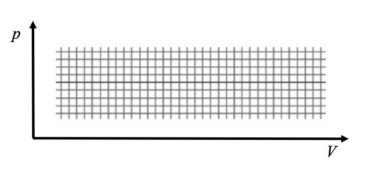
Figure 1: Possible discretization in $p$-$V$ space for use in testing different proposed temperature scales.

With the knowledge that fixing a single $T_{0}$ enables a meaningful temperature, the next section considers the more robust approach of satisfying (2) in a root-mean-square sense, as is almost universally done in matching theory and data.

From (2), with $T$ determined, it follows that, $dS=fdQ=dQ/T$ is a true differential, so that the entropy can be defined asClausius65

$$S=\int\frac{dQ}{T}+\hbox{const}.$$ (3)

The constant, of course, comes from the Third Law of Thermodynamics. Because $S$ depends only on other thermodynamic parameters, not on the history of the thermometer, $S$ is what is known as a thermodynamic state function.Sears ; Callen1 ; Fermi ; Reif

III Root-mean-square Deviation of Entropy

We now employ eq. (2) to develop a procedure to obtain $T(p,V)$ using the root-mean-square deviation from eq. (2) for each cell $i$.SaslowEJP20 In Fig. 1 the cell areas could be of any shape and area, but for simplicity we have taken them all to be rectangles with the same area.

Consider a given model temperature scale $T_{n}(p,V)$, where $n$ identifies the model (including functional form and any unknown parameters); for simplicity we hereafter suppress the dependence on $p$ and $V$. If there are $M$ such areas in the regions of interest, then the $i$-th area has a deviation

$$\Delta S_{i,n}=\oint_{i}\frac{dQ}{T_{n}}.$$ (4)

The sign of $\Delta S_{i,n}$ has no fundamental significance, and typically will be non-zero, either because the proposed $T_{n}$ is not the true thermodynamic temperature, or because of errors associated with the discretization, or errors in the measurement of the $dQ$’s. For each $i$, and a rectangular grid, four measurements of $dQ$ are required; a numerical approximation would take $T_{n}$ at the midpoint of each side.

The total rms (root-mean-square) deviation, summed over the grid of $M$ areas, is given by what we will call the net rms entropic “mismatch”

$$F_{n}=(\Delta S)^{2}_{{\rm tot},n}=\sum_{i=1}^{M}(\Delta S_{i,n})^{2}.$$ (5)

Of two temperature models $T_{n}$ and $T_{n^{\prime}}$, the preferred model is that with the smaller $(\Delta S)^{2}_{\rm tot}$; that is, the smaller net rms entropic “mismatch”.

As an example, let a temperature scale have a given functional form with three parameters, one of which can be thought of as determining $T_{0}(p_{0},V_{0})$. The best such temperature scale for this functional form is found by minimizing the rms value of (5) as a function of these three parameters for the region $\Omega$ of $(p,V)$ space. The approach may be generalized to different functional forms and numbers of parameters. Different regions can be stitched together to cover all of $p$-$V$ space.

Analogously, for a $T$-$S$ diagram – rather than a $p$-$V$ diagram – one could employ a net rms volumetric “mismatch” criterion. This would be based on the expectation that, with $dW$ the work done by the system, $\Delta V=\oint(dW/p)=0$ for each element of a thermodynamic $T$-$S$ grid. This can provide a check on values of thermodynamic quantities.

IV Statistical Mechanics Based Thermometries

Examples of thermometries based on statistical mechanics include:

(a) For a region that is accessible to an ideal, or nearly ideal, gas (with $n$ the number of moles and $R$ the gas constant), a proxy is

$$pV=nRT.$$ (6)

This equation works particularly well for dilute gases at somewhat elevated temperatures. Virial expansions give corrections to eq. (6).

(b) A thermometry for the cosmos uses the cosmic microwave background (CMB) radiation distribution. For frequency $\omega$ it satisfies the Bose-Einstein distribution

$$n(\omega)=[e^{(\hbar\omega/k_{B}T)}-1]^{-1}.$$ (7)

This thermometry also is employed in modern temperature “guns”.

(c) The magnetic susceptibility of a collection of nearly non-interacting nuclear spins at low temperatures (but not so low that interactions cause the nuclear spins to order) satisfies

$$\chi=\frac{C}{T},$$ (8)

where $C$ is the Curie constant. This is the ideal gas of magnetism.

(d) Noise thermometry, where the noise power $P_{W}$ (watts) over a bandwidth $B$ (hertz) satisfies

$$\frac{P_{W}}{B}=k_{B}T,$$ (9)

where $k_{B}$ is the Boltzmann constant. Noise thermometry is often employed at low temperatures.

The author was introduced to the issue of thermometry at an International Conference on Low Temperature Physics. There two distinguished, prize-winning, low temperature physicists, who each used both susceptibility and noise thermometries, disputed which was better.SaslowEJP20 For specific examples of practical thermometry, see Refs. Moldover, ; Tuoriniemi, ; Mazon, ; Casey, ; Saunders, . Also note Ref. TempReview19, .

V Beyond Statistical Mechanics: New Types of Thermometers

In the absence of a thermometer or a material with properties simple enough to be described by a statistical mechanical theory, a lab must develop its own thermometer. Although we earlier indicated that almost any material would serve, in practice some materials could give problems. For example, if the material is a combination of two substances, such as air and water, then condensation or evaporation of the water might complicate the analysis.

A possible thermometer material is an interacting gas that is too dense to be described by a statistical mechanical virial expansion. However, it has the advantage that accurate pressure and volume measurements should be relatively simple to perform. In the same spirit is an interacting set of spins, where accurate magnetic field, volume, and pressure measurements should be relatively simple to perform.

In the Clausius based approach a lab can calibrate two nominally identical materials without concern that they are not identical. In principle they would both yield the same – or nearly the same – temperature scale, although the $dQ$’s would differ, as would the derived entropies $S$.

VI Refining Measurements of Heat

In practice, fundamental thermometry currently is performed by measuring an appropriate system, and analyzing it using a statistical mechanical theory. If the resulting temperature $T$ is more accurate than a corresponding Clausius based based temperature scale from an rms minimization of (5) then, as is often done with standards, one can turn the problem around, and correct the heat input measurements.

For measured heat inputs $dQ_{m}$, one uses the proxy temperature and assumes a dimensionless correction factor $F(T)$ with a few unknown parameters to obtain

$$G=\sum_{i}\int_{i}\Big{(}\frac{dQ_{m}F(T)}{T}\Big{)}^{2}.$$ (10)

Once $F(T)$ is determined by the minimization process, the corrected heat input $dQ_{c}$ is given by

$$dQ_{c}=dQ_{m}F(T).$$ (11)

In this way, the standards for measurement of heat input $dQ$ can be raised to the level of accuracy of the proxy-based temperature scale. Ref. SaslowF=ma, indicates how a standard can be improved by the use of a physical law.

It is unfortunate that there is no thermodynamic unit named after Clausius, who gave us the first correct thermodynamics,ClausiusThermo ; GibbsHistoryThermo and both introducedClausius54 and first understood entropy.Clausius65 ; GibbsHistoryThermo A unit for entropy would surely be the clausius (Cl), rather than the (derived) joule/kelvin (J/K). It is perhaps not coincidental that there was a priority dispute between Clausius and Kelvin.SaslowBriefHistory

VII Summary

We have, more explicitly than previously, indicated how thermometry can be performed using a Clausius-based approach. We observed that there are three types of thermometry, and that only the Clausius-based version is based solely on thermodynamics. Thus it is suitable to employ nearly any material as a thermometer, not merely those for which there are statistical mechanical theories.

VIII Acknowledgements

I would like to acknowledge valuable interactions with C. Meyer and N. Mirabolfathi.

References

- (1) F. W. Sears, An Introduction to Thermodynamics, The Kinetic Theory of Gases, and Statistical Mechanics, Second edition, Addison-Wesley, Reading, MA, 1953. This work is very closely coupled to experiment, including a discussion of steam engines, whose efficiency motivated Carnot’s work.
- (2) H. B. Callen, Thermodynamics, Wiley, New York, 1961.
- (3) E. Fermi, Thermodynamics, Dover, 1956. Based on 1937 lecture notes.
- (4) F. Reif, Fundamentals of Statistical and Thermal Physics, McGraw-Hill, 1967.
- (5) R. Clausius, Annalen der Physik und der Chemie, Vol. 125 (1865), pp. 353-400. Translated in “On the Determination of the Energy and Entropy of a Body,” Phil. Mag. S4, Vol. 32, pp. 1-17 (1866).
- (6) Before he recognized the physical significance of entropy, Clauisius had already derived this relation, using for . R. Clausius, Poggendoff’s Annalen, December 1854, vol. xciii. p. 481; translated in the Journal de Mathematiques, Vol. XX. Paris, 1855, and in the Philosophical Magazine, August 1856, S4. Vol. 22, p. 81 (1856). This was available online at wikisource.
- (7) For a basic Carnot cycle involving two temperatures one has . Even if one does not know the values of and , by use of a proxy thermometer it may be possible to ensure that and are fixed. If one then fixes, say, at a triple point value, then measuring and will then give . This approach can be performed, but having to always ensure that the proxy thermometer is fixed may be a complicating issue in a practical sense. On the other hand it shows that once the temperature is fixed at one point in space, it is then determined at all other points in ( space. For small changes in or one must verify that and are constant to second order in these small changes. The integral approach we describe does not have that issue.
- (8) W. M. Saslow, Eur. J. Phys. 41, 055101 (2020), 11 pages. “Entropy Uniqueness Determines Temperature”.
- (9) M. R. Moldover, Weston L. Tew and H. W. Yoon, Nature Physics, 12, 7 (2016). “Advances in thermometry.” The article notes that details may be found in J. Fischer, M. de Podesta, K. D. Hill, M. Moldover, L. Pitre, R. Rusby, P. Steur, O. Tamura, R. White and L. Wolber, Int. J. Thermophys. 32, 12 (2011) “Present Estimates of the Differences Between Thermodynamic Temperatures and the ITS-90” and J. Fischer, Metrologia 52, S364 (2015) “Progress toward a new definition of the kelvin.”
- (10) J. Tuoriniemi, Nature Physics, 12, 11 (2016). “Physics at its coolest.”
- (11) D. Mazon, C. Fenzi and R. Sabot, Nature Physics, 12, 14 (2016). “As Hot as it Gets.”
- (12) A. Casey, F. Arnold, L. V. Levitin, C. P. Lusher, J. Nyéki, J. Saunders, A. Shibahara, H. van der Vliet, B. Yager, D. Drung, Th. Schurig, G. Batey, M. N. Cuthbert, A. J. Matthews, J. Low Temp. Phys. 175, 764-775 (2014). “Current Sensing Noise Thermometry: A Fast Practical Solution to Low Temperature Measurement.”
- (13) A. Shibahara, O. Hahtela, J. Engert, H. van der Vliet, L. V. Levitin, A. Casey, C. P. Lusher, J. Saunders, D. Drung and Th. Schurig, Roy Soc. Phil. Trans. A, 374, 20150054 (2016). “Primary current-sensing noise thermometry in the millikelvin regime.”
- (14) M. Mehboudi, A. Sanpera, and L. A. Correa, J. Phys. A: Math. Theor. 52, 303001 (2019) 49 pages. “Thermometry in the quantum regime: recent theoretical progress”.
- (15) W. M. Saslow, Am. J. Phys. 82, 349-353 (2014). “Accurate physical laws can permit new standard units: The two laws and the proportionality of weight to mass.”
- (16) R. Clausius, Poggendorf’s Annelen, Vol. 79, p. 368 (1850). English translation in Phil. Mag. S4, Vol. 2, p.1 (1851). “On the Moving Force of Heat, and the Laws regarding the Nature of Heat itself which are deducible therefrom.”
- (17) J. W. Gibbs, “Rudolf Julius Emanuel Clausius,” Proc. Amer. Acad. 16 (1889), 458. Reprinted in The Scientific Papers of J. Willard Gibbs (New York, 1906; reprinted 1961), Vol. 2, 261-267.
- (18) W. M. Saslow, Entropy 22, 77 (2020), 48 pages. “A History of Thermodynamics: the Missing Manual.” doi:10.3390/e22010077.