ERA-Solver: Error-Robust Adams Solver
for Fast Sampling of Diffusion Probabilistic Models

Abstract

Though denoising diffusion probabilistic models (DDPMs) have achieved remarkable generation results, the low sampling efficiency of DDPMs still limits further applications. Since DDPMs can be formulated as diffusion ordinary differential equations (ODEs), various fast sampling methods can be derived from solving diffusion ODEs. However, we notice that previous sampling methods with fixed analytical form are not robust with the error in the noise estimated from pretrained diffusion models. In this work, we construct an error-robust Adams solver (ERA-Solver), which utilizes the implicit Adams numerical method that consists of a predictor and a corrector. Different from the traditional predictor based on explicit Adams methods, we leverage a Lagrange interpolation function as the predictor, which is further enhanced with an error-robust strategy to adaptively select the Lagrange bases with lower error in the estimated noise. Experiments on Cifar10, LSUN-Church, and LSUN-Bedroom datasets demonstrate that our proposed ERA-Solver achieves 5.14, 9.42, and 9.69 Fenchel Inception Distance (FID) for image generation, with only 10 network evaluations.

1 Introduction

In recent years, denoising diffusion probabilistic models (DDPMs) (Ho et al., 2020) have been proven to have potential in data generation tasks such as text-to-image generation(Poole et al., 2022; Gu et al., 2022; Kim & Ye, 2021; Chen et al., 2022), speech synthesis(Huang et al., 2021; Lam et al., 2022; Leng et al., 2022), and molecular conformation formation(Hoogeboom et al., 2022; Jing et al., 2022; Wu et al., 2022; Huang et al., 2022). They build a diffusion process to add noise into the sample and a denoising process to remove noise from the sample gradually. Compared with generative adversarial networks (GANs)(Goodfellow et al., 2014) and variational auto-encoders (VAEs)(Child, 2021), DDPMs have achieved remarkable generation quality. However, due to the properties of the Markov chain, the sampling process requires hundreds or even thousands of denoising steps. Such defects limit the wide applications of diffusion models. Thus, it is an urgent request for a fast sampling of DDPMs.

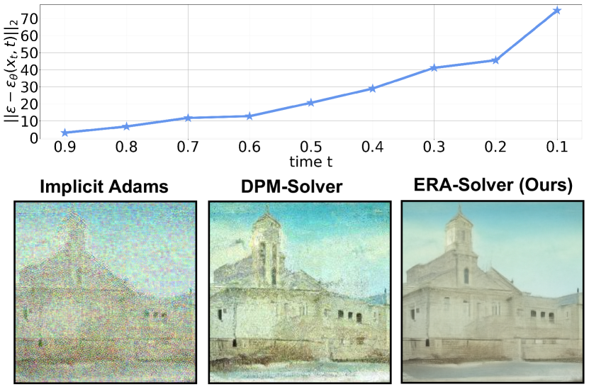
Figure 1: We adopt the pretrained diffusion model from (Song et al., 2020a) and visualize the error between the estimated noise and ground-truth noise in training. We also provide the generated samples from the pretrained model based on implicit Adams (traditional predictor-corrector method (Diethelm et al., 2002)), DPM-Solver(Lu et al., 2022a), and our error-robust Adams solver (ERA-Solver). Our solver is robust for the error from pretrained model so as to generate samples with better quality.

There have already existed many works for accelerating sampling speed. Some works introduced an extra training stage, such as knowledge distillation method (Salimans & Ho, 2021), training sampler (Watson et al., 2021), or directly combining with GANs (Wang et al., 2022), to obtain a fast sampler. These methods require a cumbersome training process for each task, and are black-box samplers due to the lack of theoretical explanations. Denoising diffusion implicit model (DDIM) (Song et al., 2020a) and Score-SDE(Song et al., 2020b) revealed that the sampling can be reformulated as a diffusion ordinary differential equation (ODE) solving process, which inspired many works to design learning-free fast samplers based on numerical methods. PNDM (Liu et al., 2021) introduced the analytic form of a 4-order linear multistep method, which is also called explicit Adams method (Małgorzata & Marciniak, 2002), and utilized the estimated noises observed at previous sampling steps to sample efficiently, with a warming initialization based on Runge-Kutta methods (Butcher, 1996). DPM-Solver(Lu et al., 2022a) introduced exponential integrator from ODE literature (Atkinson et al., 2011) and required extra network evaluations to observe intermediate noise terms for approximating Taylor expansion (Mohazzabi & Becker, 2017) in the sampling process.

The existing learning-free methods (Liu et al., 2021; Lu et al., 2022a; Song et al., 2020a) are based on the assumption that the learned network has high accuracy in noise estimations across all the sampling steps. However, we notice that the noise estimated from the neural network is not accurate enough and the error exists at almost every time $t$, especially when time $t$ approaches $0$, as shown in Fig. 1. Existing sampling methods are not able to be robust for noise estimation errors, since they consist of an analytic sampling scheme with fixed coefficients to ensure sampling convergence. For example, explicit Adams (Małgorzata & Marciniak, 2002) consists of the analytic form with fixed coefficients as formulated in Eq. 9.

In this paper, we aim at designing an error-robust diffusion ODE solver to speed up the sampling process of DDPMs while achieving good sampling quality. To this end, we focus on implicit Adams solver (Małgorzata & Marciniak, 2006), a kind of numerical ODE solver, which involves unobserved terms to achieve high-order precision and convergence. In existing ODE literature(Atkinson et al., 2011), predictor-corrector has been introduced to perform implicit Adams solver, which avoids solving the implicit equation. Explicit Adams usually acts as the predictor to predict the unobserved term. However, traditional predictor-corrector still suffers from the inaccurate estimation of diffusion noise at each sampling step since it is composed of fixed coefficients, which is shown in Fig. 1. Instead of utilizing explicit Adams as the predictor, we adopt the Lagrange interpolation function (Sauer & Xu, 1995) that interpolates several Lagrange function bases as the predictor. We maintain a buffer of estimated noises observed at previous sampling steps during sampling and adaptively select those estimated noises with low estimation error as the Lagrange function bases, to ensure accurate interpolation result and thus an accurate predictor. In this way, we can obtain a diffusion ODE sampler with not only high convergence (thanks to the implicit Adams method(Małgorzata & Marciniak, 2006)) but also good error robustness (thanks to the adaptive strategy for the Lagrange interpolation function).

However, it is not easy to select noises with low estimation error as the Lagrange function bases. That is because, unlike the training stage, there exist no reference noises at the sampling stage to judge how accurate the estimated noise is. Thus, we further propose an approach to roughly measure the accuracy of the estimated noise by calculating the difference between the noise obtained by the predictor (as the prediction) and the noise observed at the previous sampling step (as the reference). Based on this measurement, we propose a selection strategy for the buffer which adaptively chooses estimated noises that are more accurate to construct the Lagrange function bases, so as to result in a more accurate predictor, and thus a better ODE solver.

Our contributions can be summarized as follows:

• We are the first to explore the potential of numerical implicit Adams methods (Małgorzata & Marciniak, 2006) to solve diffusion ODEs. We propose an error-robust implicit Adams Solver (ERA-Solver), which is training-free and can be extended to pretrained DDPMs conveniently.

• We propose to adopt the Lagrange interpolation function (Sauer & Xu, 1995) that selectively interpolates several Lagrange function bases with low errors of estimated noises to ensure the ERA-solver is robust to the error in estimated noise.

• Experiment results show that we achieve better results on LSUN-Bedroom, LSUN-Church, and Cifar10 datasets when compared with previous methods in 10 function evaluations. On LSUN-Church and LSUN-Bedroom, we achieve state-of-the-art FID results of 7.39 and 5.39 with more function evaluations, compared with the previous best results of 7.74 and 6.46.

2 Preliminary

2.1 Denoising Diffusion Probabilistic Models

Denoising diffusion probabilistic models (DDPMs)(Ho et al., 2020) have demonstrated their great generation potential on various applications, such as text-to-image synthesis (Poole et al., 2022; Gu et al., 2022; Kim & Ye, 2021), image inpainting (Lugmayr et al., 2022; Liu et al., 2022; Kawar et al., 2022), speech synthesis (Huang et al., 2021; Lam et al., 2022; Leng et al., 2022), and molecular conformation generation (Hoogeboom et al., 2022; Jing et al., 2022; Wu et al., 2022; Huang et al., 2022). It involves a diffusion process to gradually add noise to data, and a parameterized denoising process to reverse the diffusion process, sampling through gradually removing the noise from random noise. The diffusion process is modeled as a transition distribution:

$$q(\mathbf{x}_{t}|\mathbf{x}_{t-1}):=\mathcal{N}(\mathbf{x}_{t};\sqrt{\alpha_{t}}\mathbf{x}_{t-1},(1-\alpha_{t})\mathbf{I}),$$ (1)

where $\alpha_{1},...,\alpha_{T}$ are fixed parameters. With the transition distribution above, noisy distribution conditioned on clean data $x_{0}$ can be formulated as follows:

$$q(\mathbf{x}_{t}|\mathbf{x}_{0})=\mathcal{N}(\mathbf{x}_{t};\sqrt{\overline{\alpha}_{t}}\mathbf{x}_{0},(1-\overline{\alpha}_{t})\mathbf{I}),$$ (2)

where $\bar{\alpha}_{t}=\prod_{s=1}^{t}\alpha_{s}$. When $t$ is large enough, the Markov process will converge to a Gaussian steady-state distribution $\mathcal{N}(0,I)$.

DDPMs also build the reverse process, i.e., the sampling process, to the diffusion process above. Similar to VAEs, DDPMs introduce the variational bound to derive optimization objectives. After simplification (Luo, 2022), the main objective of training optimization is formulated as a KL divergence:

$$\begin{split}L_{t-1}=\mathcal{D}_{KL}(q(\mathbf{x}_{t-1}|\mathbf{x}_{0},\mathbf{x}_{t})||p_{\theta}(\mathbf{x}_{t-1}|\mathbf{x}_{t})),\end{split}$$ (3)

where $q(\mathbf{x}_{t-1}|\mathbf{x}_{0},\mathbf{x}_{t})$ has an analytical form derived from the bayesian formula and can be expressed as a Gaussian distribution parameterized with $\mu_{t-1}=\frac{1}{\sqrt{\alpha_{t}}}(\mathbf{x}_{t}-\frac{1-\alpha_{t}}{\sqrt{1-\bar{\alpha}_{t}}}{\boldsymbol{\epsilon}})$ and $\sigma_{t-1}=\frac{1-\bar{\alpha}_{t-1}}{1-\bar{\alpha}_{t}}(1-\alpha_{t})$.

To simplify the optimization loss, the parameterized denoising distribution is formulated as follows:

$$\begin{split}p_{\theta}(\mathbf{x}_{t-1}|\mathbf{x}_{t})=\mathcal{N}(\mathbf{x}_{t-1};\mu_{\theta}(\mathbf{x}_{t}),{\sigma}_{t-1}^{2}\mathbf{I})\\ \mu_{\theta}(\mathbf{x}_{t})=\frac{1}{\sqrt{\alpha_{t}}}(\mathbf{x}_{t}-\frac{1-\alpha_{t}}{\sqrt{1-\bar{\alpha}_{t}}}{\boldsymbol{\epsilon}}_{\theta}(\mathbf{x}_{t},t)),\end{split}$$ (4)

where ${\boldsymbol{\epsilon}}_{\theta}(\mathbf{x}_{t},t)$ estimates the noise in noisy sample $\mathbf{x}_{t}$ and is called estimated noise in our paper. The variance $\sigma_{t-1}^{2}$ is constant. In this way, the objective function Eq. 3 can be rewritten as following:

$$\small\begin{split}L_{t-1}&=\mathbb{E}_{q}[\frac{1}{2\sigma_{t-1}^{2}}||\mu_{t-1}-\mu_{\theta}(\mathbf{x}_{t})||^{2}]\\ &=\mathbb{E}_{x_{0},{\boldsymbol{\epsilon}}}[\frac{1}{2\sigma_{t-1}^{2}}||\frac{1}{\sqrt{\alpha_{t}}}(\mathbf{x}_{t}-\frac{1-\alpha_{t}}{\sqrt{1-\bar{\alpha}_{t}}}{\boldsymbol{\epsilon}})-\mu_{\theta}(\mathbf{x}_{t})||^{2}]\\ &=\mathbb{E}_{\mathbf{x}_{0},{\boldsymbol{\epsilon}}}[\frac{1}{2\sigma_{t-1}^{2}}\frac{(1-\alpha_{t})^{2}}{\alpha_{t}(1-\bar{\alpha}_{t})}||{\boldsymbol{\epsilon}}-{\boldsymbol{\epsilon}}_{\theta}(\mathbf{x}_{t},t)||^{2}].\end{split}$$ (5)

Though DDPMs have good theoretical properties, they suffer from sampling efficiency. It usually requires hundreds or even thousands of network evaluations, which limits various downstream applications for DDPMs. There already existed methods (Watson et al., 2021; Lyu et al., 2022; Lam et al., 2022; Salimans & Ho, 2021) which depend on extra training stage to derive fast sampling methods. The training-based methods usually require tremendous training costs for different data manifolds and tasks, which inspires many works to explore a training-free sampler based on numerical methods.

2.2 Numerical Methods for Fast Sampling

Denoising diffusion implicit model (DDIM) (Song et al., 2020a) is a classic training-free approach for fast sampling, which introduces a non-Markovian process that allows the sampling with any number of evaluation steps. We formulate the iteration time steps for solving diffusion ODEs as $\{t_{i}\}_{i=0}^{N}$, where $t_{0}$ is the beginning time and $t_{N}$ is the end time. The sequence of sampling steps maintains the property that $t_{i}\textgreater t_{i+1}$ and $t_{N}=0$. In particular, the last iterate $x_{t_{N}}$ represents the final generated sample. The denoising iteration process of DDIM can be formulated as follows:

$$\begin{split}\mathbf{x}_{t_{i+1}}=\sqrt{\bar{\alpha}_{t_{i+1}}}(\frac{\mathbf{x}_{t}-\sqrt{1-\bar{\alpha}_{t_{i}}}{\boldsymbol{\epsilon}}_{\theta}(\mathbf{x}_{t_{i}},t_{i})}{\sqrt{\bar{\alpha}_{t_{i}}})}\\ +\sqrt{1-\bar{\alpha}_{t_{i+1}}-\sigma_{t_{i}}^{2}}{\boldsymbol{\epsilon}}_{\theta}(\mathbf{x}_{t_{i}},t_{i})+\sigma_{t_{i}}\mathbf{\mathbf{z}}.\end{split}$$ (6)

Furthermore, DDIM shares the same training objective with DDPMs, which means the fast sampling scheme can be applied to any pre-trained models. When the variance $\sigma_{t_{i}}^{2}$ is set to 0, the sampling process becomes deterministic, which can be regarded as the solving process of diffusion ODEs. We use a term ${\boldsymbol{\epsilon}}_{t_{i}}$ for the ease of description so that the solving formula of diffusion ODE can be formulated (Song et al., 2020a) as follows:

$$\small{\boldsymbol{\epsilon}}_{t_{i}} ={\boldsymbol{\epsilon}}_{\theta}(x_{t_{i}},t_{i}),$$ (7)

$$\mathbf{x}_{t_{i+1}} =\frac{\sqrt{\bar{\alpha}_{t_{i+1}}}}{\sqrt{\bar{\alpha}_{t_{i}}}}x_{t_{i}}$$

$$+(\sqrt{1-\bar{\alpha}_{t_{i+1}}}-\frac{\sqrt{\bar{\alpha}_{t_{i+1}}(1-\bar{\alpha}_{t_{i}})}}{\sqrt{\bar{\alpha}_{t_{i}}}}){\boldsymbol{\epsilon}}_{t_{i}}.$$ (8)

Many numerical solvers, such as Runge-Kutta (Butcher, 1996) method and linear multistep method (Wells, 1982), can be applied to solve diffusion ODEs. PNDM(Liu et al., 2021) combined Runge-Kutta and linear multistep method so as to solve the manifold problem of diffusion ODEs. Essentially, the linear multistep method can be regarded as explicit Adams (Małgorzata & Marciniak, 2002), which utilized previously estimated noises to calculate the ${\boldsymbol{\epsilon}}_{t_{i}}$. The ${\boldsymbol{\epsilon}}_{t_{i}}$ in Eq. 7 is reformulated as following:

$${\boldsymbol{\epsilon}}_{t_{i}} =\frac{1}{24}(55{\boldsymbol{\epsilon}}_{\theta}(\mathbf{x}_{t_{i}},t_{i})-59{\boldsymbol{\epsilon}}_{\theta}(\mathbf{x}_{t_{i-1}},t_{i-1})$$ (9)

$$+37{\boldsymbol{\epsilon}}_{\theta}(\mathbf{x}_{t_{i-2}},t_{i-2})-9{\boldsymbol{\epsilon}}_{\theta}(\mathbf{x}_{t_{i-3}},t_{i-3})).$$

DPM-Solver(Lu et al., 2022a) introduced the method of exponential integrator from ODE literature (Atkinson et al., 2011) to eliminate the discretization errors of the linear term in the sampling process. Furthermore, DPM-Solver proposed to utilize Taylor expansion (Mohazzabi & Becker, 2017) to approximate ${\boldsymbol{\epsilon}}_{t_{i}}$ and contributed its analytical forms for solving diffusion ODEs.

We notice that the estimated noises of pretrained diffusion models are not precise across all sampling time, especially when time $t_{i}$ is close to $0$. Previous numerical methods with analytical forms will suffer from the noise estimation error of pretrained DDPMs. In this paper, we propose an error-robust solver based on Adams numerical methods, adaptively selecting noises with low estimation error.

3 ERA-Solver

In this section, we first point out that the error in the estimated noise ${\boldsymbol{\epsilon}}_{\theta}(\mathbf{x}_{t_{i}},t_{i})$ by the network $\theta$ limits the previous numerical fast samplers and introduce implicit Adams numerical solver (Sec. 3.1). Then, we apply predictor-corrector sampling and leverage a Lagrange interpolation function as the predictor (Sec. 3.2). We design an error distance to measure the accuracy of the estimated noise and enhance the proposed predictor with an error-robust strategy to adaptively select the Lagrange bases with lower noise estimation error (Sec. 3.3). The whole sampling process is shown in Fig. 2.

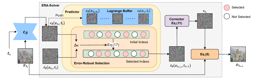
Figure 2: The pipeline of ERA-Solver. The sampling scheme is based on the predictor-corrector method for implicit Adams. Our predictor is robust to the errors of the estimated noises from pretrained models. The sampling starts from normal Gaussian noise $x_{t_{0}}$ and performs a denoising scheme (from $x_{t_{i}}$ to $x_{t_{i+1}}$) iteratively to get the final generated image.

3.1 Implicit Adams Methods

The sampling of DDPMs starts from a prior noise distribution $\mathbf{x}_{t_{0}}\sim\mathcal{N}(0,I)$, and iteratively denoises $\mathbf{x}_{t_{i}}$ to $\mathbf{x}_{t_{i+1}}$ until time $t$ reaches $0$. In the sampling process, the most time-consuming step is network evaluation. Assuming we have a pretrained noise estimation model ${\boldsymbol{\epsilon}}_{\theta}$, we need to achieve good generation quality with as few evaluation times as possible.

We notice that the noise estimation error exists across every sampling time, especially when time $t_{i}$ is close to 0. It limits previous numerical high-order solvers (Liu et al., 2021; Lu et al., 2022a; Song et al., 2020a) since they are based on the assumption that the network has no estimation errors. Previous solvers usually involved observed noise terms to achieve the analytic form of the sampling scheme that is critical for sampling convergence. Thus, they are sensitive to the errors of estimated noises from pretrained models.

In this paper, we explore the potential of implicit Adams solver (Małgorzata & Marciniak, 2006). Different from explicit Adams (Eq. 9), implicit Adams involves the unobserved noise term and the ${\boldsymbol{\epsilon}}_{t_{i}}$ in Eq. 7 is reformulated as follows:

$${\boldsymbol{\epsilon}}_{t_{i}} =\frac{1}{24}(9{\boldsymbol{\epsilon}}_{\theta}(\mathbf{x}_{t_{i+1}},t_{i+1})+19{\boldsymbol{\epsilon}}_{\theta}(\mathbf{x}_{t_{i}},t_{i})$$ (10)

$$-5{\boldsymbol{\epsilon}}_{\theta}(\mathbf{x}_{t_{i-1}},t_{i-1})+{\boldsymbol{\epsilon}}_{\theta}(\mathbf{x}_{t_{i-2}},t_{i-2})).$$

It can be noticed that $\mathbf{x}_{t_{i+1}}$ can be observed only when ${\boldsymbol{\epsilon}}_{t_{i}}$ is achieved, while the ${\boldsymbol{\epsilon}}_{t_{i}}$ contains unobserved term ${\boldsymbol{\epsilon}}_{\theta}(\mathbf{x}_{t_{i+1}},t_{i+1})$, which makes it challenging to solve implicit equations and may need more time-consuming iteration steps. This greatly limits the implicit Adams method to be a fast solver for diffusion ODEs.

Fortunately, in numerical ODE literature, the sampling efficiency of implicit Adams can be improved with a predictor-corrector sampling scheme (Diethelm et al., 2002). Specifically, the predictor makes a rough estimation of unobserved term $\bar{\boldsymbol{\epsilon}}_{\theta}(\mathbf{x}_{t_{i+1}},t_{i+1})$ and the corrector derives the precise $\mathbf{x}_{t_{i+1}}$, which can reformulate Eq.10 as follows:

$${\boldsymbol{\epsilon}}_{t_{i}} =\frac{1}{24}(9\bar{\boldsymbol{\epsilon}}_{\theta}(\mathbf{x}_{t_{i+1}},t_{i+1})+19{\boldsymbol{\epsilon}}_{\theta}(\mathbf{x}_{t_{i}},t_{i})$$ (11)

$$-5{\boldsymbol{\epsilon}}_{\theta}(\mathbf{x}_{t_{i-1}},t_{i-1})+{\boldsymbol{\epsilon}}_{\theta}(\mathbf{x}_{t_{i-2}},t_{i-2})).$$

The traditional predictor-corrector utilizes explicit Adams (Eq. 9) to perform predictor to make $\mathbf{x}_{t_{i+1}}$ observed so as to derive $\bar{\boldsymbol{\epsilon}}_{\theta}(\mathbf{x}_{t_{i+1}},t_{i+1})$. However, it still suffers from the fixed form that is not robust to the noise estimation errors, which can be observed in Fig. 1.

3.2 Predictor with Lagrange Interpolation Function

In this paper, we propose to utilize noises observed at previous sampling steps and construct the Lagrange interpolation function as the predictor to predict unobserved term ${\boldsymbol{\epsilon}}_{\theta}(\mathbf{x}_{t_{i+1}},t_{i+1})$. In this way, we can design an adaptive strategy to select Lagrange function bases to construct the error-robust predictor.

Specifically, we maintain a buffer about all previously estimated noises, which have been observed and need no extra computations, and its corresponding time:

$$\{(t_{n},{\boldsymbol{\epsilon}}_{\theta}(\mathbf{x}_{t_{n}},t_{n})),n=0,1,..,i\}.$$ (12)

The maintained buffer is also called the Lagrange buffer in this paper. Assume that the interpolation order is $k$, the selected function bases to construct the Lagrange function can be written as $\{(t_{\tau_{m}},{\boldsymbol{\epsilon}}_{\theta}(\mathbf{x}_{t_{\tau_{m}}},t_{\tau_{m}})),m=0,...k-1\}$. The corresponding Lagrange interpolation function can be formulated as:

$$l_{m}(t) =\prod_{l=0,l\neq m}^{k-1}(\frac{t-t_{\tau_{l}}}{t_{\tau_{m}}-t_{\tau_{l}}}),$$ (13)

$$L_{{\boldsymbol{\epsilon}}}(t) =\sum_{m=0}^{k-1}l_{m}(t)*{\boldsymbol{\epsilon}}_{\theta}(\mathbf{x}_{t_{\tau_{m}}},t_{\tau_{m}}),$$

where $\tau_{l}$ belongs to the maintained Lagrange buffer and has already been observed. At time $t_{i+1}$, we can derive an estimation about ${\boldsymbol{\epsilon}}_{\theta}(\mathbf{x}_{t_{i+1}},t_{i+1})$:

$$\bar{\boldsymbol{\epsilon}}_{\theta}(\mathbf{x}_{t_{i+1}},t_{i+1})=L_{{\boldsymbol{\epsilon}}}(t_{i+1}).$$ (14)

With this prediction, we apply the corrector process in Eq. 11 to get the ${\boldsymbol{\epsilon}}_{t_{i}}$ and Eq. 8 to get the denoised sample $\mathbf{x}_{t_{i+1}}$.

It can be noticed that the proposed predictor makes use of the observed noise estimations and involves no network evaluations. Furthermore, the Lagrange bases in the predictor can be adaptively selected from those noise estimations with low errors, which is more error-robust. We introduce this error-robust selection strategy in the next subsection.

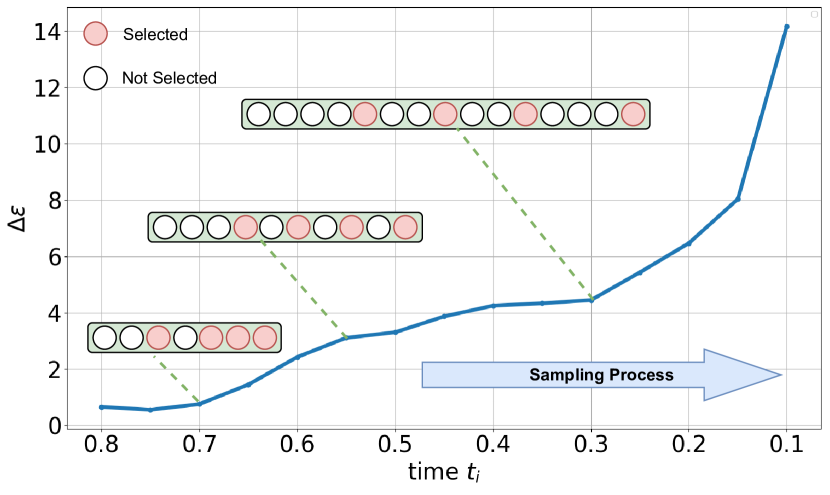
Figure 3: Error-robust selection process. $\Delta\epsilon$ is calculated based on Eq. 15 instead of the training loss in Fig. 1. The sampling NFE is set to 20.

3.3 Error-Robust Selection Strategy

In this part, our goal is to design an error-robust selection strategy for the maintained Lagrange buffer. When the interpolation order is $k$, the intuitive selection approach is to make a fixed selection of the last $k$ estimated noises from the maintained Lagrange buffer, which means $\tau_{m}=i-m$ in Eq. 13. However, we notice that the noise estimation error tends to increase as time $t_{i}$ approaches $0$ (Fig. 1), in which case the fixed selection strategy may aggregate the noise estimation errors from Lagrange buffer and make the constructed Lagrange function inaccurate for prediction at time $t_{i+1}$. It motivates us to seek a reasonable measure of the error in estimated noise so as to select those noises with low estimation error for Lagrange interpolation.

Error Measure for Estimated Noise.

Since there exists no ground-truth noise in sampling process, it is hard to measure the error in estimated noise. To this end, we propose to utilize the observed noise term ${\boldsymbol{\epsilon}}_{\theta}(\mathbf{x}_{t_{i}},t_{i})$ as the target noise and the predicted noise term $\bar{\boldsymbol{\epsilon}}_{\theta}(\mathbf{x}_{t_{i}},t_{i})$ from last sampling step as the estimated noise to calculate the approximation error, which can be seen in Fig. 2. It can be formulated as follows:

$$\Delta{\boldsymbol{\epsilon}}=||{\boldsymbol{\epsilon}}_{\theta}(\mathbf{x}_{t_{i}},t_{i})-\bar{\boldsymbol{\epsilon}}_{\theta}(\mathbf{x}_{t_{i}},t_{i})||_{2}.$$ (15)

${\boldsymbol{\epsilon}}_{\theta}(\mathbf{x}_{t_{i}},t_{i})$ is observed based on $x_{t_{i}}$, which is achieved via the $\bar{\boldsymbol{\epsilon}}_{\theta}(\mathbf{x}_{t_{i}},t_{i})$ and Eq. 8. When the error of estimated noise from pretrained models increases, it tends to be hard for $\bar{\boldsymbol{\epsilon}}_{\theta}(\mathbf{x}_{t_{i}},t_{i})$ to approximate ${\boldsymbol{\epsilon}}_{\theta}(\mathbf{x}_{t_{i}},t_{i})$. As shown in Fig.3, our error measure in the sampling process shares the same trend as the error of estimated noises in the training process (Fig. 1), which demonstrates the rationality of the proposed error measure.

Algorithm 1 ERA-Solver

1:  Input: $\{t_{i}\}_{i=0}^{N},k,{\boldsymbol{\epsilon}}_{\theta}$

2:  Instantiate: ${\mathbf{x}}_{t_{0}}\sim\mathcal{N}(0,\mathbf{I})$, buffer $\Omega=\varnothing$, $\Delta{\boldsymbol{\epsilon}}=\lambda$

3:  $\Omega=\Omega\cup\{(t_{0},{\boldsymbol{\epsilon}}_{\theta}(\mathbf{x}_{t_{0}},t_{0}))\}$

4:  for $i$ in $0,1,\cdots,N-1$ do

5:     if $i\textless k-1$ then

6:        Derive $x_{t_{i+1}}$ based on Eq. 8 and ${\boldsymbol{\epsilon}}_{\theta}(\mathbf{x}_{t_{i}},t_{i})$

7:        $\Omega=\Omega\cup\{(t_{i+1},{\boldsymbol{\epsilon}}_{\theta}(\mathbf{x}_{t_{i+1}},t_{i+1}))\}$

8:     else

9:        Calculate $\{\bar{\tau}_{m}\}_{m=0}^{k-1}$ via Eq. 16

10:        Calculate $\{\tau_{m}\}_{m=0}^{k-1}$ via Eq. 17 and $\Delta{\boldsymbol{\epsilon}}$

11:        Derive Lagrange function $L_{{\boldsymbol{\epsilon}}}$ via Eq. 13 and $\tau_{m}$

12:        $\bar{\boldsymbol{\epsilon}}_{\theta}(\mathbf{x}_{t_{i+1}},t_{i+1})\leftarrow L_{{\boldsymbol{\epsilon}}}(t_{i+1})$

13:        Calculate ${\boldsymbol{\epsilon}}_{t_{i}}$ via $\Omega$, $\bar{\boldsymbol{\epsilon}}_{\theta}(\mathbf{x}_{t_{i+1}},t_{i+1})$, and Eq. 11

14:        Derive $\mathbf{x}_{t_{i+1}}$ based on Eq. 8 and ${\boldsymbol{\epsilon}}_{t_{i}}$

15:        $\Omega=\Omega\cup\{(t_{i+1},{\boldsymbol{\epsilon}}_{\theta}(\mathbf{x}_{t_{i+1}},t_{i+1}))\}$

16:        Update $\Delta{\boldsymbol{\epsilon}}$ via Eq. 15 and $\bar{\boldsymbol{\epsilon}}_{\theta}(\mathbf{x}_{t_{i+1}},t_{i+1})$

17:     end if

18:  end for

19:  return $\mathbf{x}_{t_{N}}$

Selection Strategy.

The high-level idea of our error-robust selection strategy is that we tend to choose those estimated noises from Lagrange buffer with low errors measured by Eq. 15 as the Lagrange bases. When sampling at time $t_{i}$, the length of the Lagrange buffer is $i+1$. We initialize $k$ indexes uniformly to cover the whole buffer:

$$\widehat{\tau}_{m}=(i/k)*m,m=1,2,..,k$$ (16)

Then we utilize the power function as an index translator. We parameterize the power function with the error measure (Eq. 15) so that the translation of initial indexes can be formulated as:

$$\tau_{m}=\lfloor(\widehat{\tau}_{m}/i)^{{\Delta{\boldsymbol{\epsilon}}}/{\lambda}}*i\rfloor.$$ (17)

where $\lambda$ is a hyperparameter to adjust the scale.

As shown in Fig. 3, our selection focus more on the beginning of the Lagrange buffer, which tends to be more accurate, when the error of estimated noises increases. In this way, our selection strategy of buffer makes our Lagrange interpolation function more accurate in an adaptive way, which contributes to an error-robust Adams solver.

3.4 Overall Sampling Algorithm

In this part, we summarize our sampling algorithm. Given a pretrained diffusion model ${\boldsymbol{\epsilon}}_{\theta}$, we sample from a prior noise $x_{t_{0}}\sim\mathcal{N}(0,I)$ and iteratively denoise from $x_{t_{i}}$ to $x_{t_{i+1}}$ until time $t_{i}$ reaches $0$ and $x_{t_{N}}$ is our final generated sample. The sampling algorithm is based on the predict-corrector method. The $k$ represents the Lagrange interpolation order. For the initialization of Lagrange buffer, the first $k$ sampling steps are based on DDIM sampling scheme. The details of the sampling process can be found in Alg. 1.

Table 1: Generation quality measured by FID $\downarrow$ on LSUN-Church, varying the number of function evaluation (NFE).

Sampling method $\backslash$ NFE	5	10	12	15	20	40	50	100
DDIM (Song et al., 2020a)	56.74	19.62	15.77	13.31	11.75	10.24	10.1	9.97
FON (Liu et al., 2021)	$\backslash$	$\backslash$	$\backslash$	21.32	10.35	9.44	9.70	9.83
PNDM (Liu et al., 2021)	$\backslash$	$\backslash$	$\backslash$	9.31	7.74	9.49	9.89	10.38
DPM-Solver-2 (Lu et al., 2022a)	310.49	23.01	16.56	13.68	11.59	10.48	10.60	10.49
DPM-Solver-fast (Lu et al., 2022a)	346.38	19.81	13.35	11.52	10.64	10.37	10.19	10.49
ERA-Solver	32.76	9.42	8.15	7.41	7.39	8.26	8.50	9.52

4 Experiment

In this section, we demonstrate that, as a training-free sampler, ERA-Solver is able to accelerate the sampling process and be robust for the error from existing pretrained diffusion models on various datasets.

Table 2: Generation quality measured by FID $\downarrow$ on LSUN-Bedroom, varying the number of function evaluation (NFE).

Sampling method $\backslash$ NFE	5	10	12	15	20	40	50	100
DDIM (Song et al., 2020a)	73.18	19.81	15.24	11.57	9.24	6.95	6.76	6.84
FON (Liu et al., 2021)	$\backslash$	$\backslash$	$\backslash$	15.89	7.85	6.08	6.16	6.81
PNDM (Liu et al., 2021)	$\backslash$	$\backslash$	$\backslash$	11.59	7.19	6.46	6.87	7.77
DPM-Solver-2 (Lu et al., 2022a)	354.12	20.95	16.98	13	10.17	8.91	8.74	8.62
DPM-Solver-fast (Lu et al., 2022a)	376.69	19.03	10.47	8.79	8.26	7.35	7.52	7.31
ERA-Solver	21.69	10.44	9.53	8.10	6.99	5.45	5.39	5.72

Table 3: Generation quality measured by FID $\downarrow$ on Cifar10, varying the number of function evaluation (NFE).

Sampling method $\backslash$ NFE	5	10	12	15	20	40	50	100
DDPM(Ho et al., 2020)	$\backslash$	278.67	246.29	197.63	137.34	$\backslash$	32.63	$\backslash$
Analytic-DDPM (Bao et al., 2022)	$\backslash$	35.03	27.69	20.82	15.35	$\backslash$	7.34	$\backslash$
Analytic-DDIM (Bao et al., 2022)	$\backslash$	14.74	11.68	9.16	7.20	$\backslash$	4.28	$\backslash$
DDIM(Song et al., 2020a)	40.41	13.58	11.02	8.92	6.94	4.92	4.73	3.65
PNDM(Liu et al., 2021)	$\backslash$	$\backslash$	$\backslash$	11.8	5.7	3.47	3.31	3.35
DPM-Solver-fast (Lu et al., 2022a) ($t_{N}=10^{-3}$)	269.36	6.37	4.65	3.78	4.28	3.80	4.03	3.88
DPM-Solver-fast (Lu et al., 2022a) ($t_{N}=10^{-4}$)	330.08	11.32	7.31	4.75	3.80	3.51	3.54	3.44
ERA-Solver ($t_{N}=10^{-3}$)	32.45	5.14	4.38	3.86	3.79	3.97	3.91	4.0
ERA-Solver ($t_{N}=10^{-4}$)	43.31	6.16	4.84	4.2	3.84	3.45	3.42	3.51

4.1 Experiment Setting

We conduct sampling experiments mainly based on three datasets: Cifar10 (32 $\times$ 32) (Krizhevsky et al., 2009), LSUN-Church (256 $\times$ 256), (Yu et al., 2015), LSUN-Bedroom (256 $\times$ 256) (Yu et al., 2015), and Celeba (64 $\times$ 64) (Liu et al., 2015). We adopt the pretrained models from DDIM (Song et al., 2020a) on three datasets above to evaluate our method.

We adopt Fenchel Inception Distance (FID) (Heusel et al., 2017) as the evaluation metric to test the generation quality of all sampling methods. All evaluation results are based on $50k$ generated samples.

When sampling on LSUN-Bedroom and LSUN-Church, we set $t_{N}=10^{-4}$ (withdraw the denoising trick (Song et al., 2020b) at the final step) and adopt a uniform timestep scheme (select $t_{i}$ uniformly) with discrete-time pretrained models. We set $\lambda=5.0$ in Eq. 17 emprically. We set $k=4$ for LSUN-Church and $k=3$ for LSUN-Bedroom.

When sampling on Cifar10, we follow DPM-Solver (Lu et al., 2022a) and evaluate on both $t_{N}=10^{-3}$ and $t_{N}=10^{-4}$ settings. We adopt logSNR timestep scheme applied in DPM-Solver (Lu et al., 2022a). It has been demonstrated (Lu et al., 2022a) that logSNR timestep scheme is more suitable for Cifar10, which causes lower discretization errors. We set $\lambda=15.0$ in Eq. 17 and $k=4$ emprically. The experiment details and results on Celeba can be found in Appendix. B.

4.2 Comparison with Previous Fast Sampling Methods

In this subsection, we show the comparison results of our ERA-Solver and other training-free sampling methods. We first compare ERA-Solver with previous fast sampling methods on LSUN-Church and LSUN-Bedroom datasets. We directly use the code released in (Liu et al., 2021; Lu et al., 2022a) to implement PNDM (Liu et al., 2021), FON(Liu et al., 2021), and DPM-Solver(Lu et al., 2022a) methods to generate the samples for evaluation. We compare the sampling quality of the training-free sampling methods based on 5, 10, 12, 15, 20, 40, 50, and 100 NFEs. Note that PNDM and FON (Liu et al., 2021) use 4-order Runge-Kutta for the first three sampling steps and each step costs 4 NFEs, which means their methods need at least 13 NFEs to perform sampling. Thus, their FID results are missing on 5, 10, and 12 NFEs. For DPM-Solver, we adopt a 2-order setting (DPM-Solver-2) and its fast scheme (DPM-Solver-fast) for comparison.

LSUN-Church.

The comparison results on LSUN-Church are shown in Tab. 1. When tested on extremely few NFE like $5$, our ERA-Solver obtains better FID 32.76, achieving 42.2% improvement compared with DDIM (Song et al., 2020a). When tested on a few NFE like 10 and 15, our ERA-Solver obtains 9.42 and 7.41 FID results, achieving 51.9% and 20.4% improvements compared with the previous best results of 19.62 and 9.31. When tested on larger NFE, our ERA-Solver achieves state-of-the-art generation quality with FID 7.39, compared with the previous best result of 7.74.

LSUN-Bedroom.

The comparison results on LSUN-Bedroom are shown in Tab. 2. When tested on extremely small NFE like 5, our ERA-Solver obtains better FID 21.69, achieving 70.3% improvement compared with 73.18 from DDIM (Song et al., 2020a). When tested on small NFEs like 10 and 12, our ERA-Solver obtains 10.44 and 9.53 FID results, achieving 45.1% and 14.5% improvements compared with the previous best results of 19.03 and 10.47. When tested on larger NFE, our ERA-Solver achieves state-of-the-art generation quality with FID 5.39, compared with the previous best result of 6.08.

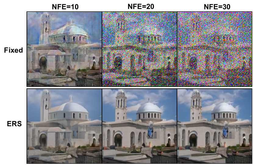
Figure 4: Generation quality comparison between error-robust selection strategy (ERS) with $\lambda=5.0$ and fixed strategy (Fixed) that select the last $k$ estimated noises fixedly based on 5-order Lagrange interpolation function.

Cifar10.

The comparison results on Cifar10 are shown in Tab. 3. Our ERA-Solver achieves better results at 5, 10, 12, 20, and 40 NFEs. When evaluated on 10 NFE, our ERA-Solver obtains 5.14 FID result, achieving a 19.15% improvement compared with the previous best result of 6.37.

4.3 Ablation Study

Effectiveness of error-robust selection strategy.

We compare our error-robust selection strategy and fixed strategy which selects the last $k$ estimated noises ($\tau_{m}=i-m$ in Eq. 13) based on various orders of Lagrange interpolation function in the predictor. The results can be seen in Tab .4. We further visualize the samples generated from two strategies based on a 5-order Lagrange interpolation function, the results of which are shown in Fig. 4.

It is worth mentioning that when Lagrange order is high, baseline method tends to be collapse. It can be attributed to Runge phenomenon in interpolation algorithms, which leads to more error accumulation. Benefited from error-robust strategy, which adaptively introduces low error function bases, the solver can still maintain the comparable generation results with the best method. It can be concluded that our proposed strategy is more effective than intuitive strategies, especially when Lagrange function order is high.

Table 4: FID comparison between error-robust selection strategy (ERS) and fixed strategy (fixed) that select the last k estimated noises fixedly based on various Lagrange function orders ($k=3,4,5,6$). All experiments are conducted on LSUN-Church.

Method$\backslash$ NFE		10	15	20	40	50
ERA-Solver-3	fixed	9.83	8.52	8.72	9.58	9.69
	ERS	10.2	8.03	7.63	8.11	8.37
ERA-Solver-4	fixed	10.56	8.72	8.99	9.89	9.92
	ERS	9.42	7.41	7.39	8.26	8.5
ERA-Solver-5	fixed	26.7	30.36	31.58	10.09	10.12
	ERS	10.85	7.48	7.28	8.26	8.64
ERA-Solver-6	fixed	63.91	191.69	315.6	298.22	182.44
	ERS	13.79	8.41	7.41	8.43	8.7

Effectiveness of error measure.

We compare different power scales based on the proposed error measure and various constants. The results can be seen in Fig. 5. It can be observed that the selection strategy based on our error measure has better performance than those based on the constant scale in general.

5 Discussion

Why FID gets worse when NFE >50.

We can notice that our solver performs worse when NFE increases to 50, especially on LSUN dataset (Tab. 2 and Tab. 1). It can be understood that FID results fluctuate around a value, which is verified on PNDM (Liu et al., 2021).

Why ERA-Solver performs worse on Cifar10.

From Tab. 3, we can notice that ERA-Solver performs slightly worse than DPM-Solver and PNDM when NFE increases, which is different from the results on LSUN. The reason behind it is the resolution of data. Cifar10 has a very low resolution (32 $\times$ 32) while LSUN has a higher resolution (256 $\times$ 256), which means the LSUN dataset is more informative than Cifar10. Thus, the model tends to have lower training error (noise estimation error) when trained on Cifar10, leading to the slightly worse performance of ERA-Solver.

Rationality of selection function.

In this paper, we design the selection function for the error robustness of the sampling solver. The changing trend of noise estimation error with timestep (Fig. 1) inspires us to choose the power function as an error-robust selection function and experiments demonstrate its effectiveness. There may exist a better selection function or a learning-based approach to selecting Lagrange functions and we leave it for future work.

Why ERA-Solver has better error robustness.

We notice that the previous numeric solvers (Liu et al., 2021; Lu et al., 2022a, b; Song et al., 2020a) depend on the assumption that the pretrained diffusion model achieves accurate noise estimation. In this paper, we demonstrate that there exists an obvious estimation error (Fig. 1) from pretrained model, which limits the sampling efficiency of previous fast solvers.

Combined with the Lagrange interpolation as the predictor and an error-robust selection strategy, we show that the Implicit Adams solver has the potential to be error-robust so as to achieve better sampling efficiency. The predictor based on Lagrange interpolation makes sure our solver has the convergence property of the numerical solver (predictor-corrector sampling scheme). The error-robust selection strategy adaptively introduces relatively accurate estimated noises and mitigates the error accumulation in the sampling process. More analysis can be found in Appendix. C.

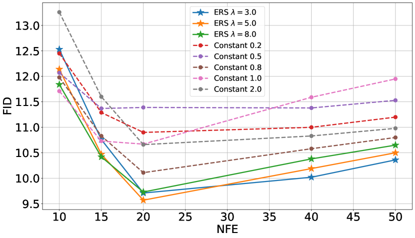
Figure 5: Generation quality measured by FID $\downarrow$. We compare our error-aware scale ($\Delta\epsilon/{\lambda}$ in Eq. 17) and constant scale (replace $\Delta\epsilon/{\lambda}$ with a constant) to demonstrate the effectiveness of the proposed error measure based on the 3-order Lagrange interpolation function. All FID results are evaluated on LSUN-Church with 5000 generated samples.

6 Conclusion

In this paper, we propose an error-robust Adams solver (ERA-Solver) that consists of a predictor and a corrector. We leverage the Lagrange interpolation function to perform the predictor, and further propose an error measure for the sampling process and an error-robust strategy to enhance the predictor. Experiments demonstrate that ERA-Solver achieves better generation quality on LSUN-Church and LSUN-Bedroom datasets at all NFEs. Our ERA-Solver might be misused with powerful diffusion models (Rombach et al., 2022; Kim & Ye, 2021) to generate adverse fake content. We will restrict the usage of our solver and share it with the fake detection community.

Appendix A Ablation Study on Cifar10

In this part, we provide ablation experiments on Cifar10 dataset. We replace our error-robust selection strategy with the fixed selection strategy that fixedly selects the last k estimated noises previously saved in the Lagrange buffer at every sampling step. The results are shown in Tab. 5. From the table, we can see that our selection strategy achieves better FID generation results.

We also conduct ablation studies for proposed error measures in the sampling process. We parameterize the power function with various constants instead of our error measure. The comparison results are shown in Fig. 6. Our error measure can enhance the selection strategy with better generation results in general.

Appendix B Additional Results on Celeba

The comparison results on Celeba are shown in Tab. 6. When tested on a few NFEs like 10 and 12, our ERA-Solver obtains 5.06 and 3.67 FID results, achieving 26.8% and 14.4% improvements compared with the previous best results of 6.92 and 4.20. It can also be observed that FID result of ERA-Solver converges at about NFE 15. Compared with DPM-Solver which converges at NFE 36, ERA-Solver has better convergence speed, while achieving comparable generation quality (FID 2.75 vs 2.71).

Appendix C Analysis of Error Robustness

Since data distributions like LSUN are high-dimensional and complex, it is difficult to seek a ground truth for the predicted noise in the sampling process. Thus, we demonstrate the error robustness of ERA-Solver from another perspective. Assume that we achieve a generated sample $\mathbf{x}_{0}^{gen}$ from a solver, we can utilize the diffusion process to add noise to the sample, remapping the sample obtained from the denoising process back to the noise space to derive $\mathbf{x}_{t}^{gen}$. We measure the error robustness of the solver as the following:

$$||{\boldsymbol{\epsilon}}-{\boldsymbol{\epsilon}}_{\theta}(\mathbf{x}_{t}^{gen},t)||_{2},$$ (18)

The estimated noise from pretrained model can be seen as the stepping direction of the noisy sample (Song et al., 2020b). If a solver is not error-robust, its generated samples will deviate from the original generation path in the sampling process. Since the generation process can be seen as the reverse process of the diffusion process, the deviation of generated samples will increase the error in Eq. 18.

Table 5: FID comparison between error-robust selection strategy (ERS) and fixed strategy (fixed) based on various Lagrange function orders ($k=3,4,5,6$).

Method$\backslash$ NFE		10	15	20	50
ERA-Solver-3	fixed	5.95	4.62	4.24	4.0
	ERS	5.79	4.31	4.07	3.94
ERA-Solver-4	fixed	6.4	4.46	4.1	3.98
	ERS	5.14	3.86	3.79	3.91
ERA-Solver-5	fixed	17.21	15.11	17.47	3.99
	ERS	6.26	3.73	3.69	3.98
ERA-Solver-6	fixed	36.34	51.58	83.39	118.38
	ERS	19.26	4.16	3.73	4.04

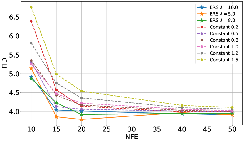
Figure 6: Generation quality measured by FID $\downarrow$. We compare our error-aware scale ($\Delta\epsilon/{\lambda}$) and constant scale based on the 4-order Lagrange function. All FID results are evaluated on Cifar10 with 50k generated samples.

We select normal Implicit Adam solver (Małgorzata & Marciniak, 2006), DPM-Solver (Lu et al., 2022a), and ERA-Solver for comparisons and generate a batch of samples to calculate Eq. 15 separately. Three solvers share the same sampling NFE, random seed, and the pretrained model ${\boldsymbol{\epsilon}}_{\theta}$. The results are shown in Fig. 7, from which we can see that ERA-Solver achieves lower error in general.

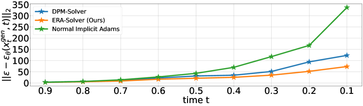
Figure 7: The error comparison between three fast solvers. For ERA-Solver, we set $k=4$ and $\lambda=5.0$. The random seed and pretrained model are shared with three solvers.

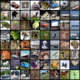
Figure 8: Generated samples from ERA-Solver-4 (20 NFE).

Table 6: Generation quality measured by FID $\downarrow$ on Celeba, varying the number of function evaluation (NFE).

Sampling method $\backslash$ NFE	5	10	12	15	20	40	50	100
DDIM (Song et al., 2020a)	24.26	13.4	13.23	11.63	9.62	6.87	6.08	4.5
Analytic-DDPM (Bao et al., 2022)	$\backslash$	28.99	25.27	21.80	18.14	$\backslash$	11.23	$\backslash$
Analytic-DDIM (Bao et al., 2022)	$\backslash$	15.62	13.90	12.29	10.45	$\backslash$	6.13	$\backslash$
PNDM (Liu et al., 2021)	$\backslash$	$\backslash$	$\backslash$	10.91	7.59	4.06	3.45	2.97
DPM-Solver-fast (Lu et al., 2022a)	$\backslash$	6.92	4.20	3.05	2.82	2.71 (NFE = 36)
ERA-Solver	23.32	5.06	3.67	2.99	2.75	2.69	2.73	2.72

Appendix D Qualitative Results

We sample and visualize the generated samples from LSUN-Church and LSUN-Bedroom datasets. We evaluate DDIM, DPM-Solver, and our method based on 5, 8, 10, 12, 15, and 20 NFEs. Since PNDM (Liu et al., 2021) requires at least 13 NFEs to perform sampling, we only compared our method with DDIM (Song et al., 2020a) and DPM-Solver-fast (Lu et al., 2022a) methods. We set $\lambda=5.0$ and apply a 4-order Lagrange interpolation function ($k=4$) for comparison. The comparison results are shown in Fig. 9 and Fig. 10. Compared with DDIM, our ERA-Solver can obtain sharper textures, benefiting from its high precision of the implicit Adams scheme. Compared with DPM-Solver-fast, our ERA-Solver can avoid excessive contrast and exposure, achieving more natural texture details.

We also provide generated samples based on the 4-order ERA-Solver with $\lambda=5.0$ on Cifar10, as shown in Fig. 8.

Appendix E Results on Stable Diffusion

We conduct generation comparison based on large-scale latent diffusion mode, i.e., Stable Diffusion (Rombach et al., 2022). We apply the improved version (Lu et al., 2022b) of DPM-Solver for better conditional generation. The PNDM and improved DPM-Solver are all encapsulated in diffusers (von Platen et al., 2022). We directly apply them by diffusers to make sampling. For ERA-Solver, we set $k=4$ and $\lambda=10.0$. The results are shown in Fig. 11 and Fig. 12. It can be observed that ERA-Solver can generate promising images when NFE is 15, which is faster than DPM-Solver and PNDM.

Table 7: Computation time of sampling on Stable Diffusion, varying different solvers and NFE.

Sampling Method $\backslash$ NFE	15	25	50
PNDM (Liu et al., 2021)	2.69	3.74	6.13
DPM-Solver (Lu et al., 2022a)	1.86	2.76	5.30
ERA-Solver	1.94	3.05	6.01

We also provide computation time for each sampling process, as shown in Tab. 7. It can be observed that at NFE 15, ERA-Solver consumes slightly more time (0.08s) than DPM-Solver, which can be contributed to the cost of maintaining the Lagrange buffer. The cost of the Lagrange buffer will increase with NFE increasing. However, ERA-Solver has been able to generate exquisite images on NFE 15. Thus, the computation cost of the Lagrange buffer can be ignored.

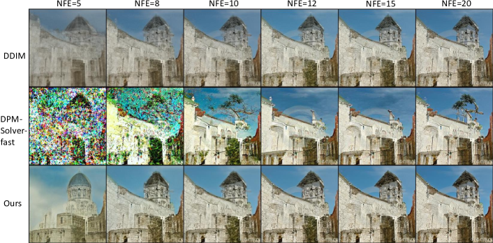
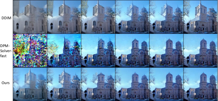
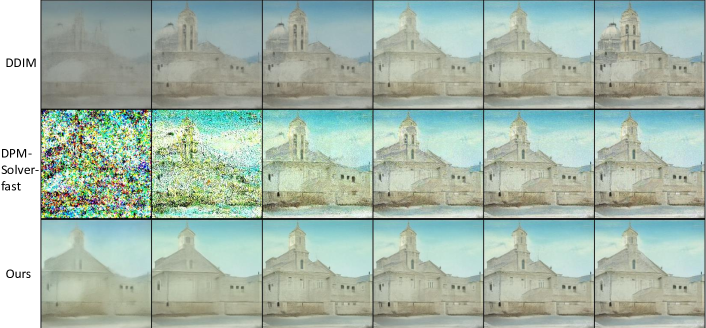
Figure 9: Generation quality comparison with 5, 8, 10, 12, 15, and 20 NFEs on LSUN-Church dataset.

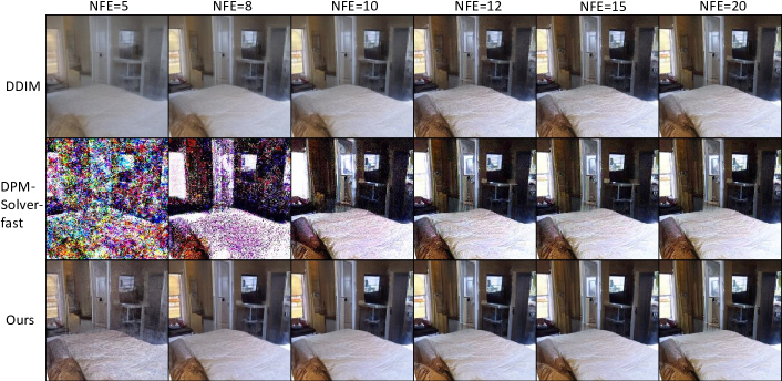
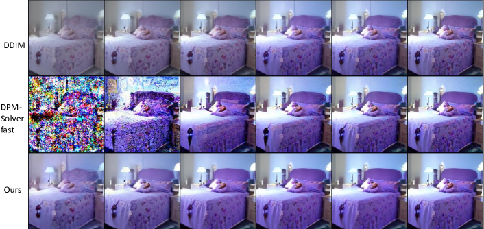
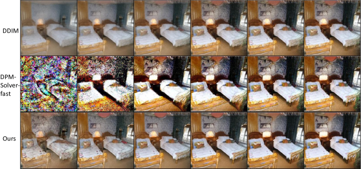
Figure 10: Generation quality comparison with 5, 8, 10, 12, 15, and 20 NFEs on LSUN-Bedroom dataset.

Figure 11: Samples using the pretrained Stable-Diffusion (Rombach et al., 2022) with a classifier-free guidance scale 7.5 (the default setting), varying different solvers and NFEs. The main part of input prompt is: “Cute and adorable ferret wizard, wearing coat and suit”.

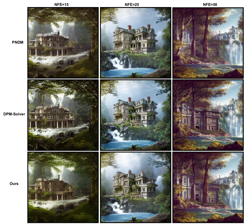
Figure 12: Samples using the pretrained Stable-Diffusion (Rombach et al., 2022) with a classifier-free guidance scale 7.5 (the default setting), varying different solvers and NFEs. The main part of input prompt is: “A beautiful mansion beside a waterfall in the woods”.

References

- Atkinson et al. (2011) Atkinson, K., Han, W., and Stewart, D. E. Numerical solution of ordinary differential equations. John Wiley & Sons, 2011.
- Bao et al. (2022) Bao, F., Li, C., Zhu, J., and Zhang, B. Analytic-dpm: an analytic estimate of the optimal reverse variance in diffusion probabilistic models. arXiv preprint arXiv:2201.06503, 2022.
- Butcher (1996) Butcher, J. C. A history of runge-kutta methods. Applied numerical mathematics, 20(3):247–260, 1996.
- Chen et al. (2022) Chen, W., Hu, H., Saharia, C., and Cohen, W. W. Re-imagen: Retrieval-augmented text-to-image generator. arXiv preprint arXiv:2209.14491, 2022.
- Child (2021) Child, R. Very deep vaes generalize autoregressive models and can outperform them on images. arXiv:2011.10650, 2021.
- Diethelm et al. (2002) Diethelm, K., Ford, N. J., and Freed, A. D. A predictor-corrector approach for the numerical solution of fractional differential equations. Nonlinear Dynamics, 29(1):3–22, 2002.
- Goodfellow et al. (2014) Goodfellow, I. J., Pouget-Abadie, J., Mirza, M., Xu, B., Warde-Farley, D., Ozair, S., Courville, A., and Bengio, Y. Generative adversarial networks. arXiv:1406.2661, 2014.
- Gu et al. (2022) Gu, S., Chen, D., Bao, J., Wen, F., Zhang, B., Chen, D., Yuan, L., and Guo, B. Vector quantized diffusion model for text-to-image synthesis. In Proceedings of the IEEE/CVF Conference on Computer Vision and Pattern Recognition, pp. 10696–10706, 2022.
- Heusel et al. (2017) Heusel, M., Ramsauer, H., Unterthiner, T., Nessler, B., and Hochreiter, S. Gans trained by a two time-scale update rule converge to a local nash equilibrium. Advances in Neural Information Processing Systems 30 (NIPS 2017), 2017.
- Ho et al. (2020) Ho, J., Jain, A., and Abbeel, P. Denoising diffusion probabilistic models. In NeurIPS, 2020.
- Hoogeboom et al. (2022) Hoogeboom, E., Satorras, V. G., Vignac, C., and Welling, M. Equivariant diffusion for molecule generation in 3d. In International Conference on Machine Learning, pp. 8867–8887. PMLR, 2022.
- Huang et al. (2021) Huang, C.-W., Lim, J. H., and Courville, A. C. A variational perspective on diffusion-based generative models and score matching. Advances in Neural Information Processing Systems, 34, 2021.
- Huang et al. (2022) Huang, L., Zhang, H., Xu, T., and Wong, K.-C. Mdm: Molecular diffusion model for 3d molecule generation. arXiv preprint arXiv:2209.05710, 2022.
- Jing et al. (2022) Jing, B., Corso, G., Chang, J., Barzilay, R., and Jaakkola, T. Torsional diffusion for molecular conformer generation. arXiv preprint arXiv:2206.01729, 2022.
- Kawar et al. (2022) Kawar, B., Elad, M., Ermon, S., and Song, J. Denoising diffusion restoration models. arXiv preprint arXiv:2201.11793, 2022.
- Kim & Ye (2021) Kim, G. and Ye, J. C. Diffusionclip: Text-guided image manipulation using diffusion models. 2021.
- Krizhevsky et al. (2009) Krizhevsky, A., Nair, V., and Hinton, G. CIFAR-10 (Canadian Institute for Advanced Research), 2009. URL http://www.cs.toronto.edu/~kriz/cifar.html.
- Lam et al. (2022) Lam, M. W., Wang, J., Su, D., and Yu, D. Bddm: Bilateral denoising diffusion models for fast and high-quality speech synthesis. arXiv preprint arXiv:2203.13508, 2022.
- Leng et al. (2022) Leng, Y., Chen, Z., Guo, J., Liu, H., Chen, J., Tan, X., Mandic, D., He, L., Li, X.-Y., Qin, T., et al. Binauralgrad: A two-stage conditional diffusion probabilistic model for binaural audio synthesis. arXiv preprint arXiv:2205.14807, 2022.
- Liu et al. (2022) Liu, H., Wang, Y., Wang, M., and Rui, Y. Delving globally into texture and structure for image inpainting. In Proceedings of the 30th ACM International Conference on Multimedia, pp. 1270–1278, 2022.
- Liu et al. (2021) Liu, L., Ren, Y., Lin, Z., and Zhao, Z. Pseudo numerical methods for diffusion models on manifolds. In International Conference on Learning Representations, 2021.
- Liu et al. (2015) Liu, Z., Luo, P., Wang, X., and Tang, X. Deep learning face attributes in the wild. In Proceedings of International Conference on Computer Vision (ICCV), December 2015.
- Lu et al. (2022a) Lu, C., Zhou, Y., Bao, F., Chen, J., Li, C., and Zhu, J. Dpm-solver: A fast ode solver for diffusion probabilistic model sampling in around 10 steps. arXiv preprint arXiv:2206.00927, 2022a.
- Lu et al. (2022b) Lu, C., Zhou, Y., Bao, F., Chen, J., Li, C., and Zhu, J. Dpm-solver++: Fast solver for guided sampling of diffusion probabilistic models. arXiv preprint arXiv:2211.01095, 2022b.
- Lugmayr et al. (2022) Lugmayr, A., Danelljan, M., Romero, A., Yu, F., Timofte, R., and Van Gool, L. Repaint: Inpainting using denoising diffusion probabilistic models. In Proceedings of the IEEE/CVF Conference on Computer Vision and Pattern Recognition, pp. 11461–11471, 2022.
- Luo (2022) Luo, C. Understanding diffusion models: A unified perspective. arXiv preprint arXiv:2208.11970, 2022.
- Lyu et al. (2022) Lyu, Z., Xu, X., Yang, C., Lin, D., and Dai, B. Accelerating diffusion models via early stop of the diffusion process. arXiv preprint arXiv:2205.12524, 2022.
- Małgorzata & Marciniak (2002) Małgorzata, J. and Marciniak, A. On explicit interval methods of adams-bashforth type. CMST, 8(2):46–57, 2002.
- Małgorzata & Marciniak (2006) Małgorzata, J. and Marciniak, A. On two families of implicit interval methods of adams-moulton type. CMST, 12(2):109–113, 2006.
- Mohazzabi & Becker (2017) Mohazzabi, P. and Becker, J. L. Numerical solution of differential equations by direct taylor expansion. Journal of Applied Mathematics and Physics, 5(3):623–630, 2017.
- Poole et al. (2022) Poole, B., Jain, A., Barron, J. T., and Mildenhall, B. Dreamfusion: Text-to-3d using 2d diffusion. arXiv preprint arXiv:2209.14988, 2022.
- Rombach et al. (2022) Rombach, R., Blattmann, A., Lorenz, D., Esser, P., and Ommer, B. High-resolution image synthesis with latent diffusion models. In Proceedings of the IEEE/CVF Conference on Computer Vision and Pattern Recognition, pp. 10684–10695, 2022.
- Salimans & Ho (2021) Salimans, T. and Ho, J. Progressive distillation for fast sampling of diffusion models. In International Conference on Learning Representations, 2021.
- Sauer & Xu (1995) Sauer, T. and Xu, Y. On multivariate lagrange interpolation. Mathematics of computation, 64(211):1147–1170, 1995.
- Song et al. (2020a) Song, J., Meng, C., and Ermon, S. Denoising diffusion implicit models. arXiv:2010.02502, 2020a.
- Song et al. (2020b) Song, Y., Sohl-Dickstein, J., Kingma, D. P., Kumar, A., Ermon, S., and Poole, B. Score-based generative modeling through stochastic differential equations. arXiv:2011.13456, 2020b.
- von Platen et al. (2022) von Platen, P., Patil, S., Lozhkov, A., Cuenca, P., Lambert, N., Rasul, K., Davaadorj, M., and Wolf, T. Diffusers: State-of-the-art diffusion models. https://github.com/huggingface/diffusers, 2022.
- Wang et al. (2022) Wang, Z., Zheng, H., He, P., Chen, W., and Zhou, M. Diffusion-gan: Training gans with diffusion. arXiv preprint arXiv:2206.02262, 2022.
- Watson et al. (2021) Watson, D., Chan, W., Ho, J., and Norouzi, M. Learning fast samplers for diffusion models by differentiating through sample quality. In International Conference on Learning Representations, 2021.
- Wells (1982) Wells, D. R. Multirate linear multistep methods for the solution of systems of ordinary differential equations. University of Illinois at Urbana-Champaign, 1982.
- Wu et al. (2022) Wu, L., Gong, C., Liu, X., Ye, M., and Liu, Q. Diffusion-based molecule generation with informative prior bridges. arXiv preprint arXiv:2209.00865, 2022.
- Yu et al. (2015) Yu, F., Seff, A., Zhang, Y., Song, S., Funkhouser, T., and Xiao, J. Lsun: Construction of a large-scale image dataset using deep learning with humans in the loop. arXiv:1506.03365, 2015.