A strong X-ray polarization signal from the magnetar 1RXS J170849.0-400910

Abstract

Magnetars are the most strongly magnetized neutron stars, and one of the most promising targets for X-ray polarimetric measurements. We present here the first Imaging X-ray Polarimetry Explorer (IXPE) observation of the magnetar 1RXS J170849.0-400910, jointly analysed with a new Swift observation and archival NICER data. The total (energy and phase integrated) emission in the 2–8 keV energy range is linerarly polarized, at a $\sim 35$% level. The phase-averaged polarization signal shows a marked increase with energy, ranging from $\sim$ 20% at 2–3 keV up to $\sim$ 80% at 6–8 keV, while the polarization angle remain constant. This indicates that radiation is mostly polarized in a single direction. The spectrum is well reproduced by a combination of either two thermal (blackbody) components or a blackbody and a power law. Both the polarization degree and angle also show a variation with the spin phase, and the former is almost anti-correlated with the source counts in the 2–8 keV and 2–4 keV bands. We discuss the possible implications and interpretations, based on a joint analysis of the spectral, polarization and pulsation properties of the source. A scenario in which the surface temperature is not homogeneous, with a hotter cap covered by a gaseous atmosphere and a warmer region in a condensed state, provides a satisfactory description of both the phase- and energy-dependent spectro-polarimetric data. The (comparatively) small size of the two emitting regions, required to explain the observed pulsations, does not allow to reach a robust conclusion about the presence of vacuum birefringence effects.

=400

1 Introduction

The launch of the NASA-ASI Imaging X-ray Polarimetry Explorer (IXPE; Weisskopf et al., 2022) in December 2021 opened a new window to our view of the X-ray sky by adding polarimetry to spectroscopy, timing and imaging as a tool to interpret astrophysical X-ray sources. IXPE has been in operation for nearly one year now, and already observed more than $30$ X-ray sources belonging to different classes.

Particularly interesting for IXPE observations are magnetars, a class of isolated neutron stars (NSs) that are powered by their huge magnetic field Duncan & Thompson (1992); Thompson & Duncan (1993). They are characterized by an X-ray luminosity $L\approx 10^{31}$–$10^{36}$ erg s^-1, spin period $P\approx 1$–$12$ s, and period derivative $\dot{P}\approx 10^{-13}$–$10^{-11}$ s s^-1, implying a dipole field $B\approx 10^{14}$–$10^{15}$ G. Magnetars are extremely active sources over different ranges of luminosities and timescales, from the short-lived X-ray bursts and powerful giant flares to outbursts, during which their persistent X-ray flux suddenly increases by a factor of $\approx 10$–$1000$ and then gradually decays over months/years (e.g. Rea & Esposito, 2011; Coti Zelati et al., 2018).

Magnetar X-ray spectra below $10$ keV are typically well reproduced by a two-component model, comprising either two thermal (blackbody, BB) components or a thermal component plus a non-thermal (power-law, PL) one. While the BB component(s) is believed to originate from (regions of) the cooling star surface, the PL one is usually interpreted as due to resonant cyclotron scattering (RCS) of thermal photons off magnetospheric currents flowing in a twisted magnetic field. In addition, magnetars exhibit a powerful and highly pulsed non-thermal emission at higher energies, up to $\sim 100$–$200$ keV, first discovered by INTEGRAL (see e.g. Turolla et al., 2015; Kaspi & Beloborodov, 2017, for reviews).

Strongly magnetized sources, which electromagnetic emission is expected to be highly polarized, are ideal targets for X-ray polarimetry. Emission from highly magnetized neutron stars is expected to be linearly polarized in two normal modes, the ordinary (O) and extraordinary (X) ones, with the polarization electric vector either parallel or perpendicular to the plane of the photon direction and the (local) magnetic field. The degree of polarization depends on the properties of the emission region, its geometry, magnetic field strength and orientation, and on the dominant radiative processes. This makes X-ray polarimetry a new, powerful tool to probe the magnetospheric topology of the magnetar, the state of matter in the star crust, including whether the star has a bare, condensed surface or is surrounded by a gaseous atmosphere (see e.g. Taverna et al., 2020; Caiazzo et al., 2022, and references therein), and even to test the properties of the QED magnetized vacuum around the star, such as its birefringence (Heyl & Shaviv, 2000, 2002).

IXPE first observed a magnetar source, the bright Anomalous X-ray Pulsar (AXP) 4U 0142+61, in February 2022. The polarization signal was clearly detected at $\sim 13\%$ level, with both the polarization degree and angle exhibiting a strong dependence on the energy Taverna et al. (2022). In this paper we report on the IXPE observation of a second magnetar, the AXP 1RXS J170849.0-400910.

2 Source properties and observations

1RXS J170849.0-400910  (1RXS J1708 hereafter) was first identified in the ROSAT All Sky Survey Voges et al. (1999), but only a few years later $\sim 11$ s pulsations were discovered by ASCA Sugizaki et al. (1997). Both the large period derivative ($\dot{P}\sim 2\times 10^{-11}$ s s^-1) and the upper limits inferred for a possible optical counterpart confirmed the source to be a member of the magnetar class Israel et al. (1999). The value of the period derivative, if interpreted as due to a rotating dipole in vacuum, yields a dipole magnetic field strength of $\sim 4-5\times 10^{14}$ G. The source presents an erratic timing behavior, characterized by frequent glitching activity that interrupt periods of steady spin-down Dib & Kaspi (2014). The X-ray spectrum has been fitted with an absorbed BB+PL model, with (slightly variable) photon index $\Gamma\sim 2.6$ and blackbody temperature $kT\sim 0.45$ keV Rea et al. (2003, 2007); Krawczynski et al. (2022). The source is radio-quiet. Hard, strongly pulsed X-ray emission extending up to $\sim$ 150 keV has been detected from 1RXS J1708 with INTEGRAL Kuiper et al. (2006); a marked variability in the hardness ratio is also observed (Götz et al., 2007).

The distance of the source is uncertain. 1RXS J1708 lies in the Galactic plane, and the large column density inferred from X-ray data, $n_{\mathrm{H}}\sim 1.36\times 10^{22}\ \rm{cm}^{-2}$, suggests a distance in the $5$–$10$ kpc range Israel et al. (1999); Rea et al. (2007), although a smaller value cannot be ruled out, as hinted from spectral fits with atmospheric models or from reddening measures based on 2MASS stars Perna et al. (2001); Durant & van Kerkwijk (2006). In this paper we present the results from the IXPE  observation of 1RXS J1708  performed from 2022-09-19 05:08 UTC to 2022-09-29 12:00 UTC and from 2022-09-30 12:52:02 UTC to 2022-10-08 11:17:40 UTC. We complemented the analysis with data from a Swift-XRT (Burrows et al., 2005) target of opportunity observation, performed on 2022-10-20 for a total of $1020\,\mathrm{s}$, and with the most recent NICER (Arzoumanian et al., 2014) data publicly available (see Appendix A for details). Our observations and the methods used for data processing are described in Appendix A.

3 Phase-integrated polarimetric and spectropolarimetric analysis

No variations in either the source or background were found during the two IXPE observations (see Appendix A.1), therefore the combined data are used in the following analysis. The phase integrated and energy integrated polarization in the $2.0$–$8.0$ keV interval, which is the nominal IXPE energy range, is shown in Figure  1 (left panel) for each detector unit (DU), and for their combination. The values of the Stokes parameters were derived with the ixpeobssim suite (Baldini et al., 2022), and they are weighted by the (energy-dependent) effective area of the instrument. This allows us to correct the measured polarization, which is convolved with the spectral response of the instrument, and to obtain the polarization of the incoming radiation. The circles and the radial lines in Figure 1 mark the loci of constant polarization degree, $\mathrm{PD}=\sqrt{Q^{2}+U^{2}}/I$ and polarization angle, $\mathrm{PA}=\arctan{(U/Q)}/2$, respectively. Since the Stokes parameters are (quasi) normally distributed, we report the one-dimensional uncertainties at 68.3% confidence level ($1\,\sigma$).

The measured polarization angle is $\sim$ 60^∘ West of North, and the phase- and energy-integrated polarization degree is remarkably high, $\sim 35\%$, that is more than 2.5 times the average X-ray polarization of the only other magnetar observed to date (Taverna et al., 2022).

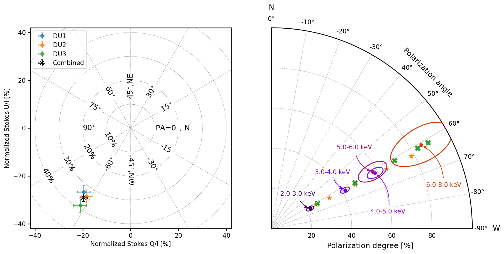
Figure 1: Left: Phase- and energy-averaged linear polarization of 1RXS J1708, in terms of the normalized Stokes parameters. Uncertainties are shown at the 68.3% ($1\,\sigma$) confidence level. Circles with center in the origin and increasing radii correspond to increasing values of the polarization degree while different values of the azimuth to different polarization angles. Right: Polarization of 1RXS J1708 in different energy bands, computed with ixpeobssim. Contours identify the 50% confidence regions for the joint measurement of the polarization degree and angle (which are not independent variables), accounting for statistical fluctuations only. Orange stars and green crosses show, for the same energy bins, the prediction of the belt+cap and cap+cap models, respectively (see §5 for details)

Even higher polarization degrees are detected by binning the data in five energy intervals, as reported in the right panel of Figure 1; here the contours show the 50% confidence regions in the polarization degree vs. polarization angle plane (see also Table 1). The polarization degree increases from $\sim 20\%$ between $2$ and $3$ keV to $\sim 80\%$ in the $6$–$8$ keV energy range. The polarization angle remains roughly constant in all energy bins.

	2–3 keV	3–4 keV	4–5 keV	5–6 keV	6–8 keV	2–8 keV
PD - sum [%]	21.7${}^{+1.7}_{-1.7}$	41.3${}^{+2.0}_{-2.0}$	58.6${}^{+3.7}_{-3.7}$	57.7${}^{+6.8}_{-6.8}$	85${}^{+15}_{-15}$	35.1${}^{+1.6}_{-1.6}$
PD S/N	12.9 $\sigma$	20.2 $\sigma$	15.8 $\sigma$	8.5 $\sigma$	5.8 $\sigma$	22.5 $\sigma$
PA - sum [deg]	$-62.6^{+2.2}_{-2.2}$	$-62.4^{+1.4}_{-1.4}$	$-61.8^{+1.8}_{-1.8}$	$-60.7^{+3.3}_{-3.3}$	$-60.8^{+4.7}_{-4.7}$	$-62.1^{+1.3}_{-1.3}$

Table 1: Values of the measured polarization degree and angle, obtained with the ixpeobssim software suite. Reported values correspond to the sum of the three DUs (the measures of the single DUs are consistent with each other within errors). Uncertainties are obtained at 68.3% confidence level, assuming that the polarization degree and angle are independent. Signal-to-noise is calculated by dividing the polarization degree obtained by combining the results of the three telescopes on-board IXPE  by its uncertainty.

We performed a spectropolarimetric analysis making use of the IXPE, Swift-XRT and NICER observations (the latter performed within a month; see Appendix A). We extracted Swift and NICER energy spectra with the standard data analysis tools and used ixpeobssim to derive the IXPE $I$, $Q$ and $U$ energy spectra. We use XSPEC (version: 12.13.0, Arnaud 1996) for a joint spectropolarimetric fit of the $I$ spectra from all three observatories and the $Q$ and $U$ spectra from IXPE.

We tested two models commonly used to interpret magnetar soft X-ray spectra, i.e. an absorbed BB+PL and a BB+BB. We started with the BB+PL model, multiplying the BB and PL components with a polarization factor constant in energy; the corresponding XSPEC model is TBabs*(bbody * polconst + powerlaw * polconst), with abundances from Wilms et al. (2000). We include multiplicative constant factors for each IXPE DU and for each observatory, except for IXPE DU1 which is used as reference. The fit gives a statistically acceptable $\chi^{2}=410.4$ for $408$ degrees of freedom (Figure 2). The best-fit parameter values are reported in Table 2 in Appendix B. Our fit parameters are in approximate agreement with those reported in Rea et al. (2007). The different neutral hydrogen column densities ($n_{\mathrm{H}}\sim 2\times 10^{22}\ \mathrm{cm}^{-2}$ instead of $\sim 1.4\times 10^{22}\ \mathrm{cm}^{-2}$) largely result from the use of a different absorption model and elemental abundances, TBabs and Wilms et al. (2000) in our case instead of phabs and Anders & Grevesse (1989). We find however a significantly steeper PL than Rea et al. (2007). The PL component dominates over the BB component at all energies, the latter contributing only $\sim 20\%$ in the 2–8 keV energy range (see Fig. 2).

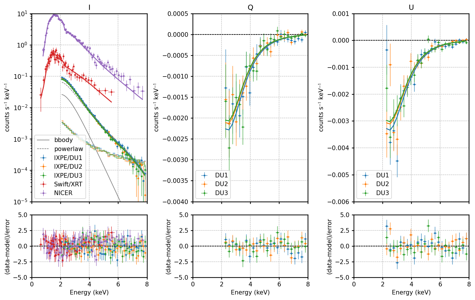
Figure 2: Joint spectropolarimetric fit of IXPE, Swift/XRT and NICER data. The Stokes $I$, $Q$ and $U$ energy spectra are obtained by binning the event-by-event Stokes parameters, calculated following Kislat et al. (2015), according to the measured energy of the event. $Q$ and $U$ are given by the source flux multiplied by the polarization degree and either the cosine or the sine of twice the polarization angle, respectively. The Stokes $I$, $Q$ and $U$ energy spectra convolved with the instrument response are shown in the left, central and right panels, respectively. The best-fit model of the form TBabs*(bbody * polconst + powerlaw * polconst) is shown by the solid lines. Fit residuals are shown in the bottom panels; see Table 2 in Appendix B for the fit parameters. Light colored curves are the background of IXPE detectors.

The simultaneous fit of the $Q$ and $U$ energy spectra provides further insights. We find that the PA associated to the BB component turns out to be different by $\sim 90^{\circ}$ with respect to that of the PL. This is similar to what IXPE observed in 4U 0142+61 (Taverna et al., 2022), and it supports a scenario in which thermal and non-thermal photons are polarized, one in the X and the other in the O mode. The changing polarization degree with energy can be then explained as due to the different relative contributions of the two orthogonally polarized components. However, the polarization degree turns out to be much higher in 1RXS J1708 than in 4U 0142+61. Taken at face value, the best fit gives a 100% polarized blackbody component (see Table  2 in Appendix B). However, the polarization properties of this component are not well constrained and, for instance, fixing the polarization degree of the BB component to 20% still gives an acceptable fit ($\chi^{2}=434.2$ for $408$ degrees of freedom). We infer that the PL component is linearly polarized to $\sim$ 65–75%, depending on the polarization of the blackbody component. This polarization degree is much higher than predicted by the resonant scattering scenario (Taverna et al., 2022). It should be noted that the assumptions of constant thermal and power law polarization degrees lead to a significant contribution of the thermal component. The data can be fit with a single PL component if we allow for a polarization degree with a linear energy dependence (we get a $\chi^{2}=454.3$ for $410$ degrees of freedom for a power law fit with a photon index of $3.43\pm 0.02$; the probability for getting higher $\chi^{2}$ values by chance is $\sim 6\%$).

In the next step, we fitted the data with an absorbed BB+BB model, again assuming a constant polarization for each additive component; the correspondent XSPEC model is TBabs*(bbody * polconst + bbody * polconst). The result of the fit is shown in Figure 3 (see again Appendix A, Table 2). Also in this case, the fit is acceptable ($\chi^{2}=405.8$ for $408$ degrees of freedom) and the high-energy BB component is highly polarized, $\sim$ 70%. The low-energy component is polarized parallel to the high-energy component. The best-fit model exhibits low polarization in the cold BB component, and by fixing the polarization degree to $\sim$ 20% also provides an acceptable fit with $\chi^{2}=422.5$ for 409 degree of freedom. It is worth noting that requiring a low-energy polarization angle orthogonal to the high-energy polarization angle gives a low-energy polarization degree consistent with zero. Therefore, in this scenario, the observed increase of polarization with energy stems from the superposition of two parallel polarized components, a weakly polarized component dominating at low energies and a strongly polarized component dominating at high energies, in the IXPE range.

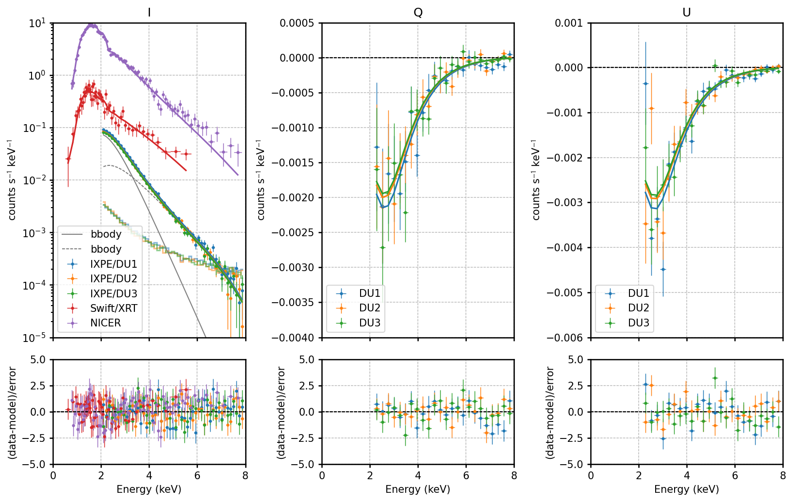
Figure 3: Same as in Figure 2, for the TBabs*(bbody * polconst + bbody * polconst) model. See Table 2 in Appendix B for the fit parameters.

4 Phase-resolved spectropolarimetric analysis

The first step of our phase-resolved analysis involved the determination of an accurate timing solution of the count rate data (see Appendix C). Using epoch MJD 59850.84175 (TDB) as a reference, this provided $f= 0.090795742(5)$ Hz, $\dot{f}=-1.87(25)\times 10^{-13}$ Hz s^-1. The addition of the second frequency derivative did not improve the fit significantly. We then used this timing solution to perform the phase-resolved analysis. To this aim, we selected photons coming from different rotational phases, and repeated the procedures of Section 3 with the event files of the different phase bins. Rotational phases were ascribed to single events starting from their arrival times using the ixpeobssim tool xpphase, and events in the same phase bins were then added together with the tool xpselect. Results are shown in Figure 4 for the total ($2$–$8$ keV), low ($2$–$4$ keV) and high ($4$–$8$ keV) energy bands. The source flux exhibits a single-peaked, nearly sinusoidal profile, as already reported by Rea et al. (2003); the pulse shape and the pulsed fraction change with energy. The polarization degree and angle also vary with phase, and their pulse profiles are different in different energy bands. The pulse of the polarization degree is broadly anti-correlated with that of the flux both in the total ($2$–$8$ keV) and low ($2$–$4$ keV) energy bands.

On the other hand, in the high energy interval ($4$–$8$ keV) the modulation of the signal is less significant and no robust conclusion can be reached whether this anti-correlation holds at these energies as well.

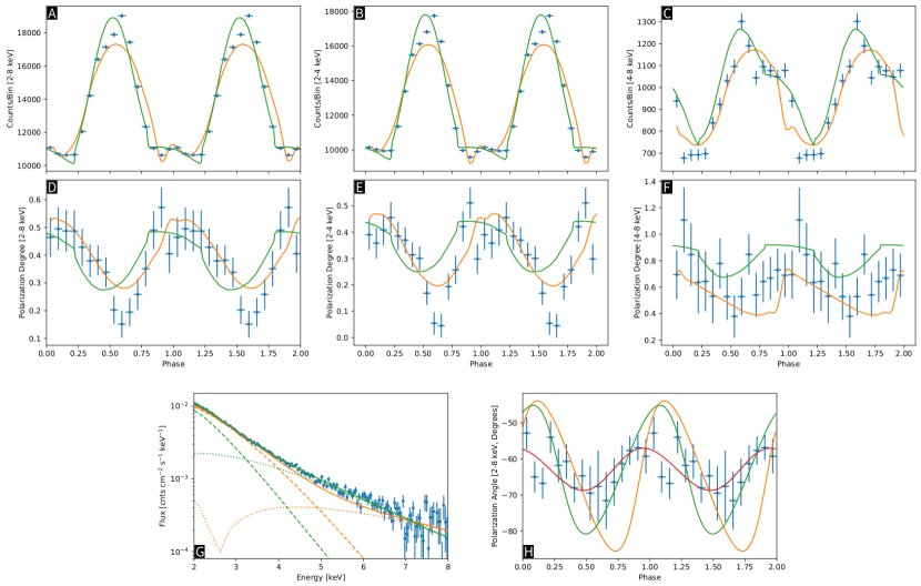
Figure 4: 1RXS J1708 IXPE observation (blue circles with error bars) for the source counts (panels A to C) and polarization degree (panels D to F), plotted as a function of the rotational phase (in each row, the three panels from the left to the right show the data integrated over the $2$–$8$ keV, $2$–$4$ keV and $4$–$8$ keV bands, respectively). Panels G and H show: (left) the phase averaged spectrum (solid lines) together with the contributions of the condensed zone (dashed lines) and atmospheric zone (dotted lines); (right) the polarization angle as a function of the rotational phase, integrated over the 2–8 keV band. Errors are shown at the 1 $\sigma$ level assuming the polarization degree and polarization angle are not correlated. In all panels the orange and green lines represent the model expectation within the belt+cap and cap+cap scenarios (solid lines for the total model, dotted and dashed lines in panel G only for the two separate components); the red solid line in panel H shows the RVM (see the text for the parameter values and other details). Note that data points in the phase-resolved analysis are obtained with ixpeobssim, and therefore independent on the spectral decomposition.

5 Discussion

1RXS J1708 and the Vela PWN Xie et al. (2022) are the most strongly polarized IXPE sources detected so far. The polarization degree of the phase-integrated emission of 1RXS J1708 increases from $\sim 20\%$ around $2$ keV to $\sim 80\%$ at $7$–$8$ keV. The polarization angle, on the other hand, stays roughly constant at $\sim 60^{\circ}$ (counted West of North). The polarimetric properties of 1RXS J1708 are quite at variance with those of the other magnetar observed by IXPE. For both sources, a BB+PL and a BB+BB model provide a satisfactory fit of the IXPE spectrum (see §3). However, 4U 0142+61 exhibits a lower polarization degree which decreases to approximately zero at $\sim 5$ keV, where the polarization angle swings by $90^{\circ}$, and then increases to $\sim 35\%$ around $8$ keV Taverna et al. (2022).

The swing of polarization angle by $90^{\circ}$ and the presence of a power-law tail at higher energies with a value of polarization degree close to $30\%$ led Taverna et al. (2022) to suggest that the X-ray emission from 4U 0142+61 is in two different normal modes below and above $\sim 5$ keV. One possibility that has been suggested is that the low-energy photons are mostly polarized in the O mode and come from either a heated equatorial belt on the condensed neutron star surface or an atmospheric zone which is hit by back-flowing, bombarding magnetospheric currents González-Caniulef et al. (2019), while the high-energy ones are mainly in the X mode being reprocessed by magnetospheric RCS.

The picture for 1RXS J1708 is different. The very high degree of polarization observed at higher energies can not be reproduced by the RCS mechanism, which indicates that RCS is not present, or, at least, that it does not affect primary photons much in the IXPE energy range. The lack of a swing in the polarization angle points to the emission in the $2$–$8$ keV range being dominated by a single mode. The relative contribution of the other mode is larger at lower energies, explaining the lower polarization degree at lower energies. If we assume that radiation comes from the magnetar surface, a polarization degree as large as $\sim 70$–$80\%$ (as that observed at high energies) can be obtained if the star is covered (at least in part) by an atmosphere (e.g. González Caniulef et al., 2016; Taverna et al., 2020; Caiazzo et al., 2022). Emission, then, would be thermal and so the most likely spectral model, among those compatible with the data (see §3), is the BB+BB one. Standard atmospheric emission, however, is hard to reconcile with a polarization degree as low as $\sim 20\%$ (unless the viewing geometry is very particular), as it is observed in 1RXS J1708 at low energies. It is nevertheless possible that, because of a non-homogeneous temperature distribution, some regions of the star surface are cold enough to undergo a phase transition that turns the atmosphere into a magnetic condensate. Emission from the condensed surface can be either in the X or in the O mode but the PD is always modest, $\lesssim 20\%$, and, if the condensate coexists with a hotter region that has an atmosphere on top, this could explain the IXPE observation of 1RXS J1708.

To explore this scenario, we ran a number of simulations assuming that the star surface comprises a hot atmospheric patch at temperature $T_{\rm hot}$ and a warm condensed region at $T_{\rm warm}$; the rest of the surface is again condensed but at a much colder temperature $T_{\rm cold}$. We tried several different geometries, leaving as free parameters the inclination of the line-of-sight, $\chi$, and of the magnetic axis, $\xi$, with respect to the spin axis. This, necessary oversimplified, picture is mostly meant to suggest possibilities on how the main feature of a complex thermal map may look like, and not to provide a diagnostics of the shape and location of the emitting regions.

The emission from the condensate is treated in the free-ion limit and for a Fe composition, following Potekhin et al. (2012). The lack of observed spectral features in the soft X-rays argues against the presence of a heavy-elements atmosphere (see the models by Mori & Ho, 2007, for $B=10^{12}$–$10^{13}$ G). On the other hand, a light elements composition (mostly hydrogen) may be expected if the star experienced episodes of accretion/fallback. We computed emission from a pure hydrogen, completely ionized atmosphere using the numerical setup described in Lloyd (2003). No mode conversion is assumed at the vacuum resonance (see e.g. Ho & Lai, 2003). Photons were then propagated to the observer by using a ray-tracing method. The effects of vacuum birefringence as photons cross the star magnetosphere are accounted for.

We tested various configurations and found that there exist at least two geometrical set-ups, within the scenario outlined above, that match well most of the observed properties of 1RXS J1708. The first one (model A, or “belt plus cap”) is a variation of the geometry envisaged for 4U 0142+61 Taverna et al. (2022), in which the warm (condensed) region corresponds to an equatorial belt, and the hot (atmospheric) region to a circular, polar cap; the belt, however, needs to be limited in azimuth in order to reproduce the X-ray pulse profile. In this case, calculations have been performed using the general relativistic ray-tracing code discussed in Zane & Turolla (2006, see also ). In the second model (model B, or “cap plus cap”) the warm and hot regions are two circular spots, with the warm (condensed) one located about $150^{\circ}$ from the spin axis, and a hot (atmospheric) spot located in the opposite hemisphere and displaced in longitude by about $90^{\circ}$ with respect to the warm one. For this latter scenario, we used the spectro-polarimetric magnetar model discussed in Caiazzo et al. (2022), properly extended to account for different circular regions. We refer to the original papers for a detailed description of the models and the meaning of the various parameters.

We found that the values of the parameters that best match the data are similar in the two cases: $T_{\rm hot}\sim 0.8$ keV, $T_{\rm warm}\sim 0.6$ keV (all values are referred to the star surface), and a magnetic field of $\sim 10^{14}$ G (model B) or $\sim 5\times 10^{14}$ G (model A). Also the values of the geometrical viewing angles are comparable, $\chi\sim 30^{\circ}$ and $\xi\sim 10^{\circ}$. The size of the emitting regions turns out to be somewhat smaller for model B, semi-aperture $\sim 5^{\circ}$ vs. $\sim 10^{\circ}$ for the atmospheric cap and semi-aperture $\sim 22^{\circ}$ of the warm cap as compared to $\sim 30^{\circ}\times 270^{\circ}$ of the belt. The observed pulsations require the size of the emitting regions to be relatively small, and this place an upper limit on the source distance to about 5 kpc.

QED vacuum birefringence can strongly affect the polarization properties at infinity, leading to an enhancement in the polarization degree of the observed signal. However, the extent to which QED effects are measurable is actually quite sensitive to the size of the radiating region on the star surface. As discussed in van Adelsberg & Perna (2009), if emission comes from a small polar cap, the depolarization due to geometrical effects is not present, so that expectations from models computed with or without vacuum birefringence are quite the same. In the case of 1RXS J1708  the small size of the two emitting regions (in particular that of the hot, highly polarized spot) does not allow for a robust test of vacuum birefringence.

Both these models can reproduce the main spectropolarimetric features observed in 1RXS J1708 by IXPE: namely the spectrum; the energy dependence of the phase-averaged polarization degree and angle across the $2$–$8$ keV band (see Fig. 1); the pulse profile in the entire IXPE range ($2$–$8$ keV), and in the $2$–$4$ and $4$–$8$ keV bands; the energy integrated polarization degree as a function of phase in the total, $2$–$4$ and $4$–$8$ keV ranges, including the anti-correlation in phase of the polarization degree and the flux in the total and low-energy bands (see Figure 1). As it can be seen in the panel H of Figure 4, the observed amount of swing in the polarization angle with phase can also be explained by both models; the red curve depicts the best-fit simple rotating vector model (RVM; with unbinned likelihood analysis, e.g. González-Caniulef et al., 2022). In both the proposed configurations model spectra show no features, in agreement with data (see Figure 4). In principle absorption features are expected in the spectrum of a pure hydrogen atmosphere or in that of the magnetic condensate. However, the strong proton cyclotron line in the atmospheric component is $\sim 0.6$ keV in model B, and is drowned out by the dominant contribution from the colder belt in model A. Emission from the condensate component predicts spectral features at low energies ($\sim 0.6$ keV) but, at least for these model parameters, they are too faint to be detectable in the currently available spectra.

The observed anti-correlation in phase of the polarization degree and the flux is due to the relative dominance of two regions, and to the fact that the (less polarized) condensed zone is contributing to much of the counts below $\sim 4$ keV.

There are, however, some caveats. The surface temperature of the warm condensed region is very close to that of the hotter atmospheric patch. Although the conditions for a phase transition in a strongly magnetized medium are still largely uncertain, assuming a dipolar magnetic field with polar strength $\sim 5\times 10^{14}$ G, condensation is expected at $T\lesssim 0.5$ and $T\lesssim 0.9$ keV at the equator and the pole, respectively, for a Fe composition (Medin & Lai, 2007, see also figure 1 in Taverna et al. 2020). This may indicate that, if the hot and warm regions at the star surface, which are in different phases, have the same chemical composition, they are very close to the phase transition. Alternatively, it may indicate that the chemical composition varies across the surface (as in our models, which assume a pure hydrogen atmosphere and an iron condensate), that the real surface temperature map is more complicated than what is caught in our, necessarily, oversimplified model, or that there may be departures of the local magnetic field from the (overall) dipole topology.

As mentioned before, the spectro-polarimetric analysis indicates that the data are also compatible with a scenario in which emission is dominated by a non-thermal (PL) component. Would that be the case, the fact that the polarization degree decreases at low energies may be due either to the presence of a second sub-dominant spectral component with emission in the opposite polarization mode (e.g. a thermal emission from a condensed part of the crust) or to the fact that the non-thermal emission has an intrinsic variation of the polarization properties with energy. The main reason why we have not attempted to explore this scenario is that the very high degree of polarization observed at high energy ($\sim 70-80\%$ ) cannot be reconciled with the physical models commonly proposed to explain the non-thermal emission from magnetars in the soft X-ray band, e.g. RCS (saturated RCS only predicts a $\sim 30\%$ level of polarization). However, it is worth noticing that 1RXS J1708 exhibits a strong non-thermal emission at high energies, as detected in the INTEGRAL band, with extreme variations in phase and energies, whose origin is still unexplained in terms of detailed physical models Kuiper et al. (2006). It could therefore be possible that this non thermal component and that observed in the IXPE band could be similar in origin (but with varying degrees of manifestation).

Appendix A Observational data and data processing

A.1 IXPE

IXPE  observed 1RXS J1708 in two segments close in time, from 2022-09-19 05:08 UTC to 2022-09-29 12:00 UTC and from 2022-09-30 12:52:02 UTC to 2022-10-08 11:17, for a total livetime of $\sim 837$ ks. Level 2 (LV2) data, processed to produce suitable inputs for science analysis, were downloaded from the IXPE archive at HEASARC. One file for each of the three IXPE telescopes was generated, and they were further processed independently. Photons arrival times are corrected to the solar system barycenter in the Barycentric Dynamical Time (TDB) scale, with the FTOOL/barycorr tool, included in HEASOFT 6.31, using the object coordinates stored in the LV2 file, the Jet Propulsion Laboratory Development Ephemeris 421 and the International Celestial Reference System reference frame. Background events in the LV2 files are at first partially rejected. They are identified starting from topological characteristics of the event, e.g., the number of hit pixels and the fraction of the energy in the main track with respect to the total collected for the event. Events falling outside pre-defined intervals are tagged as background and removed. This approach allows to reduce the background counting rate by more then $30\%$, at the cost of a reduction of the source count rate by $\sim 0.5\%$, which is deemed negligible for the subsequent analysis (see Di Marco et al., 2023, for a more detailed description).

The source region is then defined with SAOImage DS9 (Joye & Mandel, 2003) as a circle with radius of 1.5 arcmin. The background is extracted from an annulus centered on 1RXS J1708 with inner and outer radii of 2.5 and 4.0 arcmin, respectively. Response to polarization is extracted from LV2 data with the ixpeobssim  package (Baldini et al., 2022), which implements the algorithms in Kislat et al. (2015) and is publicly available. Spectro-polarimetric analysis is carried out by feeding the Stokes spectra, generated with the ixpeobssim tool xpbin, into XSPEC (Arnaud, 1996) and exploiting the appropriate response matrices available at HEASARC for modelling the polarization as suggested by Strohmayer (2017). The light curve of 1RXS J170849.0-400910 and of the background during the two IXPE observations is shown in Figure 5. Note that the first segment is splitted in two pointings, the first between 19-09-2022 5.00 - 7:20 UTC and the second starting at 19-09-2022 17:30 and ending at 29-09-2022 12:00. Both components did not show any indication of either a spectral or polarization variation with time. To test this, we binned the lightcurves of the Stokes parameters and background in bins of 20ks and we checked that the variations are compatible with statistical fluctuations only (the null probabilty for a fit with a constant is acceptable). Therefore, we proceeded with the analysis by summing all the data.

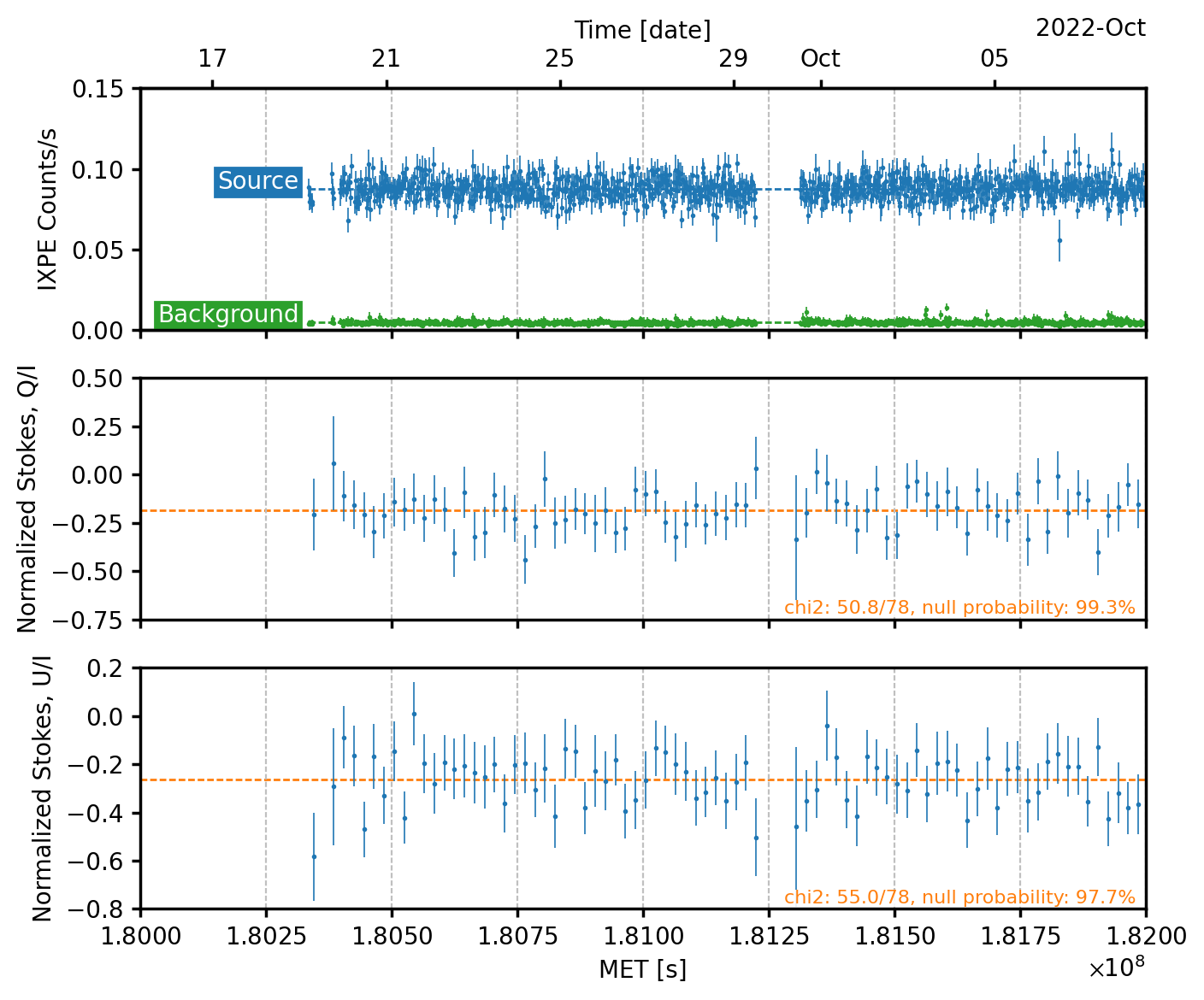
Figure 5: Top panel: 1RXS J1708 light curve, averaged over the three IXPE telescopes, for the source and the background. The count rate is averaged over 500 seconds and integrated over the IXPE nominal energy band, $2.0$–$8.0$  keV. Middle and bottom panels: light curve of normalized Stokes parameters; the time bin is 20 ks. In all panels variations are compatible with statistical fluctuations only: the null probabilty for a fit with a constant is acceptable.

A.2 NICER

In order to complement the IXPE  data, we requested a set of new NICER observations, which have been awarded and performed a week after the end of the last IXPE  observation. However, all these observations suffered from high optical loading (resulting from a low Sun angle), and thus were unusable for our analysis. We therefore resorted to the use of the NICER archival data, using the most recent available observations (closest in time to the IXPE  observation). Specifically, for the contemporaneous spectral fitting with IXPE and Swift spectra, we made use of the observations from 2022-08-21 (ObsID 5593051301).

The data were processed using version 9 of the NICER Data Analysis Software (NICERDAS) on version 6.30.1 of HEASoft. We applied standard filtering criteria as per the default cuts with nicerl2, resulting in 972 s of filtered exposure. The spectrum was then binned with optimal binning (Kaastra & Bleeker, 2016) and with a minimum of 25 counts per bin. The background spectrum was generated using version 7 of the 3C50 model (Remillard et al., 2022). The rmf and arf files were generated from nicerrmf and nicerarf, respectively.

A.3 Swift

A Swift-XRT target of opportunity observation was performed on 2022-10-20 for a total of 1020 s in Windowed Timing (WT) mode. The data were processed using the standard HEASoft tools, extracting the spectra using xselect, after generating ancillary response file using xrtmkarf and the latest calibration files available in the Swift-XRT CALDB. The source was extracted from the cleaned event file using a centered circular region with a radius of 17 pixels. The background region was extracted using an off-centered circular region of the same radius. The extracted source spectra were binned, requiring each spectral channel to have at least 25 counts.

Appendix B Model parameters from the spectro-polarimetric analysis

As discussed in § 3, there are two possible spectral decompositions that are both compatible with the data: one consists of a thermal (blackbody) component plus a non thermal (power law) and the second consists of two blackbodies. The best fitting model parameters, for the two cases, are listed in Table 2.

Model parameters	value	model parameters	value
DU1 normalization	1.0 (frozen)	DU1 normalization	1.0 (frozen)
TBabs nH [ 1022 cm-2]	2.085${}^{+0.055}_{-0.050}$	TBabs nH [ 1022 cm-2]	1.391${}^{+0.039}_{-0.038}$
kT${}_{\textrm{bbody}}$ [ keV ]	0.4546${}^{+0.0077}_{-0.0058}$	kT${}_{\textrm{bbody1}}$ [ keV ]	0.4354${}^{+0.0076}_{-0.0078}$
norm${}_{\textrm{bbody}}$	0.0002293${}^{+0.0000179}_{-0.0000096}$	norm${}_{\textrm{bbody1}}$	0.0005440${}^{+0.0000097}_{-0.0000091}$
PD${}_{\textrm{bbody}}$	1.0 (U.L.) ‡	PD${}_{\textrm{bbody1}}$	0.060${}^{+0.036}_{-0.037}$
PA${}_{\textrm{bbody}}$ [ deg ]	30.5${}^{+3.4}_{-3.3}$	PA${}_{\textrm{bbody1}}$ [ deg ]	$-69.0^{+16.7}_{-18.2}$
PowLaw Photon Index	2.9672${}^{+0.0092}_{-0.0567}$	kT${}_{\textrm{bbody2}}$ [ keV ]	1.073${}^{+0.031}_{-0.029}$
norm${}_{\textrm{PowLaw}}$	0.04101${}^{+0.00059}_{-0.00382}$	norm${}_{\textrm{bbody2}}$	0.0002324${}^{+0.0000082}_{-0.0000079}$
PD${}_{\textrm{power law}}$	0.768${}^{+0.041}_{-0.040}$	PD${}_{\textrm{bbody2}}$	0.728${}^{+0.038}_{-0.037}$
PA${}_{\textrm{power law}}$ [ deg ]	$-60.8^{+1.0}_{-1.2}$	PA${}_{\textrm{bbody2}}$ [ deg ]	$-61.0^{+1.4}_{-1.4}$
DU2 normalization	0.9567${}^{+0.0051}_{-0.0049}$	DU2 normalization	0.9568${}^{+0.0053}_{-0.0052}$
DU3 normalization	0.8921${}^{+0.0048}_{-0.0046}$	DU3 normalization	0.8922${}^{+0.0049}_{-0.0049}$
Swift/XRT normalization	0.922${}^{+0.032}_{-0.032}$	Swift/XRT normalization	0.934${}^{+0.032}_{-0.032}$
NICER normalization	1.062${}^{+0.013}_{-0.011}$	NICER normalization	1.075${}^{+0.013}_{-0.013}$
$\chi^{2}$	410.4 with 408 d.o.f.	$\chi^{2}$	405.8 with 408 d.o.f.
Null prob	45.7%	Null prob	52.2%

Table 2: Model parameters for the joint spectropolarimetric fit of IXPE  Swift/XRT and NICER data. Uncertainties are calculated at the 68.3% confidence level for one parameter of interest. The two leftmost columns refer to the model TBabs*(bbody * polconst + powerlaw * polconst). The normalization of the BB components is defined as $L_{39}/D_{10}^{2}$, where $L_{39}$ is the BB luminosity in units of $10^{39}$ erg/s and $D_{10}$ is the distance to the source in units of 10 kpc. The PL normalization is in units of counts keV^-1 cm^-2s^-1 at 1 keV. The rightmost two columns are for the model TBabs*(bbody * polconst + bbody * polconst).
^‡ In this case, the confidence level for the polarization degree of the BB component is not closed, and it was only possible to set an upper limit (U.L.). The value of this parameter is poorly constrained: by freezing the value of PD${}_{\textrm{bbody1}}$ to 0.2 also returns an acceptable fit (see the text for details).

Appendix C Timing Solution

A timing solution of the count rate data, has been obtained by following the procedure from Bachetti et al. (2022). We first determined an approximate solution and then used the Pletsch & Clark (2015) Maximum Likelihood method to refine it. We determined an approximate first solution with the tool HENzsearch, running a $Z^{2}_{3}$ search (Buccheri et al., 1983) around the known pulse frequency from Dib & Kaspi (2014). The pulsar was detected with extremely high significance, with $Z^{2}_{3}\sim 16000$ ($\sim$ 126$\sigma$, considering 10000 trials), at $f=0.09079575$ Hz and $\dot{f}=-2.28\times 10^{-13}$ Hz s^-1. Then, we used the tool ell1fit v. 0.2 to run a Maximum Likelihood fit of the spin solution, using a template for the pulse profile obtained by a Fourier analysis with 4 harmonics, and letting only the spin frequency and its first spin derivative vary. The resulting solution, using epoch MJD 59850.84175 (TDB) as a reference, is $f= 0.090795742(5)$ Hz, $\dot{f}=-1.87(25)\times 10^{-13}$ Hz s^-1. The addition of the second frequency derivative did not improve the fit significantly: the 3 $\sigma$ upper limit on the second derivative in our observation is $\sim 2\times 10^{-19}$ Hz s^-2.

References

- Anders & Grevesse (1989) Anders, E., & Grevesse, N. 1989, Geochim. Cosmochim. Acta, 53, 197, doi: 10.1016/0016-7037(89)90286-X
- Arnaud (1996) Arnaud, K. A. 1996, in Astronomical Society of the Pacific Conference Series, Vol. 101, Astronomical Data Analysis Software and Systems V, ed. G. H. Jacoby & J. Barnes, 17
- Arzoumanian et al. (2014) Arzoumanian, Z., Gendreau, K. C., Baker, C. L., et al. 2014, in Society of Photo-Optical Instrumentation Engineers (SPIE) Conference Series, Vol. 9144, Space Telescopes and Instrumentation 2014: Ultraviolet to Gamma Ray, ed. T. Takahashi, J.-W. A. den Herder, & M. Bautz, 914420, doi: 10.1117/12.2056811
- Bachetti et al. (2022) Bachetti, M., Heida, M., Maccarone, T., et al. 2022, ApJ, 937, 125, doi: 10.3847/1538-4357/ac8d67
- Baldini et al. (2022) Baldini, L., Bucciantini, N., Di Lalla, N., et al. 2022, SoftwareX, 19, 101194, doi: 10.1016/j.softx.2022.101194
- Buccheri et al. (1983) Buccheri, R., Bennett, K., Bignami, G. F., et al. 1983, A&A, 128, 245
- Burrows et al. (2005) Burrows, D. N., Hill, J. E., Nousek, J. A., et al. 2005, Space Sci. Rev., 120, 165, doi: 10.1007/s11214-005-5097-2
- Caiazzo et al. (2022) Caiazzo, I., González-Caniulef, D., Heyl, J., & Fernández, R. 2022, MNRAS, 514, 5024, doi: 10.1093/mnras/stac1571
- Coti Zelati et al. (2018) Coti Zelati, F., Rea, N., Pons, J. A., Campana, S., & Esposito, P. 2018, MNRAS, 474, 961, doi: 10.1093/mnras/stx2679
- Di Marco et al. (2023) Di Marco et al. 2023, in preparation
- Dib & Kaspi (2014) Dib, R., & Kaspi, V. M. 2014, ApJ, 784, 37, doi: 10.1088/0004-637X/784/1/37
- Duncan & Thompson (1992) Duncan, R. C., & Thompson, C. 1992, ApJ, 392, L9, doi: 10.1086/186413
- Durant & van Kerkwijk (2006) Durant, M., & van Kerkwijk, M. H. 2006, ApJ, 650, 1070, doi: 10.1086/506380
- González-Caniulef et al. (2022) González-Caniulef, D., Caiazzo, I., & Heyl, J. 2022, arXiv e-prints, arXiv:2204.00140. https://arxiv.org/abs/2204.00140
- González Caniulef et al. (2016) González Caniulef, D., Zane, S., Taverna, R., Turolla, R., & Wu, K. 2016, MNRAS, 459, 3585, doi: 10.1093/mnras/stw804
- González-Caniulef et al. (2019) González-Caniulef, D., Zane, S., Turolla, R., & Wu, K. 2019, MNRAS, 483, 599, doi: 10.1093/mnras/sty3159
- Götz et al. (2007) Götz, D., Rea, N., Israel, G. L., et al. 2007, A&A, 475, 317, doi: 10.1051/0004-6361:20078291
- Heyl & Shaviv (2000) Heyl, J. S., & Shaviv, N. J. 2000, MNRAS, 311, 555, doi: 10.1046/j.1365-8711.2000.03076.x
- Heyl & Shaviv (2002) —. 2002, Phys. Rev. D, 66, 023002, doi: 10.1103/PhysRevD.66.023002
- Ho & Lai (2003) Ho, W. C. G., & Lai, D. 2003, MNRAS, 338, 233, doi: 10.1046/j.1365-8711.2003.06047.x
- Israel et al. (1999) Israel, G. L., Covino, S., Stella, L., et al. 1999, ApJ, 518, L107, doi: 10.1086/312077
- Joye & Mandel (2003) Joye, W. A., & Mandel, E. 2003, in Astronomical Society of the Pacific Conference Series, Vol. 295, Astronomical Data Analysis Software and Systems XII, ed. H. E. Payne, R. I. Jedrzejewski, & R. N. Hook, 489
- Kaastra & Bleeker (2016) Kaastra, J. S., & Bleeker, J. A. M. 2016, A&A, 587, A151, doi: 10.1051/0004-6361/201527395
- Kaspi & Beloborodov (2017) Kaspi, V. M., & Beloborodov, A. M. 2017, ARA&A, 55, 261, doi: 10.1146/annurev-astro-081915-023329
- Kislat et al. (2015) Kislat, F., Clark, B., Beilicke, M., & Krawczynski, H. 2015, Astroparticle Physics, 68, 45, doi: 10.1016/j.astropartphys.2015.02.007
- Krawczynski et al. (2022) Krawczynski, H., Taverna, R., Turolla, R., Mereghetti, S., & Rigoselli, M. 2022, A&A, 658, A161, doi: 10.1051/0004-6361/202142085
- Kuiper et al. (2006) Kuiper, L., Hermsen, W., den Hartog, P. R., & Collmar, W. 2006, ApJ, 645, 556, doi: 10.1086/504317
- Lloyd (2003) Lloyd, D. A. 2003, arXiv e-prints, astro. https://arxiv.org/abs/astro-ph/0303561
- Medin & Lai (2007) Medin, Z., & Lai, D. 2007, MNRAS, 382, 1833, doi: 10.1111/j.1365-2966.2007.12492.x
- Mori & Ho (2007) Mori, K., & Ho, W. C. G. 2007, MNRAS, 377, 905, doi: 10.1111/j.1365-2966.2007.11663.x
- Perna et al. (2001) Perna, R., Heyl, J. S., Hernquist, L. E., Juett, A. M., & Chakrabarty, D. 2001, ApJ, 557, 18, doi: 10.1086/321569
- Pletsch & Clark (2015) Pletsch, H. J., & Clark, C. J. 2015, ApJ, 807, 18, doi: 10.1088/0004-637X/807/1/18
- Potekhin et al. (2012) Potekhin, A. Y., Suleimanov, V. F., van Adelsberg, M., & Werner, K. 2012, A&A, 546, A121, doi: 10.1051/0004-6361/201219747
- Rea & Esposito (2011) Rea, N., & Esposito, P. 2011, in Astrophysics and Space Science Proceedings, Vol. 21, High-Energy Emission from Pulsars and their Systems, 247, doi: 10.1007/978-3-642-17251-9_21
- Rea et al. (2003) Rea, N., Israel, G. L., Stella, L., et al. 2003, ApJ, 586, L65, doi: 10.1086/374585
- Rea et al. (2007) Rea, N., Israel, G. L., Oosterbroek, T., et al. 2007, Ap&SS, 308, 505, doi: 10.1007/s10509-007-9310-5
- Remillard et al. (2022) Remillard, R. A., Loewenstein, M., Steiner, J. F., et al. 2022, AJ, 163, 130, doi: 10.3847/1538-3881/ac4ae6
- Strohmayer (2017) Strohmayer, T. E. 2017, ApJ, 838, 72, doi: 10.3847/1538-4357/aa643d
- Sugizaki et al. (1997) Sugizaki, M., Nagase, F., Torii, K., et al. 1997, PASJ, 49, L25, doi: 10.1093/pasj/49.5.L25
- Taverna et al. (2015) Taverna, R., Turolla, R., Gonzalez Caniulef, D., et al. 2015, MNRAS, 454, 3254, doi: 10.1093/mnras/stv2168
- Taverna et al. (2020) Taverna, R., Turolla, R., Suleimanov, V., Potekhin, A. Y., & Zane, S. 2020, MNRAS, 492, 5057, doi: 10.1093/mnras/staa204
- Taverna et al. (2022) Taverna, R., Turolla, R., Muleri, F., et al. 2022, Science, 378, 646, doi: 10.1126/science.add0080
- Thompson & Duncan (1993) Thompson, C., & Duncan, R. C. 1993, ApJ, 408, 194, doi: 10.1086/172580
- Turolla et al. (2015) Turolla, R., Zane, S., & Watts, A. L. 2015, Reports on Progress in Physics, 78, 116901, doi: 10.1088/0034-4885/78/11/116901
- van Adelsberg & Perna (2009) van Adelsberg, M., & Perna, R. 2009, MNRAS, 399, 1523, doi: 10.1111/j.1365-2966.2009.15374.x
- Voges et al. (1999) Voges, W., Aschenbach, B., Boller, T., et al. 1999, A&A, 349, 389. https://arxiv.org/abs/astro-ph/9909315
- Weisskopf et al. (2022) Weisskopf, M. C., Soffitta, P., Baldini, L., et al. 2022, Journal of Astronomical Telescopes, Instruments, and Systems, 8, 1 , doi: 10.1117/1.JATIS.8.2.026002
- Wilms et al. (2000) Wilms, J., Allen, A., & McCray, R. 2000, ApJ, 542, 914, doi: 10.1086/317016
- Xie et al. (2022) Xie, F., Di Marco, A., La Monaca, F., et al. 2022, Nature, 612, 658, doi: 10.1038/s41586-022-05476-5
- Zane & Turolla (2006) Zane, S., & Turolla, R. 2006, MNRAS, 366, 727, doi: 10.1111/j.1365-2966.2005.09784.x