[O III] 5007Å Emission Line Width as a Surrogate for $\sigma_{*}$ in Type 1 AGNs?

Abstract

We present a study of the relation between the [O III] 5007Å emission line width ($\rm\sigma_{[OIII]}$) and stellar velocity dispersion ($\sigma_{*}$), utilizing a sample of 740 type 1 active galactic nuclei (AGNs) with high-quality spectra at redshift z $<$ 1.0. We find the broad correlation between the core component of [O III] emission line width ($\rm\sigma_{[OIII,core]}$) and $\sigma_{*}$ with a scatter of 0.11 dex for the low redshift (z $<$ 0.1) sample; for redshift (0.3 $<$ z $<$ 1.0) AGNs, the scatter is larger, being 0.16 dex. We also find that the Eddington ratio ($\rm L_{bol}/L_{Edd}$) may play an important role in the discrepancies between $\rm\sigma_{[OIII,core]}$ and $\sigma_{*}$. As the $\rm L_{bol}/L_{Edd}$ increases, $\rm\sigma_{[OIII,core]}$ tends to be larger than $\sigma_{*}$. By classifying our local sample with different minor-to-major axis ratios, we find that $\sigma_{*}$ is larger than $\rm\sigma_{[OIII,core]}$ for those edge-on spiral galaxies. In addition, we also find that the effects of outflow strength properties such as maximum outflow velocity ($\rm V_{max}$) and the broader component of [O III] emission line width and line shift ($\rm\sigma_{[OIII,out]}$ and $\rm V_{[OIII,out]}$) may play a major role in the discrepancies between $\rm\sigma_{[OIII,core]}$ and $\sigma_{*}$. The discrepancies between $\rm\sigma_{[OIII,core]}$ and $\sigma_{*}$ are larger when $\rm V_{max}$, $\rm V_{[OIII,out]}$, and $\rm\sigma_{[OIII,out]}$ increase. Our results show that the outflow strengths may have significant effects on the differences between narrow-line region gas and stellar kinematics in AGNs. We suggest that caution should be taken when using $\rm\sigma_{[OIII,core]}$ as a surrogate for $\sigma_{*}$. In addition, the substitute of $\rm\sigma_{[OIII,core]}$ for $\sigma_{*}$ could be used only for low luminosity AGNs.

1. INTRODUCTION

Black-hole mass (M_BH) is a fundamental driving factor in active galactic nuclei (AGNs). The study of the correlations between M_BH and properties of their host galaxies is important in understanding the physical nature and the growth history of AGNs. Over the last two decades, there have been many studies for investigating the co-evolution between supermassive black holes and their host galaxies (e.g., Ferrarese & Merrit, 2000; Gebhardt et al., 2000; McLure & Jarvis, 2002; Tremaine et al., 2002; Woo et al., 2006, 2010; Xue et al., 2010; Kormendy & Ho, 2013; Le et al., 2014; Sun et al., 2015; Shankar et al., 2016; Xue, 2017; Shankar et al., 2019; Le & Woo, 2019; Woo et al., 2019; Lin et al., 2022; Ayubinia et al., 2022). The tight correlations between M_BH and their host galaxies suggest that black holes and their hosts are co-evolving and regulating each other. These scaling relations could be explained by either mutual merger processes or AGN feedback (Silk & Rees, 1998; Peng et al., 2006).

In spite of the tight correlations between black holes and their host galaxies, it is difficult for us to measure the host galaxy properties due to AGNs often outshining their host galaxies. In particular, the measurement of stellar velocity dispersions ($\sigma_{*}$) is challenging because of the contamination of AGN continuum and emission lines in the observed spectra (particularly for high redshift AGNs). To overcome this issue, some studies have suggested using the line width of [O III] 5007Å ($\rm\sigma_{[OIII]}$) as a surrogate for the stellar velocity dispersion ($\sigma_{*}$) by assuming that the ionized gas kinematics of the narrow-line region (NLR) is followed the gravitational potential of the bulge of the host galaxy (e.g., Wilson & Heckman, 1985; Terlevich, Diaz & Terlevich, 1990; Whittle, 1992; Nelson & Whittle, 1996; Nelson, 2000; Boroson, 2003; Shields et al., 2003; Greene & Ho, 2005; Rice et al., 2006; Netzer & Trakhtenbrot, 2007; Salviander et al., 2007; Salviander & Shields, 2013). By analyzing in detail the [O III] kinematics, Wilson & Heckman (1985) is the first study which found that $\rm\sigma_{[OIII]}$ is correlated well with $\sigma_{*}$. Later on, using a large sample of 75 Seyfert galaxies, Nelson & Whittle (1996) found that there is a strong correlation between $\sigma_{*}$ and [O III] profile. By using 21 radio-quiet quasars, Bonning et al. (2005) found that $\rm\sigma_{[OIII]}$ is on average consistent with $\sigma_{*}$, converted from the Faber-Jackson relation. Using a large sample from the Sloan Digital Sky Survey (SDSS, York et al., 2000), Salviander, Shields & Bonning (2015) found a similar result as that of Bonning et al. (2005), supporting for the use of $\rm\sigma_{[OIII]}$ as a surrogate for $\sigma_{*}$ in statistical studies.

The use of $\rm\sigma_{[OIII]}$ to replace for $\sigma_{*}$ is appealing because it is easy for us to detect and measure $\rm\sigma_{[OIII]}$ for low and high redshift AGNs. Thus, the [O III] emission line plays an important role in the study of cosmic evolution between M_BH and their host galaxies. However, some studies have also found that the [O III] emission line often shows an asymmetric profile (e.g., the blue wing component) which could be interpreted as signatures of the non-gravitational potential such as outflows (e.g., Heckman et al., 1984; Bae & Woo, 2014; Woo et al., 2016; Le et al., 2017). Because of this reason, some studies have suggested using only the core component of [O III] emission line ($\rm\sigma_{[OIII,core]}$) as a surrogate for $\sigma_{*}$ (e.g., Greene & Ho, 2005; Komossa & Xu, 2007; Bennert et al., 2018). Greene & Ho (2005) found that after correcting for the blue wing component in the [O III] profile, $\sigma_{*}$ is traced well by $\rm\sigma_{[OIII]}$, albeit with large scatter. In addition, some other studies also proposed to use other NLR emission lines which have lower ionization potential compared to that of [O III], suffering less from outflow effects, such as [O II] 3727Å, [N II] 6583Å and [S II] 6716Å,3731Å (e.g., Phillips et al., 1986; Greene & Ho, 2005; Komossa & Xu, 2007; Ho, 2009; Bennert et al., 2018). However, the use of those emission lines as a surrogate for $\sigma_{*}$ also shows large scatter as the case of using $\rm\sigma_{[OIII,core]}$. Although the correlation between $\rm\sigma_{[OIII,core]}$ and $\sigma_{*}$ has been investigated by many studies, the driving factor for the large scatter between both components is still unclear.

Most of the studies of comparison between $\rm\sigma_{[OIII]}$ and $\sigma_{*}$ are carried out by indirect comparison between the M_BH$-$$\rm\sigma_{[OIII]}$ and M_BH$-$$\rm\sigma_{*}$ relations (e.g., Nelson, 2000; Boroson, 2003; Komossa & Xu, 2007; Grupe & Mathur, 2004; Wang & Lu, 2001). Until now, there are a few studies in which the authors directly and simultaneously compare $\rm\sigma_{[OIII]}$ and $\sigma_{*}$. Using 1749 type 2 Seyfert galaxies, Greene & Ho (2005) studied the direct comparison between $\rm\sigma_{[OIII]}$ and $\sigma_{*}$. They found that $\rm\sigma_{[OIII,core]}$ is consistent with $\sigma_{*}$ after removing for the asymmetric blue wing in the [O III] profile, and the ratio $\rm\sigma_{[OIII]}$$/$$\sigma_{*}$ is larger as the Eddington ratio increases. Rice et al. (2006) analyzed 24 low redshift targets of mostly type 2 AGNs using spatially resolved spectra of Hubble Space Telescope and found that the scatter between $\rm\sigma_{[OIII]}$ and $\sigma_{*}$ is complicated and cannot be corrected by using a simple relation. Ho (2009) did a similar study as that of Greene & Ho (2005) but for the [N II] 6583Å emission line by using 345 galaxies from the Palomar spectroscopy survey, and found consistent results as those of Greene & Ho (2005). For a larger sample, Woo et al. (2016) used 39,000 type 2 AGNs at z $<$ 0.3 to compare directly $\rm\sigma_{[OIII]}$ and $\sigma_{*}$. They found that $\rm\sigma_{[OIII]}$ fitted with double Gaussian is larger than $\sigma_{*}$ by a factor of 1.3-1.4, suggesting that the non-gravitational component (e.g., outflows) is relatively comparable to the gravitational potential. Recently, by using the SDSS sample of 611 hidden type 1 AGNs, Eun, Woo & Bae (2017) investigated that $\sigma_{*}$ is consistent with velocity dispersions of [N II] and $\rm\sigma_{[OIII,core]}$. Bennert et al. (2018) used 59 long-slit, high signal-to-noise (S/N) and spatially resolved Keck spectra to have a direct comparison of the relationship between $\rm\sigma_{[OIII,core]}$ and $\sigma_{*}$. They found large scatter in the correlation between $\rm\sigma_{[OIII,core]}$ and $\sigma_{*}$ in their sample and suggested that the use of $\rm\sigma_{[OIII,core]}$ as a surrogate for $\sigma_{*}$ should take caution when applied for individual targets.

Besides the studies of comparison between $\rm\sigma_{[OIII]}$ and $\sigma_{*}$, studying the velocity offset of [O III] emission line ($\rm V_{[OIII]}$) is an interesting topic for exploring AGN-driven outflows. Many works have investigated $\rm V_{[OIII]}$ with respect to the systemic velocity of the host galaxy or lower ionization lines such as [O II] or [S II] (e.g., Crenshaw & Kraemer, 2000; Zamanov et al., 2002; Eracleous & Halpern, 2004; Boroson, 2005; Hu et al., 2008; Komossa et al., 2008; Zhang et al., 2011; Bae & Woo, 2014). Using high-quality spatially resolved spectra, Crenshaw & Kraemer (2000) studied the acceleration radial velocity based on the peak of [O III] emission line and interpreted their results using the AGN-driven biconical radial outflow model. Using single-aperture spectra, the velocity offset of the peak of [O III] has been investigated statistically (Zamanov et al., 2002; Eracleous & Halpern, 2004; Boroson, 2005; Hu et al., 2008). Boroson (2005) found that more than half of their sources show blueshifted of the [O III] peaks with respect to the systemic velocity based on other lower ionization lines. They suggested that the blueshifted $\rm V_{[OIII]}$ may be governed by AGN-properties such as M_BH and Eddington ratio. Interestingly, the blueshifts of higher ionization lines such as [O III] are larger compared to that of lower ionization lines, e.g., [O II], [S II], [N II] (Eracleous & Halpern, 2004; Boroson, 2005; Hu et al., 2008). By using a small sample of narrow-line Seyfert 1 galaxies with strong blueshifted [O III], Komossa et al. (2008) found that the velocity shift of the core component of [O III] emission line ($\rm V_{[OIII,core]}$) shows a moderate correlation with Eddington ratio and optical Fe II strength. Zhang et al. (2011) found similar results but a weak correlation between $\rm V_{[OIII,core]}$ and Eddington ratio by using homogenous samples of radio-quiet Seyfert 1 galaxies. Using a large sample, $\sim$23,000 type 2 AGNs, Bae & Woo (2014) found that half of their sources show $\rm V_{[OIII]}$ ¿ 20 km s^-1, and the fractions of such $\rm V_{[OIII]}$ in type 1 and type 2 AGNs are similar after considering orientation effects. In short, the velocity of [O III] emission line does show some offset with respect to the systemic velocity. Particularly, the core component of [O III] also shows some offset and has weak or moderate correlations with AGN properties (e.g., Eddington ratio). It is therefore important that we should consider analyzing $\rm V_{[OIII]}$ when studying the correlation between $\rm\sigma_{[OIII,core]}$ and $\sigma_{*}$. $\rm V_{[OIII]}$ with respect to the systemic velocity may have impacts on the discrepancies between $\rm\sigma_{[OIII,core]}$ and $\sigma_{*}$.

In general, the correlations between $\rm\sigma_{[OIII,core]}$ and $\sigma_{*}$ mean that they are tracing the same velocity field of the gravitational potential. However, there is large scatter in these correlations and the driving factors for these discrepancies are still unclear. Therefore, a detailed study using a high S/N spectral sample is necessary for robust measurements of both $\rm\sigma_{[OIII]}$ and $\sigma_{*}$, and crucial for understanding the physically driven properties of gas and stellar kinematics in type 1 AGNs. In particular, for high redshift AGNs, we often utilize $\rm\sigma_{[OIII]}$ as a surrogate for $\sigma_{*}$ since it is challenging to measure $\sigma_{*}$ for high redshift objects. It is necessary to have a proper study for the relations between $\rm\sigma_{[OIII]}$ and $\sigma_{*}$ for high redshift AGNs.

In this paper, we present a detailed comparison between $\rm\sigma_{[OIII]}$ and $\sigma_{*}$ for not only local AGNs but also for high redshift AGNs. For local AGNs (z $<$ 0.1), the sample from Bennert et al. (2018) with long-slit and high-quality spatially resolved $\sigma_{*}$ is a suitable sample for studying the relation between $\rm\sigma_{[OIII]}$ and $\sigma_{*}$ that has robust measurements of both quantities. In this study, by using the 59 local AGNs from Bennert et al. (2018), we investigate in detail the discrepancy between $\rm\sigma_{[OIII]}$ and $\sigma_{*}$ as a function of AGN properties. Then, we apply the same approach for studying the local sample which has integrated spectra, observed with a larger aperture size (3$\arcsec$) by SDSS, including 611 hidden type 1 AGNs from Eun, Woo & Bae (2017). For high redshift AGNs (0.3 $<$ z $<$ 1.0), we select 18 high S/N Keck spectra (Woo et al., 2006, 2008) and 52 co-added high S/N spectra from the SDSS Reverberation Mapping (SDSS-RM) project (Shen et al., 2015). Finally, our sample includes 740 targets at redshift z $<$ 1.0, covering the broad dynamic ranges of $\mathrm{\lambda L_{5100}\sim 10^{41.5}-10^{46.0}}$ erg s^-1and 6.5 $<$ $\log($M_BH) $<$ 9.5. The high-quality spectra of this sample enable robust measurements of $\rm\sigma_{[OIII]}$ and $\sigma_{*}$, hence providing us a good opportunity for studying in detail the direct relationship between both components and investigating for the physically driving factors of the discrepancies between them.

In Section 2, we describe the sample selection. Sections 3 and 4 present the measurements and results, respectively. The discussions and summary are presented in Sections 5 and 6, respectively. The following cosmological parameters are used throughout the paper: $H_{0}=70$ km s^-1 Mpc^-1, $\Omega_{\rm m}=0.30$, and $\Omega_{\Lambda}=0.70$.

2. Sample Selection

In this work, we combined the aforementioned low and high redshift samples (z $<$ 1.0) which allow for robust measurements of $\sigma_{*}$ and the [O III] emission line widths ($\rm\sigma_{[OIII,core]}$ and $\rm\sigma_{[OIII,broad]}$) to have a detailed study on the correlations between gas and stellar kinematics not only for local AGNs but also for high redshift ones.

Firstly, for the local AGN sample (z $<$ 0.1), we selected 59 targets of Bennert et al. (2018) which have observed using Low Resolution Imaging Spectrometer (LRIS, Oke et al., 1995) at the Keck telescope. Those targets have high S/N spectra which provide robust measurements of spatially resolved $\sigma_{*}$ within the bulge radius (Harris et al., 2012). In addition, for studying the relation between $\sigma_{*}$ and $\rm\sigma_{[OIII,core]}$ measured from the integrated SDSS spectra (aperture size 3$\arcsec$), we utilized 611 hidden type 1 AGNs (hereafter, local SDSS sample) from Eun, Woo & Bae (2017) which have reliable measurements of $\sigma_{*}$ and $\rm\sigma_{[OIII,core]}$.

Secondly, for high redshift AGNs (0.3 $<$ z $<$ 1.0), we chose 18 sources from Woo et al. (2006, 2008). The sample was also observed using LRIS-Keck, and has high S/N spectra which allowed for subtracting the contamination of AGN continuum component in the stellar feature, leading to reliable estimation of $\sigma_{*}$. To enlarge the dynamic range of AGN luminosity, we selected 88 co-added sources with co-added high S/N spectra from the SDSS-RM project (Shen et al., 2015) which have robust measurements of $\sigma_{*}$. Among them, we removed 36 sources which have large noisy distortion surrounding the [O III] and H$\beta$ emission line profiles. Then, the remaining SDSS-RM sample has 52 sources which have reliable determinations of both $\sigma_{*}$ and $\rm\sigma_{[OIII]}$. In total, we obtained 70 AGNs (hereafter, high redshift sample) which have a unique broad luminosity dynamic range and are suitable for studying the relation between $\sigma_{*}$ and $\rm\sigma_{[OIII,core]}$ at redshift 0.3 $<$ z $<$ 1.0. With the advantages of high-quality spectral sample observed with LRIS-Keck and co-added high S/N SDSS-RM spectra, we carry out a detailed study of the direct relation between $\sigma_{*}$ and $\rm\sigma_{[OIII,core]}$ for high redshift AGNs.

Finally, our sample included 740 local and high redshift AGNs, covering the broad dynamic ranges of $\mathrm{\lambda L_{5100}\sim 10^{41.5}-10^{46.0}}$ erg s^-1 and 6.5 $<$ $\log($M_BH) $<$ 9.5 (see Section 3.1). Figure 1 shows the distributions of $\mathrm{M_{\rm BH}}$ and continuum luminosity $\mathrm{L_{5100}}$ of our sample.

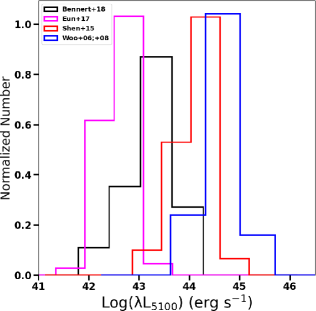
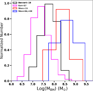
Figure 1.— Distributions of continuum luminosity at 5100 Å (left panel) and black-hole mass (right panel). The magenta, black, blue, and red histograms show the distributions of the samples of Eun, Woo & Bae (2017), Bennert et al. (2018), Woo et al. (2006, 2008), and Shen et al. (2015), respectively.

3. Measurements

3.1. Spectral Analysis and AGN property measurements

In our study, we have four different subsamples of Woo et al. (2006, 2008), Shen et al. (2015), Eun, Woo & Bae (2017) and Bennert et al. (2018). In this section, we describe the spectral analysis processes of those subsamples to obtain pure emission spectra for measuring AGN properties.

Similar to 18 targets of Woo et al. (2006, 2008), 59 AGNs from Bennert et al. (2018) were also observed with LRIS-Keck. So, the data reduction and spectral analysis of both samples were similar to each other. In our previous work in Woo et al. (2018), we have updated the multi-component spectral analysis of 18 sources in Woo et al. (2006, 2008) following the proredure of Park et al. (2015). Similarly, Bennert et al. (2018) also applied the method of Park et al. (2015) in their spectral analysis. Here, we briefly describe the recipe of our optical spectral analysis. A model with a combination of the pseudo-continuum including a single power law and an Fe II component based on the I Zw 1 Fe II template (Boroson & Green, 1992), as well as a host-galaxy component adopted from the stellar template of the Indo-US spectral library in Valdes et al. (2004) was applied to fit the observed optical spectra within the wavelength ranges of 4430Å $-$ 4770Å and 5080Å $-$ 5450Å. The best-fit model was determined using the $\chi^{2}$ minimization from MPFIT. After subtracting the pseudo-continuum from the observed spectra, a sixth order Gauss-Hermite series was applied to fit the broad component of the H$\beta$ emission line. The narrow component of H$\beta$ was modeled separately by using the [O III] 5007Å best-fit model. From the best-fit model, we measured line width ($\rm FWHM_{H\beta}$), line dispersion ($\rm\sigma_{H\beta}$), the luminosity of the H$\beta$ line ($\rm L_{H\beta}$), and the monochromatic luminosity at 5100Å ($\rm L_{5100}$). The updated measured properties of 18 targets in Woo et al. (2006, 2008) can be found in Table 1 of Woo et al. (2018), and the resulting measurements of 59 sources of Bennert et al. (2018) are shown in Table 1 of Bennert et al. (2015).

For 52 sources from Shen et al. (2015), the authors have provided the co-added integrated spectra in their public catalog. To obtain the pure emission line spectra from the provided co-added spectra, we performed multi-component spectral analysis for 52 SDSS-RM spectra similarly as that for targets observed with LRIS-Keck. Figure 2 shows an example of multi-component fitting results for a target from the SDSS-RM sample.

The spectral analysis of the local SDSS sample is presented in detail in Section 2 of Eun, Woo & Bae (2017). This sample is basically selected from the type 2 AGN catalog of Bae & Woo (2014). After subtracting the SDSS spectra from the best-fit stellar population model using the penalized pixel-fitting code (pPXF, Cappellari & Emsellem, 2004), the authors identified the hidden type 1 AGNs among the type 2 AGNs based on a careful analysis of the broad component of H$\alpha$ emission line.

To have a consistent measurement of M_BH for all sources in our sample, we applied the single-epoch method, using the virial theorem and H$\beta$ size-luminosity relation based on the result of Bentz et al. (2013) (see equation 1 in Le, Woo & Xue, 2020) for calculating M_BH for the high redshift sample (Woo et al., 2006, 2008 and Shen et al., 2015). As in our previous work, we chose $\rm\sigma_{H\beta}$ and the monochromatic luminosity at 5100Å ($\rm L_{5100}$) for determining $\rm M_{BH}$ (Le, Woo & Xue, 2020). We used the virial factor (f = 4.47) from Woo et al. (2015) for the masses based on $\rm\sigma_{H\beta}$. From M_BH measurements, we determined Eddington ratio for our sample. The bolometric luminosity is calculated from the monochromatic luminosity at 5100Å ($\rm L_{bol}$ = 10$\times$$\rm L_{5100}$). For M_BH measurements of the local SDSS sample, Eun, Woo & Bae (2017) used the single-epoch method to determine M_BH for their sample using H$\beta$ and H$\alpha$ emission lines. We simply adopted their measurements in our analysis. Figure 3 displays the distributions of M_BH, $\rm L_{bol}$, and Eddington ratio for all subsamples of Bennert et al. (2018), Eun, Woo & Bae (2017), Woo et al. (2006, 2008) and Shen et al. (2015), respectively.

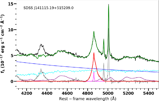
Figure 2.— Example of multi-component fitting result for the SDSS spectrum, SDSS J141115.19$-$515209.0 from the sample of Shen et al. (2015). The rest-frame SDSS spectrum is in thick black. The total model (green) includes power-law continuum (blue), Fe II model (purple), and stellar model (cyan). The continuum subtracted emission line is displayed in gray and the H$\beta$ line broad and narrow models are presented in red and pink, respectively.

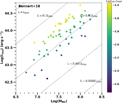
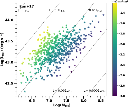
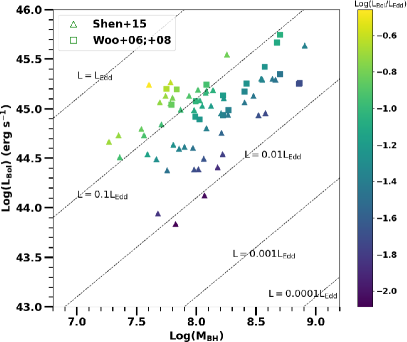
Figure 3.— Distributions of M_BH, $\rm L_{bol}$, and Eddington ratio for those subsamples of Bennert et al. (2018), Eun, Woo & Bae (2017), Woo et al. (2006, 2008) and Shen et al. (2015), repsectively. The dash lines indicate different Eddington ratios.

3.2. Stellar Velocity Dispersion and Velocity Shift

With the high S/N spectra of our selected sample, $\sigma_{*}$ has been robustly measured by previous works of Woo et al. (2006, 2008), Shen et al. (2015), Eun, Woo & Bae (2017), and Bennert et al. (2018). Basically, the authors used similar approaches for estimating $\sigma_{*}$ by comparing in the pixel space between the observed spectra and the Gaussian-broadened stellar template spectra (G and K giants). Therefore, in this work, we simply adopted those measurements for our analysis. Here, we briefly explain their measurements.

Woo et al. (2006, 2008) measured $\sigma_{*}$ for their sample by using stellar absorption lines around Mg b (5175Å) and Fe (5270Å). After subtracting the AGN Fe emission, the authors compared in the pixel space the pure observed spectra with five Gaussian-broadened stellar template spectra (G8, G9, K0, K2, and K5 giants). Then the final $\sigma_{*}$ estimations were based on the best-fit template.

For SDSS-RM targets, Shen et al. (2015) used the vdispfit package and the direct-pixel-fitting code Penalized Pixel-Fitting (pPXF) to measure $\sigma_{*}$. The measurement was obtained within the wavelength range of 4125-5350 Å containing the G band (4304Å), Mg Ib (5167Å, 5173Å, 5184Å), and Fe (5270Å). Given the advantage of high S/N co-added spectra, the authors obtained robust measurements for 88 targets among the total of 212 AGNs used in their sample. We neglected some sources which have noisy distortion surrounding the H$\beta$ and [O III] emission lines for a reliable comparison with $\sigma_{*}$. Finally, we selected 52 targets from Shen et al. (2015) in our study.

Similar to Woo et al. (2006, 2008), Bennert et al. (2018) compared their observed spectra with the Gaussian-broadened stellar templates of G, K, A0, and F2 stars from the Indo-US survey within three spectral regions of Ca H and Ca K (3969Å and 3934Å), Mg Ib (5167Å, 5173Å, 5184Å) and Ca II (8498Å, 8542Å, 8662Å). From the high-quality long-slit spectra of LRIS-Keck, the sample of Bennert et al. (2018) allowed for the robust measurements of spatially resolved $\sigma_{*}$ within the bulge radius (obtained from the surface photometry fitting of SDSS image, Harris et al., 2012).

Finally, for the local SDSS hidden type 1 AGN sample, Eun, Woo & Bae (2017) used $\sigma_{*}$ available from the MPA-JHU (Abazajian et al., 2009) catalog. We adopted those $\sigma_{*}$ values in our analysis.

All of the $\sigma_{*}$ used in this work were corrected for the instrumental resolution of LRIS-Keck ($\sim$58 km s^-1) and SDSS ($\sim$65 km s^-1), respectively.

The high S/N spectra of our selected samples also allow us to measure the stellar absorption line velocity ($\rm V_{*}$) accurately and provide a reliable systemic velocity for analyzing the kinematics of [O III] emission line. Therefore, we adopted $\rm V_{*}$ as systemic velocity in this work. We used the provided $\rm V_{*}$ from Woo et al. (2006, 2008), Shen et al. (2016), and Eun, Woo & Bae (2017). For 59 targets of Bennert et al. (2018), since the authors did not provide $\rm V_{*}$, we adopted the measured $\rm V_{*}$ of this sample (high S/N spectra, 38 sources) from Sexton et al. (2020) using the SDSS spectra. Sexton et al. (2020) developed the Bayesian decomposition analysis for SDSS spectra (BADASS) using Python. BADASS is a powerful fitting package for obtaining all spectral components of SDSS spectra simultaneously and accurately by utilizing a Markov-Chain Monte Carlo (MCMC) fitting technique.

3.3. Gas Emission Line Kinematics

In this section, we present the fitting model to measure $\rm\sigma_{[OIII]}$ and $\rm V_{[OIII]}$. In addition, we also measure outflow strength properties, e.g., maximum outflow velocity ($\rm V_{max}$), to study the effects of outflow strength on the relations between $\rm\sigma_{[OIII]}$ and $\sigma_{*}$ .

3.3.1 Line Width and Line Shift Measurements

Following the results of Bennert et al. (2018), a double Gaussian is the best approach to fit the [O III] emission line. In this fitting, a Gaussian is fitted to the narrow (core) component of the [O III] line ($\rm\sigma_{[OIII,core]}$). While, another Gaussian is modeled for the broader (outflow) component of the [O III] profile ($\rm\sigma_{[OIII,out]}$). Based on the best-fit model of the [O III] emission line, we calculated the second moment ($\rm\sigma_{[OIII]}$) as follows:

$$\sigma_{\rm[OIII]}^{2}=\frac{\int\lambda^{2}f_{\lambda}d\lambda}{\int f_{\lambda}d\lambda}-\lambda_{0}^{2},$$ (1)

Here, $f_{\lambda}$ is the flux at each wavelength. $\rm\lambda_{0}$ is the first moment (centroid wavelength) of the emission line which is calculated as follows:

$$\lambda_{0}=\frac{\int\lambda f_{\lambda}d\lambda}{\int f_{\lambda}d\lambda},$$ (2)

In our analysis, after subtracting the pseudo-continuum from the observed spectra, we also applied a double Gaussian to model the [O III] emission line for 18 targets of Woo et al. (2006, 2008) and 52 targets of Shen et al. (2015). However, in some targets, if the peak of the broader component model of the [O III] emission line is lower than the noise level in the continuum (i.e., the amplitude peak-to-noise ratio ¡ 3), we discarded the broad component as noise and used a single Gaussian function to fit the [O III] profile. Figure 4 presents examples of [O III] fitting models of S06 and SDSS J141324.28$+$530527.0 from the samples of Woo et al. (2006, 2008) and Shen et al. (2015), respectively. The measured [O III] dispersions $\rm\sigma_{[OIII,core]}$ and $\rm\sigma_{[OIII,out]}$ were also corrected for the instrumental resolution of LRIS-Keck ($\sim$58 km s^-1) and SDSS ($\sim$65 km s^-1), respectively.

As mentioned in Section 3.2, we adopted $\rm V_{*}$ as the systemic velocity. We measured the velocity shifts based on the peaks of the core ($\rm V_{[OIII,core]}$) and the broad ($\rm V_{[OIII,out]}$) components of [O III] emission line.

Similar to our analysis, Eun, Woo & Bae (2017) used a double Gaussian to model the [O III] emission line for the local SDSS sample. Section 3.1 of Eun, Woo & Bae (2017) presents their emission line fitting model in detail. We adopted the measurements in their provided catalog in our study.

For the 59 targets of Bennert et al. (2018), since the authors did not release the spectra, we simply adopted their measurements of $\rm\sigma_{[OIII,core]}$ (see Table 1 in Bennert et al., 2018). In addition, we also used the measured [O II] dispersion from Bennert et al. (2018) for further analysis in Section 4. For the velocity shift measurements, we adopted the measured $\rm V_{[OIII,core]}$ and $\rm V_{[OIII,out]}$ with respect to the stellar systemic velocity of this sample from Sexton et al. (2020) using the SDSS spectra. Among the 59 targets of Bennert et al. (2018), Sexton et al. (2020) measured $\rm V_{[OIII,core]}$ and $\rm V_{[OIII,out]}$ for 38 targets which show strong outflow signatures in their [O III] emission line profiles.

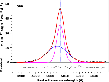
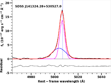
Figure 4.— Examples of [O III] 5007Å fitting models for S06 and SDSS J141324.28$+$530527.0 from the samples of Woo et al. (2006, 2008) and Shen et al. (2015), respectively. The total model is shown in red. The core component of [O III] is fitted by a Gaussian model and displayed in pink. The broader component (blue) is also fitted by a Gaussian function. The dash-line shows the rest-frame position of [O III] at 5007Å.

3.3.2 Maximum Outflow Velocity

$\rm\sigma_{[OIII,out]}$ is often considered as a tracer of outflow signatures in AGNs (e.g., Greene & Ho, 2005, Bae & Woo, 2014, Woo et al., 2016, Le et al., 2017). In our analysis, we determined the outflow strengths of our sample such as $\rm\sigma_{[OIII,out]}$ and $\rm V_{max}$.

Following the relation from Harrison et al. (2014), we determined $\rm V_{max}$ from the [O III] fitting models of our sample as follows:

$$\rm V_{max}=\rm\Delta V+\rm\frac{W_{80}}{2},$$ (3)

$\rm\Delta V$ is the measured velocity offset of the broader component with respect to that of the core component of the [O III] emission line. A negative value of $\rm\Delta V$ means that the broad component is blueshifted, while a positive value shows the redshifted offset. $\rm W_{80}$ presents the width of 80$\%$ of the Gaussian flux of the broad component of [O III] emission line, $\rm W_{80}$ $=$ 1.09 $\times$ $\rm FWHM_{[OIII,out]}$.

Since we do not have the spectra for 59 targets of Bennert et al. (2018), we adopted the measured outflow velocities of this sample from Sexton et al. (2020) using the SDSS spectra.

For the samples of Woo et al. (2006, 2008), Shen et al. (2015), and Eun, Woo & Bae (2017), we measured $\rm V_{max}$ for 262 sources which show the broad components in the [O III] profiles. Totally, we measured $\rm V_{max}$ for 300 sources in our sample. Table 1 shows the targets and measured properties for the sample of Woo et al. (2006, 2008) and Shen et al. (2015).

Following the assumption of uncertainties from Bennert et al. (2018), we adopted 0.4 dex for the uncertainty of black-hole mass measurements. For other measured properties, we applied 0.04 dex as the uncertainties.

4. Results

In this section, we study the direct relation between the gas emission line widths ($\rm\sigma_{[OIII,core]}$ and $\rm\sigma_{[OII]}$), and $\rm\sigma_{*}$. For a detailed study of the difference between those components, we compared the ratios of $\rm\sigma_{[OIII,core]}$$/$$\sigma_{*}$ and $\rm\sigma_{[OII]}$$/$$\sigma_{*}$ as a function of AGN properties such as black-hole mass, bolometric luminosity, Eddington ratio, and $\rm\sigma_{*}$. In addition, we also examined the effects of outflow strength (e.g., $\rm V_{max}$) and velocity shifts ($\rm V_{[OIII,core]}$ and $\rm V_{[OIII,out]}$) on the discrepancies between $\rm\sigma_{[OIII,core]}$ and $\rm\sigma_{*}$.

4.1. Gas Emission Line Width vs. Stellar Velocity Dispersion

Figure 5 shows the comparison between $\rm\sigma_{*}$ and the gas emission line-widths of $\rm\sigma_{[OIII,core]}$ and $\rm\sigma_{[OII]}$. The local sample from Bennert et al. (2018) is a proper sample to study the direct relations between gas emission line widths and $\rm\sigma_{*}$ because those targets have the long-slit high-quality spatially resolved spectra which allow for robust measurements of $\rm\sigma_{[OIII,core]}$, $\rm\sigma_{[OII]}$ and $\rm\sigma_{*}$. In Figure 5, we found $\rm\sigma_{[OIII,core]}$ and $\sigma_{*}$ are correlated with a scatter of 0.11 dex. Similarly, $\rm\sigma_{[OII]}$ and $\sigma_{*}$ show a correlation with a scatter of 0.12 dex. There are three outliers whose double Gaussian model fitting cannot resolve the [O II] doublet emission lines (3726Å, 3729Å), leading to overestimation of $\rm\sigma_{[OII]}$ (see Section 4.3 of Bennert et al., 2018). In the comparison, we displayed our sample color-coded according to $\rm L_{bol}$. We found that the relation between $\rm\sigma_{[OIII,core]}$, $\rm\sigma_{[OII]}$ and $\sigma_{*}$ is better correlated for those low luminosity objects than for higher luminosity sources. When the luminosities of targets increase, the scatters of the correlations between $\rm\sigma_{[OIII,core]}$, $\rm\sigma_{[OII]}$ and $\sigma_{*}$ also grow.

As the aperture size of SDSS is 3$\arcsec$, the integrated spectra of SDSS cover a radius size of $\sim$2.5 kpc of the center of the galaxies with redshift z $\sim$ 0.1. For the higher redshift sample, the SDSS radius size includes $\sim$3.3-7.8 kpc within redshift of z $\sim$ 0.2-1.0. Woo et al. (2006, 2008) extracted their LRIS-KECK spectra within 4-5 pixels (1$\arcsec$, $\sim$3-5 kpc at redshift z $\sim$ 0.3-0.5). Since the aperture size of SDSS is large, it is hard to judge whether the measurements of $\rm\sigma_{*}$ and $\rm\sigma_{[OIII,core]}$ are within the bulge radius or also have contribution from the disk component of the galaxy. Without spatially resolved spectra, it is difficult to check the true measurements of $\rm\sigma_{*}$ and $\rm\sigma_{[OIII,core]}$. We will discuss further this issue in Section 5 that our measurements are reliable within uncertainties. In this section, we simply check the comparison between $\rm\sigma_{*}$ and $\rm\sigma_{[OIII,core]}$ for the local SDSS sample and high redshift sources (Figure 5). Due to the limitation of S/N, we did not obtain $\rm\sigma_{[OII]}$ for those sources. For the local SDSS sample, we found that $\rm\sigma_{[OIII,core]}$ and $\sigma_{*}$ show a correlation with a scatter of 0.12 dex. This result is consistent with that of the high S/N long-slit spatially resolved spectral sample of Bennert et al. (2018). For the high redshift targets, the correlation displays a scatter of 0.16 dex, indicating a large discrepancy in the relation between $\rm\sigma_{*}$ and $\rm\sigma_{[OIII,core]}$ for high redshift sources. Similar to the local SDSS sample, the low luminosity high redshift sources have smaller scatters between $\rm\sigma_{*}$ and $\rm\sigma_{[OIII,core]}$ compared to that of higher luminosity sources.

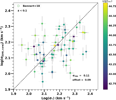
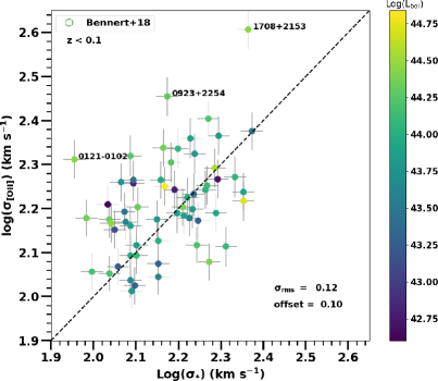
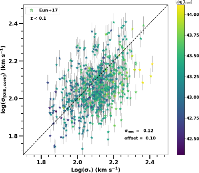
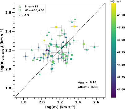
Figure 5.— Top panels: Comparison between $\rm\sigma_{*}$ and $\rm\sigma_{[OIII,core]}$ (left panel) and $\rm\sigma_{[OII]}$ (right panel) for the sample of Bennert et al. (2018), respectively. Bottom panels: Comparison between $\rm\sigma_{*}$ and $\rm\sigma_{[OIII,core]}$ for the local SDSS sample (Eun, Woo & Bae, 2017) and high redshift targets of Woo et al. (2006, 2008) and Shen et al. (2015). $\rm L_{bol}$ color-scale is displayed. The dash-line shows the one-to-one relation.

4.2. Gas and Stellar Kinematics vs. AGN Properties

For studying the relation between gas emission line width and $\sigma_{*}$ in more detail, we explored the differences between $\rm\sigma_{[OIII,core]}$ and $\sigma_{*}$ as a function of AGN properties.

Figure 6 shows the comparisons between $\rm\sigma_{[OIII,core]}$$/$$\sigma_{*}$ and $\rm M_{BH}$, $\rm L_{bol}/L_{Edd}$, $\rm L_{bol}$ and $\sigma_{*}$ for the long-slit spatially resolved spectral sample of Bennert et al. (2018). The logrithmic scale ratio of $\rm\sigma_{[OIII,core]}$$/$$\sigma_{*}$ is broadened, $\sim$-0.3$-$0.3 within a range of $\log\sigma_{*}$ = 1.8$-$2.6 (i.e., 60$-$400 km s^-1). We found that the good correlation with small scatter is shown between $\rm\sigma_{[OIII,core]}$ and $\sigma_{*}$ for those targets which have small M_BH and low $\rm L_{bol}$ i.e., $\rm\log(L_{bol}$) $<$ $\sim$43.5. While, the scatter is significantly broader when M_BH and $\rm L_{bol}$ of targets increase. In addition, we also found that for those targets which have higher $\rm L_{bol}/L_{Edd}$, $\rm\sigma_{[OIII,core]}$ tends to be larger than $\sigma_{*}$. Similar to the case of [O III] emission line, we found the good correlation between $\rm\sigma_{[OII]}$ and $\sigma_{*}$ for those targets which have small M_BH and low $\rm L_{bol}$. As $\rm L_{bol}/L_{Edd}$ increases, $\rm\sigma_{[OII]}$$/$$\sigma_{*}$ also grows (see Figure 7).

Figure 8 presents the comparisons of $\rm\sigma_{[OIII,core]}$ and $\sigma_{*}$ for the local SDSS sample. We found that those sources with low $\rm L_{bol}$ show the good correlation, while high bolometric luminosity sources show large discrepancy ($\sim$-0.4$-$0.4). Similar to the case of the long-slit spatially resolved sample of Bennert et al. (2018), $\rm\sigma_{[OIII,core]}$$/$$\sigma_{*}$ tends to increase as $\rm L_{bol}/L_{Edd}$ increases. Also, for those targets which have larger M_BH and higher $\rm L_{bol}$, $\rm\sigma_{[OIII,core]}$$/$$\sigma_{*}$ tends to be smaller when $\rm L_{bol}/L_{Edd}$ are low in those targets.

In the case of the high redshift sample, the scatter is large between $\rm\sigma_{[OIII,core]}$ and $\sigma_{*}$ ($\sim$-0.4$-$0.4). Similar to the local objects, the low bolometric luminosity sources show small scatters between $\rm\sigma_{[OIII,core]}$ and $\sigma_{*}$ compared to those high luminosity sources. And, for sources which have higher $\rm L_{bol}/L_{Edd}$, $\rm\sigma_{[OIII,core]}$$/$$\sigma_{*}$ tends to be larger (see Figure 9).

The large scatters for those high bolometric luminosity objects may indicate the difficulty in the measurement of $\rm\sigma_{*}$ for sources with large contribution of AGN emission in the center or may also illustrate an additional significant effect which broadens the [O III] emission profile (e.g., outflows), leading to large uncertainty in measuring the gravitational component such as $\rm\sigma_{[OIII,core]}$ in the [O III] profile. Particularly, $\rm L_{bol}/L_{Edd}$ seems to play an important role in the relations between NLR gas and stellar velocity dispersions.

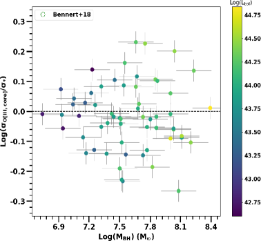
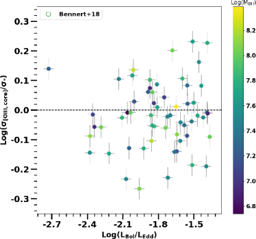
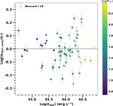
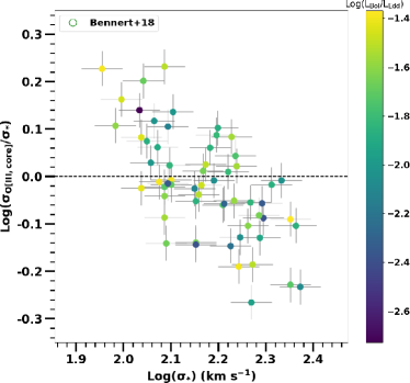
Figure 6.— Difference between $\rm\sigma_{[OIII,core]}$ and $\rm\sigma_{*}$ as a function of AGN properties, i.e., $\rm M_{BH}$, $\rm L_{bol}/L_{Edd}$, $\rm L_{bol}$, and $\rm\sigma_{*}$ for the sample of Bennert et al. (2018). The color-scale is indicated in each color map panel. The dash-line shows the one-to-one relation.

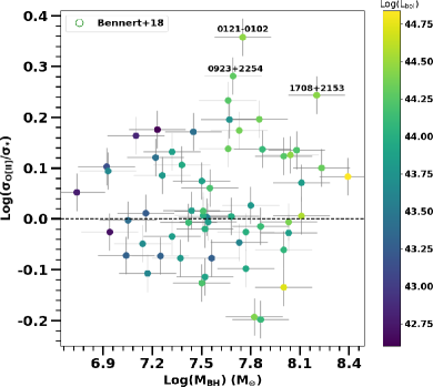
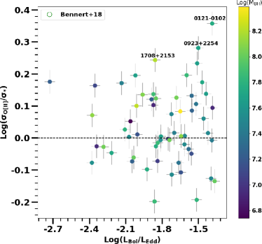
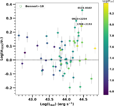
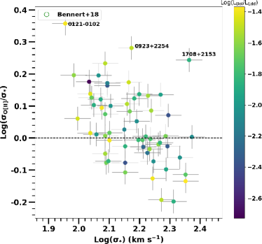
Figure 7.— Difference between $\rm\sigma_{[OII]}$ and $\rm\sigma_{*}$ as a function of AGN properties, i.e., $\rm M_{BH}$, $\rm L_{bol}/L_{Edd}$, $\rm L_{bol}$, and $\rm\sigma_{*}$ for the sample of Bennert et al. (2018). The color-scale is indicated in each color map panel. The dash-line shows the one-to-one relation.

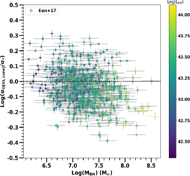
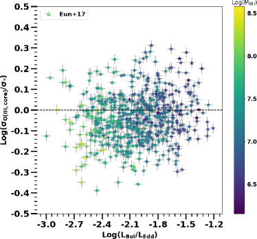
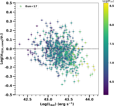
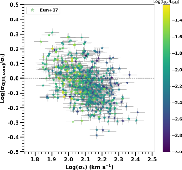
Figure 8.— Same as Figure 6 but for the local SDSS sample of Eun, Woo & Bae (2017).

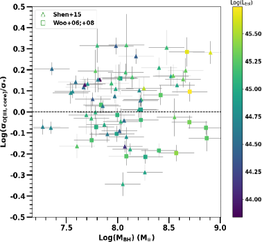
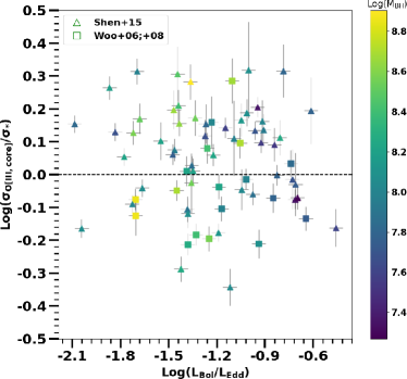
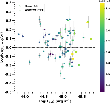
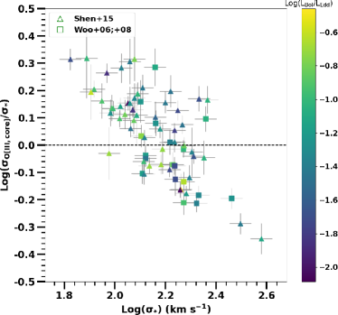
Figure 9.— Same as Figure 6 but for the high redshift sample of Woo et al. (2006, 2008) and Shen et al. (2015).

4.3. Gas and Stellar Kinematics vs. Velocity Shifts and Outflow Strengths

To study the driving factor of the discrepancy between $\rm\sigma_{[OIII,core]}$ and $\rm\sigma_{*}$, we compared the ratio $\rm\sigma_{[OIII,core]}$$/$$\sigma_{*}$ with [O III] velocity shifts ($\rm V_{[OIII,core]}$ and $\rm V_{[OIII,out]}$) and outflow strengths such as $\rm V_{max}$ and $\rm\sigma_{[OIII,out]}$.

Figure 10 presents the comparison between $\rm V_{[OIII,core]}$ and $\rm V_{[OIII,out]}$ with respect to the systemic velocity as a function of $\rm M_{BH}$ and $\rm L_{bol}$. For the sources which have low $\rm M_{BH}$ and $\rm L_{bol}$, $\rm V_{[OIII,core]}$ and $\rm V_{[OIII,out]}$ are small. And, for the sources which have higher $\rm M_{BH}$ and $\rm L_{bol}$, $\rm V_{[OIII,core]}$ and $\rm V_{[OIII,out]}$ tend to be larger with large scatter. Interestingly, the line shifts of the broad component of [O III] show blueshifted with an average velocity of $-$135$\pm$150 km s^-1; while, the line shifts of the core component display a smaller offset with an average velocity of $-$14$\pm$47 km s^-1. This result may indicate that the kinematics of the core component of [O III] and stellar absorption lines are quite close to each other, but the offsets become larger for higher $\rm M_{BH}$ and $\rm L_{bol}$ sources which have stronger outflow signatures (with larger $\rm V_{[OIII,out]}$).

In Figure 10, we also show the comparison between $\rm V_{max}$, $\rm M_{BH}$ and $\rm L_{bol}$. $\rm V_{max}$ indicates the maximum strength of the outflow component in the [O III] profile. It shows how large offset of the broad component compared to that of the core component of the [O III] emission line. We found that when $\rm L_{bol}$ increases, $\rm V_{max}$ also grows. For those targets which have small $\rm M_{BH}$ and low $\rm L_{bol}$, $\rm V_{max}$ is low. In contrast, $\rm V_{max}$ tends to be larger for objects which have higher $\rm M_{BH}$ and higher $\rm L_{bol}$. This result may indicate that the AGN accretion plays a major role in outflow physical properties.

Figure 11 shows the comparison of $\rm\sigma_{[OIII,core]}$-$\sigma_{*}$ with $\rm V_{max}$, $\rm\sigma_{[OIII,out]}$, $\rm V_{[OIII,core]}$ and $\rm V_{[OIII,out]}$, respectively. We found that when $\rm V_{max}$ increases, the discrepancy between $\rm\sigma_{[OIII,core]}$ and $\rm\sigma_{*}$ tends to be larger. Similarly, as $\rm\sigma_{[OIII,out]}$ is larger, the difference between $\rm\sigma_{[OIII,core]}$ and $\rm\sigma_{*}$ is also larger; when $\rm V_{[OIII,core]}$ and $\rm V_{[OIII,out]}$ increase, the difference between $\rm\sigma_{[OIII,core]}$ and $\rm\sigma_{*}$ also grows.

The difference between $\rm\sigma_{[OIII,core]}$ and $\rm\sigma_{*}$ is well connected with $\rm V_{max}$, $\rm\sigma_{[OIII,out]}$, $\rm V_{[OIII,core]}$ and $\rm V_{[OIII,out]}$. This result may indicate that outflows play a significant role in the discrepancy between $\rm\sigma_{[OIII,core]}$ and $\rm\sigma_{*}$.

5. Discussions

5.1. Outflow Strength Effect

The main question in our work is: what are the physically driven factors for the scatters between ionized gas kinematics in the NLR and stellar velocity dispersions? If we assume that the gas kinematics in the NLR is governed by the gravitational potential of the bulge of the host galaxy, then we expect that the velocity field of NLR emission lines should trace the same velocity field as that of the stellar velocity dispersions. However, from previous studies, many authors found that $\rm\sigma_{[OIII]}$ and $\sigma_{*}$ show correlations but with large scatters. So, what are the factors for these substantial scatters between $\rm\sigma_{[OIII]}$ and $\sigma_{*}$? As discussed in Greene & Ho (2005), the authors found that there is a strong correlation between the $\rm\sigma_{[OIII]}$$/$$\sigma_{*}$ ratio as a function of Eddington ratio, indicating that the gas kinematics of the NLR is not also governed by the primary role of the gravitational potential of the bulge but also followed by a secondary role of AGN activity such as outflows. Similar to Greene & Ho (2005), Ho (2009) found the same conclusion by analyzing the line width of the [N II] emission line. Later on, in the study of narrow-line Seyfert 1 sample, Komossa & Xu (2007) found that after correcting for the wing component in the [O III] profile, there is consistency between $\rm\sigma_{[OIII]}$ and $\sigma_{*}$. However, is there any caution in the validity of using $\rm\sigma_{[OIII,core]}$ as a surrogate for $\sigma_{*}$? To test this question, Bennert et al. (2018) used high-quality long-slit spatially resolved spectra from a sample of 52 Seyfert 1 galaxies to have a direct and simultaneous comparison between $\rm\sigma_{[OIII,core]}$ and $\sigma_{*}$. They found the large discrepancy in the comparison between object and object. So, even we use $\rm\sigma_{[OIII,core]}$ to replace $\sigma_{*}$, there is a large uncertainty to be considered.

In our study, we found the broad correlations with large scatters between $\rm\sigma_{[OIII,core]}$ and $\sigma_{*}$ for the local SDSS sample of Eun, Woo & Bae (2017). For the high redshift sample from Woo et al. (2006, 2008) and Shen et al. (2015), the correlation shows somewhat larger scatter compared to that of the local SDSS sample. By comparing the differences between $\rm\sigma_{[OIII,core]}$ and $\rm\sigma_{*}$ as a function of AGN properties, we found that $\rm\sigma_{[OIII,core]}$ and $\rm\sigma_{*}$ show small scatter in those targets which have low $\rm L_{bol}$. However, the scatter increases when $\rm L_{bol}$ grows. Particularly, we found that when $\rm L_{bol}/L_{Edd}$ increases, $\rm\sigma_{[OIII,core]}$ tends to be larger than $\rm\sigma_{*}$.

In addition, we also tested the effects of velocity shifts ($\rm V_{[OIII,core]}$ and $\rm V_{[OIII,out]}$) and outflow strengths ($\rm\sigma_{[OIII,out]}$ and $\rm V_{max}$) on the scatter between $\rm\sigma_{[OIII,core]}$ and $\sigma_{*}$. In Figures 10 and 11, we found that $\rm V_{[OIII,core]}$, $\rm V_{[OIII,out]}$, and $\rm V_{max}$ are connected with M_BH and $\rm L_{bol}$. As expected, we found that the discrepancy between $\rm\sigma_{[OIII,core]}$ and $\rm\sigma_{*}$ is also connected with $\rm V_{[OIII,core]}$ and $\rm V_{[OIII,out]}$, as well as $\rm V_{max}$ and $\rm\sigma_{[OIII,out]}$.

We also perform a Spearman’s rank-order correlation to test the relationships between [O III] vs. stellar kinematics and AGN properties. Table 2 shows the Spearman’s rank-order coefficients (r) and the p-values of the null hypothesis that the two quantities are not correlated. We found that the discrepancy between $\rm\sigma_{[OIII,core]}$ and $\rm\sigma_{*}$ has mild correlations with Eddington ratio (r = 0.16) and $\rm V_{max}$ (r = 0.17). The correlations are stronger when compared with the broad component of [O III] such as $\rm\sigma_{[OIII,out]}$ (r = 0.31) and $\rm V_{[OIII,out]}$ (r = $-$0.33). And, we also found that in comparison with $\rm\sigma_{[OIII,core]}$ and $\rm\sigma_{*}$, the discrepancy between $\rm\sigma_{[OIII,out]}$ and $\rm\sigma_{*}$ has a stronger correlation with outflow strengths such as Eddington ratio (r = 0.25) and $\rm V_{max}$ (r = 0.80). In addition, there are mild correlations when comparing the discrepancy between $\rm V_{[OIII,core]}$ and $\rm V_{*}$ with Eddington ratio (r = $-$0.24), $\rm\sigma_{[OIII,out]}$ (r = $-$0.20), and $\rm V_{max}$ (r = 0.06). In the case of $\rm V_{[OIII,out]}$ and $\rm V_{*}$, the correlations tend to be stronger with Eddington ratio (r = $-$0.29), $\rm\sigma_{[OIII,out]}$ (r = $-$0.34), and $\rm V_{max}$ (r = 0.46). Our results for the correlations between velocity shifts and Eddington ratio are in agreement with that of Zhang et al. (2011). By using homogenous samples of 383 radio-quiet Seyfert 1 galaxies, they also found that there are weak correlations between $\rm V_{[OIII,core]}$ and $\rm V_{[OIII,out]}$ with AGN properties such as $\rm L_{5100}$, M_BH, and Eddington ratio. They interpreted results that although AGN activities are responsible for launching initial outflows, the surrounding interstellar medium (ISM) environment (e.g., density profile) may also have an impact on the later speed of outflow gas after their launch, and this may lead to the diversity of [O III] properties in AGNs.

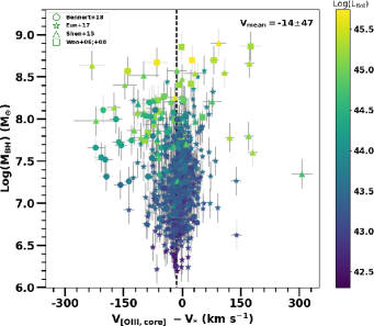
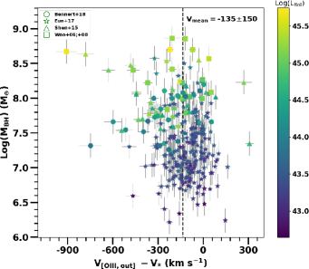
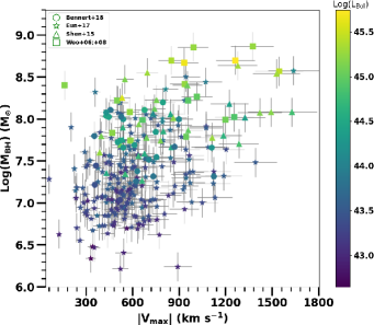
Figure 10.— Comparison between $\rm M_{BH}$ and $\rm V_{[OIII,core]}$ $-$ $\rm V_{*}$ (top panel), $\rm M_{BH}$ and $\rm V_{[OIII,out]}$ $-$ $\rm V_{*}$ (middle panel), and $\rm M_{BH}$ and $\rm V_{max}$ (bottom panel). The color scale is displayed for $\rm L_{bol}$. The samples of Bennert et al. (2018), Eun, Woo & Bae (2017), Woo et al. (2006, 2008), and Shen et al. (2015) are plotted as circle, star, square, and triangle symbols, respectively. The vertical dashed lines indicate the mean velocity shifts.

Our results are consistent with those of Greene & Ho (2005) and Ho (2009) that although gas kinematics of the NLR mainly follows the gravitational potential of the bulge of the host galaxy, AGN activities such as outflows may also have impact on the gas kinematics of the NLR. For those targets with high $\rm L_{bol}$, we expect that the AGN activity is high, and there may be strong outflows acting on the gas kinematics of the NLR, leading to the large scatter between $\rm\sigma_{[OIII,core]}$ and $\rm\sigma_{*}$. As discussed in Ho (2009), the kinematics of the NLR emission gas and stars are expected to be similar if both quantities are governed by the bulge gravitational potential. In the cases that the gas and stars suffer collisional hydrodynamic drags by the surrounding ISM, we may expect to see the results that the gas velocity dispersions are lower than that of the stars. However, if there is additional action from the AGN activity (i.e., outflows) on the relations between the gas and stars, the additional energy may accelerate the gas, then lead to the results that the gas velocity dispersions are comparable or larger than that of the stars.

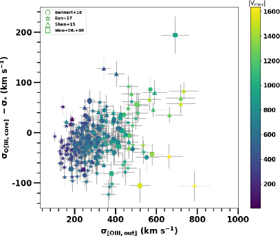
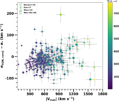
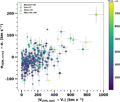
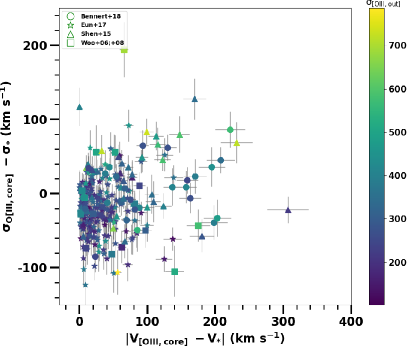
Figure 11.— Difference between $\rm\sigma_{[OIII,core]}$ and $\rm\sigma_{*}$ as a function of $\rm\sigma_{[OIII,out]}$ (top left), $\rm V_{max}$ (top right), $\rm V_{[OIII,out]}$ - $\rm V_{*}$ (bottom left), and $\rm V_{[OIII,core]}$ - $\rm V_{*}$ (bottom right). The samples of Bennert et al. (2018), Eun, Woo & Bae (2017), Woo et al. (2006, 2008), and Shen et al. (2015) are plotted as circle, star, square, and triangle symbols, respectively.

5.2. The Limitation of Double Gaussian Approach

Regarding the large scatters between $\rm\sigma_{[OIII,core]}$ and $\sigma_{*}$ for high luminosity objects, we may need to consider the details of measurement of the [O III] line width. As suggested by previous studies (e.g., Greene & Ho, 2005, Bennert et al., 2018), a double Gaussian is the best choice for fitting the [O III] profile and $\rm\sigma_{[OIII,core]}$ could be used as a surrogate for $\sigma_{*}$. But what is the true value of the gas kinematics following the gravitational potential of the stars and not disturbed by outflow effects? We have simply assumed the correction by removing the wing component in the [O III] profile. But for those high luminosity AGNs in which the fraction of AGN accretion is large, the measurement of the true $\rm\sigma_{[OIII,core]}$ as a surrogate for $\sigma_{*}$ may have high uncertainty even when we have corrected for non-gravitational effects by removing the broad wing component in the [O III] profile.

In general, we suggest that it should be cautionary to use $\rm\sigma_{[OIII,core]}$ as a surrogate for $\sigma_{*}$ for individual sources (particularly for high luminosity AGNs). The replacement of $\rm\sigma_{[OIII,core]}$ for $\sigma_{*}$ could be applied for statistical studies albeit with large scatters.

5.3. Aperture and Rotational Broadening Effects

Both gas and stellar velocity dispersions may vary with different extraction radius measurements. As we mentioned in Section 4.1, within the large aperture size of SDSS (3$\arcsec$), the extracted spectra of SDSS cover a size of $\sim$5.4 kpc in the center of the galaxy at redshift z $\sim$ 0.1. For the higher redshift sample at z $\sim$ 0.3-1.0, the radius size covers $\sim$3.3-7.8 kpc in the center of the galaxy. Within the large aperture size, it may be possible that integrated spectra of SDSS may not only extract the region within the bulge radius of the galaxy but also contain the disk component of the galaxy, then overestimate the measured velocity dispersion. Therefore, it is important to check whether the measurements of $\rm\sigma_{*}$ are well extracted within the bulge radius of the galaxy. Similarly, for the gas emission line, we should check whether the extraction radius for the [O III] emission is well defined within the NLR or not.

Greene & Ho (2005) examined the extraction aperture size of SDSS for their study based on the local type 2 AGN sample. By using the relation between the NLR radius and the [O III] luminosity, they estimated that the typical size of the NLR for their objects at z $=$ 0.1 is $\sim$0.25-1.2 kpc within the angular size of $\sim$0.14$\arcsec$-0.67$\arcsec$. This angular size is well defined within the SDSS aperture size. Following their method, we estimated the NLR size for our local SDSS and high redshift samples by using the size-luminosity relation (e.g., Bae et al., 2017, Le et al., 2017). Based on the bolometric luminosity of our sample, we estimated the [O III] luminosity of our local SDSS and high redshift samples to be in the range of $\mathrm{L_{OIII}\sim 10^{41.5}-10^{43}}$ erg s^-1($\rm L_{bol}=700\times L_{OIII}$, LaMassa et al., 2009). This luminosity range corresponds to the physical size of $\sim$0.25-3.5 kpc, well defined within the SDSS aperture size at redshift of z $\sim$ 0.1-1.0. Therefore, the measurements of the $\rm\sigma_{[OIII]}$ of our local and high redshift SDSS samples are well defined within the NLR.

As for the extraction size of $\sigma_{*}$, as discussed by Greene & Ho (2005), using the fundamental plane relation from Bernardi (2003), a median $\rm\sigma_{*}$ of 150 km s^-1 corresponds to an effective radius of $\sim$4.5 kpc. For the local SDSS sample, the integrated spectra of SDSS cover the size of $\sim$5.4 kpc at redshift of z $\sim$ 0.1. Therefore, for the local SDSS sample, the extraction size of $\rm\sigma_{*}$ is well defined within the size of the bulge of the galaxy. For the high redshift sample, the SDSS radius size includes $\sim$3.3-7.8 kpc at redshift of z $\sim$ 0.2-1.0. For the sample at high redshift z $>$ 0.5, the measurements of $\rm\sigma_{*}$ contain the light from both the bulge and disk components (see Section 4 in Shen et al., 2015), we expect that this may lead to the large scatters between $\rm\sigma_{[OIII,core]}$ and $\rm\sigma_{*}$ for the high redshift AGNs. As mentioned in Shen et al. (2015), rotational velocity could bias their measured $\rm\sigma_{*}$ ($<$16$\%$).

Greene & Ho (2005) checked the effect of rotational broadening in their sample. Based on their analysis, rotational broadening effect could overestimate the observed gas and stellar velocity dispersions in their sample by $\sim$12-15$\%$ at z $\sim$ 0.1. Accordingly, we expect that the rotational broadening effect could bias our measured gas and stellar velocity dispersions but with small fractions compared to the large scatters between $\rm\sigma_{[OIII,core]}$ and $\rm\sigma_{*}$.

For the local SDSS sample, Eun, Woo & Bae (2017) classified 221 spiral galaxies among 611 objects in their sample. Based on the minor-to-major axis ratio (b/a) obtained from the SDSS-DR7, those sources are classified into face-on (b/a $>$ 0.5) and edge-on (b/a $<$ 0.5) spiral galaxies. Figure 12 shows the comparison of $\rm\sigma_{[OIII,core]}$ and $\rm\sigma_{*}$ for the 221 spiral galaxies from the local SDSS sample. Interestingly, for those edge-on targets, we found that $\rm\sigma_{*}$ is on average ($\sim$50 km s^-1) larger than $\rm\sigma_{[OIII,core]}$. While for those face-on sources, $\rm\sigma_{[OIII,core]}$ and $\sigma_{*}$ are comparable with a scatter of $\sim$0.12 dex. Eun, Woo & Bae (2017) found that $\sigma_{*}$ for edge-on targets may be overestimated due to the contribution of the rotational velocity of the disk galaxy. In addition, for those face-on targets, the rotational velocity is relatively small compared to that of the edge-on objects. This may explain why $\sigma_{*}$ is larger than $\rm\sigma_{[OIII,core]}$ for those edge-on spiral galaxies in the local SDSS sample. Also, the rotational broadening effect may contribute less to the velocity dispersions of the NLR gas than to $\sigma_{*}$.

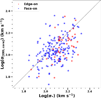
Figure 12.— Comparison between $\rm\sigma_{*}$ and $\rm\sigma_{[OIII,core]}$ for the local SDSS sample (z $<$ 0.1) of Eun, Woo & Bae (2017). The red symbols indicate edge-on targets (b/a ¡ 0.5), while, face-on targets are shown in blue symbols (b/a ¿ 0.5).

6. Summary

We constructed our sample based on four different samples at redshift z $<$ 1.0. For local AGNs (z $<$ 0.1), we selected 59 high-quality long-slit Keck spectra (Bennert et al., 2018) and 611 local hidden type 1 SDSS spectra of Eun, Woo & Bae (2017). For the higher redshift sample (0.3 $<$ z $<$ 1.0), we chose the sample which is based on 18 high S/N Keck spectra (Woo et al., 2006, 2008) and 52 co-added high S/N spectra from the SDSS-RM project (Shen et al., 2015). Consequently, our sample has the broad dynamic range of $\mathrm{\lambda L_{5100}\sim 10^{41.5}-10^{46.0}}$ erg s^-1and 6.5 $<$ $\log($M_BH) $<$ 9.5. In addition, the high S/N spectra of our sample allow us to achieve reliable measurements for $\sigma_{*}$ and $\rm\sigma_{[OIII]}$. We took advantage of this unique sample to test the validity of using $\rm\sigma_{[OIII,core]}$ as a surrogate for $\sigma_{*}$ not only for local AGNs but also for high redshift AGNs. We summarize our main results as follows:

(1) From the comparisons of $\sigma_{*}$ and $\rm\sigma_{[OIII,core]}$, we found the broad correlation between $\rm\sigma_{[OIII,core]}$ and $\sigma_{*}$ with a scatter of 0.11 dex for the local objects, while, the scatter is somewhat larger for the high redshift targets, being $\sim$0.16 dex.

(2) We found that $\rm\sigma_{[OIII,core]}$ and $\sigma_{*}$ are well correlated for the low luminosity objects, while, for the targets which have higher luminosity ranges, the scatters of correlation between $\rm\sigma_{[OIII,core]}$ and $\sigma_{*}$ become larger.

(3) We found that the Eddington ratio plays an important role in the differences between $\rm\sigma_{[OIII,core]}$ and $\sigma_{*}$. For the targets which have high Eddington ratios, $\rm\sigma_{[OIII,core]}$ tends to be larger than $\sigma_{*}$. Also, we found that outflow strengths (i.e., $\rm V_{max}$, $\rm V_{[OIII,out]}$, and $\rm\sigma_{[OIII,out]}$) have significant effects on the differences between $\rm\sigma_{[OIII,core]}$ and $\sigma_{*}$. The discrepancies between $\rm\sigma_{[OIII,core]}$ and $\sigma_{*}$ are larger when $\rm V_{max}$, $\rm V_{[OIII,out]}$, and $\rm\sigma_{[OIII,out]}$ increase.

(4) For the local SDSS sample, $\sigma_{*}$ is on average larger than $\rm\sigma_{[OIII,core]}$ for the edge-on spiral galaxies. The result may indicate that the rotational broadening effect has large contribution to $\sigma_{*}$ compared to $\rm\sigma_{[OIII]}$.

Our results show that the Eddington ratios and outflow strengths may have significant effects on the discrepancies between the gas and stellar kinematics in AGNs. Therefore, using $\rm\sigma_{[OIII,core]}$ as a surrogate for $\sigma_{*}$ should be adopted with caution, and the validity of using $\rm\sigma_{[OIII,core]}$ to replace $\sigma_{*}$ is warranted only for the low luminosity AGNs.

Table 1Targets and Measured Properties

Target	z	$\rm\lambda L_{5100}$	$\rm\sigma_{H\beta}$	$\rm\log(M_{BH})$	$\rm\sigma_{*}$	$\rm\sigma_{[OIII,core]}$	$\rm\sigma_{[OIII,out]}$	$\rm V_{max}$	$\rm V_{[OIII,core]}$	$\rm V_{[OIII,out]}$	S/N
		($\rm 10^{44}\ erg~{}s^{-1}$)	($\rm km~{}s^{-1}$)	($\rm M_{\odot}$)	($\rm km~{}s^{-1}$)	($\rm km~{}s^{-1}$)	($\rm km~{}s^{-1}$)	($\rm km~{}s^{-1}$)	($\rm km~{}s^{-1}$)	($\rm km~{}s^{-1}$)
(1)	(2)	(3)	(4)	(5)	(6)	(7)	(8)	(9)	(10)	(11)	(12)
S01………………………	0.3590	1.37	2194	8.22	132	121	314	-500	-62	-368	72
S04………………………	0.3579	1.19	1749	7.99	186	180	466	1196	-8	-8	46
S05………………………	0.3530	2.23	3333	8.70	132	118	391	-850	81	-72	119
S06………………………	0.3684	1.10	1413	7.79	169	143	412	-944	-2	-117	31
S07………………………	0.3517	1.81	2547	8.42	145	175	423	-934	22	-208	105
S08………………………	0.3585	1.59	1217	7.75	187	138	303	-586	-97	-288	54
S09………………………	0.3542	1.76	1748	8.08	187	115	181	581	-62	52	39
S11………………………	0.3558	1.57	1354	7.84	127	137	242	-467	-88	-241	115
S12………………………	0.3574	1.82	4256	8.87	173	130	579	-1327	175	-207	40
S23………………………	0.3511	1.78	4251	8.86	172	145	416	-990	-2	-120	106
S24………………………	0.3616	1.49	2635	8.40	214	141	241	-161	-10	-466	103
S26………………………	0.3691	0.83	1914	7.99	128	101	302	-661	-20	-134	50
S28………………………	0.3678	0.97	2532	8.27	210	129	379	1014	-47	-6	74
W09………………………	0.5654	2.64	2747	8.57	289	184	519	1543	-140	35	63
W11………………………	0.5650	0.78	2026	8.02	126	182	503	-1255	52	-89	18
W14………………………	0.5617	5.56	2616	8.70	228	284	506	-1263	25	-222	77
W17………………………	0.5617	0.86	2483	8.22	165	169	429	-956	4	-141	25
W22………………………	0.5622	4.65	2654	8.67	144	338	692	-932	-65	-910	82
141359.51+531049.3	0.8982	0.97	1817	7.98	121	157	0	0	-222	0	15
141324.28+530527.0	0.4559	1.07	2080	8.12	191	127	342	-739	-67	-205	381
141323.27+531034.3	0.8492	1.97	3299	8.66	166	261	0	0	172	0	14
141532.36+524905.9	0.7147	1.76	1005	7.60	182	126	285	-387	180	-165	33
141522.54+524421.5	0.5263	0.63	1229	7.54	119	146	187	4	-60	-543	48
141417.69+532810.8	0.8077	1.55	1927	8.14	232	340	0	0	-175	0	32
141151.78+525344.1	0.5165	1.16	2817	8.40	128	208	591	-952	-147	-630	62
141408.76+533938.3	0.1919	0.32	1188	7.36	82	132	248	-430	-58	-265	291
141324.66+522938.2	0.8122	1.36	2941	8.48	114	231	403	-550	0	-483	75
141724.59+523024.9	0.4818	0.90	2398	8.20	172	176	0	0	-29	0	129
141721.80+534102.6	0.1934	0.54	1025	7.35	137	115	215	551	307	307	163
141645.58+534446.8	0.4418	0.47	971	7.27	152	129	338	-660	-12	-219	72
141018.04+532937.5	0.4696	0.41	2077	7.90	130	102	236	-536	-33	-102	97
141751.14+522311.1	0.2806	0.13	3407	8.07	181	124	311	-730	6	-63	124
141112.72+534507.1	0.5872	1.35	1585	7.94	97	133	356	-638	-72	-348	39
140943.01+524153.1	0.4211	0.40	2268	7.97	184	219	0	0	33	0	108
141409.44+535648.2	0.8251	1.36	1264	7.74	95	88	357	-778	-65	-203	195
141941.11+533649.6	0.6457	3.52	1767	8.25	109	142	261	-531	-19	-157	93
142010.25+524029.6	0.5477	0.91	3681	8.58	177	237	0	0	-14	0	68
141004.27+523141.0	0.5266	1.28	2248	8.23	150	173	159	754	-77	268	147
142038.52+532416.5	0.2647	0.24	2633	7.98	66	137	0	0	-73	0	183
141658.28+521205.1	0.6018	2.01	3184	8.64	158	227	719	-1276	-231	-783	63
141514.15+540222.9	0.8488	1.97	2910	8.55	201	190	324	-694	109	-29	60
142043.53+523611.4	0.3368	0.24	2034	7.76	115	133	289	-535	-65	-272	167
141320.05+520527.9	0.5998	0.87	2590	8.26	313	182	0	0	-1	0	378
142124.36+532312.5	0.8255	1.21	1813	8.03	225	203	0	0	-71	0	40
142112.29+524147.3	0.8425	1.52	1818	8.09	77	161	734	-1491	-99	-444	91
141031.33+521533.8	0.6076	1.14	1388	7.78	187	186	348	-687	-106	-313	149
141049.76+540040.6	0.8343	1.16	1247	7.69	154	149	364	-521	-18	-432	23
142209.14+530559.8	0.7542	4.35	3532	8.91	106	203	0	0	93	0	11
141058.78+520712.2	0.3910	0.26	3249	8.18	93	170	477	1224	-113	-113	224
141852.64+520142.8	0.4398	0.31	1713	7.67	96	126	331	850	-26	-26	52
141553.09+541816.5	0.7305	1.86	1218	7.78	80	126	584	-1113	122	-361	32
140904.43+540344.2	0.6585	0.87	3478	8.52	215	318	0	0	-99	0	31
141115.19+515209.0	0.5716	1.45	1822	8.08	123	189	565	1420	-115	-115	37
141135.89+515004.5	0.6500	1.30	1365	7.80	119	247	343	-397	170	-313	19
140715.49+535610.2	0.6827	2.02	2851	8.54	119	177	719	-1528	33	-244	78
140551.99+533852.1	0.4548	0.64	2291	8.08	197	150	662	1625	-50	19	139
140923.42+515120.1	0.8532	1.07	1915	8.05	379	172	337	-520	184	-161	8
141419.84+533815.3	0.1645	0.70	1446	7.71	98	134	663	-1284	10	-404	91
140915.70+532721.8	0.2584	0.35	3147	8.22	172	195	0	0	-73	0	86
141253.92+540014.4	0.1871	0.09	2431	7.68	117	158	0	0	-9	0	191
140759.07+534759.8	0.1725	0.40	1995	7.86	130	139	418	796	-61	-337	146
140812.09+535303.3	0.1161	0.07	3076	7.83	112	160	0	0	-3	0	274
142103.53+515819.5	0.2634	0.35	1521	7.59	105	146	317	-675	-62	-200	107
141318.96+543202.4	0.3623	0.98	1592	7.87	130	113	399	-956	-123	-192	82
141644.17+532556.1	0.4253	0.43	1843	7.81	114	163	462	1185	-92	-92	127
141729.27+531826.5	0.2374	0.31	2695	8.06	204	186	465	-844	-100	-445	86
142100.04+532139.6	0.6766	1.57	1657	8.01	89	129	390	-862	-13	-151	27
141308.10+515210.4	0.2882	0.54	1307	7.56	104	130	329	-638	-78	-285	68
141645.15+542540.8	0.2439	0.25	2733	8.02	164	134	465	1323	-55	83	118
142225.62+533426.3	0.7569	0.57	2717	8.21	144	183	0	0	77	0	10

Note. — Col. (1): Name of target. Col. (2): Redshift. Col. (3): Continuum luminosity at 5100Å. Col. (4): Line dispersion of $\rm{H\beta}$ emission line. Col. (5): Black-hole mass. Col (6): Stellar velocity dispersion. Col. (7): Line dispersion of the core component of [O III] emission line. Col. (8): Line dispersion of the broader component of [O III] emission line. Col. (9): Outflow velocity. Col. (10): Velocity shift of the core component of [O III] emission line with respect to the stellar systemic velocity. Col. (11): Velocity shift of the broader component of [O III] emission line with respect to the stellar systemic velocity. Col. (12): Signal-to-noise ratio of spectra at 5100Å continuum. Error values are 0.04 dex for all measured properties (except that black-hole mass uncertainty is 0.4 dex).

Table 2Spearman’s rank-order Correlation Results between [O III] vs. Stellar Kinematics and AGN Properties

	$\rm\log(M_{BH})$	$\rm\log(L_{Bol}/L_{Edd})$	$\rm\log(\lambda L_{5100}$)	$\rm V_{max}$	$\rm\sigma_{[OIII,out]}$	$\rm V_{[OIII,out]}$ - $\rm V_{*}$	$\rm V_{[OIII,core]}$    - $\rm V_{*}$	$\rm\sigma_{[OIII,core]}$ - $\rm\sigma_{*}$	$\rm\sigma_{[OIII,out]}$ - $\rm\sigma_{*}$
	($\rm M_{\odot}$)		($\rm 10^{44}\ erg~{}s^{-1}$)	($\rm km~{}s^{-1}$)	($\rm km~{}s^{-1}$)	($\rm km~{}s^{-1}$)	($\rm km~{}s^{-1}$)	($\rm km~{}s^{-1}$)	($\rm km~{}s^{-1}$)
	(1)	(2)	(3)	(4)	(5)	(6)	(7)	(8)	(9)
$\rm\sigma_{[OIII,core]}$ $-$ $\rm\sigma_{*}$	$-$0.11 (5e$-$03)	0.16 (9e$-$06)	$-$0.08 (3e$-$02)	0.17 (3e$-$03)	0.31 (4e$-$08)	$-$0.33 (6e$-$09)	$-$0.09 (1e$-$02)	1.00 (0e+00)	0.53 (8e$-$23)
$\rm\sigma_{[OIII,out]}$ $-$ $\rm\sigma_{*}$	0.29 (3e$-$07)	0.25 (1e$-$05)	0.35 (5e$-$10)	0.80 (3e$-$67)	0.94 (2e$-$140)	$-$0.34 (2e$-$09)	$-$0.20 (6e$-$04)	0.53 (8e$-$23)	1.00 (0e+00)
$\rm V_{[OIII,core]}$ $-$ $\rm V_{*}$	0.03 (4e$-$01)	$-$0.24 (1e$-$10)	$-$0.11 (3e$-$03)	0.06 (3e$-$01)	$-$0.20 (6e$-$04)	0.30 (1e$-$07)	1.00 (0e+00)	$-$0.09 (1e$-$02)	$-$0.20 (6e$-$04)
$\rm V_{[OIII,out]}$ $-$ $\rm V_{*}$	$-$0.15 (9e$-$03)	$-$0.29 (4e$-$07)	$-$0.31 (5e$-$08)	0.46 (2e$-$17)	$-$0.34 (2e$-$09)	1.00 (0e+00)	0.30 (1e$-$07)	$-$0.33 (6e$-$09)	$-$0.34 (2e$-$09)

Note. — Col. (1): Black-hole mass. Col. (2): Eddington ratio. Col. (3): Continuum luminosity at 5100Å. Col. (4): Outflow velocity. Col. (5): Line dispersion of the broader component of [O III] emission line. Col (6): Velocity shift of the broader component of [O III] emission line with respect to the stellar systemic velocity. Col. (7): Velocity shift of the core component of [O III] emission line with respect to the stellar systemic velocity. Col. (8): Line dispersion of the core component of [O III] emission line with respect to the stellar dispersion. Col. (9): Line dispersion of the broad component of [O III] emission line with respect to the stellar dispersion. The p-values of the null hypothesis that the two quantities are not correlated are shown in parentheses, following the Spearman’s rank-order coefficients. The outflow velocities are used in absolute values for comparing with the line dispersions. The numbers of the sources in the correlation calculations for the core and broad components of [O III] emission line are 740, and 300, respectively.

References

- Abazajian et al. (2009) Abazajian, K. N., Adelman-McCarthy, J. K., Agüeros, M. A., et al. 2009, ApJS, 182, 543
- Ayubinia et al. (2022) Ayubinia, A., Xue, Y. Q., Woo, J-.H. et al. 2022, Universe, in press
- Bae & Woo (2014) Bae, H.-J., & Woo, J.-H. 2014, ApJ, 795, 30
- Bae et al. (2017) Bae, H-J., Woo, J.-H., Karouzos, M. et al. 2017, ApJ, 837, 91
- Bernardi (2003) Bernardi, M. 2003, AJ, 125, 1866
- Bennert et al. (2018) Bennert V. N. et al., 2018, MNRAS, 481, 138
- Bennert et al. (2015) Bennert V. N. et al., 2015, ApJ, 809, 20
- Bennert et al. (2010) Bennert, V. N., Treu, T., Woo, J.-H., et al. 2010, ApJ, 708, 1507
- Bentz et al. (2006) Bentz, M. C., Peterson, B. M., Pogge, R. W., Vestergaard, M., & Onken, C. A. 2006, ApJ, 644, 133
- Bentz et al. (2009a) Bentz, M. C., Peterson, B. M., Netzer, H., Pogge, R. W., & Vestergaard, M. 2009, ApJ, 697, 160
- Bentz et al. (2013) Bentz, M. C., Denney, K. D., Grier, C. J., et al. 2013, ApJ, 767, 149
- Boroson (2003) Boroson, T. A., 2003, ApJ, 585, 647
- Boroson & Green (1992) Boroson, T. A., & Green, R. F. 1992, ApJS, 80, 109
- Boroson (2005) Boroson, T. 2005, AJ, 130, 381
- Bonning et al. (2005) Bonning, E.W., Shields, G. A., Salviander, S., McLure, R. J., 2005, ApJ, 626, 89
- Cappellari & Emsellem (2004) Cappellari, M., & Emsellem, E. 2004, PASP, 116, 138
- Crenshaw & Kraemer (2000) Crenshaw, D. M., & Kraemer, S. B. 2000, ApJL, 532, L101
- Eun, Woo & Bae (2017) Eun, D., Woo, J.-H. & Bae, H.-J. 2017, ApJ, 842, 5
- Eracleous & Halpern (2004) Eracleous, M. & Halpern, J. P. 2004, ApJS, 150, 181
- Ferrarese & Merrit (2000) Ferrarese, L., & Merritt, D. 2000, ApJ, 539, L9
- Gebhardt et al. (2000) Gebhardt, K., Bender, R., Bower, G., et al. 2000, ApJ, 539, L13
- Greene & Ho (2005) Greene, J. E., & Ho, L. C. 2005a, ApJ, 627, 721
- Grupe & Mathur (2004) Grupe, D. & Mathur, S., 2004, ApJ, 606, L41
- Harris et al. (2012) Harris, C. E., Bennert V. N., Auger M. W., Treu T., Woo J.-H., Malkan M. A., 2012, ApJS, 201, 29
- Harrison et al. (2014) Harrison, C. M., Alexander, D. M., Mullaney, J. R., Swinbank, A. M., 2014, MNRAS, 441, 3306
- Heckman et al. (1984) Heckman, T. M., Miley, G. K., & Green, R. F. 1984, ApJ, 281, 525
- Ho (2009) Ho, L. C. 2009, ApJ, 699, 638
- Hu et al. (2008) Hu, C., Wang, J. M., Ho, L. C. et al. 2008, ApJ, 687, 78
- Komossa & Xu (2007) Komossa, S. & Xu, D., 2007, ApJ, 667, L33
- Komossa et al. (2008) Komossa, S., Xu, D., Zhou, H., Storchi-Bergmann, T., & Binette, L. 2008, ApJ, 680, 926
- Kormendy & Ho (2013) Kormendy, J., & Ho, L. C. 2013, ARA&A, 51, 511
- LaMassa et al. (2009) LaMassa, S. M., Heckman, T. M., Ptak, A., et al. 2009, ApJ, 705, 568
- Le et al. (2014) Le, H. A. N., Pak, S., Im, M., et al. 2014, JASR, 54, 6
- Le et al. (2017) Le, H. A. N., Woo, J-.H., Karouzos, M. et al. 2017, ApJ, 851, 8
- Le & Woo (2019) Le, H. A. N. & Woo, J-.H. 2019, ApJ, 887, 246
- Le, Woo & Xue (2020) Le, H. A. N., Woo, J-.H., & Xue, Y. Q. 2020, ApJ, 901, 35
- Lin et al. (2022) Lin, X., Xue, Y. Q., Fang, G. et al. 2022, RAA, 22, 015010
- McLure & Dunlop (2004) McLure, R. J., & Dunlop, J. S. 2004, MNRAS, 352, 1390
- McLure & Jarvis (2002) McLure, R. J., & Jarvis, M. J. 2002, MNRAS, 337, 109
- Nelson & Whittle (1996) Nelson, C. H. & Whittle, M., 1996, ApJ, 465, 96
- Nelson (2000) Nelson, C. H., 2000, ApJ, 544, 91
- Netzer & Trakhtenbrot (2007) Netzer, H., Trakhtenbrot, B., 2007, ApJ, 654, 754
- Oke et al. (1995) Oke, J. B., Cohen, J. G., Carr, M., et al. 1995, PASP, 107, 375
- Park et al. (2015) Park, D., Woo, J.-H., Bennert, V. et al. 2015, ApJ, 799, 164
- Peng et al. (2006) Peng, C. Y., Impey, C. D., Rix, H.-W., et al. 2006, ApJ, 649, 616
- Phillips et al. (1986) Phillips, M. M., Jenkins, C. R., Dopita, M. A., Sadler, E. M., & Binette, L. 1986, AJ, 91, 1062
- Rice et al. (2006) Rice, M., Martini, P., Greene J. E., Pogge, R. W., Shields J. C., Mulchaey, J. S., Regan, M. W., 2006, ApJ, 636, 654
- Salviander et al. (2007) Salviander, S., Shields, G. A., Gebhardt, K., & Bonning, E. W. 2007, ApJ, 662, 131
- Salviander & Shields (2013) Salviander, S. & Shields, G. A, 2013, ApJ, 662, 13
- Salviander, Shields & Bonning (2015) Salviander, S., Shields, G. A., Bonning, E. W., 2015, ApJ, 799, 173
- Shankar et al. (2016) Shankar, F., Bernardi, M., Sheth, R. K., et al. 2016, MNRAS, 460, 3119
- Shankar et al. (2019) Shankar, F., Weinberg, D. H., Marsden, C. et al. 2019, MNRAS, 493, 1500
- Shen et al. (2015) Shen, Y. et al. 2015, ApJ, 805, 96
- Shen et al. (2016) Shen, Y. et al. 2016, ApJ, 831, 7
- Shields et al. (2003) Shields, G. A., Gebhardt, K., Salviander, S., Wills, B. J., Xie, B., Brotherton, M. S., Yuan, J., & Dietrich, M. 2003, ApJ, 583, 124
- Silk & Rees (1998) Silk, J., & Rees, M. J. 1998, A&A, 331, L1
- Sexton et al. (2020) Sexton, R. O., Matzko, W., Darden, N., Canalizo, G., & Gorjian, V. 2020, MNRAS, 500, 2871
- Sun et al. (2015) Sun, M., Trump, J. R., Brandt, W. N., et al. 2015, ApJ, 802, 14
- Terlevich, Diaz & Terlevich (1990) Terlevich, E., Diaz, A. I., Terlevich, R., 1990, MNRAS, 242, 271
- Trakhtenbrot & Netzer (2012) Trakhtenbrot, B., & Netzer, H. 2012, MNRAS, 427, 3081
- Tremaine et al. (2002) Tremaine, S., Gebhardt, K., Bender, R., et al. 2002, ApJ, 547, 2
- Valdes et al. (2004) Valdes, F., Gupta, R., Rose, J. A., Singh, H. P., & Bell, D. J. 2004, ApJS, 152, 251
- Wang & Lu (2001) Wang, T. & Lu, Y. 2001, A&A, 377, 52
- Wilson & Heckman (1985) Wilson, A. S., & Heckman, T. M. 1985, in Astrophysics of Active Galaxies and Quasi-Stellar Objects, ed. J. S. Miller (Mill Valley: University Science Books), 39
- Whittle (1992) Whittle, M., 1992, ApJ, 387, 109
- Woo et al. (2006) Woo, J.-H., Treu, T., Malkan, M. A., & Blandford, R. D. 2006, ApJ, 645, 900
- Woo et al. (2008) Woo, J.-H., Treu, T., Malkan, M. A., & Blandford, R. D. 2008, ApJ, 681, 925
- Woo et al. (2010) Woo, J.-H., Treu, T., Barth, A. J., et al. 2010, ApJ, 716, 269
- Woo et al. (2015) Woo, J.-H., Yoon, Y., Park, S. et al. 2015, ApJ, 801, 38
- Woo et al. (2016) Woo, J.-H., Bae, H.-J., Son, D., & Karouzos, M. 2016, ApJ, 817, 108
- Woo et al. (2018) Woo, J.-H., Le, H. A. N., Karouzos, M., et al. 2018, ApJ, 859, 138
- Woo et al. (2019) Woo, J.-H., Cho, H., Gallo, E., et al. 2019, Nature Astronomy, 3, 755
- Xue et al. (2010) Xue, Y. Q., Brandt, W. N., Luo, B., et al. 2010, ApJ, 720, 368
- Xue (2017) Xue, Y. Q. 2017, NewAR, 79, 59
- York et al. (2000) York, D. G., Adelman, J., Anderson, Jr., J. E., et al. 2000, AJ, 120, 1579
- Zamanov et al. (2002) Zamanov, R., Marziani, P., Sulentic, J. W., et al. 2002, ApJL, 576, L9
- Zhang et al. (2011) Zhang, K., Dong, X-. B., Wang, T-. G. & Gaskell, C. M. 2011, ApJ, 737, 71