Adaptation maximizes information and minimizes dissipation across biological scales

Abstract

Biological and living systems possess the inherent capacity to process information across spatiotemporal scales, displaying the hallmark ability to constantly adapt their responses to ever-changing and complex environments. In this work, we show that adaptation is a fundamental mechanism that spontaneously emerges when the system seeks to both maximize its information on external environments and minimize the unavoidable dissipation of its receptors. Adaptive responses arise in a narrow optimal regime characterized by such information-dissipation trade-off and a maximal information gain over time. Surprisingly, in systems close to optimality, the dynamics of adaptation reveals that the information gain is necessarily tangled with a reduction of the entropy produced by microscopic processes and an increase in the efficacy of feedback mechanisms. Moreover, we demonstrate that adaptation necessarily requires the simultaneous presence of negative feedback and a slow mechanism of information storage, while being independent of biological details. Finally, we employ our framework to investigate large-scale neural adaptation in zebrafish larvae subjected to repeated visual stimulation, paving the way for the understanding of the essential mechanisms that underlie adaptive behaviors and information processing in biological and living systems.

Sensing and adaptation mechanisms in biological systems span a wide range of temporal and spatial scales, from cellular to multi-cellular level, forming a basis for decision-making and the optimization of limited resources [1, 2, 3, 4, 5, 6, 7, 8]. Prominent examples include the modulation of flagellar motion operated by bacteria according to changes in the local nutrient concentration [9, 10, 11], the regulation of immune responses through feedback mechanisms [12, 13], and the maintenance of high sensitivity in varying environments for olfactory or visual sensing in mammalian neurons [14, 15, 16, 17, 18].

In the last decade, advances in experimental techniques fostered the quest for the core biochemical mechanisms governing information processing. Simultaneous recordings of hundreds of biological signals made it possible to infer distinctive features directly from data [19, 20, 21, 22]. However, many approaches fall short of describing the connection between the underlying chemical processes and the observed behaviors [23, 24, 25, 26]. As a step in this direction, a multitude of works focused on the architecture of specific signaling networks, from tumor necrosis factor [12, 13] to chemotaxis [9, 27], highlighting the essential structural ingredients for their efficient functioning. An observation shared by the majority of these studies is the key role of a negative feedback mechanism to induce an emergent adaptive response [28, 29, 30, 31].

Any information-processing system, biological or not, must obey information-thermodynamic laws that prescribe the necessity of a storage mechanism [32], an unavoidable feature compatible with the structure of numerous chemical signaling networks [9, 28]. The storage of information consumes energy during processing [33, 34], implying that general sensing mechanisms have to take place out-of-equilibrium [3, 35, 36, 37]. The recent discovery of memory molecules in different contexts [38, 39, 40] hints at a possible implementation of storing mechanisms directly at the molecular scale, providing a microscopic dynamical memory that lays the biochemical foundation for the emergence of adaptive responses at different biological scales.

Consequently, negative feedback, storage mechanisms, and out-of-equilibrium conditions seem to be necessary requirements for a system to process environmental information and consequently adapt. At both sensory and molecular levels, adaptation manifests as a progressive decay in the amplitude of the response to repeated or prolonged stimulation. In these terms, it is manifestly a ubiquitous phenomenon, from biochemical concentrations [41, 42, 43] to populations of neurons [44, 45, 46]. Due to its universality, the aforementioned ingredients driving adaptation should be independent of the specific spatiotemporal scales and chemical pathways through which the system of interest operates. However, a comprehensive framework linking the microscopic processes implementing these mechanisms and the emergent macroscopic features is still elusive.

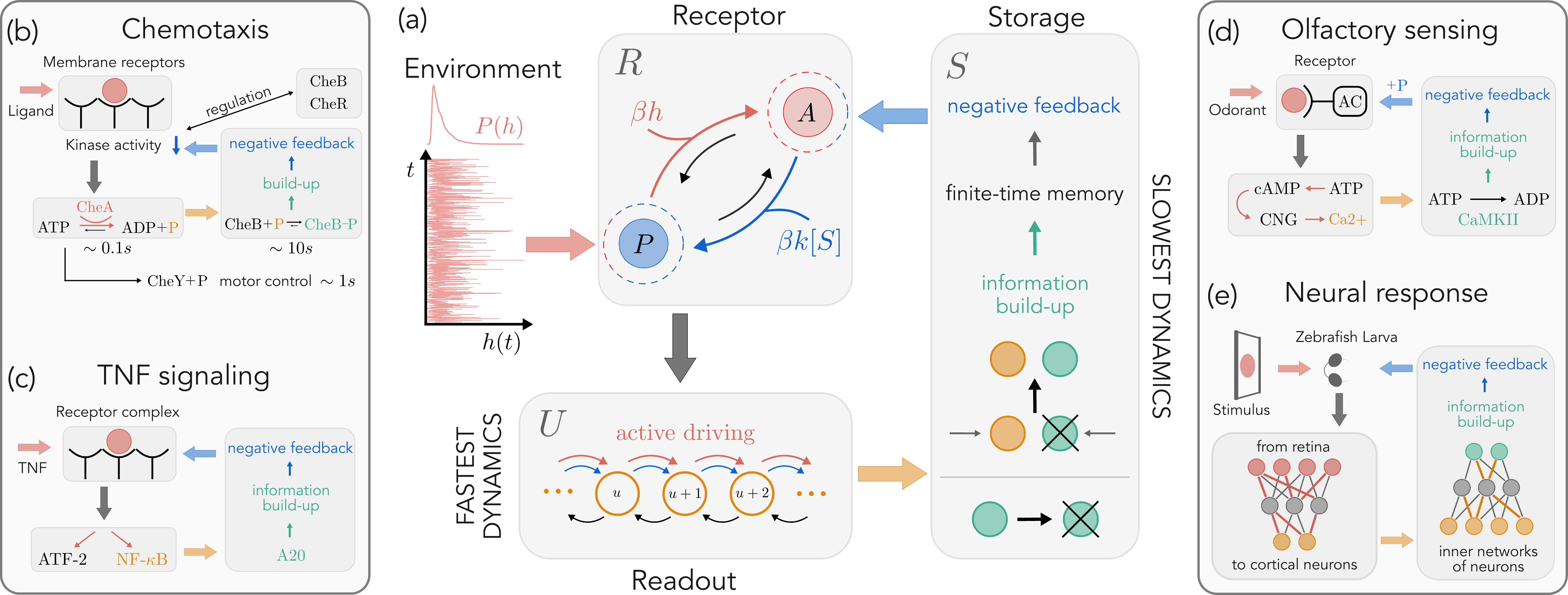
Figure 1: Sketch of the model architecture and biological examples at different scales. (a) A receptor $R$ can be either in an active ($A$) or passive ($P$) state, with transitions following two pathways, one used for sensing (red) and affected by the environment $h$, and the other (blue) modified by the storage concentration, $[S]$. An active receptor increases the response of a readout population $U$ (orange), which in turns stimulates the production of storage molecules $S$ (green) that provide a negative feedback to the receptor. (b) In chemotaxis, the input ligand binds to membrane receptors, regulating motor control and producing phosphate groups, whose concentration regulates the receptor methylation level. (c) Similarly, in tumor necrosis factor (TNF) signaling the nuclear factor $NF-\kappa B$ is produced after receptor binding to TNF. $NF-\kappa B$ modulates the encoding of the zinc-finger protein A20, which closes the feedback loop by inhibiting the receptor complex. (d) In olfactory sensing, odorant binding induces the activation of adenylyl cyclase (AC). AC stimulates a calcium flux, eventually producing phosphorylase calmodulin kinase II (CAMKII) which phosphorylates and deactivates AC. (e) In neural response, multiple mechanisms may take place at different scales. In zebrafish larvae, visual stimulation is projected along the visual stream from the retina to the cortex, a coarse-grained realization of the $R$-$U$ dynamics. Inhibitory populations and molecular mechanisms, such as short-term synaptic depotentiation, are responsible for an adapted response upon repeated stimulation.

In this work, we design a novel archetypal model for sensing to study the conditions upon which adaptive responses emerge from the underlying processes. Our scheme resolves the minimal ingredients needed to implement energy consumption, negative feedback, and storage mechanisms, providing striking analogies with real biological networks across different scales. By deriving an exact solution of the model, we identify the key mechanisms driving adaptation - negative feedback provided by slow information storage. We find that adaptation is a fundamental process through which the system dynamically builds up information on the environment while reducing internal dissipation. This twofold advantage appears in a narrow optimal region of parameters characterized by an information-dissipation trade-off, constraining the range of operations of any biological system. We finally test our ideas at the mesoscopic scale of neural responses of zebrafish larvae subjected to repeated visual stimuli, hinting at a possible functional role of the observed adaptive behavior in real-world scenarios.

I Archetypal model for sensing in biological systems

We describe a receptor $R$ that can be either active ($r=1$) or passive ($r=0$), with the two states separated by an energetic barrier $\Delta E=E_{A}-E_{P}>0$ (Figure 1a). The receptor undergoes spontaneous transitions between the passive and active states and it is stimulated by an external signal $h(t)$, the input to be encoded by the system. The environment, described by a time-dependent probability distribution $p_{H}(h,t)$, acts as a non-equilibrium energetic driving that favors activation. Conversely, inhibition takes place through a negative feedback process mediated by the concentration of a chemical population $S$. Its role is to store information about the external signal and use it to limit further activation of the sensing network.

Activation triggered by the environmental signal acts along a “sensing pathway” (superscript $H$), while the inhibition mechanism affects the “internal pathway” (superscript $I$) between the receptor’s states. This choice represents a coarse-grained description of the different chemical networks that realize these two processes. Reaction rates follow the standard Arrhenius’ law:

$$\Gamma_{P\to A}^{(H)}=e^{\beta(h-\Delta E)}\Gamma^{0}_{H}\quad\quad \Gamma_{A\to P}^{(H)}=\Gamma^{0}_{H}$$ (1)

$$\Gamma_{P\to A}^{(I)}=e^{-\beta\Delta E}\Gamma^{0}_{I}\quad\quad \Gamma_{A\to P}^{(I)}=\Gamma^{0}_{I}e^{\beta z(s/N_{S})}$$

where $\Gamma^{0}_{H}$ and $\Gamma^{0}_{I}$ set the timescales of the two pathways. Inhibition of the receptor, $\Gamma_{A\to P}^{(I)}$, depends on the concentration of $S$ at a given time through a function $z(s/N_{S})$, where $N_{S}$ is the maximum number of storage molecules available. Crucially, the presence of two different transition pathways creates an internal non-equilibrium cycle in receptor dynamics (see Appendix A).

The receptor actively drives the production of a readout population $U$, which represents the direct response of the system to external environmental signals. As such, we consider it to be the observable that characterizes adaptive behaviors. It may describe, at different scales, phosphate molecules for chemotactic response [9, 27], the nuclear factor in TNF signaling networks [12, 13], calcium for olfactory sensing mechanisms [14, 15], or photoreceptors for visual sensing [16, 17, 18] (Figures 1b-e). In full generality, we model the dynamics of both readout and storage populations with birth-and-death master equations. In particular, the dynamics of $U$ is given by:

$$\varnothing_{U}\to U\qquad U\to\varnothing_{U}$$ (2)

$$\Gamma_{u\to u+1}=e^{-\beta(V-cr)}\Gamma^{0}_{U}\quad\quad \Gamma_{u+1\to u}=(u+1)\Gamma^{0}_{U}$$

where $u$ denotes the number of molecules, $V$ is the energy needed to produce a readout unit, $c$ the receptor-induced driving, and $\Gamma^{0}_{U}$ sets the process timescale. Hence, active receptors transduce the environmental energy into an active pumping on the readout node, allowing readout molecules to encode information on the external signal.

In turn, readout units catalyze the production of a storage population $S$, whose number of molecules $s$ is described by:

$$U+\varnothing_{S}\to U+S\qquad S\to\varnothing_{S}$$ (3)

$$\Gamma_{s\to s+1}=ue^{-\beta\sigma}\Gamma^{0}_{S}\quad\quad \Gamma_{s+1\to s}=(s+1)\Gamma^{0}_{S}$$

where $\sigma$ is the energetic cost of a storage unit, $\Gamma^{0}_{S}$ sets its timescale, and $s=N_{S}$ is a reflective boundary. A depletion of readout molecules by storage production will not change the results, since, as we will see, the dynamics of $U$ is the fastest one. $S$ may model phosphorylated methylesterase (CheB-P) in chemotactic networks [27], the zinc-finger protein in TNF signaling [12], memory molecules sensitive to calcium activity [38], and synaptic depotentiation, or, at a more coarse-grained scale, neural populations that regulate neuronal response (Figure 1b-e). Storage molecules, as we will see, are responsible for encoding the readout response and play the role of a finite-time memory. For simplicity, in Eq. (1) we choose $z(s/N_{S})=\kappa\sigma s/N_{S}$, where $\kappa$ is a proportionality constant that sets the inhibition strength.

In the complete architecture (Figure  1a), four different timescales are at play, one for receptors, $\tau_{R}$, one for the readout, $\tau_{U}$, one for the storage, $\tau_{S}$, and another for the environment, $\tau_{H}$. We employ the biologically plausible assumption that $U$ undergoes the fastest evolution, while $S$ and $H$ are the slowest degrees of freedom [27, 47], i.e., $\tau_{U}\ll\tau_{R}\ll\tau_{S}\sim\tau_{H}$. Importantly, this model can be declined to analyze systems at very different scales. The chemically consistent structure of its rates allows us to directly describe reactions taking place at the molecular scale of biochemical networks (Figure 1b-d). However, we may as well assume that the dynamics of receptors, readout, and storage represent a coarse-grained, macroscopic description without specific biological details in mind (Figure 1e). Thus, on the one hand, this minimal model contains the microscopic ingredients needed to implement dissipative effects, negative feedback, and storage mechanisms. On the other hand, it allows us to tackle the general features shared across biological scales, and in particular to understand under which conditions the system is able to adapt to external changes in the environment $H$.

II Adaptation as an information-dissipation trade-off

II.1 Optimal responses in a constant environment

The system dynamics is governed by four different operators, $\hat{W}_{X}$, with $X=R,U,S,H$, one for each chemical species, and one for the external field. The resulting master equation is:

$$\partial_{t}P=\left[\frac{\hat{W}_{R}(s,h)}{\tau_{R}}+\frac{\hat{W}_{U}(r)}{\tau_{U}}+\frac{\hat{W}_{S}(u)}{\tau_{S}}+\frac{\hat{W}_{H}}{\tau_{H}}\right]P\;,$$ (4)

where $P$ denotes, in general, the joint propagator $P(u,r,s,h,t|u_{0},r_{0},s_{0},h_{0},t_{0})$, with $u_{0}$, $r_{0}$, $s_{0}$ and $h_{0}$ initial conditions at time $t_{0}$. The intrinsic timescale separation, i.e., the biologically plausible assumption that in our model one must take

$$\Gamma^{0}_{S}\ll\Gamma^{0}_{I}\approx\Gamma^{0}_{H}\ll\Gamma^{0}_{U},$$

allows us to find an exact self-consistent solution to Eq. (4) at all times $t$ (see Appendix B and Supplementary Information). To maintain analytical tractability, we choose an exponentially distributed environment $p_{H}(h,t)\sim\exp\left[-h/\expectationvalue{H}(t)\right]$, where $\expectationvalue{H}$ is the possibly time-dependent average environmental signal.

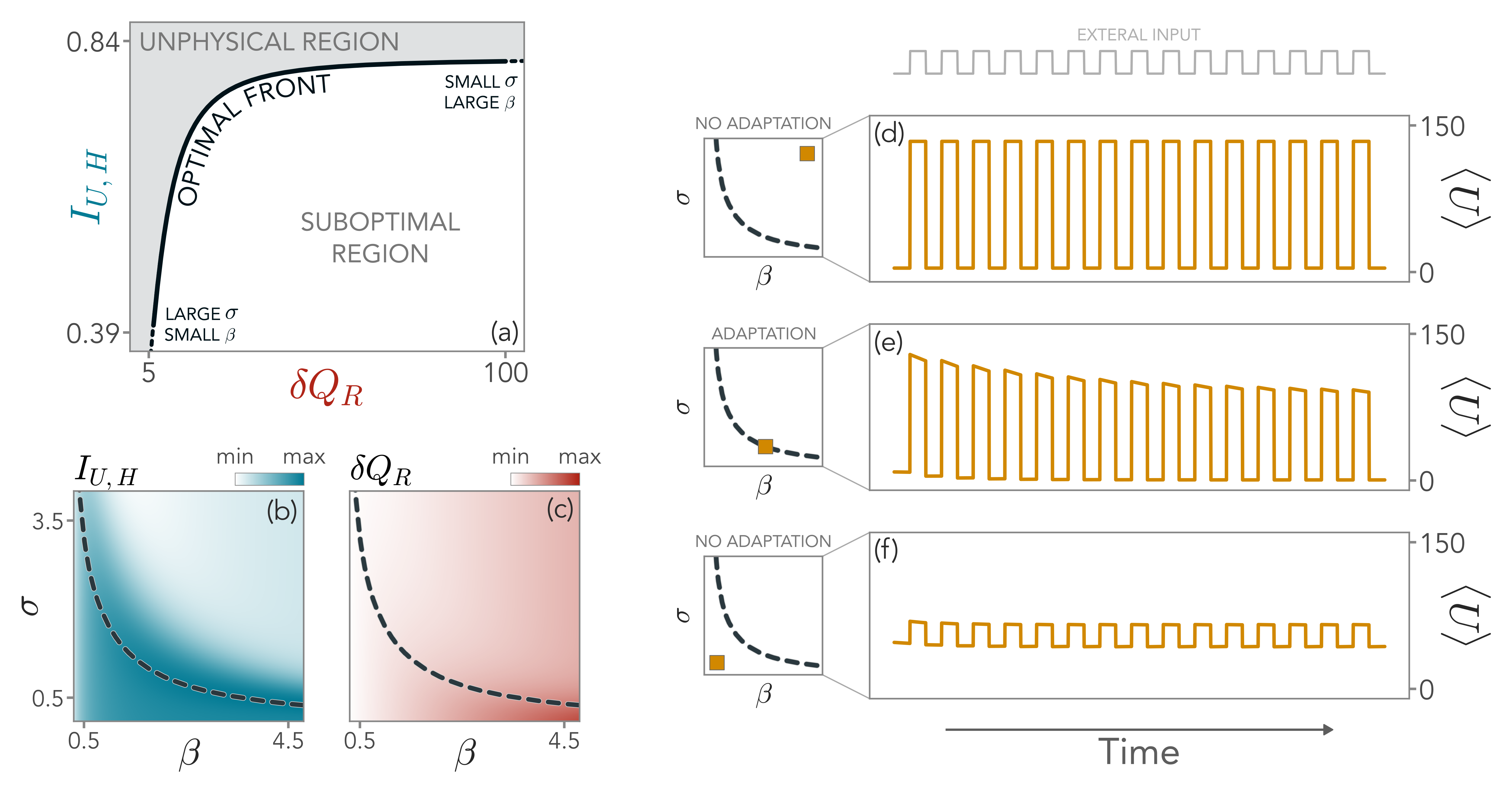
Figure 2: Adaptation emerges as an information-dissipation trade-off. (a) Pareto front (black line) in the features space that minimizes receptor dissipation, $\delta Q_{R}$, and maximizes encoded information on the signal $H$ by the readout $U$, $I_{U,H}$. Below the front, the system exploits the available energy suboptimally, reaching lower values of information. In contrast, the region above the front is physically inaccessible. (b-c) Contour plots of $I_{U,H}$ (blue) and $\delta Q_{R}$ (red) in the parameters space $(\beta,\sigma)$, with the optimal front projected in the same space (dashed black line). Notice that in the $(\beta,\sigma)$ plane all points are, by construction, physically accessible. (d) Above optimality, high dissipation triggers strong responses without adaptation, since $\sigma$ is too high and the storage is ineffective. (e) At optimality, the trade-off between information and dissipation leads to a balance between $\sigma$ and $\beta$ and, in turn, to an adaptive behavior. (f) Below optimality, the storage is effective and the response is weak, but low values of $\beta$ make the noise and the signal almost indistinguishable.

To show that adaption is a spontaneously emerging feature, we first need to characterize the information-thermodynamic properties of the system as a function of its parameters. It is crucial to note that, in the presence of an external signal $H$, the receptor is necessarily driven out of equilibrium. The energy dissipation per unit temperature is given by

$$\delta Q_{R}(t) =\expectationvalue{\log\left(\frac{\Gamma_{P\to A}^{(H)}\Gamma_{A\to P}^{(I)}}{\Gamma_{A\to P}^{(H)}\Gamma_{P\to A}^{(I)}}\right)}$$

$$=\beta\left(\expectationvalue{H}(t)+\kappa\sigma\frac{\expectationvalue{S}(t)}{N_{S}}\right).$$ (5)

Further, we must quantify how much information on environmental changes the system is able to capture when responding to the stimuli. The system’s response is codified by the readout population $U$, with distribution $p_{U}$. Formally, we are interested in the mutual information between $U$ and $H$ at time $t$:

$$I_{U,H}(t)=\mathcal{H}[p_{U}](t)-\int_{0}^{\infty}dh\,p_{H}(h,t)\mathcal{H}[p_{U|H}](t)$$ (6)

where $\mathcal{H}[p](t)$ is the Shannon entropy of the probability distribution $p$, and $p_{U|H}$ denotes the conditional probability distribution of $U$ given $H$. In principle, any information processing system needs to both maximize $I_{U,H}$ and minimize $\delta Q_{R}$.

Throughout this work, we focus on the two most relevant parameters: $\beta$, which quantifies the strength of the internal noise of the system, and $\sigma$, the energetic cost of building storage. By taking advantage of the exact solution of the model, we seek the optimal values of $(\beta,\sigma)$ that minimize $\delta Q_{R}$ while maximizing $I_{U,H}$ at a constant $\expectationvalue{H}$ (see Appendix C). Since we expect $\beta$ to be fixed by the noise level, this constrained optimization process should be interpreted as the system tuning its internal parameters - i.e., $\sigma$ - to achieve optimality. The result is a Pareto front in the $(\delta Q_{R},I_{U,H})$ space, shown in Figure 2a. At a given amount of (unavoidable) dissipation in the receptors, the Pareto front represents the maximum amount of information between its readout and the external input that the system can encode. The region below the front is therefore suboptimal, although physically accessible. In contrast, the points above the front are not accessible, as higher values of $I_{U,H}$ cannot be attained without increasing $\delta Q_{R}$. Hence, by definition, any biological system should tune to the Pareto front to achieve optimality.

By plotting the Pareto-like front in the parameter space, we obtain an optimal curve of operation for the system (see Figures 2b-c). In the high-noise regime (small $\beta$), optimal sensing is found at a large energetic cost $\sigma$, as the creation of storage molecules due to strong thermal fluctuations has to be prevented. In this case, information processing is not particularly effective, i.e., mutual information is small, and the system operates in close-to-equilibrium conditions. Conversely, the low-noise regime (large $\beta$) is characterized by far-from-equilibrium sensing. As thermal fluctuations are almost negligible, a small energetic cost of storage allows the system to be more sensitive to the external signal, and $I_{U,H}$ reaches higher values.

II.2 Adaptation emerges at the optimal front

Biological systems are usually exposed to dynamic stimuli. Although we derived the Pareto front maximizing information and minimizing dissipation in the presence of a static environment, we will now show that there is an intimate connection between this optimality and adaptation, which intrinsically is a dynamical quantity. In particular, we now turn to the case of a time-dependent signal $\expectationvalue{H}(t)$, focusing on the case in which $\expectationvalue{H}(t)$ is a square wave switching between two values $\expectationvalue{H}_{\mathrm{max}}$ - an active signal - and $\expectationvalue{H}_{\mathrm{min}}$ - an inactive one. In this way, the strength of the inputs changes, but their statistic does not.

Surprisingly enough, we find that adaptive responses exclusively emerge close to the Pareto-like surface associated with the value of the active signal, $\expectationvalue{H}_{\mathrm{max}}$ (Figure 2d-e-f) Above optimality, the response of the system is strong but constant in time. Further, this stronger response comes at the price of high energy dissipation (Figure 2d). On the other hand, below optimality, the system is not able to distinguish external signals from noise. Thus, its readout population is only weakly activated and information is low (Figure 2f). Instead, optimal sensing coincides with the emergence of adaptive responses, where the average readout population, $\expectationvalue{U}$, decreases in time as the system adapts to the repeated inputs from the environment (Figure 2e).

Thus, our first result is that adaptation fosters the encoding of external information in the system response, while at the same time minimizing the unavoidable energy dissipation in the receptor due to the sensing process. Such information-dissipation trade-off emerges in a narrow region of parameters space close to the optimal front to which any system that shows adaptive responses must be tuned. In the Supplementary Information, we check the robustness of our observations, testing different choices for the dynamics of the environmental input.

As we have seen, negative feedback is a common ingredient in a multitude of adaptive systems [28, 29, 30, 31] and, in our minimal model, is mediated by the storage population $S$. We expect adaptation to crucially depend on $S$. To quantify its effect, we estimate the increase of information due to the presence of the storage as

$$\Delta I_{f}=I_{(U,S),H}-I_{U,H}$$ (7)

which we refer to as the feedback information. The first term quantifies how much information the system’s internal populations, $U$ and $S$, have about the environment $H$ at once. Thus, Eq. (7) represents how much the presence of the feedback increases ($\Delta I_{f}>0$) or decreases ($\Delta I_{f}<0$) the overall information that the system is able to capture. We show in the Supplementary Information that, by enforcing the simultaneous maximization of all information-theoretic quantities, i.e., $I_{U,H}$ and $\Delta I_{f}$, while minimizing $\delta Q_{R}$, a Pareto-like surface emerges, enlarging the optimal from in Figure 2a, but the results remain qualitatively unchanged. The system can now operate in a (narrow) optimal region where more variability is allowed in internal model parameters. On one hand, this finding entitles the feedback information to be a relevant information-theoretic quantity on par with the mutual information; on the other, it opens the avenue for future investigations on the connection between feedback, storage, and other sources of dissipation in real-world biological systems, to further constraint the region of parameter space in which they can effectively operate.

III Information thermodynamics of adaptive responses

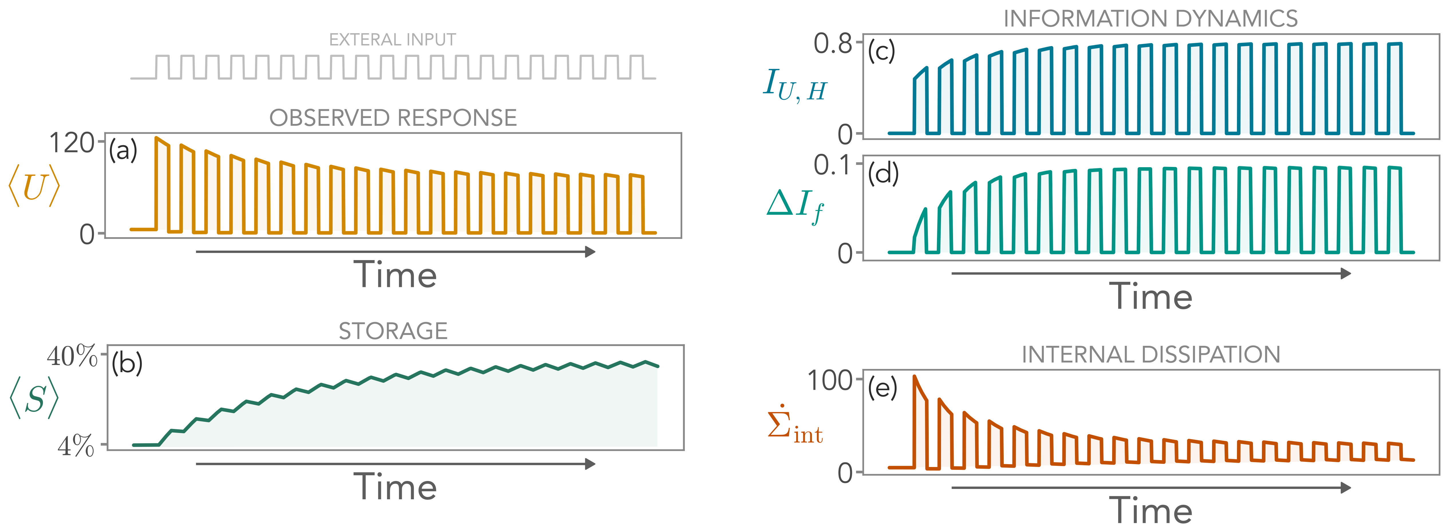
Figure 3: Evolution of the model at optimality under a switching external field $H(t)$. (a) The observed response is quantified by the average readout concentration $\expectationvalue{U}$ (orange) which decreases with the number of repetitions, adapting to the switching environment. For each time $t$, the fastest degrees of freedom reach a steady-state, hence the evolution of $\expectationvalue{U}$ cannot be interpreted as a relaxation dynamics. (b) Observed adaption can be seen as a consequence of the negative feedback from the storage population, whose average $\expectationvalue{S}$ (green) increases in time. At large times, the system reaches a periodic steady-state. (c) The information encoded on $H$ through the readout, $I_{U,H}$ (blue), increases in time during adaptation. (d) Simultaneously, adaptation also maximizes feedback information, $\Delta I_{f}$ (teal), indicating that the storage mechanism favors information in the system. (e) The dissipation rate to produce both readout and storage, $\dot{\Sigma}_{\rm int}$, decreases in time, highlighting the twofold information-thermodynamic advantage of adaptation. Model parameters in this figure are $\beta=2.5$, $\sigma=0.5$ (in the unit measure of the energy, for simplicity), and as specified in Appendix A.

III.1 Adaptation dynamically maximizes information and reduces internal dissipation

We have shown above that adaptive responses emerge in a narrow optimal region corresponding to a Pareto front that maximizes information and minimizes receptors dissipation. Although unexpected, this observation does not say anything about how relevant information-theoretic quantities dynamically behave during adaptation. To investigate this aspect and shed light on the information-thermodynamic advantages of adaptation, we now tune the parameters to the Pareto front, and study in detail the behavior of the system under a periodic switching signal.

In Figure 3a we show that, as expected, $\expectationvalue{U}$ decreases in time, adapting the response of the system to a repeated statistically identical input. This is a direct consequence of the increase of the average storage population, $\expectationvalue{S}$, which inhibits receptor activation (Figure 3b). We stress here that, due to the timescale separation regime, each point $\expectationvalue{U}(t)$ and $\expectationvalue{S}(t)$ plotted over time represents a steady-state of the system with respect to the fastest species, hence these dynamical features cannot be interpreted as a mere transient relaxation phenomenon. A mean-field relation between $\expectationvalue{U}$ and $\bar{\rho}_{S}=\expectationvalue{S}/N_{S}$ holds:

$$\frac{\langle U\rangle-\langle U\rangle_{r=1}}{\langle U\rangle_{r=1}-\langle U\rangle_{r=0}}=f_{0}(\bar{\rho}_{S})\;,$$ (8)

where $f_{0}(x)$ is a complex analytical function of its argument (see Supplementary Information), and $r=1(0)$ indicates that the receptor is active (passive). Eq. (8) allows us to consider only the percentage of storage molecules as the relevant parameter.

Figure 3c shows that the mutual information between $U$ and $H$, $I_{U,H}$, is not only in the optimal region, but it also increases in time. Although this result may seem surprising, we can understand it as a decrease in time of the Shannon entropy of the readout population due to repeated measurements of the signal. In fact,

$$\Delta\mathbb{S}_{U}=k_{B}\left(\mathcal{H}_{U|H}-\mathcal{H}_{U}\right)=-k_{B}I_{U,H}$$ (9)

where $\mathcal{H}_{X}$ is the Shannon entropy of $X$. This behavior is tightly related to the storage $S$, which acts as an information reservoir for the system. Indeed, if we consider that also $S$ contains information about the signal, we have that $\Delta\mathbb{S}_{U,S}<\Delta\mathbb{S}_{U}$ and thus the feedback information is positive, $\Delta I_{f}=I_{(U,S),H}-I_{U,H}>0$. Crucially, in the optimal region $\Delta I_{f}$ is maximized and increases in time as well (Figure 3d), signaling that adaptation amounts to a net gain of information when we consider both $U$ and $S$ together. See Supplementary Information for a detailed information-theoretic analysis.

These features come along with another intriguing result. When adaptation takes place, the concentrations of the internal species $U$ and $S$ change in time. It is therefore natural to ask how much energy is required to support these processes. We then introduce the rate of dissipation into the environment due to the internal mechanisms associated with the production of $U$ and $S$ (see Appendix D):

$$\dot{\Sigma}_{\rm int} = \sum_{u,s}\bigg{(}\Gamma_{s\to s+1}p_{U,S}(u,s,h,t)+$$

$$-\Gamma_{s+1\to s}p_{U,S}(u,s+1,h,t)\bigg{)}\log\frac{\Gamma_{s\to s+1}}{\Gamma_{s+1\to s}}$$

where $p_{U,S}$ is the joint probability distribution of $U$ and $S$ with all variables on which it depends written explicitly. We refer to $\dot{\Sigma}_{\rm int}$ as the internal dissipation of the system and, in Figure 3e, we show that it decreases in time during the adaptive response. This highlights a fundamental thermodynamic advantage of adaptation. After a large enough number of repetitions, the system has encoded the maximum amount of information on the environment and reaches a time-periodic steady-state, characterized by adapted readout and storage concentration. Such an adapted state lives close to the optimal parameter space in terms of information-dissipation trade-off. Additionally, the adaptive response that leads to this time-periodic state exhibits a dynamical maximization of all information features involving readout, storage, and external input increases, i.e., $I_{U,H}$ and $\Delta I_{f}$. As a synergistic effect, it also allows the system to tune the concentrations of internal species ($U$ and $S$) during its evolution so as to reduce the internal dissipation rate, $\dot{\Sigma}_{\rm int}$.

III.2 Information gain is optimal close to the information-dissipation trade-off

We have unraveled the intrinsic information-thermodynamic advantage of adaptive response emerging close to the optimal front. However, to understand how dynamical features such as information increase and dissipation reduction change with the model parameters, we need to characterize the response of the system in the whole $(\beta,\sigma)$ plane. For the sake of simplicity, we again focus on a large number of repetitions of a switching signal. To quantify the net increase in the encoded information, we introduce

$$\Delta I_{U,H}=I_{U,H}(t_{\rm st})-I_{U,H}(t_{1})$$ (11)

as the difference between $I_{U,H}$ after a signal at large times, $t_{\rm st}$, and the mutual information after the first signal, $t_{1}$ (see Supplementary Information for details about its estimation). The same quantity can be defined for the feedback information, $\Delta\Delta I_{f}$, and measures feedback efficacy. Analogously, $\Delta\dot{\Sigma}_{\rm int}$ quantifies the reduction of internal dissipation and, as such, it is expected to take negative values. Finally, the strength of adaptation is measured in terms of how much the average readout concentration decreases, i.e., $\Delta\expectationvalue{U}\leq 0$, where the equality holds only if adaptation is absent.

We find that the optimal front in the space of $\beta$ and $\sigma$ lies in the region in which adaption and feedback efficacies are both maximized (see Figure 4a-b). Therefore, dynamical features of information processing peak where the system is optimally responsive to a static field. Furthermore, the maximum of $\Delta I_{U,H}$ corresponds to intermediate values of adaptation, $\Delta\expectationvalue{U}$, and dissipation reduction, $\Delta\dot{\Sigma}_{\mathrm{int}}$. In fact, in a fixed range of $\beta$ we see in Figure 4c that, in principle, a strong adaptation may be reached for large values of $\sigma$, for which the internal dissipation is small as well. However, this corresponds to a loss of sensitivity to the external signal, as $\Delta I_{U,H}$ drastically decreases. The optimal surface corresponds both to intermediate values of $\Delta\expectationvalue{U}$ and $\Delta\dot{\Sigma}_{\mathrm{int}}$. Importantly, far away from the optimal front, we find either no reduction of dissipation during adaptation (top-right corner of Figures 4a-b) or detrimental feedback (lower dashed region of Figures 4a-b). These findings point to a deeper connection between the Pareto optimality highlighted in the previous analysis and the dynamical behavior of the system. In particular, the advantage in terms of information-processing capabilities during adaptation is dynamically optimal close to the region of parameters defined by the intrinsic information-dissipation trade-off.

Analyses of different signal and pause durations reveal a non-trivial interplay between the timescales of information storage and environmental dynamics. In particular, the more the system is exposed to the external signal, the more information it will store and use to adapt, up to the optimal encoding defined by the static picture (see Supplementary Information).

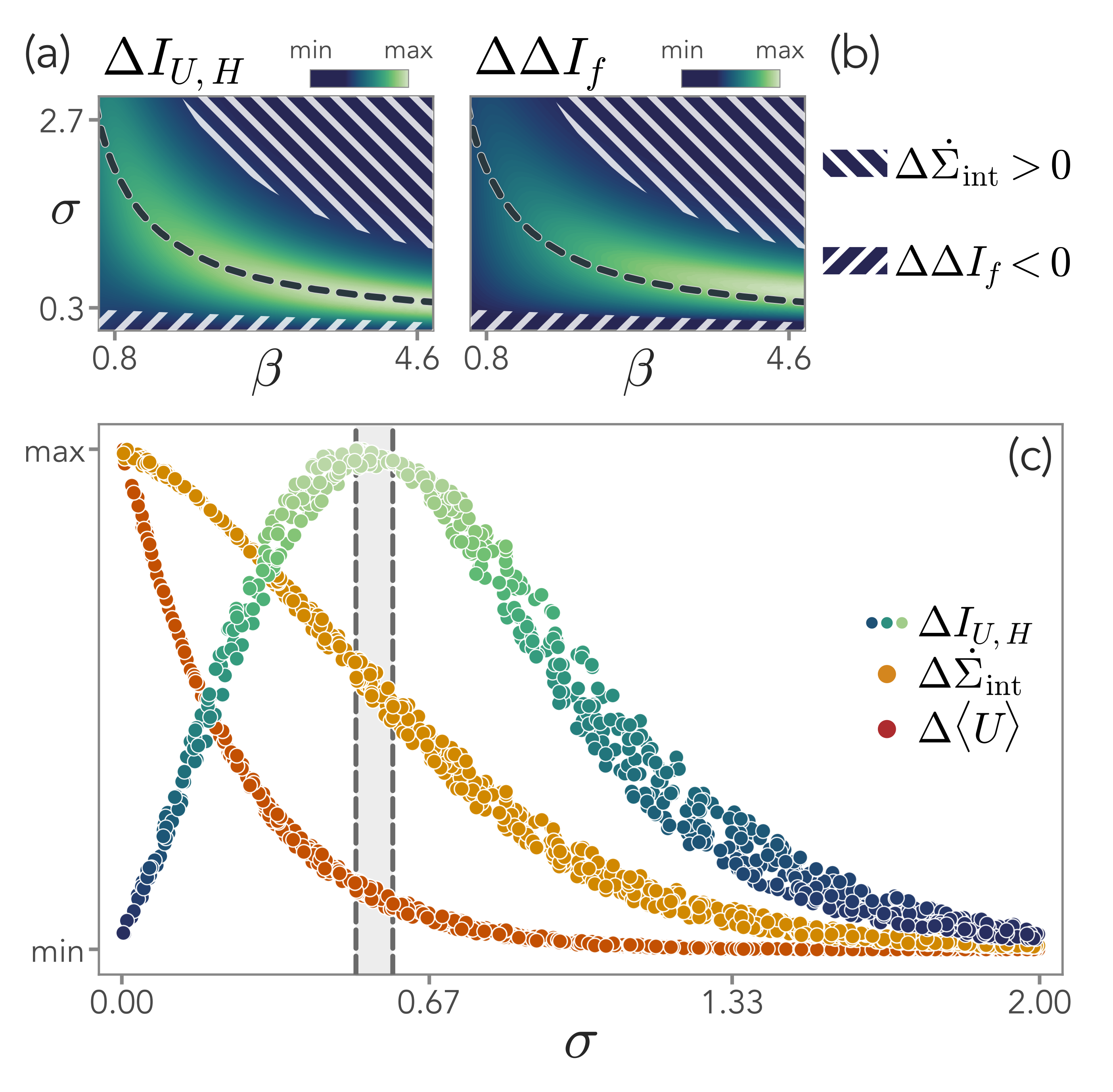
Figure 4: Optimality of information-gain close to the information-dissipation trade-off. (a) Contour plot of $\Delta I_{U,H}$ in the $(\beta,\sigma)$ plane. In the vicinity of the Pareto front (black dashed line), the information gained during the adaptive response is optimal. (b) The contour plot of $\Delta\Delta I_{f}$ in the $(\beta,\sigma)$ plane shows that the gain in the feedback information peaks around the Pareto front as well. Dashed regions in panels (a-b) indicate regions in which the feedback is ineffective during adaptation ($\Delta\Delta I_{f}<0$) and the internal dissipation increases upon repeated stimulation ($\Delta\dot{\Sigma}_{\rm int}>0$). These areas are far from the optimal Pareto front. (c) Projection of the contour plot along $\sigma$ for a range of values of $\beta\in[3-3.5]$ in the unit measure of the energy. The gray area enclosed by the dashed vertical lines indicates the location of the Pareto front for these values. $\Delta I_{U,H}$ clearly peaks at optimality, while $\Delta\expectationvalue{U}$ and $\Delta\dot{\Sigma}_{\rm int}$ take intermediate values.

IV The role of information storage

IV.1 A slow storage mechanism mediating feedback is necessary to drive adaptation

All the results obtained so far are connected to the proposed three-component archetypal model for sensing that encompasses a receptor, a readout, and a storage population. Therefore, one might ask whether the existence of a more minimal model, with a less complex structure, might lead to similar features. Here, we show that, in line with experimental and theoretical observations, the presence of a slow storage mechanism that mediates the negative feedback is crucial in driving adaptive responses in any biological system.

First, consider the case of negative feedback implemented directly by the readout $U$, bypassing the slower timescale in the network. As expected (and demonstrated in the Supplementary Information), since $U$ relaxes instantaneously, the feedback would be instantaneous as well. As a consequence, any modification of the concentration of $\expectationvalue{U}$ (the fastest component) will only affect its stationary distribution at each time $t$, excluding the emergence of any time-dependent effects. Since adaptation is intrinsically dynamic, it would be completely absent in this simplified model encompassing no storage mechanism. We can conclude that a slow mechanism, i.e., evolving on a timescale comparable to the external input, is needed to implement the negative feedback in a time-dependent fashion.

The second possibility to build a simpler two-component model, then, would reside in a slow readout population implementing once more direct negative feedback on the receptor. In this case, imagine to initialize the system with a low readout concentration (no signal). Then, the dynamics induced by a switching input would only be able to bring $\expectationvalue{U}$ to its steady-state, with intervals of growing (input on) and decreasing concentration (input off). As a result, $\expectationvalue{U}$ would qualitatively behave as $\expectationvalue{S}$ in Figure 3a, ruling out the presence of any adaptation mechanism in this simplified model. As a consequence, our model constitutes the minimal archetypal scheme for sensing, exhibiting a structure that is independent of the specific biological scale. Thus, the information-thermodynamic role of adaption must be a robust feature for any biological system operating close to optimality.

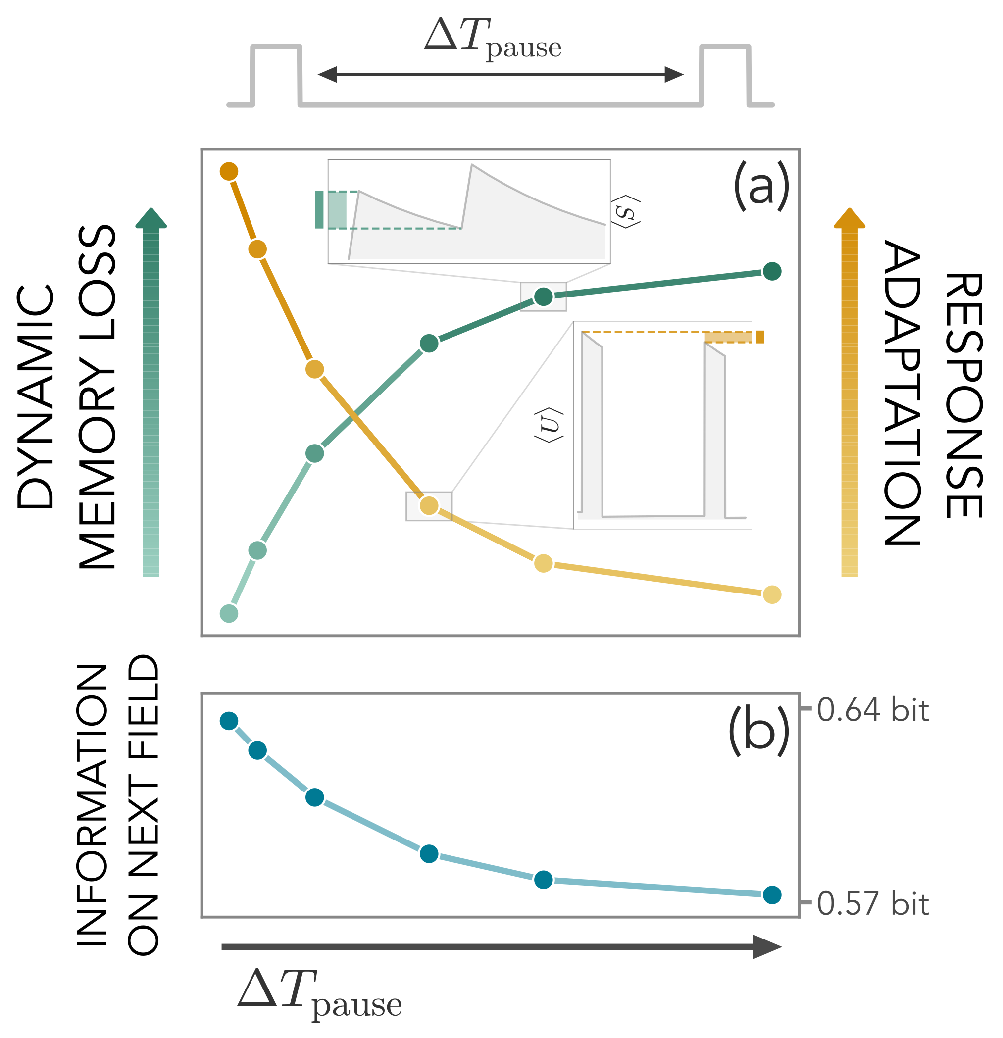
Figure 5: The role of memory in shaping adaptation. The system response depends on the waiting time $\Delta T_{\mathrm{pause}}$ between two external signals. As $\Delta T_{\mathrm{pause}}$ increases, the dynamical storage decays and thus memory is lost (green), whereas the adaptation of the readout population decreases (yellow). Insets show how dynamic memory loss and response adaptation are computed. (e) As a consequence, the information $I_{U,H}$ that the system has on the field $H$ when the new stimulus arrives decays as well. Model parameters for this figure are $\beta=2.5$, $\sigma=0.5$ in the unit measure of the energy, and as specified in Appendix A.

IV.2 An emergent finite-time memory

The proposed model is fully Markovian, despite clearly exhibiting a time-dependent behavior that depends on the timescales of the microscopic components. In other words, its dynamical features reveal the emergence of a finite-time memory, which governs readout adaptation and coincides with the storage relaxation timescale. In Figure 5a, we show that the more $\expectationvalue{S}$ relaxes between two consecutive signals, the less the readout population adapts to repeated stimuli. Such a concerted behavior ascribes to the storage population the role of an effective memory. As a consequence, the mutual information $I_{U,H}$ on the next field decreases as well, and the system needs to activate a larger number of $\expectationvalue{U}$ upon new stimulation (Figure 5b).

Remarkably, in the case of a chemical signaling network, this effect induced by $S$ can be indeed interpreted as a biochemical memory, and the storage population as a collection of molecules accountable for its implementation. In fact, all possible chemical architectures compatible with an adaptation dynamics present three different states, retracing the same building blocks of this model. This has been seen in simple computational models [48], olfactory sensory networks [42], molecular schemes governing cell cycle timing [41], and TNF signaling networks [12], to cite some examples. However, although a clear role and interpretation for each of these three components are often not easily accessible, our work may stimulate further quests in this direction, providing experimentally testable predictions on their relevance.

V Adaptation dynamics in the visual system of zebrafish larvae

Adaptation in neural systems is underscored by a decay in the neural responses upon repeated or sustained sensory stimulation. This is typically measured as a progressive reduction of the stimulus-driven neuronal firing rate [44, 45, 46]. While it is generally accepted and reported that inhibitory feedback mechanisms modulate the stimulus weight [49], in analogy to molecular negative feedback mechanisms, there are different theories about the actual functional role of adaptation in controlling the information flow, optimal processing, and sensitivity calibration [46]. However, the results shown so far highlight a clear information-thermodynamic advantage associated with the emergence of adaptive responses. To test whether our framework could capture the typical adaptation dynamics exhibited by the visual system of a living organism, we studied the response of zebrafish larvae to repeated stimulation. These widely used model organisms show from the early days of life a robust panel of sensory-driven behaviors, useful for linking neural circuits activity and motor outcomes [50]. We thus adopted an experimental paradigm based on volumetric multiphoton imaging [51]. We optically recorded the neuronal activity of $\approx 55000$ neurons across the whole brain in response to the repeated presentation of visual stimulation with a dark looming dot on a lighter background. In particular, we extract a subpopulation of $\approx 2400$ neurons with a temporal activity profile that is most correlated with the stimulation protocol (see Appendix E). Along with a reliable stimulus-evoked activity, the data showed a progressive decrease in response amplitudes, typical of a sensory adaptation process (Figure 6a-b). A 2-dimensional embedding of the activity profiles obtained via principal component analysis (PCA) clearly captures the adaptation dynamics (explained variance $\approx 70\%$). While the evolution of the evoked neural response is described by the first principal direction, adaptation is reflected in the second one (Figure 6e).

To adjust our model architecture to the mesoscopic scale of the visual system of zebrafish larvae, we identify each readout unit with a subpopulation of neurons. Crucially, we assume that neural activations are stochastic with a given probability (see Appendix E). These choices allow us to investigate the sole effects of the minimal mechanisms included in our framework, neglecting the specific features of local and global neural dynamics. The patterns of the model-generated raster plot are remarkably similar to those of the fluorescence signal (see Figure 6c-d). Moreover, a PCA of these simulated data reveals that, while the evoked neural response is replaced by the expected a switching dynamics, adaptation is once more fully captured along the second principal direction, closely resembling the experimental data (see Figure 6f). Notably, these results are qualitatively robust with respect to changes in the model parameters, as long as the system lives in the optimal Pareto front, i.e., minimizes receptor dissipation and maximizes readout information.

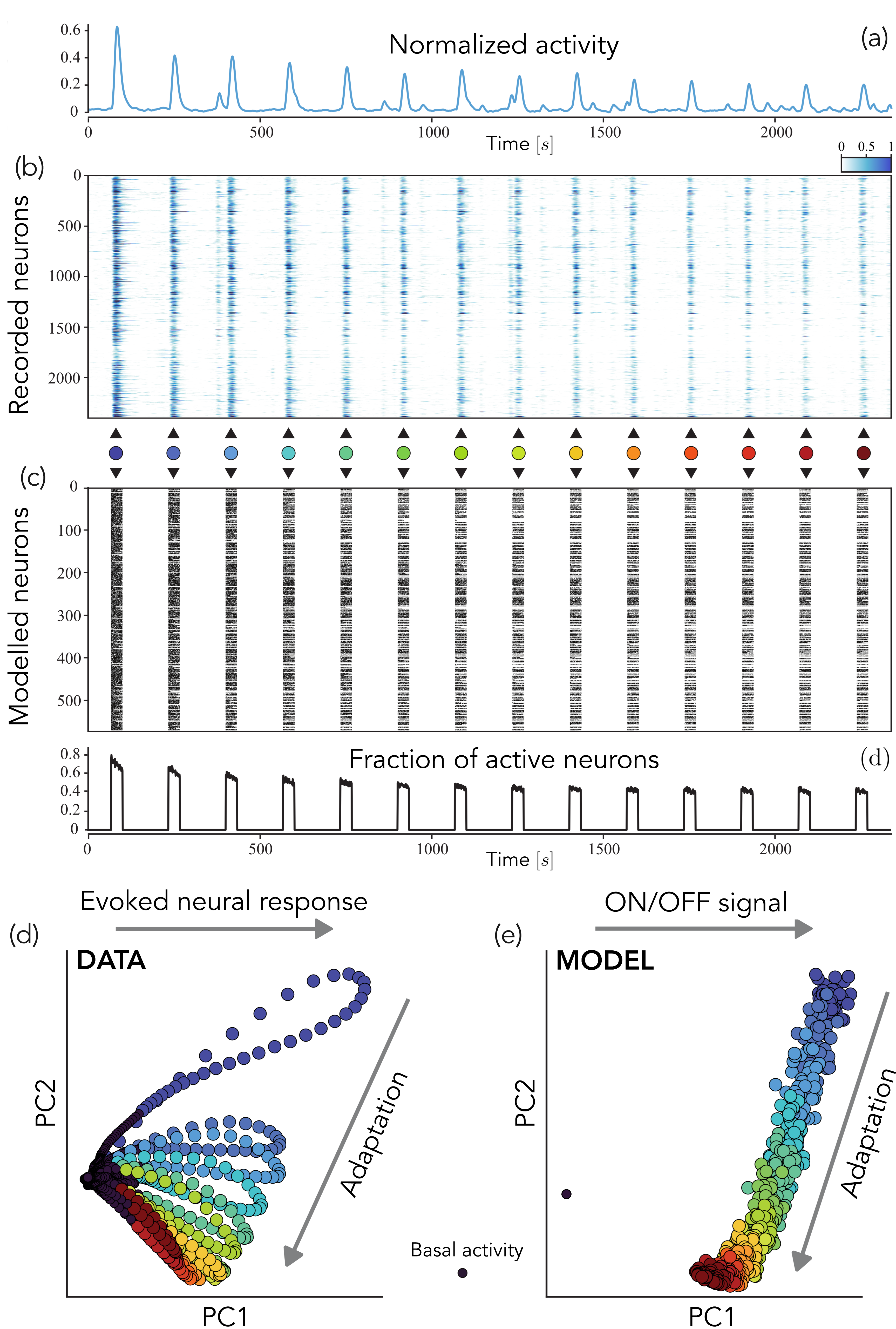
Figure 6: Adaptation dynamics in zebrafish larvae. (a-b) Normalized neural activity profile in a zebrafish larva in response to the repeated presentation of visual stimulation. Stimuli are indicated with colored dots from blue to red as time increases. (c) Raster plot of firing neurons at each time obtained from our model with stochastic neural activation. (d) Fraction of active neurons as a function of time. (e) PCA of experimental data reveals that adaptation is captured by the first two principal components. Adaptation is highlighted along the second principal direction, while features of the evoked neural response by the first one. Different colors indicate responses to different stimuli. (f) PCA of simulated neural activations. Although we do not model explicitly the evoked neural response, but rather an on/off switch of the signal, the core features of adaptation are correctly captured along the second principal direction. Model parameters are $\beta=3.5$, $\sigma=0.1$ in energy units, and as in Appendix A. Different parameters, provided that the model is close to the optimal region shown in Figure 2, do not qualitatively change the results.

This approach unravels the essential role of the minimal ingredients encoded in our model to explain the emergence of adaptation and its functional advantages. Indeed, we are able to capture the basic features of visual adaptation in zebrafish larvae without explicitly modeling the biological processes underlying neural dynamics. This suggests that the functional advantages of adaptation are rooted in the interplay between energy dissipation and information gain, although biological details remain crucial in shaping the evoked neural response and implementing these emerging features.

VI Summary and outlook

In this work, we introduce a minimal architecture that serves as an archetypal description of adaptation and information storage across biological scales, from biochemical networks to neural responses. It is informed by theoretical and experimental observations of different biological systems, and unravels the core mechanisms at the heart of adaptive behaviors. Starting with the natural requirement that any sensing mechanism has to maximize the information encoded on the environment, while minimizing the dissipation of the receptors, we find that adaptation spontaneously emerges at the Pareto front characterized by this information-dissipation trade-off. An analytical and numerical investigation of the dynamics of adaptive responses also reveals a clear twofold advantage of adaptation - reducing the dissipation of internal processes and simultaneously enhancing information processing capabilities. In fact, any adaptive system operating in the vicinity of the optimal front dynamically builds up information, optimizing the gain of both readout and storage populations.

Crucially, the resulting description can be consistently declined both for biochemical networks, where readout and storage populations have molecular counterparts, and more coarse-grained systems, where all ingredients have to be interpreted at a mesoscopic or macroscopic scale. As a proof of concept, we have employed it to describe sensory adaptation in the neural activity of a zebrafish larva exposed to repeated visual stimuli. Adaptive response is consistently captured without the need for biological details, hinting at the fact that dissipation, negative feedback, and information storage are minimal and necessary building blocks to describe any sensing mechanism. In particular, although here we studied sensory adaptation, it is reasonable to think that motor and, in general, behavioral adaptation [46] may stem from similar physical principles. Future works might unravel these aspects.

Extensions of these ideas are manifold. Although in the present work we focused on adaptation to repetitions of statistically identical signals, it will be interesting to characterize the system’s response to diverse environments [52]. To this end, incorporating multiple receptors and/or storage populations may be needed to harvest information in complex conditions. In such scenarios, correlations between external signals may help reduce the encoding effort. On a general ground, understanding how this encoded information is exploited by living systems is far more challenging and fascinating. For example, navigation in spatial environments, both in biological [53, 54] and bio-inspired artificial systems [55, 56], is an emergent behavior governed by how information about surroundings guides decision-making. Moreover, living systems do not passively read and adapt to external signals, but often act upon the environment. Adaptation dynamics and memory will remain core ingredients to model and grasp the complex information dynamics arising from this feedback mechanism. Further, understanding how information is used at the level of single agents will pave the way for the understanding of how collective intelligence emerges from the interaction of many information-processing units.

Our work serves as a fundamental framework for these ideas. Its main advantage is to provide a archetypal description of the necessary mechanisms to support information processing in a wide range of temporal and spatial scales, at the same time being minimal enough to allow for analytical treatments. As a consequence, we believe it may help the experimental quest for signatures of these physical ingredients in a variety of systems, many of which are only described at a phenomenological level. Ultimately, our results show how adaptation - a ubiquitous phenomenon that takes place at strikingly different biological scales - comes along with a thermodynamic and information-based advantage, explaining its relevance for any biological system.

Appendix A: Model parameters

The system is driven out of equilibrium by both the external field and the storage inhibition through the receptor dynamics, whose dissipation per unit temperature is $\delta Q_{R}$ (see Eq. (5)). The ratio $g=\Gamma^{0}_{H}/\Gamma^{0}_{I}$ sets the relative timescales of the two receptor pathways (see Eq. (1)). The energetic barrier $(V-cr)$ fixes the average values of the readout population both in the passive and active state, namely $\langle U\rangle_{P}=e^{-\beta V}$ and $\langle U\rangle_{A}=e^{-\beta(V-c)}$ (see Eq. (2)), and $\kappa$ controls the effectiveness of the storage in inhibiting the receptor’s activation. We assume that, on average, the activation rate due to the field is balanced by the feedback of a fraction $\alpha=\expectationvalue{S}/N_{S}$ of the storage population,

$$\expectationvalue{\log\frac{\Gamma_{P\to A}^{(H)}}{\Gamma_{A\to P}^{(I)}}}=\beta g\left(\expectationvalue{H}-\kappa\sigma\alpha\right)=0\quad\to\quad\kappa=\frac{\expectationvalue{H}}{\sigma\alpha},$$

so that we only need to fix $\alpha$. If not otherwise specified, we set $g=1$, i.e., $\Gamma^{0}_{H}=\Gamma^{0}_{I}\equiv\Gamma^{0}_{R}$, $\Delta E=1$, $\expectationvalue{U}_{A}=150$, $\expectationvalue{U}_{P}=0.5$, and $\alpha=2/3$. We remark that the emerging features of the model are independent of the specific choice of these parameters. Furthermore, we typically consider the average of the exponentially distributed signal to be $\langle H\rangle_{\mathrm{max}}=10$ and $\expectationvalue{H}_{\mathrm{min}}=0.1$ (see Supplementary Information).

Overall, we are left with $\beta$ and $\sigma$ as free parameters. $\beta$ quantifies the amount of thermal noise in the system, and at small $\beta$ the thermal activation of the receptor hinders the effect of the field and makes the system almost unable to process information. Conversely, if $\beta$ is high, the system must overcome large thermal inertia, increasing the dissipative cost. In this regime of weak thermal noise, we expect that, given a sufficient amount of energy, the system can effectively process information.

Appendix B: Model solution

1 Timescale separation procedure

We solve our system in a timescale separation framework [57, 58], where the storage evolves on a timescale that is much slower than all the other internal ones, i.e.,

$$\Gamma^{0}_{S}\ll\Gamma^{0}_{I}\approx\Gamma^{0}_{H}\ll\Gamma^{0}_{U}.$$

The fact that $\Gamma^{0}_{S}$ is the slowest timescale at play is crucial to make these components act as an information reservoir. This assumption is also compatible with biological examples. The main difficulty arises from the presence of the feedback, i.e. the field influences the receptor and thus the readout population, which in turn impacts the storage population and finally changes the chemical rate of the receptor - schematically, $H\to R\to U\to S\to R$. In order to solve the system, we need to properly take into account these effects.

We start with the master equation for the propagator $P(u,r,s,h,t|u_{0},r_{0},s_{0},h_{0},t_{0})$,

$$\partial_{t}P=\left[\frac{\hat{W}_{U}(r)}{\tau_{U}}+\frac{\hat{W}_{R}(s,h)}{\tau_{R}}+\frac{\hat{W}_{S}(u)}{\tau_{S}}+\frac{\hat{W}_{H}}{\tau_{H}}\right]P,$$

where $\tau_{U}\ll\tau_{R}\ll\tau_{S}\sim\tau_{H}$ are the timescales of the different processes, e.g., $\tau_{U}=1/\Gamma^{0}_{U}$. We rescale the time by $\tau_{S}$ and introduce two small parameters to control the timescale separation analysis, $\epsilon=\tau_{U}/\tau_{R}$ and $\delta=\tau_{R}/\tau_{H}$. Since $\tau_{S}/\tau_{H}=\mathcal{O}(1)$, we set it to $1$ without loss of generality. We then write $P=P^{(0)}+\epsilon P^{(1)}$ and expand the master equation to find $P^{(0)}=p^{\rm st}_{U|R}(u|r)\Pi$, with $\hat{W}_{U}\,p^{\rm st}_{U|R}=0$. Similarly, $\Pi$ obeys

$$\partial_{t}\Pi=\left[\delta^{-1}\hat{W}_{R}(s,h)+\hat{W}_{S}(u)+\hat{W}_{H}\right]\Pi.$$

Yet again, $\Pi=\Pi^{(0)}+\delta\Pi^{(1)}$ allows us to write $\Pi^{(0)}=p^{\rm st}_{R|S,H}(r|s,h)F(s,h,t|s_{0},h_{0},t_{0})$ at order $\mathcal{O}(\delta^{-1})$, where $\hat{W}_{R}\,p^{\rm st}_{R|S,H}=0$. Expanding first in $\epsilon$ and then in $\delta$ sets a hierarchy among timescales. Crucially, due to the feedback present in the system we cannot solve the next order explicitly to find $F$. Indeed, after a marginalization over $r$, we find $\partial_{t}F=\left[\hat{W}_{H}+\hat{W}_{S}\left(\bar{u}(s,h)\right)\right]F$, at order $\mathcal{O}(1)$, where $\bar{u}(s,h)=\sum_{u,r}u\,p^{\rm st}_{U|R}(u|r)p^{\rm st}_{R|S,H}(r|s,h)$. Hence, the evolution operator for $F$ depends manifestly on $s$, and the equation cannot be self-consistently solved. To tackle the problem, we first discretize time, considering a small interval, i.e., $t=t_{0}+\Delta t$ with $\Delta t\ll\tau_{U}$ and thus $\bar{u}(s,h)\approx u_{0}$. We thus find $F(s,h,t|s_{0},h_{0},t_{0})=P(s,t|s_{0},t_{0})P_{H}(h,t|h_{0},t_{0})$ in the domain $t\in[t_{0},t_{0}+\Delta t]$, since $H$ evolves independently from the system (see also Supplementary Information for analytical steps).

Iterating the procedure for multiple time steps, we end up with a recursive equation for the joint probability $p_{U,R,S,H}(u,r,s,h,t_{0}+\Delta t)$. We are interested in the following marginalization

$$p_{U,S}(u,t+\Delta t)= \sum_{r=0}^{1}\int_{0}^{\infty}dh\,p_{U|R}^{\rm st}(u|r)\,p_{R|S,H}^{\rm st}(r|h,s)\,p_{H}(h,t+\Delta t)\sum_{s^{\prime}=0}^{N_{S}}\sum_{u^{\prime}=0}^{\infty}P(s^{\prime},t\to s,t+\Delta t)|u^{\prime})p_{U,S}(u^{\prime},s^{\prime},t)$$ (1)

where $P(s^{\prime},t\to s,t+\Delta t)$ is the propagator of the storage at fixed readout. This is the Chapman-Kolmogorov equation in the timescale separation approximation. Notice that this solution requires the knowledge of $p_{U,S}$ at the previous time-step and it has to be solved iteratively.

2 Explicit solution for the storage propagator

To find a numerical solution to our system, we first need to compute the propagator $P(s_{0},t_{0}\to s,t)$. Formally, we have to solve the master equation

$$\partial_{t}P(s_{0}\to s|u_{0})=\Gamma^{0}_{S}\biggl{[} e^{-\beta\sigma}u_{0}P(s_{0}\to s^{\prime})\delta_{s^{\prime},s-1}+$$ (2)

$$+s^{\prime}P(s_{0}\to s^{\prime})\delta_{s^{\prime},s+1}+$$

$$-P(s_{0}\to s^{\prime})\delta_{s^{\prime},s}\left(s^{\prime}+e^{-\beta\sigma}u_{0}\right)\biggr{]}$$

where we used the shorthand notation $P(s_{0}\to s)=(s_{0},t_{0}\to s,t)$. Since our formula has to be iterated for small time-steps, i.e., $t-t_{0}=\Delta t\ll 1$, we can write the propagator as follows

$$P(s_{0},t_{0}\to s,t_{0}+\Delta t)|u_{0})=p_{S|U}^{\rm st}+\sum_{\nu}w_{\nu}a^{(\nu)}e^{\lambda_{\nu}\Delta t}$$ (3)

where $w_{\nu}$ and $\lambda_{\nu}$ are respectively eigenvectors and eigenvalues of the transition matrix $\hat{W}_{S}(u_{0})$,

$$\left(\hat{W}_{S}(u_{0})\right)_{ij} =e^{-\beta\sigma}u_{0}\quad i=j+1$$ if (4)

$$\left(\hat{W}_{S}(u_{0})\right)_{ij} =j\quad i=j-1$$ if

$$\left(\hat{W}_{S}(u_{0})\right)_{ij} =0\quad$$ otherwise

and the coefficients $a^{(\nu)}$ are such that

$$p_{S|U}(s_{0},t_{0}\to s,t_{0}+\Delta t)|u_{0})=p_{S|U}^{\rm st}+\sum_{\nu}w_{\nu}a^{(\nu)}=\delta_{s,s_{0}}.$$ (5)

Since eigenvalues and eigenvectors of $\hat{W}_{S}(u_{0})$ might be computationally expensive to find, we employ another simplification. As $\Delta t\to 0$, we can restrict the matrix only to jumps to the $n$-th nearest neighbors of the initial state $(s_{0},t_{0})$, assuming that all other states are left unchanged in small time intervals.

3 Computation of mutual information

Once we have $p_{U}(u,t)$ (obtained marginalizing $p_{U,S}$ over $s$) for a given $p_{H}(h,t)$, we can compute the mutual information

$$I_{U,H}(t)=\mathcal{S}[p_{U}](t)-\int_{0}^{\infty}dh\,p_{H}(h,t)\mathcal{S}[p_{U|H}](t)$$

where $\mathcal{S}$ is the Shannon entropy. For the sake of simplicity, we consider that the external field follows an exponential distribution $p_{H}(h,t)=\lambda(t)e^{-\lambda(t)h}$. Notice that, in order to determine such quantity, we need the conditional probability $p_{U|H}(u,t)$. In the Supplementary Information, we show how all the necessary joint and conditional probability distributions can be computed from the dynamical evolution derived above.

We also highlight here that the timescale separation implies $I_{S,H}=0$, since

$$p_{S|H}(s,t|h) =\sum_{u}p_{U,S|H}(u,s,t|h)$$

$$=p_{S}(s,t)\sum_{u}\sum_{r}p^{\rm st}_{U|R}(u|r)p^{\rm st}_{R|S,H}(r|s,h)$$

$$=p_{S}(s,t).$$

Although it may seem surprising, this is a direct consequence of the fact that $S$ is only influenced by $H$ through the stationary state of $U$. Crucially, the presence of the feedback is still fundamental to promote adaptation. Indeed, we can always write the mutual information between the field $H$ and both the readout $U$ and the storage $S$ together as $I_{(U,S),H}=\Delta I_{f}+I_{U,H}$, where $\Delta I_{f}=I_{(U,S),H}-I_{U,H}=I_{(U,H),S}-I_{U,S}$. Hence, if we have $\Delta I_{f}>0$ (as we shown in the main text), the storage is increasing the information of the two populations together on the external field. Overall, although $S$ and $H$ are independent in this limit, the feedback is paramount in shaping how the system responds to the external field and stores information about it.

Appendix C: Pareto optimization

We first perform a Pareto optimization at stationarity in the presence of a large, but static, external field. We seek the optimal values of $(\beta,\sigma)$ by maximizing the functional

$$\mathcal{L}(\beta,\sigma)= \gamma\frac{I_{U,H}(\beta,\sigma)}{\mathrm{max}(I_{U,H})}-(1-\gamma)\frac{\delta Q_{R}(\beta,\sigma)}{\mathrm{max}(\delta Q_{R})}$$ (6)

where $\gamma\in[0,1]$. Hence, we maximize the information between the readout and the field, simultaneously minimizing the dissipation of the receptor induced by both the signal and feedback process. The values are normalized since, in principle, they can span different orders of magnitudes. Later on, we find that the optimality of the information dynamics with a pulsating signal, in terms of adaptation and feedback efficacy, is attained for values of $\beta$ and $\sigma$ lying in the vicinity of this static Pareto-like front. In the Supplementary Information, we show that qualitatively similar results can be obtained for a $3$-d Pareto-like surface obtained by maximizing also the feedback information, $\Delta I_{f}$.

Appendix D: Dissipation of internal chemical processes

The production of readout, $u$, and storage, $s$, molecules requires energy. The dissipation into the environment can be quantified from the environmental contribution of the Schnakenberg entropy production, which is also the only one that survives at stationarity [59]. We have:

$$\dot{\Sigma}_{\rm int} = \sum_{u,s}\left(\Gamma_{u\to u+1}p_{U,S}(u,s,h,t)+\right.$$

$$\left.-\Gamma_{u+1\to u}p_{U,S}(u+1,s,h,t)\right)\log\frac{\Gamma_{u\to u+1}}{\Gamma_{u+1\to u}}+$$

$$+ \sum_{u,s}\left(\Gamma_{s\to s+1}p_{U,S}(u,s,h,t)+\right.$$

$$\left.-\Gamma_{s+1\to s}p_{U,S}(u,s+1,h,t)\right)\log\frac{\Gamma_{s\to s+1}}{\Gamma_{s+1\to s}}$$

where we indicated all possible dependencies in the joint probability distribution. By employing the timescale separation [57], and noting that $\Gamma_{u\to u\pm 1}$ do not depend on $s$, we finally have:

$$\dot{\Sigma}_{\rm int} = \sum_{u,s}\left(\Gamma_{s\to s+1}p_{U,S}(u,s,h,t)+\right.$$

$$\left.-\Gamma_{s+1\to s}p_{U,S}(u,s+1,h,t)\right)\log\frac{\Gamma_{s\to s+1}}{\Gamma_{s+1\to s}}$$

As this quantity decreases during adaptation, the system tends to dissipate less and less into the environment to produce the internal chemical populations that are required to encode and store the external signal.

Appendix E: Data and model of adaptation in zebrafish larve

1 Recording of whole brain neuronal activity in zebrafish larvae

Acquisitions of the zebrafish brain activity were carried out in Elavl3:H2BGCaMP6s larvae at 5 days post fertilization raised at $28^{\circ}C$ on a 12 h light/12 h dark cycle according to the approval by the Ethical Committee of the University of Padua (61/2020 dal Maschio). Larvae were embedded in 2 percent agarose gel and their brain activity was recorded using a multiphoton system with a custom 3D volumetric acquisition module. Data were acquired at 30 frames per second covering an effective field of view of about $450\times 900\mathrm{um}$ with a resolution of $512\times 1024$ pixels. The volumetric module acquires a volume of about $180-200\mathrm{um}$ in thickness encompassing $30$ planes separated by about $7\mathrm{um}$, at a rate of $1$ volume per second, sufficient to track the slow dynamics associated with the fluorescence-based activity reporter GCaMP6s. Visual stimulation was presented in the form of a looming stimulus with $150\mathrm{s}$ intervals, centered with the fish eye. See Supplementary Information.

2 Data analysis

The acquired temporal series were first processed using an automatic pipeline, including motion artifact correction, temporal filtering with a $3\mathrm{s}$ rectangular window, and automatic segmentation. The obtained dataset was manually curated to resolve segmentation errors or to integrate cells not detected automatically. We fit the activity profiles of about $55000$ cells with a linear regression model using a set of base functions representing the expected responses to each stimulation event. These base functions have been obtained by convolving the exponentially decaying kernel of the GCaMP signal lifetime with square waveforms characterizing the presentation of the corresponding visual stimulus. The resulting score coefficients of the fit were used to extract the cells whose score fell within the top $5\%$ of the distribution, resulting in a population of $\approx 2400$ neurons whose temporal activity profile correlates most with the stimulation protocol. The resulting fluorescence signals $F^{(i)}$ were processed by removing a moving baseline to account for baseline drifting and fast oscillatory noise [60]. See Supplementary Information.

3 Model for neural activity

Here, we describe how our framework is modified to mimic neural activity and reconstruct the raster plot in Figure 4. Each readout molecule is interpreted as a population of $N$ neurons, i.e., a region dedicated to the sensing of a specific input. Storage can be implemented in different ways, such as inhibitory neural populations or synaptic plasticity mechanisms, and we do not seek a detailed biological interpretation. When a readout population is activated at time $t$, each of its $N$ neurons fires with a probability $p$. We set $N=100$ and $p=0.5$, but changes in their values do not alter the results presented in the main text. In this way, at each time in which a readout unit is active, firing neurons are generally different even if we do not take into account the underlying neural dynamics. Due to adaptation, some of the readout units activated by the first stimulus will not be activated by subsequent stimuli. Although the evoked neural response cannot be captured by this extremely simple model, its archetypal ingredients (dissipation, storage, and feedback) are informative enough to reproduce the low-dimensional adaptation dynamics found in experimental data.

References

- Tkačik and Bialek [2016] G. Tkačik and W. Bialek, Information processing in living systems, Annual Review of Condensed Matter Physics 7, 89 (2016).
- Azeloglu and Iyengar [2015] E. U. Azeloglu and R. Iyengar, Signaling networks: information flow, computation, and decision making, Cold Spring Harbor perspectives in biology 7, a005934 (2015).
- Gnesotto et al. [2018] F. S. Gnesotto, F. Mura, J. Gladrow, and C. P. Broedersz, Broken detailed balance and non-equilibrium dynamics in living systems: a review, Reports on Progress in Physics 81, 066601 (2018).
- Nemenman [2012] I. Nemenman, Information theory and adaptation, Quantitative biology: from molecular to cellular systems 4, 73 (2012).
- Nakajima [2015] T. Nakajima, Biologically inspired information theory: Adaptation through construction of external reality models by living systems, Progress in Biophysics and Molecular Biology 119, 634 (2015).
- Whiteley et al. [2017] M. Whiteley, S. P. Diggle, and E. P. Greenberg, Progress in and promise of bacterial quorum sensing research, Nature 551, 313 (2017).
- Perkins and Swain [2009] T. J. Perkins and P. S. Swain, Strategies for cellular decision-making, Molecular systems biology 5, 326 (2009).
- Koshland Jr et al. [1982] D. E. Koshland Jr, A. Goldbeter, and J. B. Stock, Amplification and adaptation in regulatory and sensory systems, Science 217, 220 (1982).
- Tu et al. [2008] Y. Tu, T. S. Shimizu, and H. C. Berg, Modeling the chemotactic response of escherichia coli to time-varying stimuli, Proceedings of the National Academy of Sciences 105, 14855 (2008).
- Tu [2008] Y. Tu, The nonequilibrium mechanism for ultrasensitivity in a biological switch: Sensing by maxwell’s demons, Proceedings of the National Academy of Sciences 105, 11737 (2008).
- Mattingly et al. [2021] H. Mattingly, K. Kamino, B. Machta, and T. Emonet, Escherichia coli chemotaxis is information limited, Nature Physics 17, 1426 (2021).
- Cheong et al. [2011] R. Cheong, A. Rhee, C. J. Wang, I. Nemenman, and A. Levchenko, Information transduction capacity of noisy biochemical signaling networks, science 334, 354 (2011).
- Wajant et al. [2003] H. Wajant, K. Pfizenmaier, and P. Scheurich, Tumor necrosis factor signaling, Cell Death & Differentiation 10, 45 (2003).
- Lan et al. [2012] G. Lan, P. Sartori, S. Neumann, V. Sourjik, and Y. Tu, The energy–speed–accuracy trade-off in sensory adaptation, Nature physics 8, 422 (2012).
- Menini [1999] A. Menini, Calcium signalling and regulation in olfactory neurons, Current opinion in neurobiology 9, 419 (1999).
- Kohn [2007] A. Kohn, Visual adaptation: physiology, mechanisms, and functional benefits, Journal of neurophysiology 97, 3155 (2007).
- Lesica et al. [2007] N. A. Lesica, J. Jin, C. Weng, C.-I. Yeh, D. A. Butts, G. B. Stanley, and J.-M. Alonso, Adaptation to stimulus contrast and correlations during natural visual stimulation, Neuron 55, 479 (2007).
- Benucci et al. [2013] A. Benucci, A. B. Saleem, and M. Carandini, Adaptation maintains population homeostasis in primary visual cortex, Nature neuroscience 16, 724 (2013).
- Schneidman et al. [2006] E. Schneidman, M. J. Berry, R. Segev, and W. Bialek, Weak pairwise correlations imply strongly correlated network states in a neural population, Nature 440, 1007 (2006).
- Tkacik et al. [2014] G. Tkacik, O. Marre, D. Amodei, E. Schneidman, W. Bialek, and M. J. Berry, Searching for collective behavior in a large network of sensory neurons, PLoS computational biology 10, e1003408 (2014).
- Kurtz et al. [2015] Z. D. Kurtz, C. L. Müller, E. R. Miraldi, D. R. Littman, M. J. Blaser, and R. A. Bonneau, Sparse and compositionally robust inference of microbial ecological networks, PLoS computational biology 11, e1004226 (2015).
- Tunstrøm et al. [2013] K. Tunstrøm, Y. Katz, C. C. Ioannou, C. Huepe, M. J. Lutz, and I. D. Couzin, Collective states, multistability and transitional behavior in schooling fish, PLoS computational biology 9, e1002915 (2013).
- Nicoletti and Busiello [2021] G. Nicoletti and D. M. Busiello, Mutual information disentangles interactions from changing environments, Physical Review Letters 127, 228301 (2021).
- Nicoletti and Busiello [2022] G. Nicoletti and D. M. Busiello, Mutual information in changing environments: non-linear interactions, out-of-equilibrium systems, and continuously-varying diffusivities, Physical Review E 106, 014153 (2022).
- De Smet and Marchal [2010] R. De Smet and K. Marchal, Advantages and limitations of current network inference methods, Nature Reviews Microbiology 8, 717 (2010).
- Nicoletti et al. [2022] G. Nicoletti, A. Maritan, and D. M. Busiello, Information-driven transitions in projections of underdamped dynamics, Physical Review E 106, 014118 (2022).
- Celani et al. [2011] A. Celani, T. S. Shimizu, and M. Vergassola, Molecular and functional aspects of bacterial chemotaxis, Journal of Statistical Physics 144, 219 (2011).
- Kollmann et al. [2005] M. Kollmann, L. Løvdok, K. Bartholomé, J. Timmer, and V. Sourjik, Design principles of a bacterial signalling network, Nature 438, 504 (2005).
- de Ronde et al. [2010] W. H. de Ronde, F. Tostevin, and P. R. Ten Wolde, Effect of feedback on the fidelity of information transmission of time-varying signals, Physical Review E 82, 031914 (2010).
- Selimkhanov et al. [2014] J. Selimkhanov, B. Taylor, J. Yao, A. Pilko, J. Albeck, A. Hoffmann, L. Tsimring, and R. Wollman, Accurate information transmission through dynamic biochemical signaling networks, Science 346, 1370 (2014).
- Barkai and Leibler [1997] N. Barkai and S. Leibler, Robustness in simple biochemical networks, Nature 387, 913 (1997).
- Parrondo et al. [2015] J. M. Parrondo, J. M. Horowitz, and T. Sagawa, Thermodynamics of information, Nature physics 11, 131 (2015).
- Bennett [1982] C. H. Bennett, The thermodynamics of computation — a review, International Journal of Theoretical Physics 21, 905 (1982).
- Sagawa and Ueda [2009] T. Sagawa and M. Ueda, Minimal energy cost for thermodynamic information processing: measurement and information erasure, Physical review letters 102, 250602 (2009).
- Hartich et al. [2015] D. Hartich, A. C. Barato, and U. Seifert, Nonequilibrium sensing and its analogy to kinetic proofreading, New Journal of Physics 17, 055026 (2015).
- Skoge et al. [2013] M. Skoge, S. Naqvi, Y. Meir, and N. S. Wingreen, Chemical sensing by nonequilibrium cooperative receptors, Physical review letters 110, 248102 (2013).
- Lestas et al. [2010] I. Lestas, G. Vinnicombe, and J. Paulsson, Fundamental limits on the suppression of molecular fluctuations, Nature 467, 174 (2010).
- Coultrap and Bayer [2012] S. J. Coultrap and K. U. Bayer, Camkii regulation in information processing and storage, Trends in neurosciences 35, 607 (2012).
- Frankland and Josselyn [2016] P. W. Frankland and S. A. Josselyn, In search of the memory molecule, Nature 535, 41 (2016).
- Lisman et al. [2002] J. Lisman, H. Schulman, and H. Cline, The molecular basis of camkii function in synaptic and behavioural memory, Nature Reviews Neuroscience 3, 175 (2002).
- Rahi et al. [2017] S. J. Rahi, J. Larsch, K. Pecani, A. Y. Katsov, N. Mansouri, K. Tsaneva-Atanasova, E. D. Sontag, and F. R. Cross, Oscillatory stimuli differentiate adapting circuit topologies, Nature methods 14, 1010 (2017).
- Tadres et al. [2022] D. Tadres, P. H. Wong, T. To, J. Moehlis, and M. Louis, Depolarization block in olfactory sensory neurons expands the dimensionality of odor encoding, Science Advances 8, eade7209 (2022).
- Jalaal et al. [2020] M. Jalaal, N. Schramma, A. Dode, H. de Maleprade, C. Raufaste, and R. E. Goldstein, Stress-induced dinoflagellate bioluminescence at the single cell level, Physical Review Letters 125, 028102 (2020).
- Malmierca et al. [2014] M. S. Malmierca, M. V. Sanchez-Vives, C. Escera, and A. Bendixen, Neuronal adaptation, novelty detection and regularity encoding in audition, Frontiers in Systems Neuroscience 8, 10.3389/fnsys.2014.00111 (2014).
- Shew et al. [2015] W. L. Shew, W. P. Clawson, J. Pobst, Y. Karimipanah, N. C. Wright, and R. Wessel, Adaptation to sensory input tunes visual cortex to criticality, Nature Physics 11, 659 (2015).
- Benda [2021] J. Benda, Neural adaptation, Current Biology 31, R110 (2021).
- Ngampruetikorn et al. [2020] V. Ngampruetikorn, D. J. Schwab, and G. J. Stephens, Energy consumption and cooperation for optimal sensing, Nature communications 11, 1 (2020).
- Ma et al. [2009] W. Ma, A. Trusina, H. El-Samad, W. A. Lim, and C. Tang, Defining network topologies that can achieve biochemical adaptation, Cell 138, 760 (2009).
- Lamiré et al. [2022] L.-A. Lamiré, M. Haesemeyer, F. Engert, M. Granato, and O. Randlett, Inhibition drives habituation of a larval zebrafish visual response, bioRxiv , 2022 (2022).
- Dal Maschio et al. [2017] M. Dal Maschio, J. C. Donovan, T. O. Helmbrecht, and H. Baier, Linking neurons to network function and behavior by two-photon holographic optogenetics and volumetric imaging, Neuron 94, 774 (2017).
- Bruzzone et al. [2021] M. Bruzzone, E. Chiarello, M. Albanesi, M. E. Miletto Petrazzini, A. Megighian, C. Lodovichi, and M. Dal Maschio, Whole brain functional recordings at cellular resolution in zebrafish larvae with 3d scanning multiphoton microscopy, Scientific reports 11, 11048 (2021).
- Hidalgo et al. [2014] J. Hidalgo, J. Grilli, S. Suweis, M. A. Munoz, J. R. Banavar, and A. Maritan, Information-based fitness and the emergence of criticality in living systems, Proceedings of the National Academy of Sciences 111, 10095 (2014).
- Tu [2013] Y. Tu, Quantitative modeling of bacterial chemotaxis: signal amplification and accurate adaptation, Annual review of biophysics 42, 337 (2013).
- Carrara et al. [2021] F. Carrara, A. Sengupta, L. Behrendt, A. Vardi, and R. Stocker, Bistability in oxidative stress response determines the migration behavior of phytoplankton in turbulence, Proceedings of the National Academy of Sciences 118, e2005944118 (2021).
- Liebchen and Löwen [2018] B. Liebchen and H. Löwen, Synthetic chemotaxis and collective behavior in active matter, Accounts of chemical research 51, 2982 (2018).
- Marchetti et al. [2013] M. C. Marchetti, J.-F. Joanny, S. Ramaswamy, T. B. Liverpool, J. Prost, M. Rao, and R. A. Simha, Hydrodynamics of soft active matter, Reviews of modern physics 85, 1143 (2013).
- Busiello et al. [2020] D. M. Busiello, D. Gupta, and A. Maritan, Coarse-grained entropy production with multiple reservoirs: Unraveling the role of time scales and detailed balance in biology-inspired systems, Physical Review Research 2, 043257 (2020).
- Bo and Celani [2017] S. Bo and A. Celani, Multiple-scale stochastic processes: decimation, averaging and beyond, Physics reports 670, 1 (2017).
- Schnakenberg [1976] J. Schnakenberg, Network theory of microscopic and macroscopic behavior of master equation systems, Reviews of Modern physics 48, 571 (1976).
- Jia et al. [2011] H. Jia, N. L. Rochefort, X. Chen, and A. Konnerth, In vivo two-photon imaging of sensory-evoked dendritic calcium signals in cortical neurons, Nature protocols 6, 28 (2011).