SAN: Inducing Metrizability of GAN with
Discriminative Normalized Linear Layer

Abstract

Generative adversarial networks (GANs) learn a target probability distribution by optimizing a generator and a discriminator with minimax objectives. This paper addresses the question of whether such optimization actually provides the generator with gradients that make its distribution close to the target distribution. We derive metrizable conditions, sufficient conditions for the discriminator to serve as the distance between the distributions by connecting the GAN formulation with the concept of sliced optimal transport. Furthermore, by leveraging these theoretical results, we propose a novel GAN training scheme, called slicing adversarial network (SAN). With only simple modifications, a broad class of existing GANs can be converted to SANs. Experiments on synthetic and image datasets support our theoretical results and the SAN’s effectiveness as compared to usual GANs. Furthermore, we also apply SAN to StyleGAN-XL, which leads to state-of-the-art FID score amongst GANs for class conditional generation on ImageNet 256$\times$256.

1 Introduction

A generative adversarial network (GAN) (Goodfellow et al., 2014) is a popular approach for generative modeling. GANs have achieved remarkable performance in various domains such as image (Brock et al., 2019; Karras et al., 2019; 2021), audio (Kumar et al., 2019; Donahue et al., 2019; Kong et al., 2020), and video (Tulyakov et al., 2018; Hao et al., 2021). The aim of GAN is to learn a target probability measure via a neural network, called a generator. To achieve this, a discriminator is introduced, and the generator and discriminator are optimized in a minimax way.

Here, we pose the question of whether GAN optimization actually makes the generator distribution close to the target distribution. For example, likelihood-based generative models such as variational autoencoders (Kingma & Welling, 2014; Higgins et al., 2017; Zhao et al., 2019; Takida et al., 2022), normalizing flows (Tabak & Vanden-Eijnden, 2010; Tabak & Turner, 2013; Rezende & Mohamed, 2015), and denoising diffusion probabilistic models (Ho et al., 2020; Song et al., 2020; Nichol & Dhariwal, 2021) are optimized via the principle of minimizing the exact Kullback–Leibler divergence or its upper bound (Jordan et al., 1999). For GANs, in contrast, it is known that solving the minimization problem with the optimal discriminator is equivalent to minimizing a specific dissimilarity (Goodfellow et al., 2014; Nowozin et al., 2016; Lim & Ye, 2017; Miyato et al., 2018). Furthermore, GANs have been analyzed on the basis of the optimal discriminator assumption (Chu et al., 2020). However, real-world GAN optimizations hardly achieve maximization (Fiez et al., 2022), and analysis of GAN optimization without that assumption is still challenging.

To analyze and investigate GAN optimization without the optimality assumption, there are approaches from the perspectives of training convergence (Mescheder et al., 2017; Nagarajan & Kolter, 2017; Mescheder et al., 2018; Sanjabi et al., 2018; Xu et al., 2020), loss landscape around the saddle points of minimax problems (Farnia & Ozdaglar, 2020; Berard et al., 2020), and the smoothness of optimization (Fiez et al., 2022). Although these studies have been insightful for GAN stabilization, there has been little discussion on whether trained discriminators indeed provide generator optimization with gradients that reduce dissimilarities.

Table 1: Common GAN losses do not simultaneously satisfy all the sufficient conditions given in Theorem 5.3. Thus, we propose the SAN to address one of the conditions, direction optimality. Even if a direction $\omega$ is the maximizer of the inner problems ${\mathcal{V}}$, it does not satisfy direction optimality except in Wasserstein GAN (see Sec. 6). The results in Appx. E empirically demonstrate that a discriminator trained on Wasserstein GAN tends not to satisfy separability. The last condition of injectivity depends on the discriminator implementation (see Appx. E for empirical verification).

	Direction optimality	Separability	Injectivity
Wassertein GAN	✓	weak	$\ast$
GAN (Hinge, Saturating, Non-saturating)	✗	✓	$\ast$
SAN (Hinge, Saturating, Non-saturating)	✓	✓	$\ast$

In this paper, we provide a novel perspective on GAN optimization, which helps us to consider whether a discriminator is metrizable.

Definition 1.1 (Metrizable discriminator).

Let $\mu_{\theta}$ and $\mu_{0}$ be measures. Given an objective function ${\mathcal{J}}(\theta;\cdot)$ for $\theta$, a discriminator $f$ is $({\mathcal{J}},{\mathcal{D}})$- or ${\mathcal{J}}$-metrizable for $\mu_{\theta}$ and $\mu_{0}$, if ${\mathcal{J}}(\theta;f)$ is minimized only with $\theta\in\mathrm{arg~{}min}_{\theta}{\mathcal{D}}(\mu_{0},\mu_{\theta})$ for a certain distance on measures, ${\mathcal{D}}(\cdot,\cdot)$.

To evaluate the dissimilarity with a given GAN minimization problem ${\mathcal{J}}$, we are interested in other conditions besides the discriminator’s optimality. Hence, we propose metrizable conditions, namely, direction optimality, separability, and injectivity, that induce ${\mathcal{J}}$-metrizable discriminator. To achieve this, we first introduce a divergence, called functional mean divergence (FM^∗), in Sec. 3. We connect the FM^∗ with the minimization objective function of Wasserstein GAN. Then, we obtain the metrizable conditions for Wasserstein GAN by investigating Question 1.2. We provide an answer to this question in Sec. 4 by relating the FM^∗ to the concept of sliced optimal transport (Bonneel et al., 2015; Kolouri et al., 2019). Then, in Sec. 5, we formalize the proposed conditions for Wasserstein GAN and further extend the result to generic GAN.

Question 1.2.

Under what conditions is FM^∗ a distance?

Based on the derived metrizable conditions, we propose the Slicing Adversarial Network (SAN) in Sec. 6. As seen in Table 1, we find that optimal discriminators for most existing GANs do not satisfy direction optimality. Hence, we develop a modification scheme for GAN maximization problems to enforce direction optimality on our discriminator. Owing to the scheme’s simplicity, GANs can easily be converted to SANs. We conduct experiments to verify our perspective and demonstrate that SANs are superior to GANs in certain generation tasks on synthetic and image datasets. In particular, we confirmed a SAN improves state-of-the-art FID for conditional generation with StyleGAN-XL (Sauer et al., 2022) on ImageNet 256$\times$256 despite the simple modifications.

2 Preliminaries

2.1 Notations

We consider a sample space $X\subseteq\mathbb{R}^{D_{x}}$ and a latent space $Z\subseteq\mathbb{R}^{D_{z}}$. Let ${\mathcal{P}}(X)$ be the set of all probability measures on $X$, and let $L^{\infty}(X,{\mathbb{R}}^{D})$ denote the $L^{\infty}$ space for functions $X\mapsto{\mathbb{R}}^{D}$. Let $\mu$ (or $\nu$) represent a probability measure with probability density function $I_{\mu}$ (or $I_{\nu}$). Denote $d_{h}(\mu,\nu):=\mathbb{E}_{x\sim\mu}[h(x)]-\mathbb{E}_{x\sim\nu}[h(x)]$. We use the notation of the pushforward operator $\sharp$, which is defined as $g_{\sharp}\sigma:=\sigma(g^{-1}(B))$ for $B\in X$ with a function $g:Z\to X$ and a probability measure $\sigma\in{\mathcal{P}}(Z)$. We denote the Euclidean inner product by $\langle\cdot,\cdot\rangle$. Lastly, $\hat{(\cdot)}$ denotes a normalized vector.

2.2 Problem Formulation in GANs

Assume that we have data obtained by discrete sampling from a target probability distribution $\mu_{0}\in{\mathcal{P}}(X)$. Then, we introduce a trainable generator function $g_{\theta}:Z\to{X}$ with parameter $\theta\in{\mathbb{R}}^{D_{\theta}}$ to model a trainable probability measure as $\mu_{\theta}=g_{\theta\sharp}\sigma$ with $\sigma\in{\mathcal{P}}(Z)$ The aim of generative modeling here is to learn $g_{\theta}$ so that it approximates the target measure as $\mu_{\theta}\approx\mu_{0}$.

For generative modeling in GAN, we introduce the notion of a discriminator $f\in{\mathcal{F}}(X)\subset L^{\infty}(X,{\mathbb{R}})$. We formulate the GAN’s optimization problem as a two-player game between the generator and discriminator with ${\mathcal{V}}:{\mathcal{F}}(X)\times{\mathcal{P}}(X)\to{\mathbb{R}}$ and ${\mathcal{J}}:{\mathbb{R}}^{D_{\theta}}\times{\mathcal{F}}(X)\to{\mathbb{R}}$, as follows:

$$\max_{f\in{\mathcal{F}}(X)}{\color[rgb]{0,0,0}{{{\mathcal{V}}(f;\mu_{\theta})}}}\quad\text{and}\quad\min_{\theta\in{\mathbb{R}}^{D_{\theta}}}{\mathcal{J}}(\theta;f).$$ (1)

Regarding the choices of ${\mathcal{V}}$ and ${\mathcal{J}}$, there are GAN variants (Goodfellow et al., 2014; Nowozin et al., 2016; Arjovsky et al., 2017) that lead to different dissimilarities between $\mu_{0}$ and $\mu_{\theta}$ with the maximizer $f$. In this paper, we use a representation of the discriminator in an inner-product form

$$f(x)=\langle\omega,h(x)\rangle,$$ (2)

where $\omega\in{\mathbb{S}}^{D-1}$ and $h(x)\in L(X,{\mathbb{R}}^{D})$. The form is naturally represented by a neural network.

2.3 Wasserstein Distance and Its Use for GANs

We consider the Wasserstein-$p$ distance (Villani, 2009) between probability measures $\mu$ and $\nu$

$$\textit{W}_{p}(\mu,\nu):=\left(\inf_{\pi\in\Pi(\mu,\nu)}\int_{{X}\times{X}}\|x-x^{\prime}\|_{p}^{p}d\pi(x,x^{\prime})\right)^{\frac{1}{p}},$$ (3)

where $p\in[1,\infty)$ and $\Pi(\mu,\nu)$ is the set of all coupling measures whose marginal distributions are $\mu$ and $\nu$. The idea of Wasserstein GAN is to learn a generator by minimizing the Wasserstein-1 distance between $\mu_{0}$ and $\mu_{\theta}$. For this goal, one can adopt the Kantorovich–-Rubinstein (KR) duality representation to rewrite Eq. (3) and obtain the following optimization problem:

$$\max_{f\in{\mathcal{F}}_{\text{Lip}}(X)}{\mathcal{V}}_{\text{Wass}}(f;\mu_{\theta}):=d_{f}(\mu_{0},\mu_{\theta})$$ (4)

where ${\mathcal{F}}_{\text{Lip}}$ denotes the class of 1-Lipschitz functions. In contrast, we formulate an optimization problem for the generator as minimization of the right side of Eq. (4) w.r.t. the generator parameter:

$${\color[rgb]{0,0,0}{{\min_{\theta\in\mathbb{R}^{D_{\theta}}}{\mathcal{J}}_{\text{Wass}}(\theta;f):=-\mathbb{E}_{x\sim\mu_{\theta}}[f(x)].}}}$$ (5)

2.4 Sliced Optimal Transport

The Wasserstein distance is highly intractable when the dimension $D_{x}$ is large (Arjovsky et al., 2017). However, it is well known that sliced optimal transport can be applied to break this intractability, by projecting the data on a one-dimensional space. That is, for the $D_{x}=1$ case, the Wasserstein distance has a closed-form solution:

$$\textit{W}_{p}(\mu,\nu)=\left(\int_{0}^{1}|F^{-1}_{\mu}(\rho)-F^{-1}_{\nu}(\rho)|^{p}d\rho\right),$$ (6)

where $F^{-1}_{\mu}(\cdot)$ denotes the quantile function for $I_{\mu}$. The closed-form solution for a one-dimensional space prompted the emergence of the concept of sliced optimal transport.

In the original sliced Wasserstein distance (SW) (Bonneel et al., 2015), a probability density function $I$ on the data space $X$ is mapped to a probability density function of $\xi\in{\mathbb{R}}$ by the standard Radon transform (Natterer, 2001; Helgason, 2011) as ${\mathcal{R}}{I}(\xi,\omega):=\int_{{X}}I(x)\delta(\xi-\langle x,\omega\rangle)dx$, where $\delta(\cdot)$ is the Dirac delta function and $\omega\in{\mathbb{S}}^{D_{x}-1}$ is a direction. The sliced Wasserstein distance between $\mu$ and $\nu$ is defined as $\textit{SW}_{p}^{h,\omega}(\mu,\nu):=(\int_{\omega\in{\mathbb{S}}^{D_{x}-1}}\textit{W}_{p}^{p}({\mathcal{R}}{I}_{\mu}(\cdot,\omega),{\mathcal{R}}{I_{\nu}}(\cdot,\omega))d\omega)^{1/p}$. Intuitively, the idea behind this distance is to decompose high-dimensional distributions into an infinite number of pairs of tractable distributions by linear projections.

Various extensions of the sliced Wasserstein distance have been proposed (Kolouri et al., 2019; Deshpande et al., 2019; Nguyen et al., 2021). Here, we review an extension called augmented sliced Wasserstein distance (ASW) (Chen et al., 2022). Given a measurable injective function $h:X\to{\mathbb{R}}^{D}$, the distance is obtained via the spatial Radon transform (SRT), which is defined for any $\xi\in{\mathbb{R}}$ and $\omega\in{\mathbb{S}}^{d-1}$, as follows:

$${\mathcal{S}}^{h}{I}(\xi,\omega):=\int_{{X}}I(x)\delta(\xi-\langle\omega,h(x)\rangle)dx.$$ (7)

The ASW-$p$ is then obtained via the SRT in the same fashion as the standard SW:

$$\textit{ASW}_{p}^{h}(\mu,\nu):=\left(\int_{\omega\in{\mathbb{S}}^{d-1}}\!\!\!\!\!\textit{W}_{p}^{p}({\mathcal{S}}^{h}{I}_{\mu}(\cdot,\omega),{\mathcal{S}}^{h}{I_{\nu}}(\cdot,\omega))d\omega\right)^{\frac{1}{p}}\!\!\!.$$ (8)

Equation (6) can be used to evaluate the integrand in Eq. (8), which is usually evaluated via approximated quantile functions with sorted finite samples from ${\mathcal{S}}^{h}{I_{\nu}}(\cdot,\omega)$ and ${\mathcal{S}}^{h}{I_{\nu}}(\cdot,\omega)$.

3 Formulation of Question 1.2

Next, we introduce a divergence, the functional mean divergence, FM or FM^∗, which is defined for a given functional space or function. Minimization of the FM^∗ can be formulated as an optimization problem involving ${\mathcal{J}}_{\text{Wass}}$, and we cast Question 1.2 in this context. In Sec. 4, we provide an answer to that question, which in turn provides the metrizable conditions with ${\mathcal{J}}_{\text{Wass}}$ in Sec. 5.

3.1 Proposed Framework: Functional Mean Divergence

We start by defining the FM with a given functional space.

Definition 3.1 (Functional Mean Divergence (FM)).

We define a family of FMs as

$$\mathscr{D}^{\text{FM}}_{D}:=\left\{(\mu,\nu)\mapsto\max_{h\in{\mathcal{F}}(X)}\left\|d_{h}(\mu,\nu)\right\|_{2}|{\mathcal{F}}(X)\subseteq L^{\infty}(X,{\mathbb{R}}^{D})\right\},$$ (9)

Further, we denote an instance in the family as $\textit{FM}_{{\mathcal{F}}}(\mu,\nu)\in\mathscr{D}^{\text{FM}}_{D}$, where ${\mathcal{F}}(X)\subseteq L^{\infty}(X,{\mathbb{R}}^{D})$.

By definition, the FM family includes the integral probability metric (IPM) (Müller, 1997), which includes the Wasserstein distance in KR form as a special case.

Proposition 3.2.

For ${\mathcal{F}}(X)\in L^{\infty}(X,{\mathbb{R}})$, $\textit{IPM}_{{\mathcal{F}}}(\cdot,\cdot):=\max_{f\in{\mathcal{F}}}d_{f}(\cdot,\cdot)\in\mathscr{D}^{\text{FM}}_{1}$.

The FM is an extension of the IPM to deal with vector-valued functional spaces. Although the FM with a properly selected functional space yields a distance between target distributions, the maximization in Eq. (9) is generally hard to achieve. Instead, we use the following metric, which is defined for a given function.

Definition 3.3 (Functional Mean Divergence^∗ (FM^∗)).

Given a functional space ${\mathcal{F}}(X)\subseteq L^{\infty}(X,{\mathbb{R}}^{D})$, we define a family of FMs^∗ as

$$\mathscr{D}^{\text{FM*}}_{{\mathcal{F}}}:=\left\{(\mu,\nu)\mapsto\|d_{h}(\mu,\nu)\|_{2}|h\in{\mathcal{F}}(X)\right\},$$ (10)

Further, we denote an instance in the family as $\textit{FM}_{h}^{*}(\mu,\nu)\in\mathscr{D}^{\text{FM*}}_{{\mathcal{F}}}$, where $h\in{\mathcal{F}}(X)$.

We are interested in Question 3.4, which is a mathematical formulation of Question 1.2. We give an answer to this question in Sec. 4. Because optimization of the FM^∗ is related to ${\mathcal{J}}_{\text{Wass}}$ in Sec. 3.2, the conditions in Question 3.4 enable us to derive $({\mathcal{J}}_{\text{Wass}},\textit{FM}_{h}^{*})$-metrizable conditions in Sec. 5.

Question 3.4.

Under what conditions for ${{\mathcal{F}}}(X)\in L^{\infty}(X,{\mathbb{R}}^{D})$ are $\textit{FM}_{h}^{*}(\cdot,\cdot)\in\mathscr{D}^{\text{FM*}}_{{\mathcal{F}}}$ distances?

3.2 Direction Optimality to Connect FM^∗ and ${\mathcal{J}}_{\text{Wass}}$

Optimization of the FM^∗ with a given $h\in L^{\infty}(X,{\mathbb{R}}^{D})$ returns us to an optimization problem involving ${\mathcal{J}}_{\text{Wass}}$.

Proposition 3.5 (Direction optimality connects FM^∗ and ${\mathcal{J}}_{\text{Wass}}$).

Let $\omega$ be on ${\mathbb{S}}^{D-1}$. For any $h\in L^{\infty}(X,{\mathbb{R}}^{D})$, minimization of $\textit{FM}_{h}^{*}(\mu_{\theta},\mu_{0})$ is equivalent to optimization of $\min_{\theta\in{\mathbb{R}}^{D_{\theta}}}\max_{\omega\in{\mathbb{S}}^{D-1}}{\mathcal{J}}_{\text{Wass}}(\theta;\langle{\omega,h}\rangle)$. Thus,

$$\nabla_{\theta}\textit{FM}_{h}^{*}(\mu_{\theta},\mu_{0})=\nabla_{\theta}{\mathcal{J}}_{\text{Wass}}(\theta;\langle{\omega^{*},h}\rangle),$$ (11)

where $\omega^{*}$ is the optimal solution (direction) given as follows:

$$\omega^{*}=\mathop{\rm arg~{}max}\limits_{\omega\in{\mathbb{S}}^{D-1}}~{}d_{\langle{\omega,h}\rangle}(\mu_{0},\mu_{\theta}).$$ (12)

Recall that we formulated the discriminator in the inner-product form (2), which is aligned with this proposition. We refer to the condition for the direction in Eq. (26) as direction optimality. It is obvious here that, given function $h$, the maximizer $\omega^{*}$ becomes $\hat{d}_{h}(\mu_{0},\mu_{\theta})$.

From the discussion in this section, Proposition 3.5 supports the notion that investigation of Question 3.4 will reveal the $({\mathcal{J}}_{\text{Wass}},\textit{FM}_{h}^{*})$-metrizable conditions.

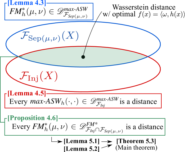
Figure 1: Outline of Sec. 4. Proposition 4.6 is a major step toward our main theorem.

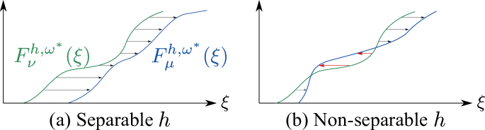
Figure 2: Illustration of Definition 4.2. (a) A separable function $h$ for $\mu$ and $\nu$ satisfies $F_{\mu}^{h,\omega^{*}}(\xi)\geq F_{\nu}^{h,\omega^{*}}(\xi)$ for $\omega^{*}=d_{h}(\mu,\nu)$. (b) For non-separable $h$, $\mathrm{sign}(F_{\mu}^{h,\omega^{*}}(\xi)-F_{\nu}^{h,\omega^{*}}(\xi))$ depends on $\xi$, which necessiates of evaluation of the sign to calculate $\textit{max-ASW}(\mu,\nu;h)$ by Eq. (6) (see Remark 4.4).

4 Conditions for Metrizability: Analysis by Max-ASW

In this section, we provide an answer to Question 3.4.

4.1 Strategy for Answering Question 3.4

We consider the conditions of ${\mathcal{F}}(X)$ for Question 3.4 in the context of sliced optimal transport. To this end, we define a variant of sliced optimal transport, called maximum augmented sliced Wasserstein divergence (max-ASW) in Definition 4.1. In Sec. 4.2, we first introduce a condition, called separable condition, where divergences included in the FM family are also included in the max-ASW family. In Sec. 4.3, we further introduce a condition, called injective condition, where the max-ASW is a distance. Finally, imposing these conditions on ${\mathcal{F}}(X)$ brings us the desired conditions (see Fig. 2 for the discussion flow).

Definition 4.1 (Maximum Augmented Sliced Wasserstein Divergence (max-ASW)).

Given a functional space ${\mathcal{F}}(X)\subseteq L^{\infty}(X,{\mathbb{R}}^{D})$, we define a family of max-ASWs as

$$\mathscr{D}^{\text{max-ASW}}_{\mathcal{F}}:=\left\{(\mu,\nu)\mapsto\!\!\!\!\max_{\omega\in{\mathbb{S}}^{D-1}}\!\!W_{1}\left({\mathcal{S}}^{h}I_{\mu}(\cdot,\omega),{\mathcal{S}}^{h}I_{\nu}(\cdot,\omega)\right)|h\in{\mathcal{F}}(X)\right\}.$$ (13)

Further, we denote an instance of the family as $\textit{max-ASW}_{h}(\mu,\nu)\in\mathscr{D}^{\text{max-ASW}}_{{\mathcal{F}}}$, where $h\in{\mathcal{F}}(X)$.

Note that although the formulation in the definition includes the SRT, similarly to the ASW in Eq. (8), they differ in terms of the method of direction sampling ($\omega$).

4.2 Seperability for Equivalence of FM^∗ and Max-ASW

We introduce a property for the function $h$, called separability (refer to Remark 4.4 for intuitive explanation).

Definition 4.2 (Separable).

Given $\mu,\nu\in{\mathcal{P}}(X)$, let $\omega$ be on $\mathbb{S}^{D-1}$, and let $F_{\mu}^{h,\omega}(\cdot)$ be the cumulative distribution function of ${\mathcal{S}}^{h}I_{\mu}(\cdot,\omega)$. If $\omega^{*}=d_{h}(\mu,\nu)$ satisfies $F_{\mu}^{h,\omega^{*}}(\xi)\leq F_{\nu}^{h,\omega^{*}}(\xi)$ for any $\xi\in{\mathbb{R}}$, $h\in L^{\infty}(X,{\mathbb{R}}^{D})$ is separable for those probability measures. We denote the class of all these separable functions for them as ${\mathcal{F}}_{\text{Sep}(\mu,\nu)}(X)$.

Under this definition, separable functions connect the FM^∗ and the max-ASW as follows.

Lemma 4.3.

Given $\mu,\nu\in{\mathcal{P}}(X)$, every $h\in{\mathcal{F}}_{\text{Sep}(\mu,\nu)}(X)$ satisfies $\textit{FM}_{h}^{*}(\mu,\nu)\in\mathscr{D}^{\text{max-ASW}}_{{\mathcal{F}}_{\text{Sep}(\mu,\nu)}}$.

Remark 4.4.

For a general function $h\in L^{\infty}(X,{\mathbb{R}}^{D})$, $\textit{FM}_{h}^{*}(\cdot,\cdot)$ is not necessarily included in the max-ASW family, i.e., ${\mathcal{D}}(\cdot,\cdot)\in\mathscr{D}^{\text{max-ASW}}_{{\mathcal{F}}}(\cdot,\cdot)\not\Leftrightarrow{\mathcal{D}}(\cdot,\cdot)\in\mathscr{D}^{\text{FM*}}_{{\mathcal{F}}}$ for general ${\mathcal{F}}(X)\subseteq L^{\infty}(X,{\mathbb{R}}^{D})$. Fig. 2 intuitively illustrates why separability is crucial. Given $h$, calculation of the max-ASW via Eq.  (6) generally involves evaluation of the sign of the difference between the quantile functions. Intuitively, the equivalence between the FM and max-ASW distances holds if the sign is always positive regardless of $\rho\in[0,1]$; otherwise, the sign’s dependence on $\rho$ breaks the equivalence.

4.3 Injectivity for Max-ASW To Be A Distance

Imposing injectivity on $h$ guarantees that the induced max-ASW is indeed a distance.

Lemma 4.5.

Every $\textit{max-ASW}_{h}(\cdot,\cdot)\in\mathscr{D}^{\text{max-ASW}}_{{\mathcal{F}}_{\text{Inj}}}$ is a distance, where ${\mathcal{F}}_{\text{Inj}}$ indicates a class of all the injective functions in $L^{\infty}(X,{\mathbb{R}}^{D})$.

According to Lemmas 4.3 and 4.5, $\textit{FM}_{h}(\mu,\nu)$ with a separable and injective $h$ is indeed a distance since it is included in the family of max-ASW distances. With Proposition 4.6, we have now one of the answers to Question 3.4, which hints us our main theorem.

Proposition 4.6.

Given $\mu,\nu\in{\mathcal{P}}(X)$, every $\textit{FM}_{h}^{*}(\mu,\nu)\in\mathscr{D}^{\text{FM*}}_{{\mathcal{F}}_{\text{Inj}}\cap{\mathcal{F}}_{\text{Sep}(\mu,\nu)}}$ is indeed a distance.

5 GAN Training Indeed Minimizes Distance?

We present Theorem 5.3, which is our main theoretical result and gives sufficient conditions for the discriminator to be ${\mathcal{J}}$-metrizable. Then, we explain certain implications of the theorem.

5.1 Metrizable Discriminator in GAN

We directly apply the discussion in the previous section to ${\mathcal{J}}_{\text{Wass}}$, and by extending the result for Wasserstein GAN to a general GAN, we derive the main result.

First, a simple combination of Propositions 3.5 and 4.6 yields the following lemma.

Lemma 5.1 (${\mathcal{J}}_{\text{Wass}}$-metrizable).

Given $h\in{\mathcal{F}}_{\text{Inj}}\cap{\mathcal{F}}_{\text{Sep}(\mu_{0},\mu_{\theta})}$ with ${\mathcal{F}}_{\text{Inj}},{\mathcal{F}}_{\text{Sep}(\mu_{0},\mu_{\theta})}\subseteq L^{\infty}(X,{\mathbb{R}}^{D})$, let $\omega^{*}\in{\mathbb{S}}^{D-1}$ be $\hat{d}_{h}(\mu_{0},\mu_{\theta})$. Then $f(x)=\langle{\omega,h(x)}\rangle$ is $({\mathcal{J}}_{\text{Wass}},\textit{FM}_{h}^{*})$-metrizable.

Lemma 5.1 provides the conditions for the discriminator to be ${\mathcal{J}}_{\text{Wass}}$-metrizable.

Next, we generalize this result to more generic minimization problems. The scope is minimization problems of general GANs that are formalized in the form ${\mathcal{J}}(\theta;f)=\mathbb{E}_{x\sim\mu_{\theta}}[R_{\mathcal{J}}\circ f(x)]$ with $R_{\mathcal{J}}:{\mathbb{R}}\to{\mathbb{R}}$. We use the gradient of such minimization problems w.r.t. $\theta$:

$$\nabla_{\theta}{\mathcal{J}}(\theta;f)=-\mathbb{E}_{z\sim\sigma}\left[r_{\mathcal{J}}\circ f(g_{\theta}(z))\nabla_{\theta}f(g_{\theta}(z))\right],$$ (14)

where $r_{\mathcal{J}}(\cdot)$ is the derivative of $R_{\mathcal{J}}(\cdot)$ as listed in Table 2. By ignoring a scaling factor, Eq. (14) can be regarded as a gradient of $d_{f}(\tilde{\mu}_{0}^{r_{\mathcal{J}}\circ f},\tilde{\mu}_{\theta}^{r_{\mathcal{J}}\circ f})$, where $\tilde{\mu}^{r\circ f}$ is defined via $I_{\tilde{\mu}^{r\circ f}}(x)\propto r\circ f(x)I_{\mu}(x)$. To examine whether updating the generator with the gradient in Eq. (14) can minimize a certain distance between $\mu_{0}$ and $\mu_{\theta}$, we introduce the following lemma.

Lemma 5.2.

For any $\rho:X\to{\mathbb{R}}_{+}$ and a distance for probability measures ${\mathcal{D}}(\cdot,\cdot)$, ${\mathcal{D}}(\tilde{\mu}^{\rho},\tilde{\nu}^{\rho})$ indicates a distance between $\mu$ and $\nu$.

By leveraging Lemma 5.2 and applying Propositions 3.5 and 4.6 to $\tilde{\mu}_{0}^{r_{\mathcal{J}}\circ f}$ and $\tilde{\mu}_{\theta}^{r_{\mathcal{J}}\circ f}$, we finally derive the ${\mathcal{J}}$-metrizable conditions for $\mu_{0}$ and $\mu_{\theta}$, which is our main result.

Theorem 5.3 (${\mathcal{J}}$-Metrizability).

Given a functional ${\mathcal{J}}(\theta;f):=\mathbb{E}_{x\sim\mu_{\theta}}[R\circ f(x)]$ with $R^{\prime}(\cdot):{\mathbb{R}}\to{\mathbb{R}}_{+}$, let $h\in L^{\infty}(X,{\mathbb{R}}^{D})$ and $\omega\in{\mathbb{S}}^{D-1}$ satisfy the following conditions:

• (Direction optimality) $\omega=\mathrm{arg~{}max}_{\tilde{\omega}\in{\mathbb{S}}^{D-1}}d_{\langle{\tilde{\omega}},h\rangle}(\tilde{\mu}_{0}^{R^{\prime}\circ f},\tilde{\mu}_{\theta}^{R^{\prime}\circ f})$,

• (Separability) $h$ is separable for $\tilde{\mu}_{0}^{R^{\prime}\circ f}$ and $\tilde{\mu}_{\theta}^{R^{\prime}\circ f}$,

• (Injectivity) $h$ is an injective function.

Then $f(x)=\langle{\omega,h(x)}\rangle$ is ${\mathcal{J}}$-metrizable for $\mu_{\theta}$ and $\mu_{0}$.

We refer to the conditions in Theorem 5.3 as metrizable conditions. According to the theorem, the discriminator $f=\langle\omega,h\rangle$ can serve as a distance between the generator and target distributions even if it is not the optimal solution to the original maximization problem ${\mathcal{V}}$.

5.2 Implications of Theorem 5.3

We are interested in the question of whether discriminators in existing GANs can satisfy the metrizable conditions. We summarize our observations in Table 1.

First, as explained in the next section, most existing GANs besides Wasserstein GAN do not satisfy direction optimality with the maximizer $\omega$ of ${\mathcal{V}}$. This fact inspires us to develop novel maximization objectives (see Sec. 6). Second, it is generally hard to make the function $h$ rigorously satisfy separability, or verify that it is really satisfied. In Appx. E, a simple experiment demonstrates that Wasserstein GAN tends to fail to learn separable functions. Third, the property of injectivity largely depends on the discriminator design. There are various ways to impose injectivity on the discriminator. One way is to implement the discriminator with an invertible neural network. Although this topic has been actively studied (Behrmann et al., 2019; Karami et al., 2019; Song et al., 2019), such networks have higher computational costs for training (Chen et al., 2022). Another way is to add regularization terms to the maximization problem. For example, a gradient penalty (GP) (Gulrajani et al., 2017) can promote injectivity by explicitly regularizing the discriminator’s gradient. In contrast, simple removal of operators that can destroy injectivity, such as ReLU activation, can implicitly overcome this issue. We empirically verify this discussion in Sec. 7.1 and Appx. E.

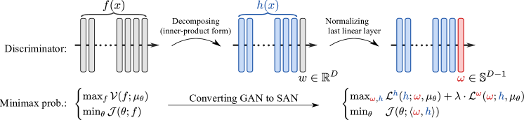
Figure 3: Converting GAN to SAN involves only simple modifications to discriminators.

6 Slicing Adversarial Network

This section describes our proposed model, the Slicing Adversarial Network (SAN) to achieve the direction optimality in Theorem 5.3. We develop the SAN by modifying the maximization problem on ${\mathcal{V}}$ to guarantee that the optimal solution $\omega$ achieves direction optimality. The proposed modification scheme is applicable to most existing GAN objectives and does not necessitate additional exhaustive hyperparameter tuning and computational complexity.

As mentioned in Sec. 5.1, given a function $h$, maximization problems in most GANs (besides Wasserstein GAN) cannot achieve direction optimality with the maximum solution of ${\mathcal{V}}$, as reported in Table 1. We use hinge GAN as an example to illustrate this claim. The objective function to be maximized in hinge GAN is formulated as

$${\color[rgb]{0,0,0}{{{\mathcal{V}}_{\text{Hinge}}(\langle\omega,h\rangle;\mu_{\theta}):=\mathbb{E}_{x\sim\mu_{0}}[\min(0,-1+\langle\omega,h(x)\rangle)]+\mathbb{E}_{x\sim\mu_{\theta}}[\min(0,-1-\langle\omega,h(x)\rangle)].}}}$$ (15)

Given $h$, the maximizer $\omega$ becomes $\hat{d}_{h}(\mu_{0}^{\text{tr}},\mu_{\theta}^{\text{tr}})$, where $\mu_{0}^{\text{tr}}$ and $\mu_{\theta}^{\text{tr}}$ denote truncated distributions whose supports are restricted by conditioning $x$ on $\langle\omega,h(x)\rangle<1$ and $\langle\omega,h(x)\rangle>-1$, respectively. Because $(\mu_{0}^{\text{tr}},\mu_{\theta}^{\text{tr}})$ is generally different from $(\tilde{\mu}_{0}^{r_{\mathcal{J}}},\tilde{\mu}_{\theta}^{r_{\mathcal{J}}})=(\mu_{0},\mu_{\theta})$, the maximum solution does not satisfy direction optimality for $\tilde{\mu}_{0}^{r_{\mathcal{J}}}$ and $\tilde{\mu}_{\theta}^{r_{\mathcal{J}}}$.

In line with the above discussion, we propose the following novel maximization problem:

$${\color[rgb]{0,0,0}{{\max_{\omega\in\mathbb{S}^{d-1},h\in{\mathcal{F}}(X)}{\mathcal{V}}^{\text{SAN}}(\omega,h;\mu_{\theta}):=\underbrace{{\mathcal{V}}(\langle\omega^{-},h\rangle;\mu_{\theta})}_{{\mathcal{L}}^{h}(h;\omega,\mu_{\theta})}+\lambda\cdot\underbrace{d_{\langle\omega,h^{-}\rangle}(\tilde{\mu}_{0}^{r_{\mathcal{J}}\circ f},\tilde{\mu}_{\theta}^{r_{\mathcal{J}}\circ f})}_{{\mathcal{L}}^{\omega}(\omega;h,\mu_{\theta})},}}}$$ (16)

where $(\cdot)^{-}$ indicates a stop-gradient operator and has zero partial derivatives. We simply set $\lambda\in{\mathbb{R}}$ to 1 in our experiments. The proposed modification scheme in Eq. (16) enables us to select any maximization objective for $h$ with ${\mathcal{L}}^{h}$, while ${\mathcal{L}}^{\omega}$ enforces direction optimality on $\omega$. Hence, we can convert most GAN maximization problem to SAN problem using Eq. (16). One can easily extend SAN to class conditional generation by introducing directions for respective classes (see Appx. B).

Table 2: Minimization problem and weighting function for direction optimization.

	Minimization problem ${\mathcal{J}}$	Weighting $r_{\mathcal{J}}\circ f(x)$
Wasserstein GAN / Hinge GAN	$-\mathbb{E}_{x\sim\mu_{\theta}}\left[f(x)\right]$	1
Saturating GAN	$-\mathbb{E}_{x\sim\mu_{\theta}}\left[\log\varsigma(f(x))\right]$	$1-\varsigma(f(x))$
Non-saturating GAN	$\mathbb{E}_{x\sim\mu_{\theta}}\left[\log\varsigma(1-f(x))\right]$	$\varsigma(f(x))$

One of SAN’s strength is that the model can be trained with two small modifications to existing GAN implementations (see Fig. 3 and Appx. A). The first is to implement the discriminator’s last linear layer to be on a hypersphere as $f_{\varphi}(x)=w_{\varphi_{L}}^{\top}h_{\varphi_{<L}}(x)$ with $w_{\varphi_{L}}\in{\mathbb{S}}^{D-1}$, where $\varphi_{l}$ is the parameter for the $l$th layer. The second is to use the maximization problem defined in Eq. (16).

Comparison with other generative models.   First, SAN can be compared with GAN. In GAN, other than Wasserstein GAN, the optimal discriminator is known to involve a dilemma: it induces a certain dissimilarity but leads to exploding and vanishing gradients (Arjovsky et al., 2017; Lin et al., 2021). In contrast, in SAN, the metrizable conditions ensure that the optimal discriminator is not necessary to obtain a metrizable discriminator. Next, similarly to variants of the maximum SW (Deshpande et al., 2019; Kolouri et al., 2019), the SAN’s discriminator is interpreted as extracting features $h(x)$ and slicing them in the most distinctive direction $\omega$. In the conventional methods, one-dimensional Wasserstein distances are approximated by sample sorting (see Remark 4.4). It has been reported that the generation performances get better when the batch size increases (Nguyen et al., 2021; Chen et al., 2022). However, larger batch size leads to slower training speed, and the size is capped by memory constraints. In contrast, SANs remove the necessity of the approximation.

7 Experiments

We perform experiments with synthetic and image datasets (1) to verify our perspective on GANs as presented in Sec. 5 in terms of direction optimality, separability, and injectivity, and (2) to show the effectiveness of SAN against GAN. For fair comparisons, we essentially use the same architectures in SAN and GAN. However, we modify the last linear layer of SAN’s discriminators (see Sec. 6).

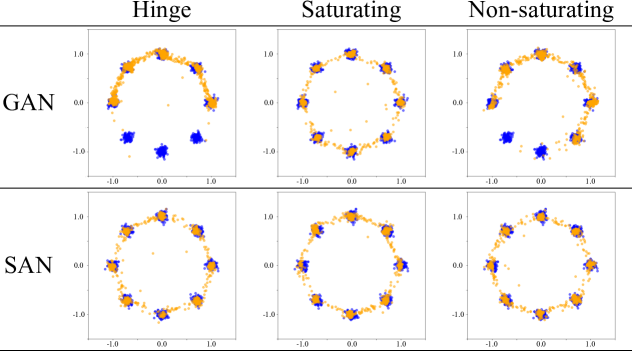
Figure 4: Comparison of the learned distributions (at 10,000 iterations) between GAN and SAN with various objectives. In all cases, SANs cover all modes whereas mode collapse occurs in some GAN cases.

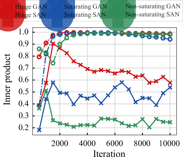
Figure 5: Inner product of trained $\omega$ and numerically estimated optimal direction for $\tilde{\mu}_{0}^{r_{\mathcal{J}}}$ and $\tilde{\mu}_{\theta}^{r_{\mathcal{J}}}$ during training. The trained $\omega$ were closer to the optimal direction with SAN than with GAN.

Table 3: FID scores ($\downarrow$) on DCGAN.

Dataset	Hinge loss		Saturating loss		Non-saturating loss
GAN	SAN	GAN	SAN	GAN	SAN
CIFAR10	24.07$\pm$0.56	20.23$\pm$0.86	25.63$\pm$0.98	20.62$\pm$0.94	24.90$\pm$0.21	20.51$\pm$0.36
CelebA	32.51$\pm$2.53	27.79$\pm$1.60	37.33$\pm$1.02	28.16$\pm$1.60	28.22$\pm$2.16	27.78$\pm$4.59

Table 4: FID and IS results on CIFAR10 with the experimental setup of BigGAN (Brock et al., 2019). Scores marked with $*$ are results from our implementation, which is based on BigGAN author’s PyTorch implementation. For reference, scores reported in their paper are put with $\dagger$.

Metric	Unconditional		Conditional
Hinge GAN∗	Hinge SAN∗	Hinge GAN†	Hinge GAN∗	Hinge SAN∗
FID ($\downarrow$)	17.16$\pm$1.34	14.45$\pm$0.58	14.73	8.25$\pm$0.82	6.20$\pm$0.27
IS ($\uparrow$)	8.42$\pm$0.11	8.81$\pm$0.04	9.22	9.05$\pm$0.05	9.16$\pm$0.08

Table 5: Numerical results for StyleGAN-XL (Sauer et al., 2022) and StyleSAN-XL on ImageNet (256$\times$256). Scores marked with $\dagger$ are reported in their paper.

Method	FID ($\downarrow$)	IS ($\uparrow$)
StyleGAN-XL†	2.30	265.12
StyleSAN-XL	2.14	274.20

7.1 Mixture of Gaussians

To empirically investigate optimal direction, we conduct experiments on a mixture of Gaussian (MoG). Please refer to Appx. E for empirical verification of implications of Theorem 5.3 regarding separability and injectivity. We use a two-dimensional sample space $X={\mathbb{R}}^{2}$. The target MoG on $X$ comprises eight isotropic Gaussians with variances $0.05^{2}$ and means distributed evenly on a circle of radius $1.0$. We use a 10-dimensional latent space $Z$ to model a generator measure.

We compare SAN and GAN with various objectives. As shown in Fig. 5, the generator measures trained with SAN cover all modes whereas mode collapse (Srivastava et al., 2017) occurs with hinge GAN and non-saturating GAN. In addition, Fig. 5 shows a plot of the inner product of the learned direction $\omega$ (or the normalized weight in GAN’s last linear layer) and the estimated optimal direction for $\tilde{\mu}_{0}^{r_{\mathcal{J}}}$ and $\tilde{\mu}_{\theta}^{r_{\mathcal{J}}}$. Recall that there is no guarantee that a non-optimal direction $\omega$ induces a distance.

7.2 Image Generation

We apply SANs to several image generation tasks to show they scale beyond toy experiments.

DCGAN.   We train SANs and GANs with various objective functions on CIFAR10 (Krizhevsky et al., 2009) and CelebA (128$\times$128) (Liu et al., 2015). We adopt the DCGAN architectures (Radford et al., 2016), and for the discriminator, we apply spectral normalization (Miyato et al., 2018). As reported in Table 5, SANs outperform GANs in terms of the FID score in all cases.

BigGAN.   Next, we apply SAN to BigGAN (Brock et al., 2019) on CIFAR10. In this experiment, we calculate the Inception Score (IS) (Salimans et al., 2016), as well as the FID, to evaluate the sample quality by following the experiment in the original paper. As in Table 5, the adoption of SAN consistently improves the generation performance in terms of both metrics.

StyleGAN-XL.   Lastly, we apply our SAN training framework to StyleGAN-XL (Sauer et al., 2022), which is a state-of-the-art GAN-based generative model. We name the StyleGAN-XL model combined with our SAN training framework StyleSAN-XL. We train StyleSAN-XL on ImageNet (256$\times$256) (Russakovsky et al., 2015) and report the FID and IS as with BigGAN. As shown in Table 5, SAN boosts even the generation performance of the state-of-the-art GAN-based generative model. Our code for StyleSAN-XL is available at https://github.com/sony/san.

8 Conclusion

We first proposed a novel perspective on GANs to derive sufficient conditions for the discriminator to serve as a distance between the data and generator probability measures. To this end, we introduced the FM^∗ and max-ASW families. By using a class of metrics that are included in both families, we derived the metrizable conditions for Wasserstein GAN. We then extended the result to a general GAN. The derived conditions consist of direction optimality, separability, and injectivity.

By leveraging the theoretical results, we proposed SAN, in which a generator and discriminator are trained with a modified GAN training scheme. This model can impose direction optimality on the discriminator despite the ease of modifications and the generality. SANs experimentally outperformed GANs on synthetic and image datasets in terms of the sample quality and mode coverage.

Appendix A Converting GANs to SANs

One can convert GANs to SANs only by adding two modifications to existing GAN implementations as in Fig. 3. First, we propose to modify the last linear layer of the discriminator as in the following PyTorch-like code snippet. In the code snippet, feature_network represents any feature extractor $h(\cdot)$ built with nonlinear layers. On top of it, we propose to use the novel maximization objective functions $\mathcal{L}^{h}$ and $\mathcal{L}^{\omega}$. The discriminator’s outputs, out_fun and out_dir, are used for $\mathcal{L}^{h}$ and $\mathcal{L}^{\omega}$, respectively.

⬇

1import torch.nn as nn

2

3class GANDiscriminator(nn.Module):

4 def __init__(self,

5 dim # dimension of output of "h(x)"

6 ):

7 super(GANDiscriminator, self).__init__()

8

9 self.main = feature_network(dim) # nonlinear function "h(x)"

10 self.fc = nn.Linear(dim, 1) # last linear layer "w"

11

12 def forward(self,

13 x # batch of real/fake samples

14 ):

15 feature = self.main(x)

16 out = self.fc(feature)

17

18 return out

Listing 1: GAN’s discriminator

⬇

1import torch

2import torch.nn as nn

3import torch.nn.functional as F

4

5class SANDiscriminator(nn.Module):

6 def __init__(self,

7 dim # dimension of output of "h(x)"

8 ):

9 super(SANDiscriminator, self).__init__()

10

11 self.main = feature_network(dim) # nonlinear function "h(x)"

12 vec_init = torch.randn(dim, ) # initialization for direction

13 self.vec = nn.Parameter(vec_init) # unnormalized direction

14

15 def forward(self,

16 x # batch of real/fake samples

17 ):

18 feature = self.main(x)

19 direction = F.normalize(self.vec, dim=0) # direction "omega"

20 out_fun = feature @ direction.detach()

21 out_dir = feature.detach() @ direction

22

23 return out_fun, out_dir

Listing 2: SAN’s discriminator

As an example, converting the maximization objective of Hinge GAN to SAN leads to

$$\mathcal{V}_{\text{Hinge}}^{\text{SAN}}(\omega,h;\mu_{\theta})=\underbrace{\mathcal{V}_{\text{Hinge}}(\langle\omega^{-},h\rangle,\mu_{\theta})}_{\mathcal{L}^{h}}+\lambda\cdot\underbrace{\mathcal{V}_{\text{Wass}}(\langle\omega,h^{-}\rangle,\mu_{\theta})}_{\mathcal{L}^{\omega}}.$$ (17)

For general GANs, the approximations of $\tilde{\mu}_{0}^{r_{\mathcal{J}}\circ f}$ and $\tilde{\mu}_{\theta}^{r_{\mathcal{J}}\circ f}$ are needed. The objective term $\mathcal{L}^{\omega}$ can be formulated as

$${\color[rgb]{0,0,0}{{\mathcal{L}^{\omega}(\omega;h,\mu_{\theta})=\frac{1}{Z_{0}}\mathbb{E}_{x\sim\mu_{0}}[r_{\mathcal{J}}\circ f^{-}(x)\langle{\omega,h(x)}\rangle]-\frac{1}{Z_{\theta}}\mathbb{E}_{x\sim\mu_{\theta}}[r_{\mathcal{J}}\circ f^{-}(x)\langle{\omega,h(x)}\rangle]}}},$$ (18)

where $Z_{0}=\mathbb{E}_{x\sim\mu_{0}}[r_{\mathcal{J}}\circ f^{-}(x)]$ and $Z_{\theta}=\mathbb{E}_{x\sim\mu_{\theta}}[r_{\mathcal{J}}\circ f^{-}(x)]$. The normalizing terms $Z_{0}$ and $Z_{\theta}$ can be approximated per batch. However, we found it beneficial to use the following auxiliary objective function instead:

$${\color[rgb]{0,0,0}{{\mathcal{L}_{\text{simple}}^{\omega}(\omega;h,\mu_{\theta})=\mathbb{E}_{x\sim\mu_{0}}[R_{\mathcal{J}}(\langle{\omega,h}\rangle)]-\mathbb{E}_{x\sim\mu_{\theta}}[R_{\mathcal{J}}(\langle{\omega,h}\rangle)]}}},$$ (19)

which ignores the normalization terms $Z_{0}$ and $Z_{\theta}$ in Eq. (19).

Appendix B Class Conditional SAN

SAN can easily be extended to conditional generation. Let $C$ be the number of classes. For a conditional case, we adopt the usual generator parameterization, $g_{\theta}:Z\times\{c\}_{c=1}^{C}\to X$, which gives a conditional generator distribution $\mu_{\theta}^{c}:=g_{\theta}(\cdot,c){{}_{\sharp}}\sigma$. For the discriminator, we prepare trainable directions for the respective classes as $\Omega:=\{\omega_{c}\}_{c=1}^{C}$. Under this setup, we define the minimax problem of conditional SAN as follows:

$$\max_{\Omega,h}\mathbb{E}_{c\sim P(c)}\left[{\mathcal{V}}_{\mu_{0}^{c}}^{\text{SAN}}(\omega_{c},h;\mu_{\theta}^{c})\right]\quad\text{and}\quad\min_{\theta}\mathbb{E}_{c\sim P(c)}\left[{\mathcal{J}}(\theta;\langle{\omega_{c},h}\rangle)\right],$$ (20)

where $P(c)$ is a pre-fix probability mass function for $c$, and $\mu_{0}^{c}$ is the target probability measure conditioned on $c$.

Even for conditional generation, GAN can easily be converted into SAN, because many previous works implemented a conditional discriminator with a class-conditional last layer as $w_{\phi_{L},c}^{\top}h_{\phi_{<L}}(x)$ (Miyato & Koyama, 2018; Miyato et al., 2018; Brock et al., 2019; Zhang et al., 2019).

Appendix C Proofs

Proposition 3.2. For ${\mathcal{F}}(X)\in L^{\infty}(X,{\mathbb{R}})$, $\textit{IPM}_{{\mathcal{F}}}(\cdot,\cdot):=\max_{f\in{\mathcal{F}}}d_{f}(\cdot,\cdot)\in\mathscr{D}^{\text{FM}}_{1}$.

Proof.

The claim is direct consequence of the definitions of the IPM and the FM. ∎

We introduce a lemma, which will come in handy in the proofs of Proposition 3.5 and Lemma 4.3.

Lemma C.1.

Given a function $h\in L^{\infty}(X,{\mathbb{R}}^{D})$ and probability measures $\mu,\nu\in{\mathcal{P}}(X)$, we have

$$\|d_{h}(\mu,\nu)\|_{2}=\max_{\omega\in{\mathbb{S}}^{D-1}}d_{\langle\omega,h\rangle}(\mu,\nu).$$ (21)

Proof.

From the Cauchy–Schwarz inequality, we have the following lower bound using $\omega\in{\mathbb{S}}^{D-1}$:

$$\|d_{h}(\mu,\nu)\|_{2} =\|\mathbb{E}_{x\sim\mu}[h(x)]-\mathbb{E}_{x\sim\nu}[h(x)]\|_{2}$$

$$\geq\langle\omega,\mathbb{E}_{x\sim\mu}[h(x)]-\mathbb{E}_{x\sim\nu}[h(x)]\rangle,$$ (22)

where the equality holds if and only if $\omega=\hat{d}(\mu,\nu)$. Remind that $\hat{(\cdot)}$ denotes a normalization operator. Then, calculating the norm $\|d_{h}(\mu,\nu)\|_{2}$ is formulated as the following maximization problem:

$$\|d_{h}(\mu,\nu)\|_{2} =\max_{\omega\in{\mathbb{S}}^{D-1}}\mathbb{E}_{x\sim\mu}[\langle\omega,h(x)\rangle]-\mathbb{E}_{x\sim\nu}[\langle\omega,h(x)\rangle]$$ (23)

$$=\max_{\omega\in{\mathbb{S}}^{D-1}}d_{\langle\omega,h\rangle}(\mu,\nu).$$ (24)

Note that we can interchange the inner product and the expectation operator by the independency of $\omega$ w.r.t. $x$. ∎

Proposition 3.5. Let $\omega$ be on ${\mathbb{S}}^{D-1}$. For any $h\in L^{\infty}(X,{\mathbb{R}}^{D})$, minimization of $\textit{FM}_{h}^{*}(\mu_{\theta},\mu_{0})$ is equivalent to optimization of $\min_{\theta\in{\mathbb{R}}^{D_{\theta}}}\max_{\omega\in{\mathbb{S}}^{D-1}}{\mathcal{J}}_{\text{Wass}}(\theta;\langle{\omega,h}\rangle)$. Thus,

$$\nabla_{\theta}\textit{FM}_{h}^{*}(\mu_{\theta},\mu_{0})=\nabla_{\theta}{\mathcal{J}}_{\text{Wass}}(\theta;\langle{\omega^{*},h}\rangle),$$ (25)

where $\omega^{*}$ is the optimal solution (direction) given as follows:

$$\omega^{*}=\mathop{\rm arg~{}max}\limits_{\omega\in{\mathbb{S}}^{D-1}}~{}d_{\langle{\omega,h}\rangle}(\mu_{0},\mu_{\theta}).$$ (26)

Proof.

From Lemma C.1, we have

$$\|d_{h}(\mu_{0},\mu_{\theta})\|_{2} =\max_{\omega\in{\mathbb{S}}^{D-1}}d_{\langle\omega,h\rangle}(\mu_{0},\mu_{\theta})$$ (27)

$$=\max_{\omega\in{\mathbb{S}}^{D-1}}\mathbb{E}_{x\sim\mu_{0}}[\langle\omega,h(x)\rangle]-\mathbb{E}_{x\sim\mu_{\theta}}[\langle\omega,h(x)\rangle]$$ (28)

By a simple envelope theorem (Milgrom & Segal, 2002), we have

$$\nabla_{\theta}\|d_{h}(\mu_{0},\mu_{\theta})\|_{2} =\nabla_{\theta}\left(\mathbb{E}_{x\sim\mu_{0}}[\langle\omega^{*},h(x)\rangle]-\mathbb{E}_{x\sim\mu_{\theta}}[\langle\omega^{*},h(x)\rangle]\right)$$ (29)

where $\omega^{*}=\max_{\omega\in{\mathbb{S}}^{D-1}}d_{\langle\omega,h\rangle}(\mu_{0},\mu_{\theta})$. Since the first term in the right-hand side in Eq. (29) does not depend on $\theta$, taking gradient of $\|d_{h}(\mu_{0},\mu_{\theta})\|_{2}$ w.r.t. $\theta$ becomes

$$\nabla_{\theta}\|d_{h}(\mu_{0},\mu_{\theta})\|_{2} =-\nabla_{\theta}\mathbb{E}_{x\sim\mu_{\theta}}[\langle\omega^{*},h(x)\rangle].$$ (30)

Substituting the definition of ${\mathcal{J}}_{\text{Wass}}$ and $\textit{FM}^{*}_{h}(\cdot,\cdot)$ into Eq. (30) leads to the equality in the statement of Proposition 3.5. ∎

Lemma 4.3. Given $\mu,\nu\in{\mathcal{P}}(X)$, every $h\in{\mathcal{F}}_{\text{Sep}(\mu,\nu)}(X)$ satisfies $\textit{FM}_{h}^{*}(\mu,\nu)\in\mathscr{D}^{\text{max-ASW}}_{{\mathcal{F}}_{\text{Sep}(\mu,\nu)}}$.

Proof.

From Lemma C.1, we have

$$\|d_{h}(\mu,\nu)\|_{2} =\max_{\omega\in{\mathbb{R}}^{D-1}}\mathbb{E}_{x\sim\mu}[\langle\omega,h(x)\rangle]-\mathbb{E}_{x\sim\nu}[\langle\omega,h(x)\rangle]$$ (31)

$$=\mathbb{E}_{x\sim\mu}[\langle\omega^{*},h(x)\rangle]-\mathbb{E}_{x\sim\nu}[\langle\omega^{*},h(x)\rangle],$$ (32)

where, the maximizer is $\omega^{*}=\hat{d}_{h}(\mu,\nu)$.

The expected values are reformulated by the SRT as

$$\mathbb{E}_{x\sim\mu}[\langle\omega,h(x)\rangle] =\int_{X}\left(\int_{\mathbb{R}}\xi\delta(\xi-\langle\omega,h(x)\rangle)d\xi\right)I_{\mu}(x)dx$$ (33)

$$=\int_{\mathbb{R}}\xi\left(\int_{X}I_{\mu}(x)\delta(\xi-\langle\omega,h(x)\rangle)dx\right)d\xi$$ (34)

$$=\mathbb{E}_{\xi\sim{\mathcal{S}}^{h}I_{\mu}(\xi,\omega)}[\xi].$$ (35)

The interchange of the integral follows from the Fubini theorem. Here, the applicability of the theorem is justified by the absolute integrability of the integrant function. That is, $\int_{X}\|h(x)\|_{2}d\mu(x)\leq\|h\|_{L^{\infty}(X,{\mathbb{R}}^{D})}\mu(X)=\|h\|_{L^{\infty}(X,{\mathbb{R}}^{D})}<\infty$.

Further, the right-hand side of Eq. (35) follows the representation of an expectation by an integral of quantiles:

$$\mathbb{E}_{\xi\sim{\mathcal{S}}^{h}I_{\mu}(\xi,\omega)}[\xi]=\int_{0}^{1}Q_{\mu}^{h,\omega}(\rho)d\rho$$ (36)

By substituting Eqs. (35) and (36) into Eq. (32), we have

$$\|d_{h}(\mu,\nu)\|_{2}=\int_{0}^{1}\left(Q_{\mu}^{h,\omega^{*}}(\rho)-Q_{\nu}^{h,\omega^{*}}(\rho)\right)d\rho.$$ (37)

The right-hand side of Eq. (37) is bounded above:

$$\|d_{h}(\mu,\nu)\|_{2}\leq\int_{0}^{1}\left|Q_{\mu}^{h,\omega^{*}}(\rho)-Q_{\nu}^{h,\omega^{*}}(\rho)\right|d\rho.$$ (38)

The equality holds if and only if $Q_{\mu}^{h,\omega^{*}}(\rho)-Q_{\nu}^{h,\omega^{*}}(\rho)\geq 0$ for all $\rho$ or $Q_{\mu}^{h,\omega^{*}}(\rho)-Q_{\nu}^{h,\omega^{*}}(\rho)\leq 0$ for all $\rho$. By considering the fact that selecting $-\omega$ changes the sign and Eq. (37) is non-negative, the necessary and sufficient condition for the equality becomes $Q_{\mu}^{h,\omega^{*}}(\rho)-Q_{\nu}^{h,\omega^{*}}(\rho)\geq 0$ for $\rho\in[0,1]$. From the monotonicity of quantile functions, the condition for the equality is written as $F_{\mu}^{h,\omega}(\rho)\leq F_{\nu}^{h,\omega}(\rho)$. ∎

We here borrow a lemma from Chen et al. (2022), which is used in the proof of Lemma 4.5.

Lemma C.2 (Chen et al. (2022), Lemma 1).

Given an injective function $h:X\to{\mathbb{R}}^{D}$ and two probability measures $\mu,\nu\in{\mathcal{P}}(X)$, for all $\xi\in{\mathbb{R}}$ and $\omega\in{\mathbb{S}}^{D-1}$, ${\mathcal{S}}^{h}I_{\mu}(\xi,\omega)={\mathcal{S}}^{h}I_{\nu}(\xi,\omega)$ if and only if $\mu=\nu$.

Lemma 4.5. Every $\textit{max-ASW}_{h}(\cdot,\cdot)\in\mathscr{D}^{\text{max-ASW}}_{{\mathcal{F}}_{\text{Inj}}}$ is a distance, where ${\mathcal{F}}_{\text{Inj}}$ indicates a class of injective functions in $L^{\infty}(X,{\mathbb{R}}^{D})$.

Proof.

One can prove this claim by following similar procedures to the proof of Proposition 1 in Kolouri et al. (2019).

First, the non-negativity and symmetry properties are immediately proven by the fact that Wasserstein distance is indeed a distance satisfying non-negatibity and symmetry.

Next, let $\omega^{*}$ denote

$$\omega^{*}=\mathop{\rm arg~{}max}\limits_{\omega\in{\mathbb{S}}^{D-1}}W_{1}({\mathcal{S}}^{h}I_{\mu_{1}}(\cdot,\omega),{\mathcal{S}}^{h}I_{\mu_{2}}(\cdot,\omega)).$$ (39)

Pick $\nu\in\mathcal{P}(X)$ arbitrarily. The triangle inequality with $\textit{max-ASW}_{h}(\cdot,\cdot)$ is satisfied since

$$\textit{max-ASW}_{h}(\mu_{1},\mu_{2}) =\max_{\omega\in{\mathbb{S}}^{D-1}}W_{1}({\mathcal{S}}^{h}I_{\mu_{1}}(\cdot,\omega),{\mathcal{S}}^{h}I_{\mu_{2}}(\cdot,\omega))$$

$$=W_{1}({\mathcal{S}}^{h}I_{\mu_{1}}(\cdot,\omega^{*}),{\mathcal{S}}^{h}I_{\mu_{2}}(\cdot,\omega^{*}))$$

$$\leq W_{1}({\mathcal{S}}^{h}I_{\mu_{1}}(\cdot,\omega^{*}),{\mathcal{S}}^{h}I_{\nu}(\cdot,\omega^{*}))+W_{1}({\mathcal{S}}^{h}I_{\nu}(\cdot,\omega^{*}),{\mathcal{S}}^{h}I_{\mu_{2}}(\cdot,\omega^{*}))$$ (40)

$$\leq\max_{\omega\in{\mathbb{R}}^{D-1}}W_{1}({\mathcal{S}}^{h}I_{\mu_{1}}(\cdot,\omega),{\mathcal{S}}^{h}I_{\nu}(\cdot,\omega^{*}))$$

$$\qquad+\max_{\omega\in{\mathbb{R}}^{D-1}}W_{1}({\mathcal{S}}^{h}I_{\nu}(\cdot,\omega^{*}),{\mathcal{S}}^{h}I_{\mu_{2}}(\cdot,\omega))$$ (41)

$$=\textit{max-ASW}_{h}(\mu_{1},\nu)+\textit{max-ASW}_{h}(\nu,\mu_{2}).$$ (42)

We show the identity of indiscernibles. For any $\mu$, from $W_{1}(\mu,\mu)=0$, we have $W_{1}({\mathcal{S}}^{h}I_{\mu}(\cdot,\omega),{\mathcal{S}}^{h}I_{\mu}(\cdot,\omega))=0$; therefore, $\textit{max-ASW}_{h}(\mu,\mu)=0$. Conversely, $\textit{max-ASW}_{h}(\mu,\nu)=0$ is equivalent to ${\mathcal{S}}^{h}I_{\mu}(\cdot,\omega)={\mathcal{S}}^{h}I_{\nu}(\cdot,\omega)$ for any $\omega\in{\mathbb{S}}^{D-1}$. This holds if and only if and $\mu=\nu$ from the injectivity assumption on $h$ and Lemma C.2. Therefore $\textit{max-ASW}_{h}(\mu,\nu)=0$ holds if and only if $\mu=\nu$. ∎

Proposition 4.6. Given $\mu,\nu\in{\mathcal{P}}(X)$, every $\textit{FM}_{h}^{*}(\mu,\nu)\in\mathscr{D}^{\text{FM*}}_{{\mathcal{F}}_{\text{Inj}}\cap{\mathcal{F}}_{\text{Sep}(\mu,\nu)}}$ is indeed a distance.

Proof.

The claim is direct consequence of the results of Lemmas 4.3 and 4.5.

From ${\mathcal{F}}_{\text{Inj}}\cap{\mathcal{F}}_{\text{Sep}(\mu,\nu)}\subset{\mathcal{F}}_{\text{Sep}(\mu,\nu)}$ and Lemma 4.3, ${\mathcal{D}}(\mu,\nu)\in\mathscr{D}^{\text{max-ASW}}_{{\mathcal{F}}_{\text{Inj}}\cap{\mathcal{F}}_{\text{Sep}(\mu,\nu)}}$ holds for any ${\mathcal{D}}(\mu,\nu)\in\mathscr{D}^{\text{FM*}}_{{\mathcal{F}}_{\text{Inj}}\cap{\mathcal{F}}_{\text{Sep}(\mu,\nu)}}$. On the other hand, from ${\mathcal{F}}_{\text{Inj}}\cap{\mathcal{F}}_{\text{Sep}(\mu,\nu)}\subset{\mathcal{F}}_{\text{Inj}}$ and Lemma 4.5, ${\mathcal{D}}(\mu,\nu)\in\mathscr{D}^{\text{max-ASW}}_{{\mathcal{F}}_{\text{Inj}}\cap{\mathcal{F}}_{\text{Sep}(\mu,\nu)}}$ is a distance. Thus, the claim is proven. ∎

Lemma 5.1. Given $h\in{\mathcal{F}}_{\text{Inj}}\cap{\mathcal{F}}_{\text{Sep}(\mu_{0},\mu_{\theta})}$ with ${\mathcal{F}}_{\text{Inj}},{\mathcal{F}}_{\text{Sep}(\mu_{0},\mu_{\theta})}\subseteq L^{\infty}(X,{\mathbb{R}}^{D})$, let $\omega^{*}\in{\mathbb{S}}^{D-1}$ be $\hat{d}_{h}(\mu_{0},\mu_{\theta})$. Then $f(x)=\langle{\omega,h(x)}\rangle$ is $({\mathcal{J}}_{\text{Wass}},\textit{FM}_{h}^{*})$-metrizable.

Proof.

From Proposition 4.6, given $h$ that is injective and separable for $\mu_{0}$ and $\mu_{\theta}$, $\textit{FM}_{h}^{*}(\mu_{0},\mu_{\theta})$ is a distance between $\mu_{0}$ and $\mu_{\theta}$.

From Proposition 3.5, minimizing $\textit{FM}^{*}_{h}(\mu_{0},\mu_{\theta})$ w.r.t. $\theta$ is equivalent to optimizing the following:

$$\min_{\theta}{\mathcal{J}}_{\text{Wass}}(\theta,\langle\omega^{*},h\rangle)$$ (43)

with $\omega^{*}$ is the maximizer of $\hat{d}_{\langle{\omega,h}\rangle}(\mu_{0},\mu_{\theta})$, i.e., $\omega^{*}=d_{h}(\mu_{0},\mu_{\theta})$. Now, $\textit{FM}^{*}_{h}(\mu_{0},\mu_{\theta})$ is distance, so $x\mapsto\langle\omega^{*},h(x)\rangle$ is (${\mathcal{J}}_{\text{Wass}}$, $\textit{FM}^{*}_{h}$)-metrizable for $\mu_{0}$ and $\mu_{\theta}$. ∎

Lemma 5.2. For any $\rho:X\to{\mathbb{R}}_{+}$ and a distance for probability measures ${\mathcal{D}}(\cdot,\cdot)$, ${\mathcal{D}}(\tilde{\mu}^{\rho},\tilde{\nu}^{\rho})$ indicates a distance between $\mu$ and $\nu$.

Proof.

For notation simplicity, we denote ${\mathcal{D}}(\tilde{\mu}^{\rho},\tilde{\nu}^{\rho})$ as $\tilde{{\mathcal{D}}}_{\rho}(\mu,\nu)$. First, the non-negativity and symmetry properties are immediately proven by the assumption that ${\mathcal{D}}(\cdot,\cdot)$ is a distance.

The triangle inequality regarding $\tilde{{\mathcal{D}}}_{\rho}(\cdot,\cdot)$ is satisfied since the following inequality holds for any $\mu_{1},\mu_{2},\mu_{3}\in{\mathcal{P}}(X)$:

$$\tilde{{\mathcal{D}}}_{\rho}(\mu_{1},\mu_{2}) ={\mathcal{D}}(\tilde{\mu}_{1}^{\rho},\tilde{\mu}_{2}^{\rho})$$

$$\leq{\mathcal{D}}(\tilde{\mu}_{1}^{\rho},\tilde{\mu}_{3}^{\rho})+{\mathcal{D}}(\tilde{\mu}_{3}^{\rho},\tilde{\mu}_{2}^{\rho})$$ (44)

where $I_{\tilde{\mu}_{i}^{\rho}}(x)\propto\rho(x)I_{\mu_{i}}(x)$ for $i=1,2,3$. Now, from the positivity assumption on $\rho$, $I_{\mu}\mapsto I_{\tilde{\mu}^{\rho}}$ is invertible. In particular, one can recover $\mu_{i}$ from $\tilde{\mu}_{i}^{\rho}$ uniquely by

$$I_{\mu_{i}}(x)=\frac{I_{\tilde{\mu}_{i}^{\rho}}(x)}{\rho(x)\int_{X}\rho(x)^{-1}d\mu_{i}(x)}.$$ (45)

Thus, with the $\mu_{i}$ given by Eq. (45), we have

$$\tilde{{\mathcal{D}}}_{\rho}(\mu_{i},\mu_{3})={\mathcal{D}}(\tilde{\mu}_{i}^{\rho},\tilde{\mu}_{3}^{\rho})\quad(i=1,2)$$ (46)

From Eqs. (44) and (46), we have

$$\tilde{{\mathcal{D}}}_{\rho}(\mu_{1},\mu_{2})\leq\tilde{{\mathcal{D}}}_{\rho}(\mu_{1},\mu_{3})+\tilde{{\mathcal{D}}}_{\rho}(\mu_{3},\mu_{2}).$$ (47)

Obviously, $\tilde{{\mathcal{D}}}_{\rho}(\mu,\mu)=0$. Now, $\tilde{{\mathcal{D}}}_{\rho}(\mu,\nu)=0$ is equivalent to $\tilde{\mu}^{\rho}=\tilde{\nu}^{\rho}$. Here, from the invertibility of $I_{\mu}\mapsto I_{\tilde{\mu}^{\rho}}$ again, $\tilde{\mu}^{\rho}=\tilde{\nu}^{\rho}$ if and only if $\mu=\nu$. Thus, $\tilde{{\mathcal{D}}}_{\rho}(\mu,\nu)=0\Longleftrightarrow\mu=\nu$. ∎

Theorem 5.3. Given a functional ${\mathcal{J}}(\theta;f):=\mathbb{E}_{x\sim\mu_{\theta}}[R\circ f(x)]$ with $R^{\prime}(\cdot):{\mathbb{R}}\to{\mathbb{R}}_{+}$, let $h\in L^{\infty}(X,{\mathbb{R}}^{D})$ and $\omega\in{\mathbb{S}}^{D-1}$ satisfy the following conditions:

• (Direction optimality) $\omega=\mathrm{arg~{}max}_{\tilde{\omega}\in{\mathbb{S}}^{D-1}}d_{\langle{\tilde{\omega}},h\rangle}(\tilde{\mu}_{0}^{R^{\prime}\circ f},\tilde{\mu}_{\theta}^{R^{\prime}\circ f})$,

• (Separability) $h$ is separable for $\tilde{\mu}_{0}^{R^{\prime}\circ f}$ and $\tilde{\mu}_{\theta}^{R^{\prime}\circ f}$,

• (Injectivity) $h$ is an injective function.

Then $f(x)=\langle{\omega,h(x)}\rangle$ is ${\mathcal{J}}$-metrizable for $\mu_{\theta}$ and $\mu_{0}$.

Proof.

For notational simplicity, we omit the superscripts of $\tilde{\mu}_{0}^{R^{\prime}\circ f}$ and $\tilde{\mu}_{\theta}^{R^{\prime}\circ f}$ in this proof. From Lemma 5.2, if $\textit{FM}^{*}_{h}(\tilde{\mu}_{0},\tilde{\mu}_{\theta})$ is a distance between $\tilde{\mu}_{0}$ and $\tilde{\mu}_{\theta}$, then it is also a distance between $\mu_{0}$ and $\mu_{\theta}$.

Following the same procedures as in Lemma 5.1 leads to the claim.

From Proposition 4.6, given $h$ that is injective and separable for $\tilde{\mu}_{0}$ and $\tilde{\mu}_{\theta}$, $\textit{FM}_{h}^{*}(\tilde{\mu}_{0},\tilde{\mu}_{\theta})$ is a distance between $\tilde{\mu}_{0}$ and $\tilde{\mu}_{\theta}$.

From Proposition 3.5, minimizing $\textit{FM}^{*}_{h}(\tilde{\mu}_{0},\tilde{\mu}_{\theta})$ w.r.t. $\theta$ is equivalent to optimizing the following:

$$\min_{\theta}\tilde{{\mathcal{J}}}_{\text{Wass}}(\theta,\langle\omega^{*},h\rangle)$$ (48)

where $\tilde{{\mathcal{J}}}_{\text{Wass}}(\theta,\langle\omega^{*},h\rangle)=-\mathbb{E}_{x\sim\tilde{\mu}_{\theta}}[\langle{\omega^{*},h(x)}\rangle]$ and $\omega^{*}=\mathrm{arg~{}max}_{\tilde{\omega}\in{\mathbb{S}}^{D-1}}d_{\langle{\tilde{\omega}},h\rangle}(\tilde{\mu}_{0}^{R^{\prime}\circ f},\tilde{\mu}_{\theta}^{R^{\prime}\circ f})$. Now that $\omega=\omega^{*}$ from the direction optimality assumption, the gradient of the minimization objective in Eq. (48) w.r.t. $\theta$ becomes

$$\nabla_{\theta}\tilde{{\mathcal{J}}}_{\text{Wass}}(\theta,\langle\omega^{*},h\rangle) =-\nabla_{\theta}\mathbb{E}_{x\sim\tilde{\mu}_{\theta}}[\langle{\omega,h(x)}\rangle]$$ (49)

$$=-\frac{1}{Z}\mathbb{E}_{z\sim\sigma}[R^{\prime}\circ f(g_{\theta}(z))\nabla_{\theta}\langle{\omega,h(g_{\theta}(z))}\rangle]$$ (50)

$$=\frac{1}{Z}\nabla_{\theta}{\mathcal{J}}(\theta,\langle{\omega,h(g_{\theta}(z))}\rangle)$$ (51)

where we used an envelope theorem (Milgrom & Segal, 2002) to get Eq. (49) and $Z:=\mathbb{E}_{x\sim\mu_{\theta}}[r\circ f(x)]$ is a normalizing constant.

Now, $\textit{FM}^{*}_{h}(\tilde{\mu}_{0},\tilde{\mu}_{\theta})$ is distance and the gradient of $\textit{FM}^{*}_{h}(\tilde{\mu}_{0},\tilde{\mu}_{\theta})$ is equivalent to $\nabla_{\theta}{\mathcal{J}}(\theta,\langle{\omega,h(g_{\theta}(z))}\rangle)$ except for the scaling factor $Z$, so $x\mapsto\langle\omega,h(x)\rangle$ is ${\mathcal{J}}$-metrizable. ∎

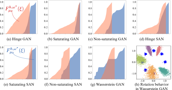
Figure 6: (a)-(g) Estimated cumulative density function at 5,000 iterations. Separability is satisfied in other GANs and SANs. In contrast, the discriminator does not satisfy separability in Wasserstein GAN. (h) Data samples and generated samples during training with Wasserstein GAN. Different colors represent different iterations (2,000, 4,000,$\ldots$, 10,000). Rotational behavior is observed.

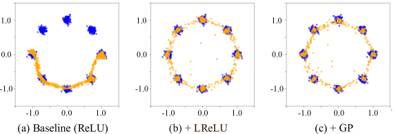
Figure 7: Effects of techniques to induce injectivity. The use of LReLU instead of ReLU and the addition of a GP to the maximization problem both improve the performance.

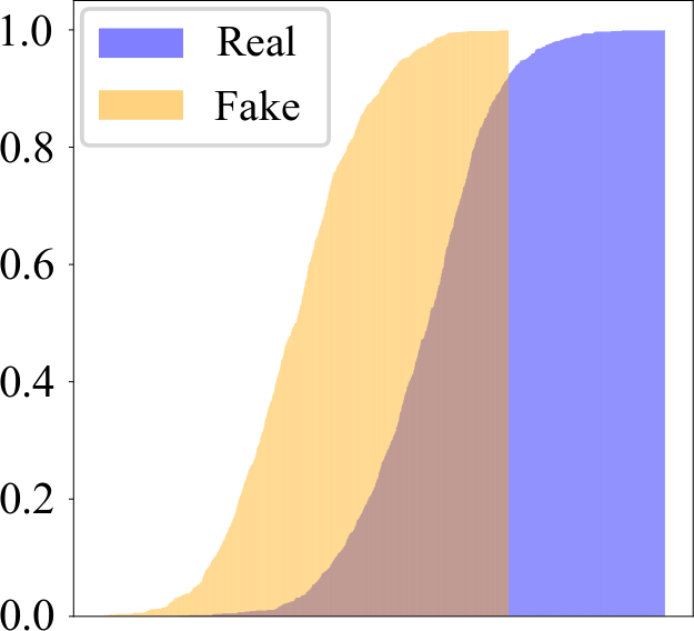
(a) Hinge SAN

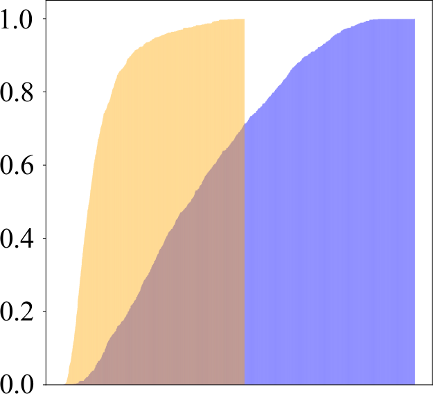
(b) Saturating SAN

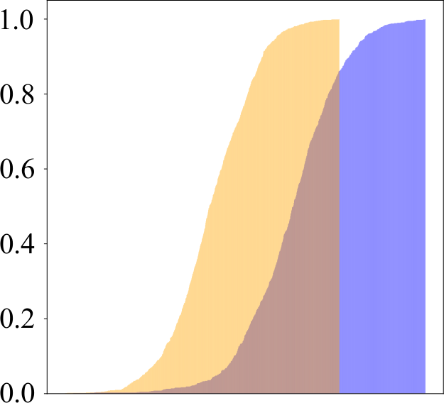
(c) Non-saturating SAN

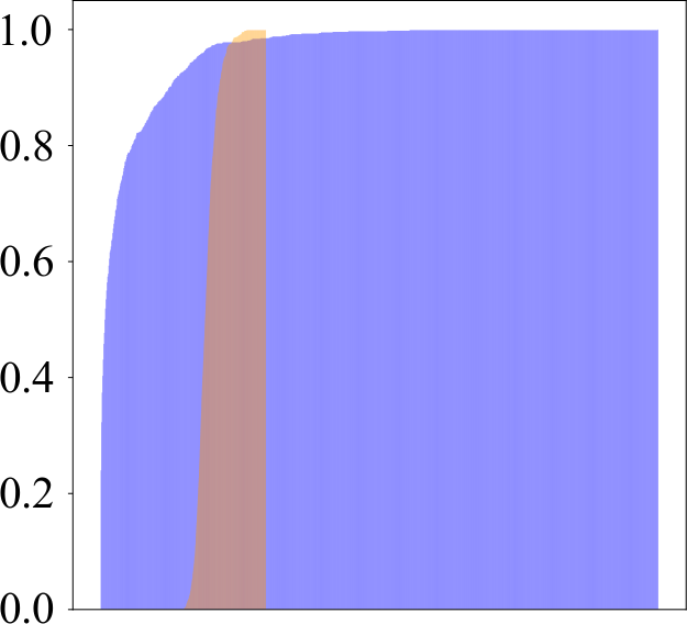
(d) Wasserstein GAN

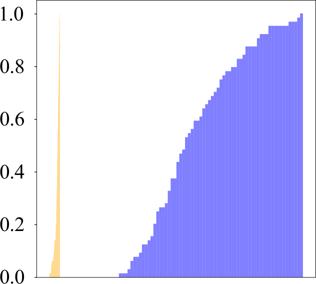
(e) Hinge GAN (ReLU)

Figure 8: Estimated cumulative density functions for the MNIST case. We follow the same procedure as in Fig. 5 to plot them. (a-c) Separability is satisfied by the SAN models. (d) In contrast, Wasserstein GAN does not satisfy the property, leading to bad generation results as in Figure II (d). (e) The use of ReLU in Hinge SAN does not destroy separability but leads to bad generation results due to the non-injectivity caused by the non-injective activation (see Fig. II (a)).

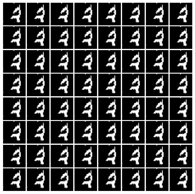
(a) Base line (ReLU)

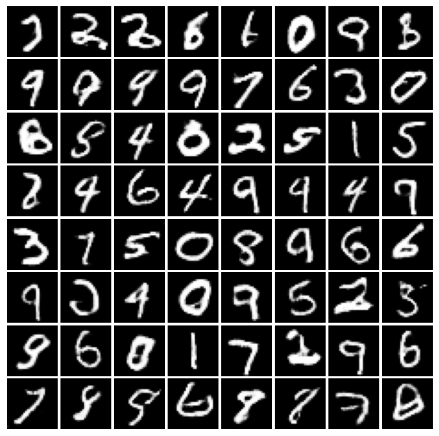
(b) +LReLU

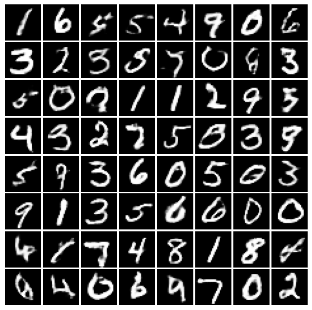
(c) +GP

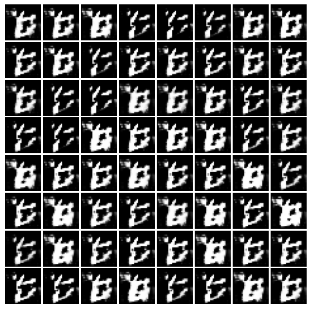
(d) Wasserstein GAN

Figure 9: (a-c) Effects of techniques to induce injectivity. (a) The use of ReLU leads to collape issue. (b) The use of LReLU instead of ReLU and (c) the addition of a GP to the maximization problem both improve the performance. (d) Generated results for Wasserstein GAN as a reference.

Appendix D Experimental Setup

D.1 Mixture of Gaussians

In Sec. 7.1 and Appx. E, we use the same experimental setup as below. For both the generator and the discriminator, we adopt simple architectures comprising fully connected layers by following the previous works (Mescheder et al., 2017; Nagarajan & Kolter, 2017; Sinha et al., 2020). We basically use leaky ReLU (LReLU) with a negative slope of $0.1$ for the discriminator.

D.2 Image Generation

DCGAN.

We borrow most parts of implementation from a public repository. Please refer to Tables 6 and 7 for details of the architectures. Spectral normalization is applied to the discriminator. We use Adam optimizer (Kingma & Ba, 2015) with betas of $(0.0,0.9)$ and an initial learning rate of 0.0002 for both the generator and discriminator. To convert GANs to SANs, we add two small modifications to the implementations. First, we apply a weight normalization instead of spectral normalization on the last linear layer of the discriminator, which makes its weight exactly on a hypersphere throughout the training. Next, we use the proposed objective functions for the maximization problems. We train the models for 2000 iterations with the minibatch size of 64. We run the training with three different seeds for all the models and report the mean and deviation values in Table 5.

Table 6: DCGAN architecture on CIFAR10.

Generator

Input: $z\in\mathbb{R}^{128}\sim\mathcal{N}(0,I)$

Deconv (4$\times$4, stride$=$1, channel$=$512), BN, ReLU

Deconv (4$\times$4, stride$=$2, channel$=$256), BN, ReLU

Deconv (4$\times$4, stride$=$2, channel$=$128), BN, ReLU

Deconv (4$\times$4, stride$=$2, channel$=$64), BN, ReLU

Deconv (4$\times$4, stride$=$1, channel$=$3), Tanh

Discriminator

Input: $x\in\mathbb{R}^{3\times 32\times 32}$

3$\times$3, stride$=1$, channel$=$64, LReLU

SNConv (4$\times$4, stride$=2$, channel$=$64), LReLU

SNConv (3$\times$3, stride$=$1, channel$=$128), LReLU

SNConv (4$\times$4, stride$=$2, channel$=$128), LReLU

SNConv (3$\times$3, stride$=$1, channel$=$256), LReLU

SNConv (4$\times$4, stride$=$2, channel$=$256), LReLU

SNConv (3$\times$3, stride$=$1, channel$=$512), LReLU

SNLinear

Table 7: DCGAN architecture on CelebA.

Generator

Input: $z\in\mathbb{R}^{128}\sim\mathcal{N}(0,I)$

Deconv (4$\times$4, stride$=$1, channel$=$512), BN, ReLU

Deconv (4$\times$4, stride$=$2, channel$=$256), BN, ReLU

Deconv (4$\times$4, stride$=$2, channel$=$128), BN, ReLU

Deconv (4$\times$4, stride$=$2, channel$=$64), BN, ReLU

Deconv (4$\times$4, stride$=$2, channel$=$32), BN, ReLU

Deconv (4$\times$4, stride$=$2, channel$=$3), Tanh

Discriminator

Input: $x\in\mathbb{R}^{3\times 128\times 28}$

3$\times$3, stride$=1$, channel$=$128, LReLU

SNConv ($4\times 4$, stride$=2$, channel$=$128), LReLU

SNConv (3$\times$3, stride$=$1, channel$=$256), LReLU

SNConv (4$\times$4, stride$=$2, channel$=$256), LReLU

SNConv (3$\times$3, stride$=$1, channel$=$512), LReLU

SNConv (4$\times$4, stride$=$2, channel$=$512), LReLU

SNConv (3$\times$3, stride$=$1, channel$=$1024), LReLU

SNLinear

BigGAN.

We use the authors’ PyTorch implementation to compare GANs and SANs in the setting of BigGAN on CIFAR10. We exactly follow the instructions in the repository to train the GAN in the class conditional generation task. Regarding the unconditional generation task, we simply replace the class embedding for the last linear layer with a single linear layer. Similarly to the DCGAN setting, we implement the SANs only by modifying the last linear layer of the discriminator and the maximization objective function. We run the training with three different seeds for respective cases and report the mean and deviation values in Table 5. Note that it has been reported that there are numerical gaps between the evaluation scores reported in the original paper and those obtained by reproduction with the PyTorch implementation (Song & Ermon, 2020).

StyleGAN-XL.

We use the official implementation to compare a GAN and a SAN in the setting of StyleGAN-XL. We follow the instructions in the repository to train StyleSAN-XL in the class conditional generation task. As in the DCGAN and BigGAN settings, we implement the SAN only by modifying the last linear layer of the discriminator and the maximization objective function. We train a $256\times 256$ generative model on top of the pretrained $128\times 128$ generative model in a progressive growing manner (Karras et al., 2018; Sauer et al., 2022). We set --kimg option to 11,000 according to an author’s comment in the repository. We then report the FID and IS calculated with the code provided in the repository.

Appendix E Investigation of Separability and Injectivity

E.1 Mixture of Gaussians

We visualize the generated samples mainly to confirm that the generator measures cover all the modes of the eight Gaussians. In addition, we plot the cumulative density functions of ${\mathcal{S}}^{h}I_{\mu_{0}}(\cdot,\omega)$ and ${\mathcal{S}}^{h}I_{\mu_{\theta}}(\cdot,\omega)$ to verify separability. As shown in Fig. 6, the cumulative density function for the generator measures trained with Wasserstein GAN does not satisfy separability, whereas the generator measures trained with other GAN losses satisfy this property. This may cause Wasserstein GAN’s rotation behavior, as seen in Fig. 6-(h).

To investigate the effect of injectivity on the training results, we train Hinge GAN using a discriminator with ReLU as a baseline. We apply two techniques to induce injectivity: (1) the use of LReLU and (2) the addition of a GP to the discriminator’s maximization problem. As shown in Fig. 7, with either of these techniques, the training is improved and mode collapse does not occur.

E.2 Vision Datasets

We extend the experiment in Appx. E.1 to MNIST (LeCun et al., 1998) to investigate injectivity and separability on vision datasets. First, we train SANs with various objective functions and Wasserstein GAN on MNIST. We adopt DCGAN architectures and apply spectral normalization to the discriminator. As in Appx. E.1, we plot the cumulative density function for the generator measures trained with various objective functions in Fig. 8. The trained generator measures empirically satisfy separability except for the case of Wasserstein GAN, which is a similar tendency to the case of MoG. Furthermore, we conducted ablation study regarding the technique inducing injectivity by following Appx. E.1. We train Hinge SAN using a discriminator with ReLU as a baseline. We compare this baseline with two cases: (1) the use of LReLU and (2) the addition of a GP to the discriminator’s objective function. We visualize the generated samples for the cases in Figs. 9 (a)-(c). We observe the generator trained with the ReLU-based discriminator suffers from the mode collapse issue. In contrast, the techniques inducing injectivity mitigate the issue and lead to reasonable generation results. As a reference, we put the generation result from a generator that is trained with a LReLU-based discriminator and Wasserstein GAN in Fig. 9 (d). The generated samples are completely corrupted. Note that the discriminator with ReLU satisfies separability as in Fig. 8 (e). It suggests that the deterioration in Hinge SAN with the ReLU-based discriminator (Fig. 9 (a)) and that in the Wasserstein GAN model (Fig. 9 (d)) are triggered by different causes, i.e., from non-injectivity and non-separability, respectively.

Appendix F Generated Samples

We show images generated by GANs and SANs in Figs. 10, 11, 12 and 8.

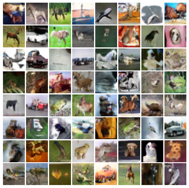
(a) Saturating GAN

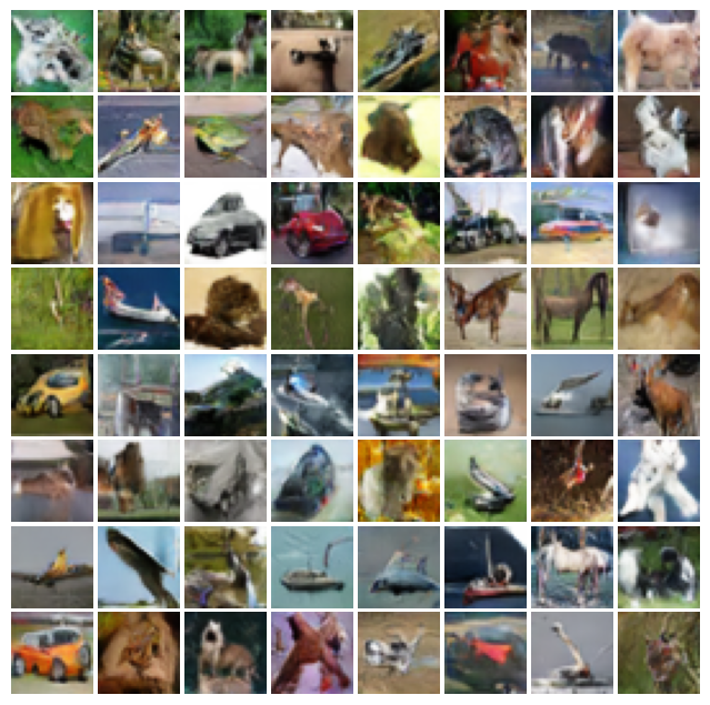
(b) Saturating SAN

Figure 10: Generated samples from DCGAN trained on CIFAR10.

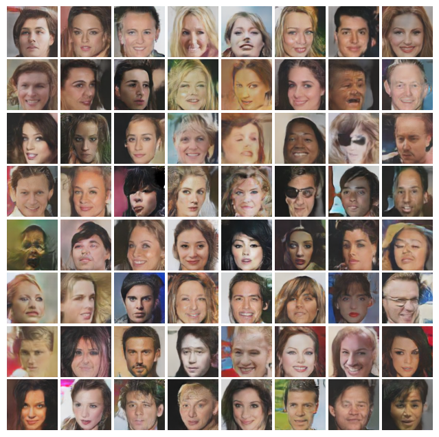
(a) Non-saturating GAN

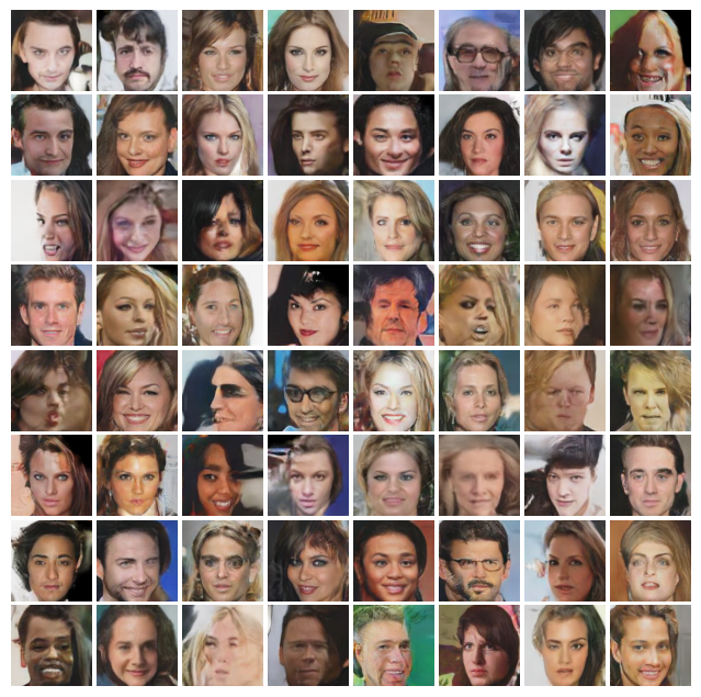
(b) Non-saturating SAN

Figure 11: Generated samples from DCGAN trained on CelebA (128$\times$128).

(a) Hinge GAN (unconditional)

(b) Hinge SAN (unconditional)

(c) Hinge GAN (conditional)

(d) Hinge SAN (conditional)

Figure 12: Generated samples from BigGAN trained on CIFAR10.

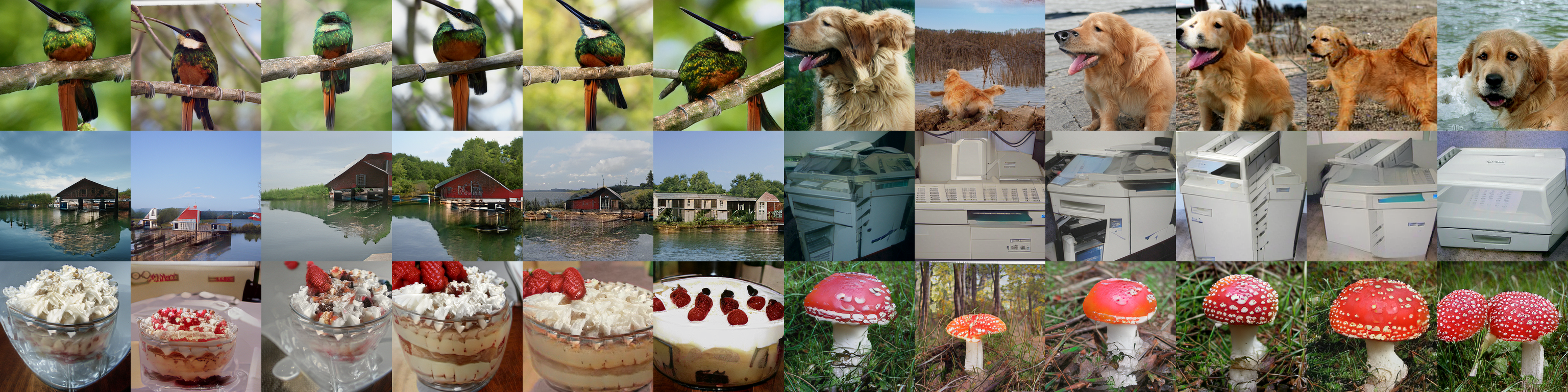
(a) StyleGAN-XL

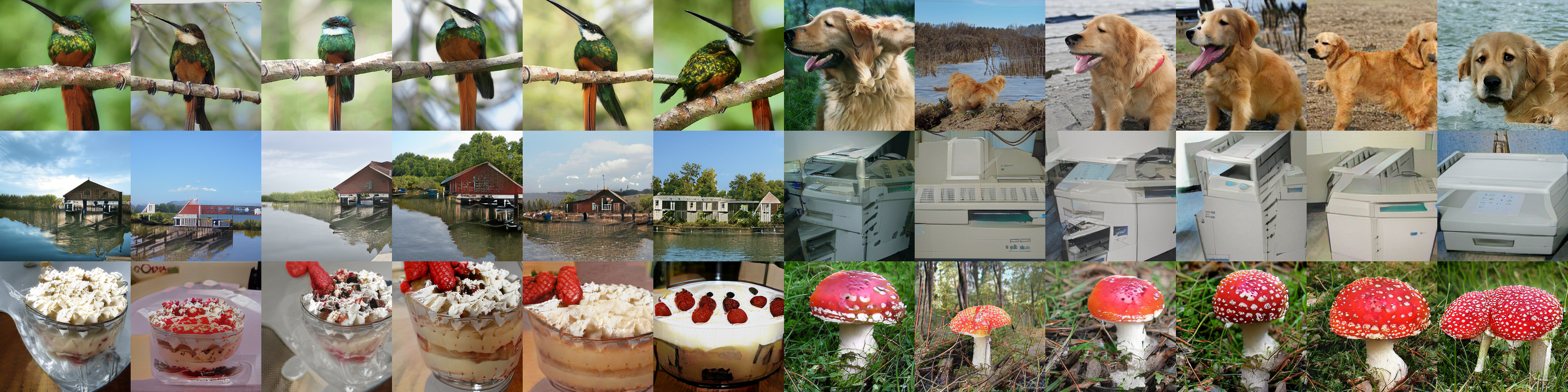
(b) StyleSAN-XL

Figure 13: Generated samples from StyleGAN-XLand StyleSAN-XL trained on ImageNet.

References

- Arjovsky et al. (2017) Martin Arjovsky, Soumith Chintala, and Léon Bottou. Wasserstein GAN. arXiv preprint arXiv:1701.07875, 2017.
- Behrmann et al. (2019) Jens Behrmann, Will Grathwohl, Ricky TQ Chen, David Duvenaud, and Jörn-Henrik Jacobsen. Invertible residual networks. In Proc. International Conference on Machine Learning (ICML), pp. 573–582, 2019.
- Berard et al. (2020) Hugo Berard, Gauthier Gidel, Amjad Almahairi, Pascal Vincent, and Simon Lacoste-Julien. A closer look at the optimization landscapes of generative adversarial networks. In Proc. International Conference on Learning Representation (ICLR), 2020.
- Bonneel et al. (2015) Nicolas Bonneel, Julien Rabin, Gabriel Peyré, and Hanspeter Pfister. Sliced and radon Wasserstein barycenters of measures. Journal of Mathematical Imaging and Vision, 51(1):22–45, 2015.
- Brock et al. (2019) Andrew Brock, Jeff Donahue, and Karen Simonyan. Large scale gan training for high fidelity natural image synthesis. In Proc. International Conference on Learning Representation (ICLR), 2019.
- Chen et al. (2022) Xiongjie Chen, Yongxin Yang, and Yunpeng Li. Augmented sliced wasserstein distances. In Proc. International Conference on Learning Representation (ICLR), 2022.
- Chu et al. (2020) Casey Chu, Kentaro Minami, and Kenji Fukumizu. Smoothness and stability in GANs. In Proc. International Conference on Learning Representation (ICLR), 2020.
- Deshpande et al. (2019) Ishan Deshpande, Yuan-Ting Hu, Ruoyu Sun, Ayis Pyrros, Nasir Siddiqui, Sanmi Koyejo, Zhizhen Zhao, David Forsyth, and Alexander G Schwing. Max-sliced Wasserstein distance and its use for GANs. In Proc. IEEE/CVF Conference on Computer Vision and Pattern Recognition (CVPR), pp. 10648–10656, 2019.
- Donahue et al. (2019) Chris Donahue, Julian McAuley, and Miller Puckette. Adversarial audio synthesis. In Proc. International Conference on Learning Representation (ICLR), 2019.
- Farnia & Ozdaglar (2020) Farzan Farnia and Asuman Ozdaglar. Do GANs always have nash equilibria? In Proc. International Conference on Machine Learning (ICML), pp. 3029–3039, 2020.
- Fiez et al. (2022) Tanner Fiez, Chi Jin, Praneeth Netrapalli, and Lillian J Ratliff. Minimax optimization with smooth algorithmic adversaries. In Proc. International Conference on Learning Representation (ICLR), 2022.
- Goodfellow et al. (2014) Ian Goodfellow, Jean Pouget-Abadie, Mehdi Mirza, Bing Xu, David Warde-Farley, Sherjil Ozair, Aaron Courville, and Yoshua Bengio. Generative adversarial nets. In Proc. Advances in Neural Information Processing Systems (NeurIPS), pp. 2672–2680, 2014.
- Gulrajani et al. (2017) Ishaan Gulrajani, Faruk Ahmed, Martin Arjovsky, Vincent Dumoulin, and Aaron C Courville. Improved training of Wasserstein GANs. In Proc. Advances in Neural Information Processing Systems (NeurIPS), pp. 5767–5777, 2017.
- Hao et al. (2021) Zekun Hao, Arun Mallya, Serge Belongie, and Ming-Yu Liu. GANcraft: Unsupervised 3d neural rendering of minecraft worlds. In Proc. IEEE/CVF International Conference on Computer Vision (ICCV), pp. 14072–14082, 2021.
- Helgason (2011) Sigurdur Helgason. The Radon transform on Rn. In Integral Geometry and Radon Transforms, pp. 1–62. Springer, 2011.
- Higgins et al. (2017) Irina Higgins, Loic Matthey, Arka Pal, Christopher Burgess, Xavier Glorot, Matthew Botvinick, Shakir Mohamed, and Alexander Lerchner. beta-VAE: Learning basic visual concepts with a constrained variational framework. In Proc. International Conference on Learning Representation (ICLR), 2017.
- Ho et al. (2020) Jonathan Ho, Ajay Jain, and Pieter Abbeel. Denoising diffusion probabilistic models. In Proc. Advances in Neural Information Processing Systems (NeurIPS), pp. 6840–6851, 2020.
- Jordan et al. (1999) Michael I Jordan, Zoubin Ghahramani, Tommi S Jaakkola, and Lawrence K Saul. An introduction to variational methods for graphical models. Machine Learning, 37(2):183–233, 1999.
- Karami et al. (2019) Mahdi Karami, Dale Schuurmans, Jascha Sohl-Dickstein, Laurent Dinh, and Daniel Duckworth. Invertible convolutional flow. In Proc. Advances in Neural Information Processing Systems (NeurIPS), volume 32, 2019.
- Karras et al. (2018) Tero Karras, Timo Aila, Samuli Laine, and Jaakko Lehtinen. Progressive growing of gans for improved quality, stability, and variation. In Proc. International Conference on Learning Representation (ICLR), 2018.
- Karras et al. (2019) Tero Karras, Samuli Laine, and Timo Aila. A style-based generator architecture for generative adversarial networks. In Proc. IEEE/CVF Conference on Computer Vision and Pattern Recognition (CVPR), pp. 4401–4410, 2019.
- Karras et al. (2021) Tero Karras, Miika Aittala, Samuli Laine, Erik Härkönen, Janne Hellsten, Jaakko Lehtinen, and Timo Aila. Alias-free generative adversarial networks. In Proc. Advances in Neural Information Processing Systems (NeurIPS), 2021.
- Kingma & Ba (2015) Diederik P Kingma and Jimmy Ba. Adam: A method for stochastic optimization. In Proc. International Conference on Learning Representation (ICLR), 2015.
- Kingma & Welling (2014) Diederik P Kingma and Max Welling. Auto-encoding variational Bayes. In Proc. International Conference on Learning Representation (ICLR), 2014.
- Kolouri et al. (2019) Soheil Kolouri, Kimia Nadjahi, Umut Simsekli, Roland Badeau, and Gustavo Rohde. Generalized sliced Wasserstein distances. In Proc. Advances in Neural Information Processing Systems (NeurIPS), volume 32, 2019.
- Kong et al. (2020) Jungil Kong, Jaehyeon Kim, and Jaekyoung Bae. HiFi-gan: Generative adversarial networks for efficient and high fidelity speech synthesis. In Proc. Advances in Neural Information Processing Systems (NeurIPS), volume 33, pp. 17022–17033, 2020.
- Krizhevsky et al. (2009) Alex Krizhevsky, Geoffrey Hinton, et al. Learning multiple layers of features from tiny images. 2009.
- Kumar et al. (2019) Kundan Kumar, Rithesh Kumar, Thibault de Boissiere, Lucas Gestin, Wei Zhen Teoh, Jose Sotelo, Alexandre de Brébisson, Yoshua Bengio, and Aaron C Courville. MelGAN: Generative adversarial networks for conditional waveform synthesis. In Proc. Advances in Neural Information Processing Systems (NeurIPS), volume 32, 2019.
- LeCun et al. (1998) Yann LeCun, Léon Bottou, Yoshua Bengio, and Patrick Haffner. Gradient-based learning applied to document recognition. Proc. IEEE, 86(11):2278–2324, 1998.
- Lim & Ye (2017) Jae Hyun Lim and Jong Chul Ye. Geometric gan. arXiv preprint arXiv:1705.02894, 2017.
- Lin et al. (2021) Zinan Lin, Vyas Sekar, and Giulia Fanti. Why spectral normalization stabilizes GANs: Analysis and improvements. volume 34, pp. 9625–9638, 2021.
- Liu et al. (2015) Ziwei Liu, Ping Luo, Xiaogang Wang, and Xiaoou Tang. Deep learning face attributes in the wild. In Proc. IEEE Conference on Computer Vision and Pattern Recognition (CVPR), pp. 3730–3738, 2015.
- Mescheder et al. (2017) Lars Mescheder, Sebastian Nowozin, and Andreas Geiger. The numerics of gans. In Proc. Advances in Neural Information Processing Systems (NeurIPS), volume 30, 2017.
- Mescheder et al. (2018) Lars Mescheder, Andreas Geiger, and Sebastian Nowozin. Which training methods for GANs do actually converge? In Proc. International Conference on Machine Learning (ICML), pp. 3481–3490, 2018.
- Milgrom & Segal (2002) Paul Milgrom and Ilya Segal. Envelope theorems for arbitrary choice sets. Econometrica, 70(2):583–601, 2002.
- Miyato & Koyama (2018) Takeru Miyato and Masanori Koyama. cgans with projection discriminator. In Proc. International Conference on Learning Representation (ICLR), 2018.
- Miyato et al. (2018) Takeru Miyato, Toshiki Kataoka, Masanori Koyama, and Yuichi Yoshida. Spectral normalization for generative adversarial networks. In Proc. International Conference on Learning Representation (ICLR), 2018.
- Müller (1997) Alfred Müller. Integral probability metrics and their generating classes of functions. Advances in Applied Probability, 29(2):429–443, 1997.
- Nagarajan & Kolter (2017) Vaishnavh Nagarajan and J Zico Kolter. Gradient descent GAN optimization is locally stable. In Proc. Advances in Neural Information Processing Systems (NeurIPS), volume 30, 2017.
- Natterer (2001) Frank Natterer. The mathematics of computerized tomography. SIAM, 2001.
- Nguyen et al. (2021) Khai Nguyen, Nhat Ho, Tung Pham, and Hung Bui. Distributional sliced-Wasserstein and applications to generative modeling. In Proc. International Conference on Learning Representation (ICLR), 2021.
- Nichol & Dhariwal (2021) Alexander Quinn Nichol and Prafulla Dhariwal. Improved denoising diffusion probabilistic models. In Proc. International Conference on Machine Learning (ICML), pp. 8162–8171. PMLR, 2021.
- Nowozin et al. (2016) Sebastian Nowozin, Botond Cseke, and Ryota Tomioka. f-GAN: Training generative neural samplers using variational divergence minimization. In D. Lee, M. Sugiyama, U. Luxburg, I. Guyon, and R. Garnett (eds.), Proc. Advances in Neural Information Processing Systems (NeurIPS), volume 29, 2016.
- Radford et al. (2016) Alec Radford, Luke Metz, and Soumith Chintala. Unsupervised representation learning with deep convolutional generative adversarial networks. In Proc. International Conference on Learning Representation (ICLR), 2016.
- Rezende & Mohamed (2015) Danilo Jimenez Rezende and Shakir Mohamed. Variational inference with normalizing flows. In Proc. International Conference on Machine Learning (ICML), pp. 1530–1538, 2015.
- Russakovsky et al. (2015) Olga Russakovsky, Jia Deng, Hao Su, Jonathan Krause, Sanjeev Satheesh, Sean Ma, Zhiheng Huang, Andrej Karpathy, Aditya Khosla, Michael Bernstein, et al. Imagenet large scale visual recognition challenge. International journal of computer vision, 115:211–252, 2015.
- Salimans et al. (2016) Tim Salimans, Ian Goodfellow, Wojciech Zaremba, Vicki Cheung, Alec Radford, and Xi Chen. Improved techniques for training GANs. In Proc. Advances in Neural Information Processing Systems (NeurIPS), volume 29, 2016.
- Sanjabi et al. (2018) Maziar Sanjabi, Jimmy Ba, Meisam Razaviyayn, and Jason D Lee. On the convergence and robustness of training gans with regularized optimal transport. In Proc. International Conference on Machine Learning (ICML), volume 31, 2018.
- Sauer et al. (2022) Axel Sauer, Katja Schwarz, and Andreas Geiger. Stylegan-xl: Scaling stylegan to large diverse datasets. In ACM SIGGRAPH 2022 conference proceedings, pp. 1–10, 2022.
- Sinha et al. (2020) Samarth Sinha, Anirudh Goyal, Colin Raffel, and Augustus Odena. Top-k training of GANs: Improving generators by making critics less critical. In Proc. Advances in Neural Information Processing Systems (NeurIPS), 2020.
- Song & Ermon (2020) Jiaming Song and Stefano Ermon. Bridging the gap between f-gans and wasserstein gans. In Proc. International Conference on Machine Learning (ICML), pp. 9078–9087, 2020.
- Song et al. (2020) Jiaming Song, Chenlin Meng, and Stefano Ermon. Denoising diffusion implicit models. In Proc. International Conference on Learning Representation (ICLR), 2020.
- Song et al. (2019) Yang Song, Chenlin Meng, and Stefano Ermon. Mintnet: Building invertible neural networks with masked convolutions. In Proc. Advances in Neural Information Processing Systems (NeurIPS), volume 32, 2019.
- Srivastava et al. (2017) Akash Srivastava, Lazar Valkov, Chris Russell, Michael U Gutmann, and Charles Sutton. VEEGAN: Reducing mode collapse in gans using implicit variational learning. In Proc. Advances in Neural Information Processing Systems (NeurIPS), volume 30, 2017.
- Tabak & Turner (2013) Esteban G Tabak and Cristina V Turner. A family of nonparametric density estimation algorithms. Communications on Pure and Applied Mathematics, 66(2):145–164, 2013.
- Tabak & Vanden-Eijnden (2010) Esteban G Tabak and Eric Vanden-Eijnden. Density estimation by dual ascent of the log-likelihood. Communications in Mathematical Sciences, 8(1):217–233, 2010.
- Takida et al. (2022) Yuhta Takida, Takashi Shibuya, WeiHsiang Liao, Chieh-Hsin Lai, Junki Ohmura, Toshimitsu Uesaka, Naoki Murata, Takahashi Shusuke, Toshiyuki Kumakura, and Yuki Mitsufuji. SQ-VAE: Variational Bayes on discrete representation with self-annealed stochastic quantization. In Proc. International Conference on Machine Learning (ICML), 2022.
- Tulyakov et al. (2018) Sergey Tulyakov, Ming-Yu Liu, Xiaodong Yang, and Jan Kautz. MoCoGAN: Decomposing motion and content for video generation. In Proc. IEEE Conference on Computer Vision and Pattern Recognition (CVPR), pp. 1526–1535, 2018.
- Villani (2009) Cédric Villani. Optimal transport: old and new, volume 338. Springer, 2009.
- Xu et al. (2020) Kun Xu, Chongxuan Li, Jun Zhu, and Bo Zhang. Understanding and stabilizing GANs’ training dynamics with control theory. In Proc. International Conference on Machine Learning (ICML), pp. 10566–10575, 2020.
- Zhang et al. (2019) Han Zhang, Ian Goodfellow, Dimitris Metaxas, and Augustus Odena. Self-attention generative adversarial networks. In Proc. International Conference on Machine Learning (ICML), pp. 7354–7363, 2019.
- Zhao et al. (2019) Shengjia Zhao, Jiaming Song, and Stefano Ermon. InfoVAE: Balancing learning and inference in variational autoencoders. In Proc. AAAI Conference on Artificial Intelligence (AAAI), pp. 5885–5892, 2019.