Cosmic growth rate measurements from Tully-Fisher peculiar velocities

Abstract

Peculiar velocities are an important probe of the growth rate of structure in the Universe, directly measuring the effects of gravity on the largest scales and thereby providing a test for theories of gravity. Complete peculiar velocity datasets comprise both galaxy redshifts and redshift-independent distance measures, estimated by methods such as the Tully-Fisher relation. Traditionally, the Tully-Fisher relation is first calibrated using distance indicators such as Cepheid variables in a small sample of galaxies; the calibrated relation is then used to determine peculiar velocities. In this analysis, we employ a one-step Bayesian method to simultaneously determine the parameters of the Tully-Fisher relation and the peculiar velocity field. We have also generalised the Tully-Fisher relation by allowing for a curvature at the bright end. We design a mock survey to emulate the Cosmicflows-4 (CF4) peculiar velocity dataset. We then apply our method to the CF4 data to obtain new constraints for the growth rate of structure parameter ($\beta=0.40\pm 0.07$), the residual bulk flow ($\mathbf{V}_{\textrm{ext}}=$[69$\pm$15,$-$158$\pm$9,14$\pm$7] km$~{}s^{-1}$ in Supergalactic coordinates), and the parameters for a Tully-Fisher relation with curvature. We obtain an estimate for the product of the growth rate and mass fluctuation amplitude $f\sigma_{8}=0.40\pm 0.07$. We combine this measurement of $f\sigma_{8}$ with those of other galaxy redshift surveys to fit the growth index $\gamma$. Assuming cosmological parameters from the latest Planck CMB results, we find that $\gamma>6/11$ is favoured. We plan to use this improved method for recovering peculiar velocities on the large new samples of Tully-Fisher data from surveys such as WALLABY, resulting in more precise growth rate measurements at low redshifts.

1 Introduction

The continuous action of gravity over the history of structure growth in the Universe is reflected by the present-day velocities of its constituents. Peculiar velocities, the motions of galaxies on top of the overall expansion of the Universe, thus offer a powerful method to test General Relativity (GR) via the time evolution of the growth rate of structure. This probe is sensitive to very small deviations from GR because small differences in galaxy acceleration are amplified over time (Strauss & Willick, 1995). However, much more precise measurements of the growth rate than currently exist are required to distinguish GR from plausible alternatives.

In the linear regime, the peculiar velocity field is directly related to the density field of galaxies through the peculiar acceleration (Strauss & Willick, 1995),

$$\mathbf{v}(\mathbf{r})=\frac{H_{0}\beta}{4\pi}\int\textrm{d}^{3}\mathbf{r^{\prime}}\frac{\delta_{g}(\mathbf{r^{\prime}})(\mathbf{r^{\prime}}-\mathbf{r})}{|\mathbf{r^{\prime}}-\mathbf{r}|^{3}},$$ (1)

where $\beta$ is the cosmology- and bias-dependent parameter that relates the two quantities. Simultaneous measurements of the peculiar velocity field $\mathbf{v}(\mathbf{r})$ and the galaxy density field $\delta_{g}(\mathbf{r})$ thus allow us to constrain the parameter $\beta$.

In order to study peculiar velocities, measures of galaxy distance that are independent of redshift are needed. One option is a two-step approach, in which a small number of calibrators may be used to fit a distance-indicator relation in a first step, followed by fitting the velocity field parameters in a second step. This method works because redshifts are quite precise indicators of distance at sufficiently large distances that the Hubble velocity is much greater than typical peculiar velocities. However, this approach inflates the scatter around the distance-indicator relation by ignoring the peculiar velocities.

An alternative approach, advocated here, uses a Bayesian forward-modelling methodology in which the parameters of the velocity field model and of the distance-indicator relation are inferred jointly in one step. This method treats the parameters of the model and the relation as continuous and free, and generates predictions of the observables given their values. It then finds the best fit between the observed data and the predicted observables, yielding the corresponding parameter estimates and their (correlated) uncertainties.

This methodology is derived from Saglia et al. (2001) and Colless et al. (2001), who used 3D Gaussians to fit the Fundamental Plane distance indicator for early-type galaxies. Howlett et al. (2022) also built upon this approach, while Said et al. (2020) used it with forward-modelling. Willick et al. (1997) also used a forward-modelling approach to Tully-Fisher data, but with limited success at the time. Here, we adapt the methodology described in Said et al. (2020) and apply it for the first time to the Tully-Fisher (TF) relation, a distance indicator for late-type (rotation-dominated, spiral) galaxies, obtaining both peculiar velocities for individual galaxies and new constraints on the cosmological parameter $\beta$.

The paper is organised as follows. In Section 2 we describe the CF4 data and the model used to fit and simulate it, including a non-linear Tully-Fisher relation (Section 2.1), a non-constant scatter model (Section 2.2), and the data selection criteria (Section 2.3). The sky coverage of CF4 data is shown in Fig. 2 and redshift coverage in Fig. 3. In Section 3 we describe the selection function for the CF4 data. In Section 4 we describe the methodology used to simultaneously fit the Tully-Fisher relation and the cosmological model to the data. In Section 5 we summarise our simulation framework, including the models used (Section 5.1), the sample selection criteria (Section 5.2), the procedure for generating mocks (Section 5.3), and the results of testing our method on the simulated data (Section 5). In Section 6 we present the results of our analysis applied to the CF4 catalogue; the constraints on the parameters of our model are shown in Fig. 10. In Section 7 we discuss prospects for future applications of this method to WALLABY data. In Section 8 we state our conclusions.

Unless otherwise noted, we assume a flat $\Lambda$CDM cosmology with $\Omega_{m}=0.315$, as favoured by Aghanim et al. (2020), and $H_{0}=100h$ $\mathrm{kms^{-1}Mpc^{-1}}$.

2 Tully-Fisher relation

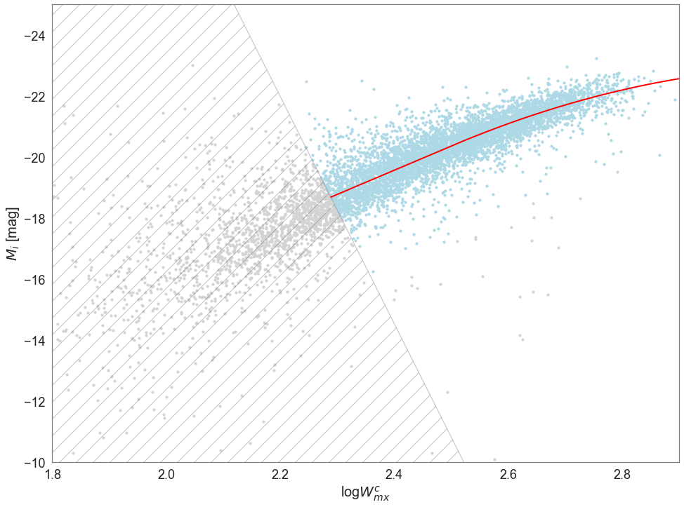
Figure 1: The Tully-Fisher relation for the ALFALFA subset of CF4, where observed galaxy redshifts were corrected by removing peculiar velocities implied by the 2M++ peculiar velocity model. Galaxies within the hashed grey region are excluded (see Section 2.3). The curved Tully-Fisher model fit is shown in red.

At large radii, spiral galaxies tend to have a flat rotation curves characterised by their maximum rotation velocity $v_{\textrm{rot}}$. They show a tight correlation between $v_{\textrm{rot}}$ and their intrinsic luminosity $L$, which is called the Tully-Fisher relation (Tully & Fisher, 1977). Simply stated, brighter spirals rotate faster. This relation is well-modelled by a power law (Strauss & Willick, 1995),

$$L(v_{\textrm{rot}})\propto v_{\textrm{rot}}^{\alpha}~{}.$$ (2)

Astronomers conventionally use absolute magnitudes rather than luminosities, so the Tully-Fisher relationship can be written as

$$M=a(\log{2v_{\textrm{rot}}}-2.5)+b$$ (3)

where $M=\textrm{const}-2.5\log{L}$ is the absolute magnitude of the galaxy, $v_{\textrm{rot}}$ is the rotation velocity in the ‘flat’ part of the rotation curve, and $a$ and $b$ are the slope and zero-point of the Tully-Fisher relation. The distance-dependent observed quantity is the apparent magnitude $m$, which is related to the absolute magnitude by

$$m=M+5\log{r}\equiv M+\mu(r)$$ (4)

where $r$ is the luminosity distance to the galaxy and $\mu(r)$ is a convenient logarithmic measure known as the distance modulus.

Rotation velocities $v_{\textrm{rot}}$ are closely related to the inclination-corrected H I line widths at 50% mean flux, $W_{\textrm{m50}}$. The procedure for this adjustment is explained by Courtois et al. (2009). We adopt their notation of $W_{\textrm{mx}}$ to represent the quantity that approximates $2v_{\textrm{rot}}\sin{i}$, where $i$ is the galaxy inclination. Throughout this paper, we will use $W_{\textrm{mx}}^{c}=W_{\textrm{mx}}/\sin{i}$ in place of $2v_{\textrm{rot}}$ as the independent variable of the Tully-Fisher relation, and we will call $W_{\textrm{mx}}^{c}$ the ‘velocity width’.

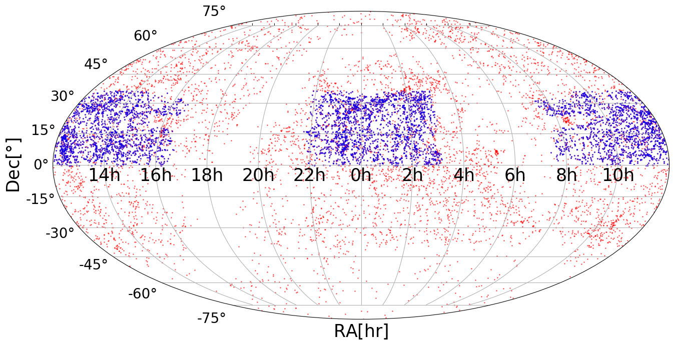
Figure 2: Sky coverage of the CF4 data (red) and the ALFALFA subset (blue). While the full CF4 catalogue covers the whole sky, ALFALFA is limited to two continuous regions in the Arecibo Spring and Fall skies.

Figure 3: Redshift distributions of the full CF4 sample (red) and the ALFALFA galaxies in CF4 (blue).

The Cosmicflows-4 (CF4) Tully-Fisher catalogue (Kourkchi et al., 2020b) is based on heterogeneous datasets and contains 10,737 galaxies. It is currently the largest full-sky catalogue of galaxies with Tully-Fisher distances and peculiar velocities. The Tully-Fisher distance indicator uses, as the distance-independent quantity, the rotation velocity of spiral galaxies, for which it takes as a proxy the broadening of the emitted neutral hydrogen (H I) line. The distance-dependent quantity is the galaxy luminosity, based on the photometric magnitude. These measurements, along with redshifts, comprise the Tully-Fisher dataset. The H I data is taken primarily from the All Digital H I (ADHI) catalogue (Courtois et al., 2009), which itself is composed mainly of good-quality H I data from the ALFALFA survey (Haynes et al., 2018).

Conventionally, the Tully-Fisher relationship is characterised by a simple model: a linear relationship between absolute magnitude and velocity width with a constant RMS scatter in absolute magnitude. However, since this is an empirical model, we should re-evaluate the legitimacy of using this simple model in the context of new datasets covering regions of parameter space that have not previously been included in calibrations. This can involve making modifications to the empirical model and/or introducing upper/lower limits to the regions where the relationship holds.

In this work, we take an agnostic approach to determining an appropriate Tully-Fisher model. To obtain a base Tully-Fisher dataset that we will use for developing our model, we use the velocity widths provided by CF4, in which observed linewidths at 50% average H I flux have been adjusted to approximate twice the rotation velocity after deprojection using the inclinations (Kourkchi et al., 2020b). We estimate distances $r$ from observed redshifts $z$ (in the CMB frame) using the following relation:

$$1+z=\Big{(}1+\frac{H_{0}r}{c}\Big{)}\Big{(}1+\frac{u(z,RA,Dec)}{c}\Big{)}$$ (5)

where $u(z,RA,Dec)$ is the line-of-sight peculiar velocity predicted by the model derived from the 2M++ redshift compilation (Carr et al., 2022). Using these distance estimates, we convert the measured apparent magnitudes to absolute magnitudes. The resulting velocity widths and absolute magnitudes are plotted in Fig. 1.

The 2M++ velocity field reconstruction was chosen because other studies have found it to be the most accurate available representation; for example, Peterson et al. (2022) found it to be optimal when make peculiar velocity corrections to redshifts. In any case, velocities fields from most reconstructions methods agree with each other within the error margins of this analysis. However, the choice of reconstruction may require attention in the future with WALLABY.

2.1 Tully-Fisher non-linearity

In Kourkchi et al. (2020a), a quadratic term was added to the Tully-Fisher relation for values of $\log{W_{\textrm{m50}}^{c}}>2.5$, which results in a downward curvature of the relation at the bright end. Kourkchi et al. chose to fix the break-point from the linear relation at $\log{W_{m50}}=2.5$, but we allow the break-point to be a free parameter. This model has the form

$$M=\begin{cases}aw+b&w<d\\ aw+b+a_{2}w^{2}&w\geq d\\ \end{cases}$$ (6)

where $w\equiv\log{W_{\textrm{mx}}^{c}}-2.5$.

To cover our bases, we also test the viability of a purely linear model. We fit each of these models to the CF4 data using orthogonal distance regression. Table 1 lists the parameters and the residual variance for each model. Even though it has the largest number of free parameters, we find the curved model is the best representation of the data, as it produces the lowest reduced $\chi^{2}$.

For this dataset, the curvature break-point is fixed at $d=0$ (corresponding to $\log{W_{\textrm{mx}}^{c}}>2.5$) as in Kourkchi et al. (2020a). In Section 7, $d$ is left to be a free parameter, as there is more than enough data to generate precise constraints on the fit parameters.

Table 1: Best-fit parameter values of curved and linear Tully-Fisher models for the CF4 sample.

Parameter	Value	Description
Curved model
$a$	$-$7.93$\pm$0.07	slope
$b$	$-$20.36$\pm$0.01 mag	intercept
$d$	0	curvature break-point
$a_{2}$	6.0$\pm$0.4	curvature coefficient
$\chi^{2}/(n-5)$	0.15	reduced $\chi^{2}$
Linear model
$a$	$-$8.23$\pm$0.06	slope
$b$	$-$20.259$\pm$0.009 mag	intercept
$\chi^{2}/(n-3)$	0.16	reduced $\chi^{2}$

2.2 Tully-Fisher intrinsic scatter model

In the calibration of the Tully-Fisher relation of the CF4 galaxies by Kourkchi et al. (2020a), a nonlinear model of the Tully-Fisher scatter was adopted (see their Fig.9). They found that the RMS scatter in absolute magnitude could be approximated by a quadratic relation in absolute magnitude. This model was determined using only the calibrator galaxies, a much smaller number than the full CF4 dataset, encompassing a narrower range of absolute magnitudes. We find it cannot be applied to this analysis, as the model gives unreasonable scatters for the brightest galaxies in our sample (the parabola reaches an inflection point before the end of our magnitude range). We thus seek a new model to approximate the Tully-Fisher scatter.

To guide us, we create an initial fit of a curved Tully-Fisher relation using only observational errors in the fit. We find the residuals of the data from this model vary linearly with velocity width or absolute magnitude: the trend is sufficiently represented by a linear relationship, and over-fitted by any higher-order polynomial. For the actual model, the residuals are calculated orthogonally from the Tully-Fisher relation and are allowed to vary linearly along the relation itself. Thus the scatter model takes the form of a linear function of $w$:

$$\sigma_{\textrm{TF}}=a_{\sigma}w+b_{\sigma}~{}.$$ (7)

Computation of $\sigma_{\textrm{TF}}$ itself requires prior knowledge of the Tully-Fisher parameters in order to determine the orthogonal direction. As a result, adopting this kind of model requires a few iterations of the method, with the Tully-Fisher parameters updated each time.

2.3 Data cuts

For fainter galaxies, where the velocity widths are lower, the data becomes increasingly scattered about the relation. The observational errors are also much greater. As a result, we found that including this data in our Tully-Fisher relation and scatter model resulted in poor fits and larger uncertainties in the parameters. We thus attempt to remove those galaxies from our fitting procedure by imposing a cut that is orthogonal to the Tully-Fisher relation—since we are doing an orthogonal regression, the reduced $\chi^{2}$ is calculated using the orthogonal residuals, and the cut must be orthogonal to the relation to avoid biasing these residuals. The placement of this cut along the relation should be such that the reduced $\chi^{2}$ is minimised, since we aim to strike a balance between improving the fit (reducing the RMS residuals) and keeping as much data as possible (maximising the sample size).

Because the slope of the orthogonal cut and the reduced $\chi^{2}$ (computed after the cut has been applied) both depend on the unknown Tully-Fisher parameters, the final determination of an orthogonal cut requires several iterations of cutting, fitting, and optimising. The scatter model as described in Section 2.2 is also updated in the course of these iterations. During this procedure, Tully-Fisher parameters are determined using orthogonal least squares regression. Fig. 4 shows the reduced $\chi^{2}$ values for a range of orthogonal cuts in the final iteration. The minimum (where $\log{W_{\textrm{mx}}^{c}}=2.3$ at the intersection with the Tully-Fisher relation) suggests an optimal cut that removes about 25% of the sample, and is shown in Fig. 1.

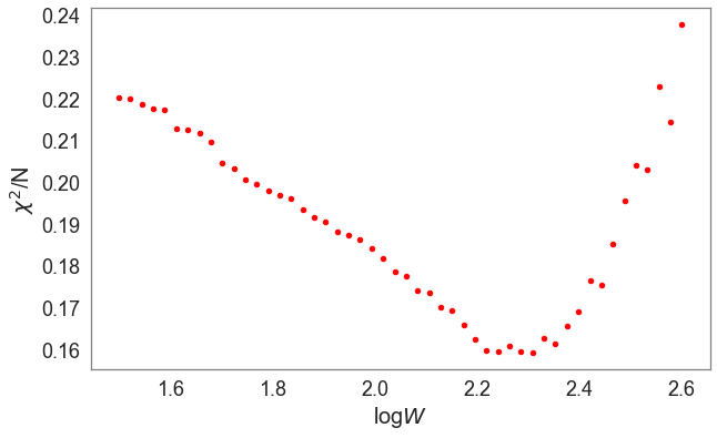
Figure 4: Reduced $\chi^{2}$ values of the Tully-Fisher model fit to the ALFALFA subset of CF4 data for a range of orthogonal cuts, in orthogonal units. The $x$–axis indicates the $\log{W_{\textrm{mx}}^{c}}$ value of the intersecting point with the Tully-Fisher relation. The plot shows the final iteration after repeatedly computing Tully-Fisher slopes and their orthogonal counterparts. The minimum occurs at $\log{W_{\textrm{mx}}^{c}}=2.3$.

2.4 Outliers

One important assumption of the scatter model is that at any given point along the Tully-Fisher relation, the residuals in absolute magnitude (or velocity width) have a Gaussian distribution. In fact, if we check this assumption by examining the distribution of the residuals in slices of absolute magnitude (or velocity width), we find they have overly-large wings and cannot be characterised by a pure Gaussian. If these outliers were indeed valid data points, this could break our simple assumption of Gaussian scatter and warrant a more complex model. However, a visual check of each misbehaving galaxy has revealed good reasons to remove a large portion of them from the sample; see Appendix B for a more detailed discussion on the removal of outliers from this dataset. Once the galaxies with readily identifiable issues are removed from the sample, we find the residuals are in fact adequately described by Gaussian distributions.

3 Selection function

The validity of statistical methods such as $\chi^{2}$ minimisation requires that objects in a sample be representative of the entire population of such objects. This is not true if there are observational selection criteria, such as a flux limit, since it is impossible for objects beyond this limit to belong to the sample. If all the selection criteria are well-defined, these selection biases can be compensated for and the observed sample can be readily related to a complete, volume-limited sample. To achieve this, we define a selection function $S_{n}$, for each galaxy $n$, as the fraction of the survey volume over which that galaxy, with its specific observational properties, can be observed given the selection criteria. The likelihood of finding a galaxy with these observed properties in a volume-limited sample can be obtained by calculating the intrinsic probability of these properties for arbitrary parameters of the Tully-Fisher relation, the velocity field model, and the Tully-Fisher scatter, and then weighting that probability by the inverse of the selection function $S_{n}$. This corresponds to replacing each galaxy with selection function $S_{n}$ by $1/S_{n}$ clones, to account for similar galaxies missed from the sample due to the selection criteria. The method assumes the observed sample is a selection-weighted fair sample from the underlying volume-limited population (this approximation fails if the selection function goes to zero for a significant subset of the underlying population).

In Said et al. (2020), the selection function is calculated as

$$S_{n}=\begin{cases}1&z_{n}^{\textrm{max}}\geq z_{\textrm{max}}\\ \frac{V_{n}^{\textrm{max}}-V(z_{\textrm{min}})}{V(z_{\textrm{max}})-V(z_{\textrm{min}})}&z_{\textrm{min}}<z_{n}^{\textrm{max}}<z_{\textrm{max}}\\ 0&z_{n}^{\textrm{max}}\leq z_{\textrm{min}}\end{cases}$$ (8)

where $z_{\textrm{min}}$ and $z_{\textrm{max}}$ are the upper and low redshift limits for the survey (effectively defining the underlying volume-limited sample) and $V(z_{\textrm{min}})$ and $V(z_{\textrm{max}})$ are the corresponding comoving volumes, while $z_{n}^{\rm max}$ is the maximum redshift at which the galaxy $n$ would be observed given the sample selection criteria and $V_{n}^{\rm max}$ is the corresponding volume.

4 Method

This section describes a Bayesian forward-modelling methodology (i.e. a method comparing observed quantities to ones predicted from a model) in which the parameters of the velocity field model and of the distance indicator relation are inferred jointly in one step. This methodology was originally developed by Willick et al. (1997) and first applied in the context of the problem of estimating distances for early-type galaxies from the Fundamental Plane relation by Saglia et al. (2001) and Colless et al. (2001). It has been extended and improved recently by Said et al. (2020) and Howlett et al. (2022) for application to the large Fundamental Plane datasets from the 6dFGS and SDSS surveys. The method can be generalised to incorporate any kind of redshift–distance measurements.

In this section, we present a straightforward modification of the methodology for Tully-Fisher distances. The free parameters of the model describe the Tully-Fisher relation ($a$, $b$, $a_{2}$, $d$, $a_{\sigma}$ and $b_{\sigma}$) and the peculiar velocity field (the scaling parameter $\beta$ and the residual bulk flow $\mathbf{V}_{\textrm{ext}}$), while the observed data are the Tully-Fisher observables ($m$ and $w\equiv\log{W_{\textrm{mx}}^{c}}-2.5$) and redshift ($z$). The peculiar velocity field parameters and Tully-Fisher parameters are fitted simultaneously, and the joint probability for the observable quantities at comoving location $\mathbf{r}$ is expressed as $P(m,w,z,\mathbf{r})$.

In this formulation, the true distance $r$ is the only non-observable quantity. Fortunately, it is possible to integrate out the distance-dependence, yielding the probability distribution of the Tully-Fisher observables of a galaxy given its redshift

$$P(w,m,z)=\int^{\infty}_{0}P(w,m,z,\mathbf{r})dr~{}.$$ (9)

The reason we are able to integrate the joint probability distributions over $r$ is that the Tully-Fisher observables and the redshift are coupled through their individual dependencies on $r$. This is reflected by the fact that we are able to split the joint probability into conditional probabilities as

$$P(w,m,z,\mathbf{r})=P(w,m|r)P(z|\mathbf{r})P(\mathbf{r})~{}.$$ (10)

The first of the three terms on the right side of Eq. 10 depends on the Tully-Fisher relation and can be expressed in the form

$$P(w,m|r)=\frac{1}{\sqrt{2\pi}\sigma_{\textrm{TF}}}\exp\left[-\frac{(m-[M(w)+\mu(r)])^{2}}{2\sigma_{\textrm{TF}}^{2}}\right]$$ (11)

where $M(w)$ is the Tully-Fisher model, $\mu(r)=25+5\log r$ is the distance modulus, and $r$ is in units of Mpc (note that these expressions depend on the galaxy’s comoving distance, but not its direction). We assume Gaussian scatter of the absolute magnitude $M$ about the Tully-Fisher with an associated error $\sigma_{\textrm{TF}}=a_{\sigma}w+b_{\sigma}$.

The second term on the right side of Eq. 10 couples the observed redshift to the velocity field model through

$$P(z|\mathbf{r})=\frac{1}{\sqrt{2\pi}\sigma_{v}}\exp\left[-\frac{(cz-[H_{0}r+u(\mathbf{r})])^{2}}{2\sigma^{2}_{v}}\right]$$ (12)

where $r$ is the comoving distance, $\sigma_{v}$ is the peculiar velocity scatter, and $u(\mathbf{r})$ is the radial (line-of-sight) peculiar velocity given by the model at the specific location of the galaxy

$$u(\mathbf{r})=\beta V_{\textrm{pred}}(\mathbf{r})+\mathbf{V}_{\textrm{ext}}\cdot\hat{\mathbf{r}}$$ (13)

where $V_{\textrm{pred}}(\mathbf{r})$ is the normalised (i.e. $\beta=1$) predicted radial velocity, reconstructed from the density field using Eq. (1). Since our sample is typically limited by redshift and magnitude, there is an unknown density distribution outside the volume sampled to predict the velocity field. The term $\mathbf{V}_{\textrm{ext}}\cdot\hat{\mathbf{r}}$ accounts for the effect of the density distribution beyond the survey limit on the galaxy’s radial velocity. This is approximated as a ‘bulk flow’ dipole with three independent components: $\mathbf{V}_{\textrm{ext}}=(V_{x},V_{y},V_{z})$.

We assume that the redshift has a Gaussian distribution around the value predicted by the velocity model, with a velocity error of $\sigma_{v}$. In addition to any observational errors in the redshift measurements and uncertainties in the linear velocity model, the most significant contributions to $\sigma_{v}$ are variations due to the fact that the non-linearities of the velocity field are not captured by the linear model. This velocity ‘noise’ is expected to be about 150 km s^-1. However, it is not necessarily globally constant, as non-linearities in the velocity field are larger in denser regions.

The last term on the right in Equation 10 combines the homogeneous ($\propto r^{2}$) and inhomogeneous ($\propto 1+\delta_{g}(\mathbf{r})$) Malmquist bias effects, and so takes the form

$$P(\mathbf{r})\propto r^{2}(1+\delta_{g}(\mathbf{r})),$$ (14)

where $1+\delta_{g}(\mathbf{r})$ is the relative number density of galaxies making up the sample.

The joint probability can then be rewritten as

$$P(w,m,z,\mathbf{r})\propto\frac{1}{\sigma_{\textrm{TF}}}\exp\left[-\frac{[m-(M(w)+\mu(r))]^{2}}{2\sigma_{\textrm{TF}}^{2}}\right]\\ \frac{1}{\sigma_{v}}\exp\left[-\frac{(cz-[H_{0}r+u(\mathbf{r})])^{2}}{2\sigma^{2}_{v}}\right]r^{2}(1+\delta_{g}(\mathbf{r})).$$ (15)

We now have all the ingredients to form the likelihood function, which is the joint probability distribution of the observables for all galaxies in the sample and is given by the product of the probabilities of individual galaxies. To account approximately for sample selection effects, the probability of the observables for each galaxy is raised to the power of the inverse of its selection function, so that galaxy $n$ with selection function (i.e. probability of selection) $S_{n}$ is, in effect, ‘cloned’ $1/S_{n}$ times to account for its unselected counterparts. The next section describes how the selection function $S_{n}$ is computed for each galaxy.

The log-likelihood is then given (up to a constant) by

$$\ln\mathcal{L}= -\frac{1}{2}\sum_{n=1}^{N_{g}}\frac{1}{S_{n}}\left[\ln\sigma_{\textrm{TF}}^{2}+\frac{(m-[M(w)+\mu(r)])^{2}}{\sigma_{\textrm{TF}}^{2}}+\ln\sigma^{2}_{v}\right.$$ (16)

$$\left.+\frac{(cz-[H_{0}r+u(\mathbf{r})])^{2}}{\sigma^{2}_{v}}-2\ln(r^{2}[1+\delta_{g}(\mathbf{r})])\right]_{n}$$

There is also the option of operating in redshift space rather than distance space. This means replacing all instances of true distance $r$ with the ‘Hubble redshift’ $z_{H}$, the component of redshift that arises only from Hubble flow. One advantage of this is that we can explicitly write out the proper treatment for combining redshifts more easily, as

$$cz=(1+cz_{H})(1+u(z_{H}))-1=cz_{H}+u(z_{H})+z_{H}u(z_{H})~{}.$$ (17)

More importantly, however, the use of redshift space removes the need for the $P(\mathbf{r})$ term in the joint probability. The conditional probability for the peculiar velocity model then becomes

$$P(z|z_{H},\alpha,\delta)=\frac{1}{\sqrt{2\pi}\sigma_{v}}\\ \exp\left[-\frac{(cz-[cz_{H}+u(z_{H},\alpha,\delta)+z_{H}u(z_{H},\alpha,\delta)])^{2}}{2\sigma^{2}_{v}}\right]$$ (18)

where $\alpha$ $\equiv$ RA, $\delta$ $\equiv$ Dec and

$$u(z_{H},\alpha,\delta)=\beta V_{\textrm{pred}}(z_{H},\alpha,\delta)+\mathbf{V}_{\textrm{ext}}$$ (19)

is the radial peculiar velocity at the location of each galaxy.

In redshift space, the joint probability is then

$$P(w,m,z,z_{H},\alpha,\delta)=\frac{1}{\sqrt{2\pi}\sigma_{\textrm{TF}}}\exp\left[-\frac{[m-(M(w)+\mu(z_{H}))]^{2}}{2\sigma_{\textrm{TF}}^{2}}\right]\\ \frac{1}{\sqrt{2\pi}\sigma_{v}}\exp\left[-\frac{(cz-[cz_{H}+u(z_{H},\alpha,\delta)+z_{H}u(z_{H},\alpha,\delta)])^{2}}{2\sigma^{2}_{v}}\right]$$ (20)

and the log-likelihood is

$$\ln\mathcal{L}= -\frac{1}{2}\sum_{n=1}^{N_{g}}\frac{1}{S_{n}}\left[\ln\sigma_{\textrm{TF}}^{2}+\frac{[m-(M(w)+\mu(z_{H}))]^{2}}{\sigma_{\textrm{TF}}^{2}}+\ln\sigma^{2}_{v}\right.$$ (21)

$$\left.+\frac{(cz-[cz_{H}+u(z_{H},\alpha,\delta)+z_{H}u(z_{H},\alpha,\delta)])^{2}}{\sigma^{2}_{v}}\right]_{n}~{}.$$

5 Mock test

In order to test the validity of our methodology, we generate mock data in which the model parameters and selection function are known, and check that the model parameters are correctly recovered from these mocks using our method.

To construct a mock sample of ‘observed’ sources drawn from an ‘intrinsic’ source population, we use plausible models (Section 5.1) to simulate an intrinsic population and then impose the selection criteria (Section 5.2).

We seek to generate a mock catalogue of redshifts, H I linewidths, and apparent magnitudes. These observed galaxy properties are influenced by the selection criteria of the survey. The simulation of CF4 observables is complicated by the fact that it is a compilation of different surveys, each with their own selection criteria. Since the Tully-Fisher data in CF4 is primarily drawn from the ALFALFA survey (7,341 of the 10,737 galaxies), for the purpose of testing our methodology we can simplify by focusing only on the ALFALFA galaxies and their single set of selection effects (see Section 5.2). Fig. 2 shows the sky coverage of the CF4 data and Fig. 3 shows the redshift distribution; in both figures, blue represents CF4 galaxies that come from the ALFALFA survey.

The observational selection criteria are chosen to be the same as that of the ALFALFA survey, and we follow the same processing steps that are used to transform the original ALFALFA data to ADHI (Courtois et al., 2009) and to CF4. The full procedure is outlined in detail in Section 5.3.

5.1 Modelling the intrinsic population

The number density of galaxies with H I mass $M_{\textrm{HI}}$, $\phi(M_{\textrm{HI}})$, is observed to be well approximated by a Schechter function,

$$\phi(M_{\textrm{HI}})=\ln(10)\,\phi_{*}\left(\frac{M_{\textrm{HI}}}{M_{\textrm{HI}}^{*}}\right)^{(\alpha+1)}\exp\left[-\frac{M_{\textrm{HI}}}{M_{\textrm{HI}}^{*}}\right]$$ (22)

parameterised by faint-end slope $\alpha$+1 and characteristic mass $M_{\textrm{HI}}^{*}$.

The number density of galaxies with velocity width $\omega$, $\phi(\omega)$, is also observed to follow a Schechter function, modified by an extra parameter $\beta$,

$$\phi(\omega)=\ln(10)\,\phi_{*}\left(\frac{\omega}{\omega_{*}}\right)^{\alpha+1}\exp\left[-\left(\frac{\omega}{\omega_{*}}\right)^{\beta}\right]$$ (23)

parameterised by $\alpha$, $\beta$, $\omega_{*}$.

The correlation between velocity width and absolute magnitude is described by the Tully-Fisher relation. Traditionally, this is a linear relationship with a constant Gaussian scatter in magnitude. In this analysis, we consider slightly more complex models, as discussed in Section 2.

The linear Tully-Fisher relation is parameterised by a slope $a$ and intercept $b$

$$M=aw+b~{}.$$ (24)

The curved Tully-Fisher relation is a linear relation with an additional curvature term at the bright end, beyond a breakpoint $w=c$. It has the form

$$M=\begin{cases}aw+b&w<c\\ aw+b+a_{2}w^{2}&w\geq c~{}.\\ \end{cases}$$ (25)

For the scatter, we adopt a linear model,

$$\sigma_{\textrm{TF}}(w)=a_{\sigma}w+b_{\sigma}$$ (26)

where $\sigma_{\textrm{TF}}$ gives the RMS scatter in the direction orthogonal to the Tully-Fisher relation at any given point along the relation.

For simplicity, we do not model cosmic structure in simulating the clustering of these sources; rather, we assign redshifts and positions simply by bootstrapping the redshifts and positions of the galaxies in the ALFALFA subset of CF4 data. We are thereby forcing the mock sample to have a redshift distribution and sky coverage similar to the observed sample.

We also assign a line-of-sight peculiar velocity to each galaxy based on the peculiar velocity model

$$v(\mathbf{r})=\left[\frac{\beta}{\beta_{0}}\mathbf{u}(\mathbf{r})+\mathbf{V}_{\textrm{ext}}(\mathbf{r})\right]\cdot\mathbf{\hat{r}}$$ (27)

where $\mathbf{u}(\mathbf{r})$ is the reconstructed velocity at position $\mathbf{r}$ given by the velocity model with fiducial velocity scale parameter $\beta_{0}$, derived from the galaxy redshift-space distribution, and the fitted parameters are the velocity scale parameter $\beta$ and the external dipole $\mathbf{V}_{\textrm{ext}}=(V_{x},V_{y},V_{z})$. Here we use the reconstructed velocity model of Carrick et al. (2015), with $\beta_{0}=0.43$, which is based on the galaxy redshift-space distribution obtained in the 2M++ redshift compilation. The model values are extracted using software developed by Said et al. (2020).

For our mocks, all the parameters involved in these models are assumed to be known; some values are taken from previous analyses, while others are fine-tuned in this analysis to match the observed data. The values of the parameters we use in generating the mock samples are listed in Table 2.

Table 2: Parameters of Tully-Fisher model, peculiar velocity model, and HI mass and velocity width distributions used in generating mock samples.

Parameter	Value	Description
Tully-Fisher model
$a$	$-$7	slope
$b$	$-$21$-5\log{h}$	intercept
$d$	$0$	curvature breakpoint
$a_{2}$	$4.5$	curvature coefficient
$a_{\sigma}$	$-$0.5	scatter model slope
$b_{\sigma}$	2.0	scatter model intercept
Peculiar velocity model
$\beta$	0.43	Carrick et al. (2015)
$v_{\textrm{ext},x}$	89 km s-1	Carrick et al. (2015)
$v_{\textrm{ext},y}$	$-$131 km s-1	Carrick et al. (2015)
$v_{\textrm{ext},z}$	17 km s-1	Carrick et al. (2015)
H I mass function
$\alpha_{\textrm{HI}}$	$-$1.29	this work
$\log M_{\textrm{HI}}^{*}$	0.92	this work
H I velocity width function
$\omega_{*}$	307	Oman (2021)
$\alpha_{\omega}$	0.37	Oman (2021)
$\beta_{\omega}$	2.0	Oman (2021)
$B_{2}$	$-$0.0092 mag-2	Oman (2021)
$B_{1}$	$-$0.32 mag-1	Oman (2021)
$B_{0}$	$-$2.1 mag	Oman (2021)

5.2 Selection function

Spectroscopic H I surveys like ALFALFA are not simply flux-limited; at the same flux density, they are also less sensitive to broader linewidths than to narrower ones. The ALFALFA survey is thus flux-limited in a manner that depends on the velocity width. Moreover, the flux limit itself is not a hard cutoff; there is a gradual decrease in the probability of a source being detected at fainter fluxes.

Haynes et al. (2011) determined the ‘completeness’ of the ALFALFA survey as the fraction of galaxies of a given integrated flux density that are detected and included in the survey. They give expressions for the logarithm of the integrated flux density limit $\log{S_{21,\textrm{lim}}}$ as linear functions of $\log{W}$ for completenesses of 25%, 50%, and 90%. These occur at constant offsets from one another, so we can therefore extrapolate linear relations for $\log{S_{21,\textrm{lim}}}$ as a function of $p$ by drawing lines through the $p=0.25,0.5,$ and $0.9$ completeness limits at a given velocity width:

$$\log{S_{21,\textrm{lim}}}=Ap+B,$$ (28)

where $0\leq p\leq 1$, and $A$ and $B$ are constants. This relation is shown in Fig. 5. The completenesses are also given as a linear function of line profile width $\log{W_{m50}}$ (see Fig. 6). Thus we find that $A=0.312$, while $B$ depends on $W_{m50}$.

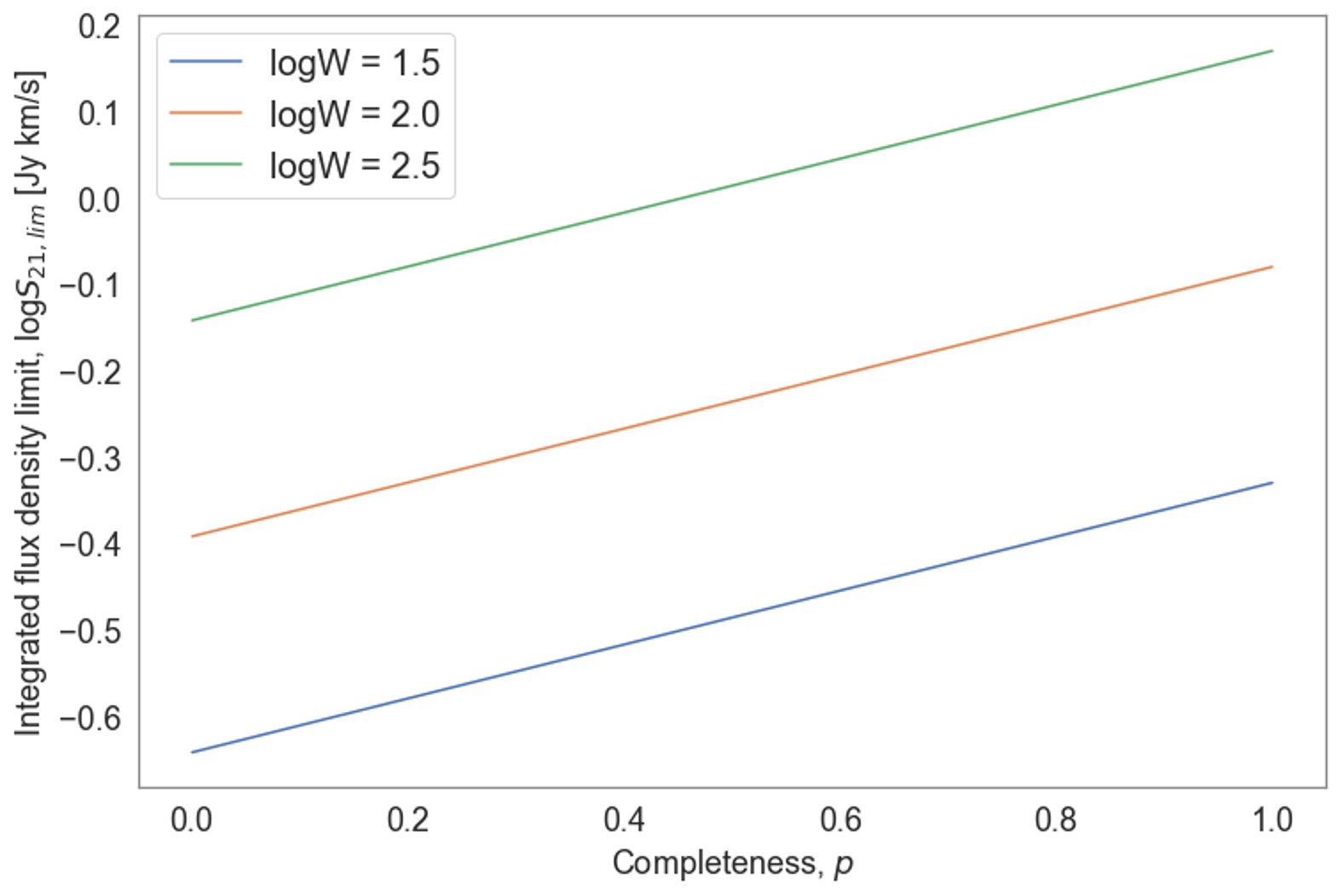
Figure 5: ALFALFA flux density limit as a function of completeness for three choices of velocity width.

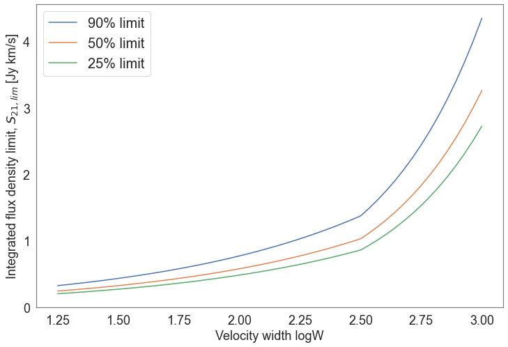
Figure 6: ALFALFA flux density limit as a function of velocity width for 25%, 50%, and 90% completeness.

Rosenberg & Schneider (2002) have shown that adopting a step function based on the 50% completeness limit of a survey produces approximately the same results as adopting the survey’s full completeness function. In Appendix A, we demonstrate that in the case of ALFALFA, using the 50% completeness instead of the full completeness function results in a 4.7% underestimation of the selection function for any galaxy in the sample. We therefore choose to use the full completeness function to derive our selection function.

Eq. 8 gives a general expression for the selection function $S_{n}$. In the ALFALFA survey, $z_{\textrm{min}}\sim 0$ and $z_{\textrm{max}}=0.06$ are the upper and low redshift limits, and $V(z_{\textrm{min}})$ and $V(z_{\textrm{max}})$ are the corresponding comoving volumes. The comoving volume $V_{C}$ is related to the comoving distance $D_{C}$ by

$$V_{C}=\frac{4\pi f_{\textrm{sky}}}{3}D_{C}^{3}$$ (29)

where $f_{\textrm{sky}}$ is the fraction of the whole sky covered by the volume.

This simplifies the selection function to

$$S_{n}=\left(\frac{D_{n}^{\textrm{max}}}{177\,\textrm{Mpc}}\right)^{3}$$ (30)

where $D_{n}^{\textrm{max}}$ is the maximum comoving distance at which galaxy $n$ can be detected in the survey given its flux and linewidth, and $D_{\textrm{max}}=177$ Mpc corresponds to $z_{\textrm{max}}=0.06$ in our assumed cosmology. If $D_{n}^{\textrm{max}}>177$ Mpc, we impose $S_{n}=1$. Now we must derive an expression for $D_{n}^{\textrm{max}}$.

H I mass can be converted to velocity-integrated flux density (in the observed frame) using the standard equation give, e.g., by Meyer et al. (2017)

$$M_{\textrm{HI}}=2.356\times 10^{5}D^{2}_{L}S_{21}(1+z)^{-2}$$ (31)

where $M_{\textrm{HI}}$ is in units of solar masses, $D_{L}$ is the luminosity distance in units of Mpc, and the $S_{21}$ is the velocity integrated flux in units of Jy km s^-1. In terms of co-moving distance, this becomes

$$M_{\textrm{HI}}=2.356\times 10^{5}D^{2}_{C}S_{21}~{}.$$ (32)

For a galaxy with H I mass $M_{\textrm{HI}}$, we have a measured flux $S_{21}$ and an unknown distance $D_{C}$. The flux limit $S_{21,\textrm{lim}}$ corresponds to the maximum possible distance $D_{C}^{\textrm{max}}$ at which this galaxy can be detected,

$$M_{\textrm{HI}}=2.356\times 10^{5}(D^{\textrm{max}}_{C})^{2}S_{21,\textrm{lim}}~{}.$$ (33)

This gives

$$(D_{C}^{\textrm{max}})^{2}S_{21,\textrm{lim}}=D_{C}^{2}S_{21}~{}.$$ (34)

Combined with Eq. 30, we end up with the following expression for the selection function:

$$S_{n}=\begin{cases}1&D_{n}^{\textrm{max}}\geq 177\textrm{Mpc}\\ \frac{D_{C}^{3}S_{21}^{3/2}}{10^{3B/2}(177\,\textrm{Mpc})^{3}}\int_{0}^{1}10^{-3Ap/2}dp.&D_{n}^{\textrm{max}}<177\textrm{Mpc}\end{cases}$$ (35)

where $A$ and $B$ are determined from interpolating between the completeness functions given in Haynes et al. (2011); $A=0.312$ and so the value of the integral is 0.612, while $B$ is a function of $\log{W_{m50}}$.

We see that the selection function for any given galaxy $n$ depends on its distance, flux density, and velocity width. We compute Eq. 35 for the ALFALFA subset of the CF4 dataset, where distance was estimated using the peculiar velocity model of Said et al. (2020). The distribution of selection function values for this dataset is shown in Fig. 7.

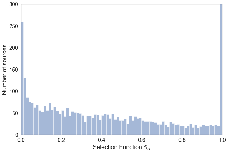
Figure 7: The distribution of the selection function values for the ALFALFA subset of the CF4 dataset. The full height of the last bin is truncated here. There are 1,491 galaxies with $S_{n}=1$.

For the CF4 data, where only 21cm magnitudes are provided, we use the equation given by Kourkchi et al. (2020b) to obtain the integrated 21cm flux in Jy km s^-1

$$\log{S_{21}}=\frac{17.40-m_{21}}{2.5}$$ (36)

where $m_{21}$ is the H I apparent magnitude.

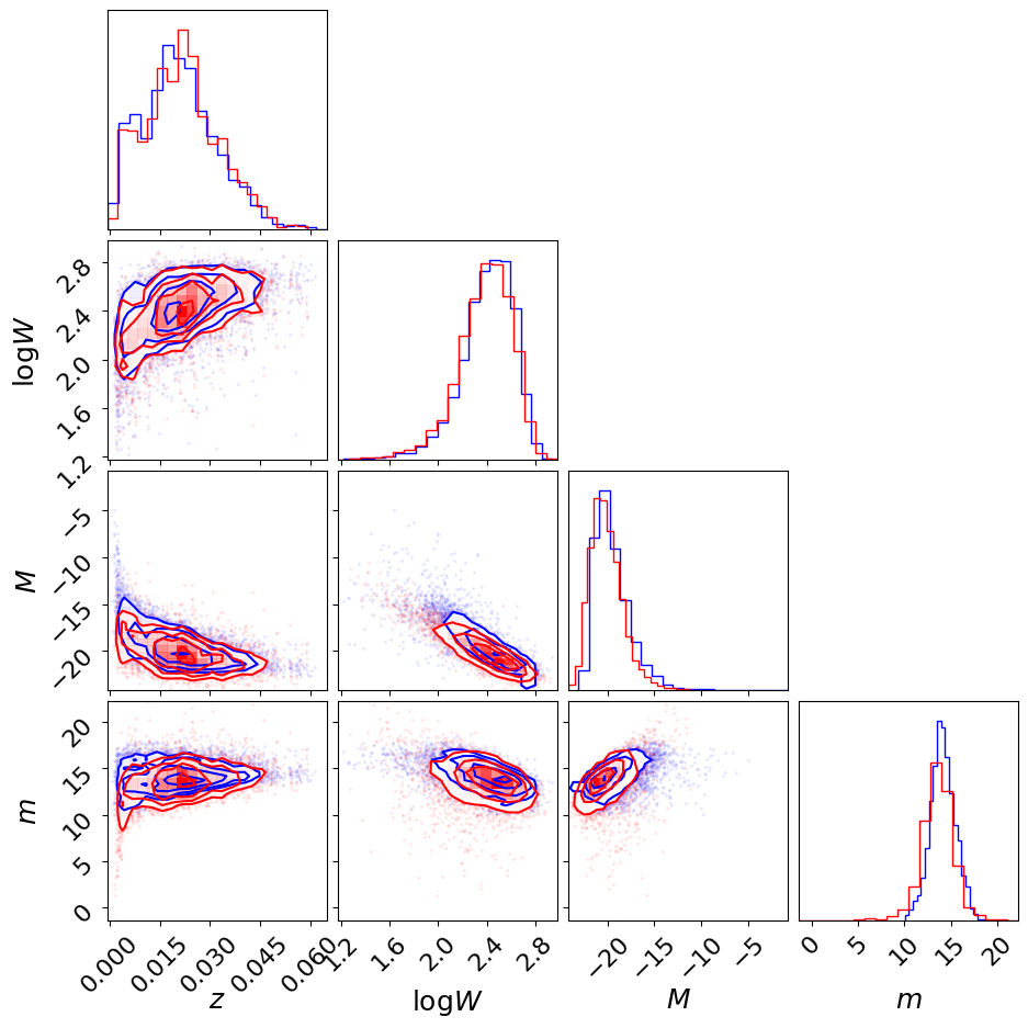
Figure 8: Distributions of the observable quantities (redshift, magnitude, and velocity width) for the mock catalogue (red) compared to the ALFALFA subset of CF4 data (blue).

5.3 Procedure for generating mocks

Given the ingredients described in the previous two sections, we here outline the full procedure used for generating the mock sample.

1. To start, a sample of redshifts is generated by bootstrapping the redshift distribution of the ALFALFA subset of the CF4 survey.

2. For each galaxy redshift, the H I mass corresponding to the low-end flux limit is computed using

   $$M_{\textrm{HI,lim}}=2.356\times 10^{5}D^{2}_{L}S_{21,\textrm{lim}}~{}{\rm M}_{\hbox{$\odot$}},$$ (37)

   where $D_{L}$ is the luminosity distance in Mpc.

3. An H I mass is assigned to each galaxy by sampling from the H I mass function:

   $$\phi(M_{\textrm{HI}})={\rm ln}(10)\phi_{*}\left(\frac{M_{\textrm{HI}}}{M_{*}}\right)^{\alpha+1}{\rm exp}\left(-\frac{M_{\textrm{HI}}}{M_{*}}\right)$$ (38)

   truncated below $M_{\textrm{HI,lim}}$, the H I mass corresponding to the flux limit.

4. For each galaxy, given its H I mass, an observed H I line width at 50% mean flux $W_{m50}$, is sampled from the appropriate conditional velocity width distribution. For this, we assume a Gumbel distribution, with parameters determined by Oman (2021).

5. These steps give us the intrinsic source list. The ALFALFA completeness is then computed for each galaxy in this list, and the galaxy included or excluded based on that probability. This yields the observed source list.

6. Following the processing steps of the Cosmicflows-4 catalogue (Kourkchi et al., 2020b), observed linewidths at 50% average H I flux $W_{m50}$ are corrected for spectral resolution and redshift:

   $$W_{m50}^{c}=\frac{W_{m50}}{1+z}-2\lambda\Delta\nu$$ (39)

   and linewidths are further adjusted to approximate twice the (projected) maximum rotation ($W_{mx}\sim 2V_{\textrm{max}}\sin(i)$) following Courtois et al. (2009):

   $$W_{mx}=W_{m50}^{c}-6\,\textrm{km\,s}^{-1}$$ (40)

7. A random inclination $i$ is chosen from the distribution of observed CF4 inclinations. Each $W_{mx}$ is de-projected for the inclination $i$ to compute a $W_{\textrm{mx}}^{c}$:

   $$W_{\textrm{mx}}^{c}=W_{mx}/\sin i$$ (41)

8. The Tully-Fisher relation is used to compute an absolute magnitude $M$ corresponding to each $W_{\textrm{mx}}^{c}$, and a random error is added from a Gaussian of width given by the intrinsic scatter model.

9. The apparent magnitude is calculated using the absolute magnitude and galaxy redshift.

10. Using the position and redshift of each galaxy, a peculiar velocity is computed from the model in Eq. 27 based on the 2M++ redshift compilation.

Fig. 8 shows the resulting distributions of the mean values for the observable quantities of the mocks. Each distribution is compared to the Cosmicflows-4 dataset we are trying to emulate. The mocks are in good agreement with the Cosmicflows-4 data.

We apply the methodology of Section 4 to our mocks using the input parameters listed in Table 2. The resulting parameter constraints are shown in Fig. 9 and are consistent with the input values.

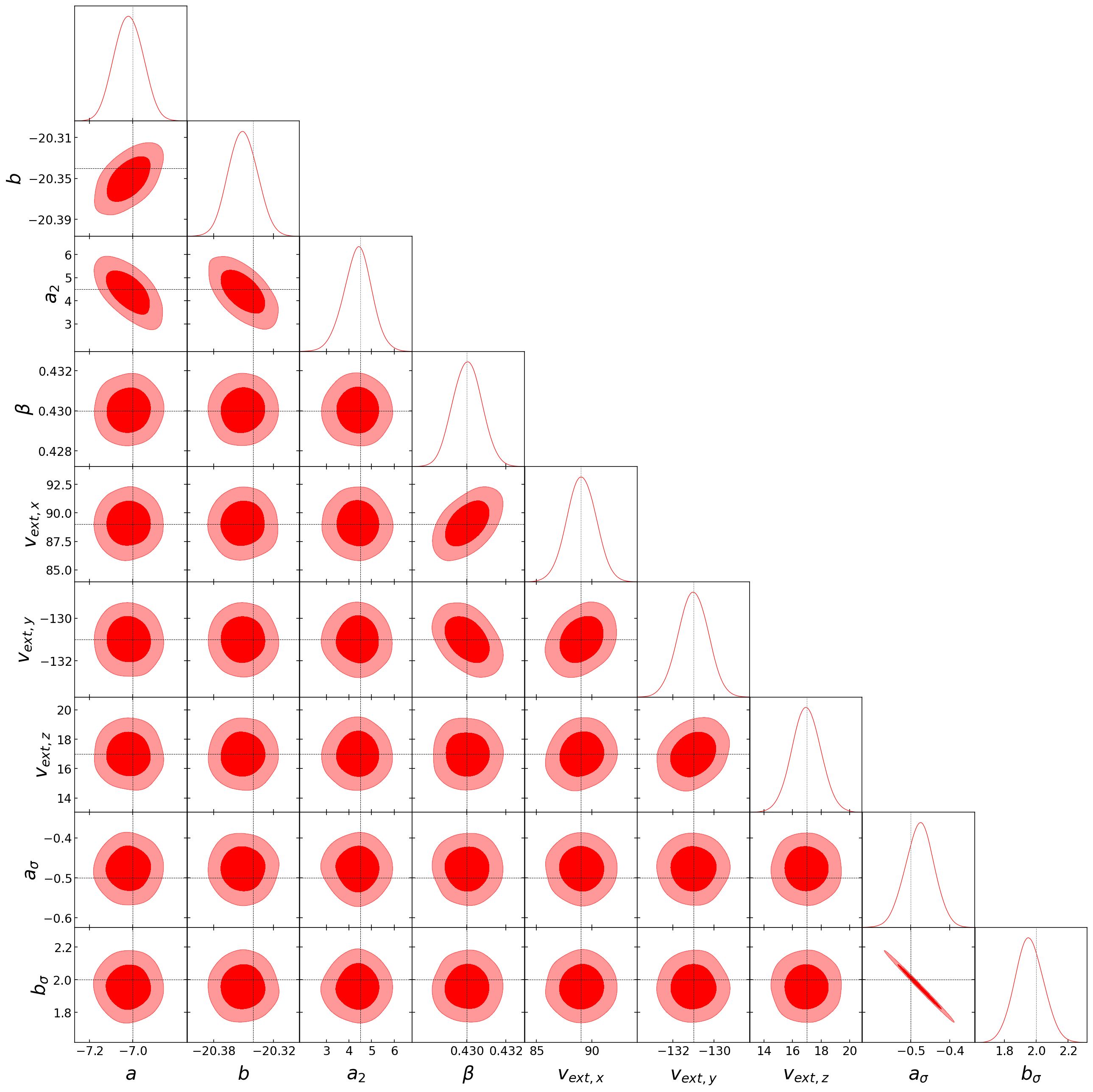
Figure 9: Constraints obtained for the mock CF4 sample, with input values indicated by grey crosshairs; the dark and light colourings show the 68% and 95% confidence regions for the pairwise joint posterior probabilities. The parameters $a$, $b$ and $a_{2}$ represent the slope, intercept and curvature coefficient of the Tully-Fisher relation; $a_{\sigma}$ and $b_{\sigma}$ are the slope and intercept of the Tully-Fisher scatter model. The parameter $\beta$ is the velocity field scaling parameter and ($v_{\textrm{ext},y}$, $v_{\textrm{ext},y}$, $v_{\textrm{ext},z}$) are the bulk flow components; all of these are from the peculiar velocity model.

6 Results

Having tested this work’s methodology on mock data, we proceeded to implement it on the ALFALFA subset of CF4. This section outlines the main results of this analysis.

Table 3: Parameters of the Tully-Fisher relation and peculiar velocity field for the ALFALFA subset of the Cosmicflows-4 sample.

Parameter	Value
Tully-Fisher model
$a$	$-$7.6 $\pm$ 0.1
$b$	$-$20.364 $\pm$ 0.009
$a_{2}$	6.1 $\pm$ 0.6
$a_{\sigma}$	$-$0.69 $\pm$ 0.04
$b_{\sigma}$	2.37 $\pm$ 0.09
Peculiar velocity model
$\beta$	0.40$\pm$0.07
$v_{\textrm{ext},x}$	69$\pm$15 km s-1
$v_{\textrm{ext},y}$	$-$158$\pm$9 km s-1
$v_{\textrm{ext},z}$	14$\pm$7 km s-1

6.1 Measurements of growth rate and Tully-Fisher parameters

Fig. 10 shows the pairwise posterior probability contours for the parameters of the Tully-Fisher model ($a$, $b$, $a_{2}$, $a_{\sigma}$, $b_{\sigma}$) and the peculiar velocity model ($\beta$, $v_{\textrm{ext},x}$, $v_{\textrm{ext},y}$, $v_{\textrm{ext},z}$) obtained using our method applied to the ALFALFA subset of CF4; Table 3 lists the corresponding parameter estimates and uncertainties.

The bulk flow is $\mathbf{V}_{\textrm{ext}}$=(69$\pm$15,$-$158$\pm$9,14$\pm$7) km s^-1 in Supergalactic coordinates. This agrees with previous measurements: Carrick et al. (2015) found $\mathbf{V}_{\textrm{ext}}$=(89$\pm$21,$-$131$\pm$23,17$\pm$26) km s^-1 for the 2M++ volume, Boruah et al. (2021) found $\mathbf{V}_{\textrm{ext}}$=(88$\pm$13,$-$146$\pm$11,0$\pm$9) km s^-1, and Said et al. (2020) found $\mathbf{V}_{\textrm{ext}}$=(94$\pm$10,$-$138$\pm$12,4$\pm$12) km s^-1.

The fitted Tully-Fisher relation parameters for our sample of $7341$ ALFALFA galaxies are $a=-7.6\pm 0.1$, $b=-20.364\pm 0.009$, and $a_{2}=6.1\pm 0.6$, with the break point fixed at $d=\log{W_{\textrm{mx}}^{c}}-2.5=0$. Kourkchi et al. (2020a) calibrated the Tully-Fisher relation using a subsample of $\sim$600 spirals in the CF4 dataset (including non-ALFALFA galaxies). They found that, in the $i$ band, $a=-8.32\pm 0.13$, $b=-20.80\pm 0.10$, and $a_{2}=5.34\pm 0.91$ at a break point of $d=0$. Masters et al. (2006) also derived a linear $i$-band Tully-Fisher relation for a subsample of SFI++ that contained 807 galaxies; their fit was $a=-7.85\pm 10$ and $b=-20.85\pm 0.02$. The differences between these relations are largely due to the very different samples of galaxies used in the calibrations.

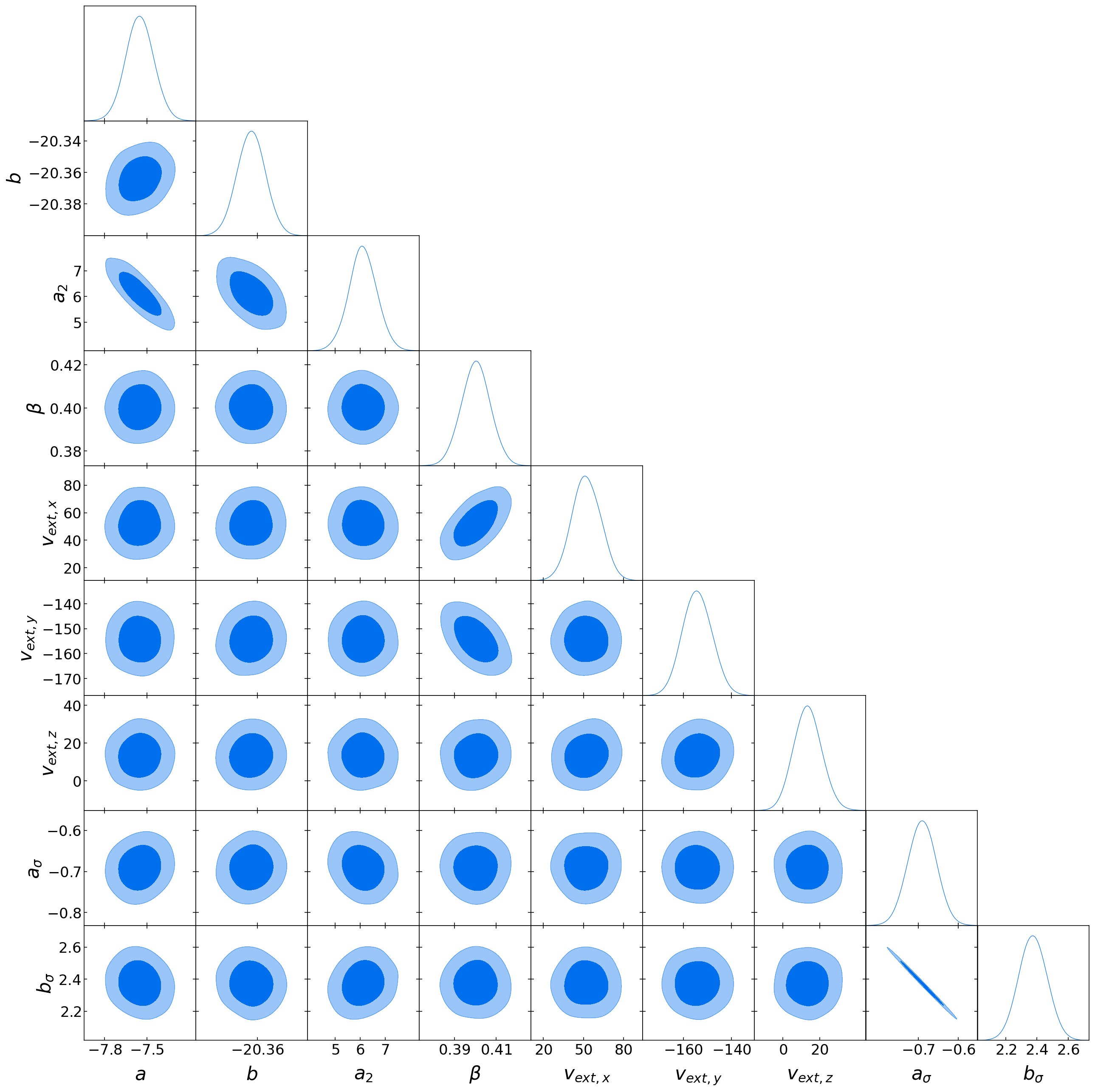
Figure 10: Results of our methodology applied to the ALFALFA subset of CF4 using the 2M++ model for density and peculiar velocity fields. The dark and light colourings show the 68% and 95% confidence regions for the pairwise joint posterior probabilities using the curved Tully-Fisher relation with linear scatter model; the break-point is fixed at $d=0$.

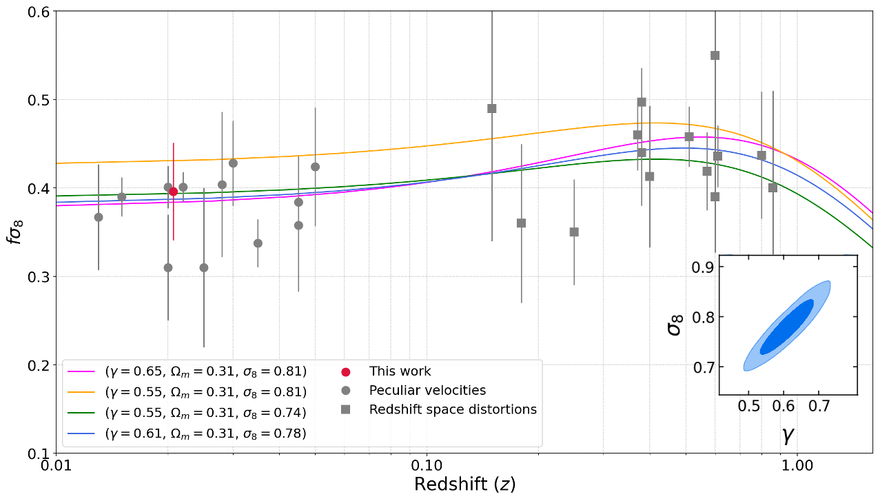
Figure 11: Comparison of $f\sigma_{8}$ constraints from various measurements at different redshifts. Measurements and their sources are listed in Table 4. Models for the evolution of $f\sigma_{8}$ over redshift are shown for four different cosmologies. In orange: Planck parameters (Aghanim et al., 2020) with the standard GR $\gamma=0.55$. In pink: the Aghanim et al. (2020) values for $\Omega_{m}$ and $\sigma_{8}$ are fixed and we find that $\gamma=0.65\pm 0.02$ produces the best fit to measurements. In green: $\sigma_{8}=0.74\pm 0.01$ results in the best fit when $\Omega_{m}$ and $\gamma$ are fixed. In blue: both parameters are free, resulting in $\sigma_{8}=0.78\pm 0.04$ and $\gamma=0.61\pm 0.05$. The pairwise joint probability for these two parameters is also shown in the bottom right.

Having obtained a constraint for the $\beta$ velocity field scaling parameter, we can then also derive a constraint for the growth rate of cosmic structure, $f\sigma_{8}$, using $f\sigma_{8}=\beta\sigma_{8,g}$. The parameter $\sigma_{8,g}$ is the RMS fluctuation in galaxy number in spheres of radius 8 $h^{-1}$ Mpc. This can be calculated using redshift data only. For the 2M++ galaxy redshift compilation, $\sigma_{8,g}=0.99$ (Carrick et al., 2015), which results in a growth rate $f\sigma_{8}=0.40\pm 0.07$. This measurement is consistent with those of other estimates at the same redshift ($z=0.02$): Carrick et al. (2015) measured $f\sigma_{8}=0.401\pm 0.024$, Boruah et al. (2021) measured $f\sigma_{8}=0.401\pm 0.017$, and Davis et al. (2011) measured $f\sigma_{8}=0.31\pm 0.06$.

6.2 Comparison of growth rate measurements

Table 4: Comparison of $f\sigma_{8}$ constraints from various measurements at different effective redshifts $z_{\rm eff}$.

$z_{\rm eff}$	$f\sigma_{8}$	Reference
0.013	0.367$\pm$0.06	Lilow & Nusser (2021)
0.015	0.39$\pm$0.022	Stahl et al. (2021)
0.02	0.40$\pm$0.07	This work
0.02	0.31$\pm$0.06	Davis et al. (2011)
0.02	0.401$\pm$0.024	Carrick et al. (2015)
0.022	0.401$\pm$0.017	Boruah et al. (2021)
0.025	0.31$\pm$0.09	Branchini et al. (2012)
0.028	0.404$\pm$0.082	Qin et al. (2019)
0.03	0.428$\pm$0.048	Huterer et al. (2017)
0.035	0.338$\pm$0.027	Said et al. (2020)
0.045	0.384$\pm$0.052	Adams & Blake (2020)
0.045	0.358$\pm$0.075	Turner et al. (2022)
0.05	0.424$\pm$0.067	Adams & Blake (2017)
0.067	0.423$\pm$0.055	Beutler et al. (2012)
0.15	0.49$\pm$0.15	Howlett et al. (2016)
0.18	0.36$\pm$0.09	Blake et al. (2013)
0.25	0.35$\pm$0.06	Samushia et al. (2012)
0.37	0.46$\pm$0.04	Samushia et al. (2012)
0.38	0.497$\pm$0.039	Alam et al. (2017)
0.4	0.413$\pm$0.08	Blake et al. (2012)
0.51	0.458$\pm$0.035	Alam et al. (2017)
0.57	0.419$\pm$0.044	Beutler et al. (2014)
0.6	0.55$\pm$0.12	Pezzotta et al. (2017)
0.61	0.436$\pm$0.034	Alam et al. (2017)
0.8	0.437$\pm$0.072	Blake et al. (2012)
0.86	0.4$\pm$0.11	Pezzotta et al. (2017)

Table 4 and Fig. 11 show that our measurement of $f\sigma_{8}$ is consistent with those of other peculiar velocity analyses (which are exclusively at low redshifts) and with measurements obtained from redshift space distortions at higher redshifts (within the $\Lambda$CDM framework).

Fig. 11 also shows a model prediction for the evolution of the growth rate under GR (the orange curve); for this model, $\Lambda$CDM is used with Planck parameters (Aghanim et al., 2020). Our measurement is consistent with this model. However, all peculiar velocity results lie below this line; some are more than 1$\sigma$ below (Stahl et al., 2021; Davis et al., 2011; Boruah et al., 2021; Branchini et al., 2012; Said et al., 2020; Turner et al., 2022); while theSaid et al. (2020) measurement is more than 3$\sigma$ below. We can improve the agreement between measurements and model by allowing the cosmological parameters $\gamma$, $\Omega_{m}$, and $\sigma_{8}$ to vary. First, we fit with $\gamma$ as a free parameter while fixing $\Omega_{m}$ and $\sigma_{8}$ to the Aghanim et al. (2020) values, which gives $\gamma=0.65\pm 0.02$ as the best fit (pink curve). This result favours Dvali-Gabadadze-Porrati (DGP) gravity (Dvali et al., 2000), which takes on $\gamma=11/16$ (Linder & Cahn, 2007). This is in contrast to General Relativity, for which $\gamma=6/11$ (Wang & Steinhardt, 1998; Linder, 2005). Second, we fit $\sigma_{8}$ while setting $\gamma=0.55$ and $\Omega_{m}=0.31$, and find that a lower fluctuation amplitude of $\sigma_{8}=0.74\pm 0.01$ is favoured (green curve). Lastly, we allow both $\gamma$ and $\sigma_{8}$ to be free and find $\sigma_{8}=0.78\pm 0.04$ and $\gamma=0.61\pm 0.05$; this fit is shown by the blue curve and the inset shows the pairwise joint posterior probability distribution. We note that this is only a naive analysis; it assumes that measurements are independent when in fact they are not. A rigourous analysis would have to take into account the correlated data and would likely produce less stringent constraints as a result.

7 Forecasts for WALLABY

The upcoming Wide-field ASKAP L-band Legacy All-sky Blind surveY (WALLABY) (Koribalski et al., 2020; Courtois et al., 2022) will detect the 21cm linewidth for around 200,000 galaxies at low redshifts ($z<0.1$ and a median redshift $z\sim 0.05$) over 5 years. For about 40% of these galaxies, the signal-to-noise ratio and inclination will be sufficient to reliably determine redshift-independent distances via the Tully-Fisher relation. By 2027, WALLABY is expected to have measured redshift-independent distances with 20% precision for about 100,000 late-type galaxies over half of the sky. The WALLABY sample will provide an independent probe of peculiar velocities within a volume similar to the 6dFGS survey.

A mock catalogue of an ideal WALLABY survey was developed by Koribalski et al. (2020), using the SHARK model for galaxy evolution (Lagos et al., 2018) and the SURFS simulations of cosmic structure (Elahi et al., 2018). Two simulation boxes were used: MICRO-SURFS and MEDI-SURFS. MEDI covers a volume of $210^{3}\,h^{-1}$ Mpc; MICRO covers the nearby Universe with a volume of only $40^{3}\,h^{-1}$ Mpc, but at a much higher resolution.

For each galaxy in the WALLABY mock catalogue, realistic H I line profiles were simulated. This simulated H I data, along with simulated galaxy redshifts, magnitudes, inclinations, and spatial distributions were used, in combination with peculiar velocities from the reconstructed 2M++ velocity field, to provide a realistic mock of the WALLABY Tully-Fisher dataset. The curved Tully-Fisher model described in Section 2 was again applied, with all 6 parameters left free: $a$, $b$, $a_{2}$, $d$, $a_{\sigma}$, and $b_{\sigma}$.

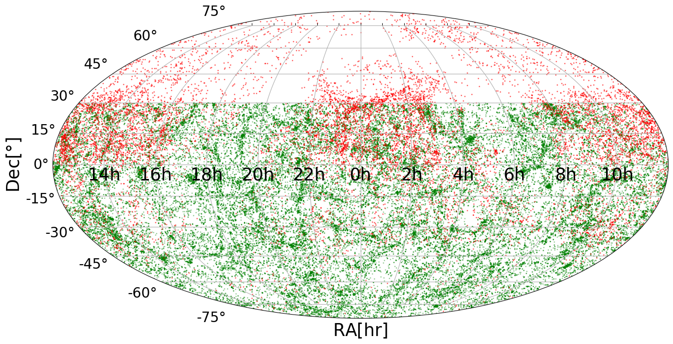
Figure 12: Sky coverage of the full CF4 data (red) and the WALLABY Tully-Fisher reference simulation for galaxies within $z<0.1$ (green).

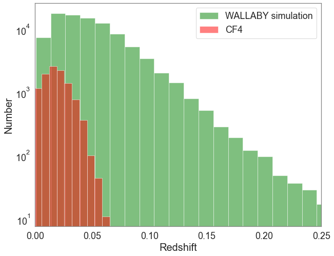
Figure 13: Redshift distributions of the full CF4 sample and the WALLABY Tully-Fisher reference simulation.

While there are over 400,000 galaxies in the full simulation, we reduced this to a more realistic number, given the actual time allocated to the survey and the fact that not all measurements will be suitable for a Tully-Fisher analysis. The main requirements are a sufficiently high signal-to-noise H I measurement (all galaxies in the simulation already pass this test) and inclinations greater than 45$\degree$. An analysis of the WALLABY Pilot Survey (Courtois et al., 2022) provides an estimate that suggests approximately 86,000 distances could be derived at $z<0.1$. Selecting only galaxies with inclinations greater than 45$\degree$, the full WALLABY MEDI simulation was sub-sampled so that the number of galaxies at $z<0.1$ approximately matches this estimate; this resulted in a sample of 89,212 galaxies at $z<0.1$ and 92,828 galaxies over the full redshift range. Fig. 12 shows the sky coverage of the full CF4 data compared to this trimmed-down WALLABY Tully-Fisher reference simulation, while Fig. 13 shows a comparison of the redshift distributions.

We have applied our methodology to this WALLABY Tully-Fisher reference simulation to generate mocks. The breakpoint of the Tully-Fisher relation, $d$, is left as a free parameter in this instance. Fig. 14 and Fig. 16 show the pairwise posterior probability distributions of Tully-Fisher fitting parameters and cosmological parameters for the MICRO and MEDI simulations, while Fig. 15 and Fig. 17 show the resulting Tully-Fisher models fit to the MICRO and MEDI simulations. Table 5 lists the estimated parameter values and uncertainties from the WALLABY Tully-Fisher reference simulation.

Fig. 18 compares the constraints on cosmological parameters obtained from the CF4 analysis ($n$=4622) and the WALLABY Tully-Fisher reference simulation for $z<0.1$ ($n$=89,212). This comparison suggests that WALLABY will yield up to a factor of $~{}4$ improvement on the cosmological constraints obtained from the ALFALFA and Cosmicflows-4 data. To estimate how these more stringent constraints will affect the cosmological parameters $\gamma$ and $\sigma_{8}$, we repeated the fitting performed in Section 6.2 using a WALLABY error bar for the CF4 measurement. We used all redshift space distortion measurements and omitted peculiar velocity measurements aside from our own to isolate the effect of the single improved PV constraint. With the CF4 error, we found $\gamma=0.689\pm 0.053$ and $\sigma_{8}=0.762\pm 0.017$. This became $\gamma=0.639\pm 0.026$ and $\sigma_{8}=0.756\pm 0.014$ when using a WALLABY-like error. The uncertainty in $\gamma$ thereby reduced by 52% and the uncertainty in $\sigma_{8}$ reduced by 20%.

8 Conclusion

In this paper, we present measurements of the velocity field scaling parameter $\beta$ using Tully-Fisher peculiar velocity data from Cosmicflows-4, and derive a constraint on the growth rate of cosmological structure $f\sigma_{8}$. These results are obtained from a Bayesian forward-modelling approach that has not previously been applied to Tully-Fisher peculiar velocities, in which cosmological parameters and Tully-Fisher parameters are fit simultaneously. The conventional linear model for the Tully-Fisher relation is modified to account for the observed curvature at the bright end of the relation and for the varying scatter along the relation. The full model for the Tully-Fisher relation and the peculiar velocity field involves a total of ten parameters: six Tully-Fisher parameters (two for the linear relation, one for the curvature at the bright end, one for the curvature breakpoint, and two for the linear increase in errors to lower velocity widths) and four cosmological parameters (one the scaling parameter $\beta$ for the peculiar velocities based on the density field within the volume and three the components of the bulk motion approximating the effect of the density field outside the volume).

This methodology is tested on mock data in Section 5, confirming that the analysis is able to accurately recover the model parameters of the simulated data. In Section 6, we apply this methodology to Cosmicflows-4 peculiar velocities from the ALFALFA sample, resulting in the parameters for a Tully-Fisher relation with curvature and new constraints for the velocity field scaling parameter ($\beta=0.40\pm 0.07$), the residual bulk flow ($\mathbf{V}_{\textrm{ext}}$ = (9$\pm$15,$-$158$\pm$9,14$\pm$7) km s^-1 in Supergalactic coordinates), and the growth rate $f\sigma_{8}=0.40\pm 0.07$. The growth rate measurement is consistent with other estimates at similar redshifts ($z=0.02$).

The methodology developed for this analysis can also be applied to forthcoming Tully-Fisher peculiar velocity surveys such as WALLABY, which will provide a bounty of new data. In Section 7, existing WALLABY simulations were analysed using this methodology, and it was shown that WALLABY data is well described by the 6-parameter Tully-Fisher model developed in this work. In the best-case scenario, we have found that WALLABY could provide up to a factor $\sim$4.5 improvement on constraints for the cosmological parameters $\beta$ and $\mathbf{V}_{\textrm{ext}}$. As a result, a far more precise measurement of $f\sigma_{8}$ will be obtained at low redshift. This will provide a valuable new data-point in fitting the evolution of the growth rate to cosmological models, as demonstrated in Section 6.2, and will move us closer towards the ultimate goal of understanding the nature of gravity and the growth of cosmic structure.

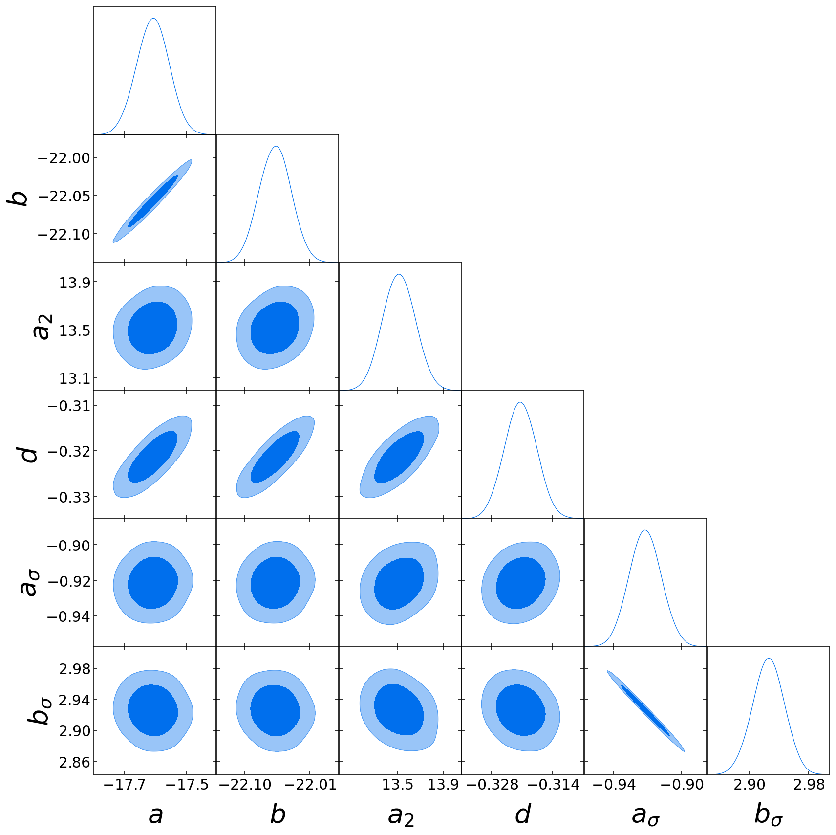
Figure 14: Tully-Fisher parameter constraints obtained from the methodology presented here applied to the MICRO WALLABY reference simulation.

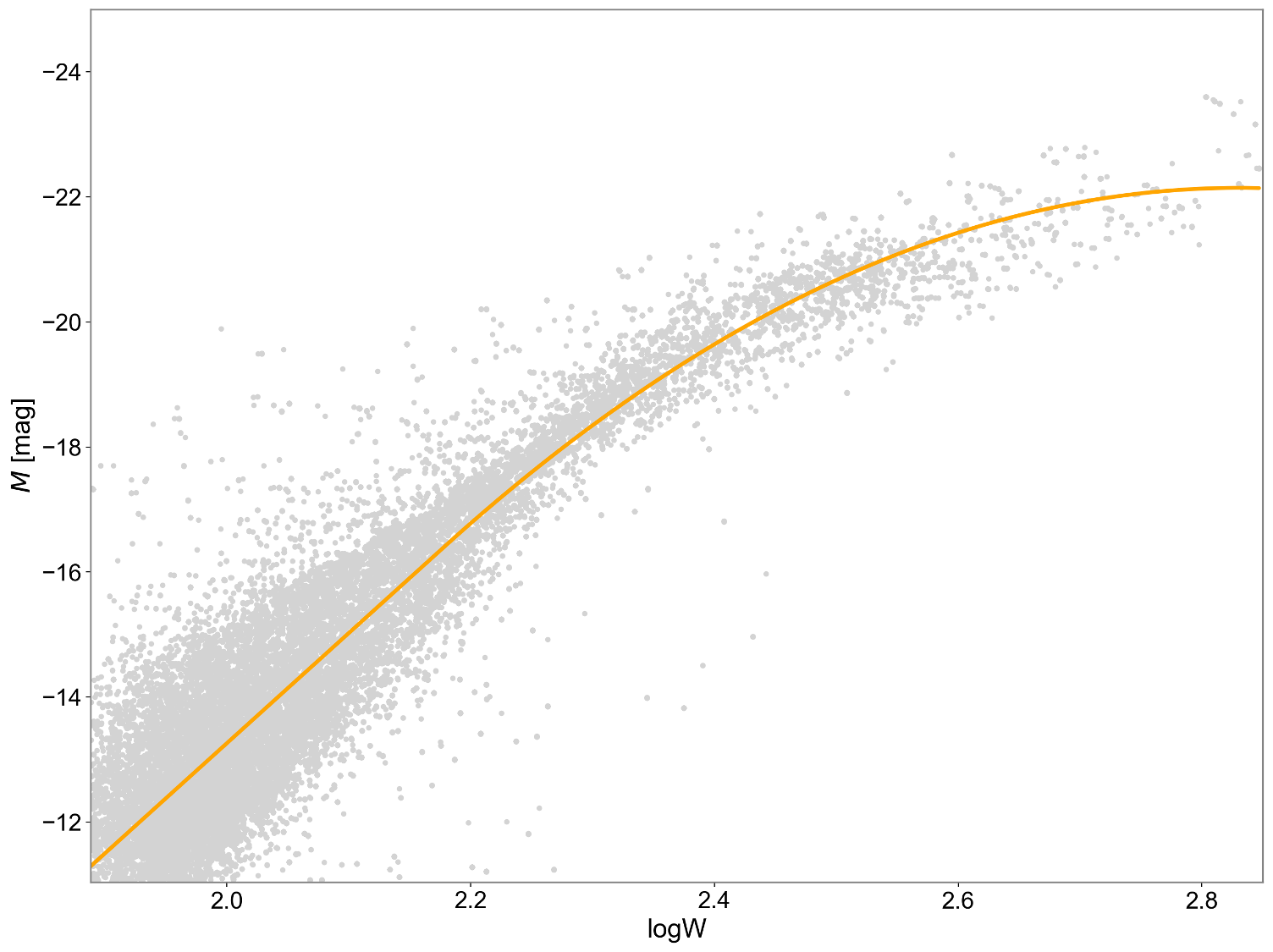
Figure 15: The Tully-Fisher relation of the MICRO WALLABY reference simulation, showing the curved Tully-Fisher model with best-fit parameters from Fig. 14.

Figure 16: Tully-Fisher parameter constraints obtained from the methodology presented in this work applied to the MEDI WALLABY reference simulation.

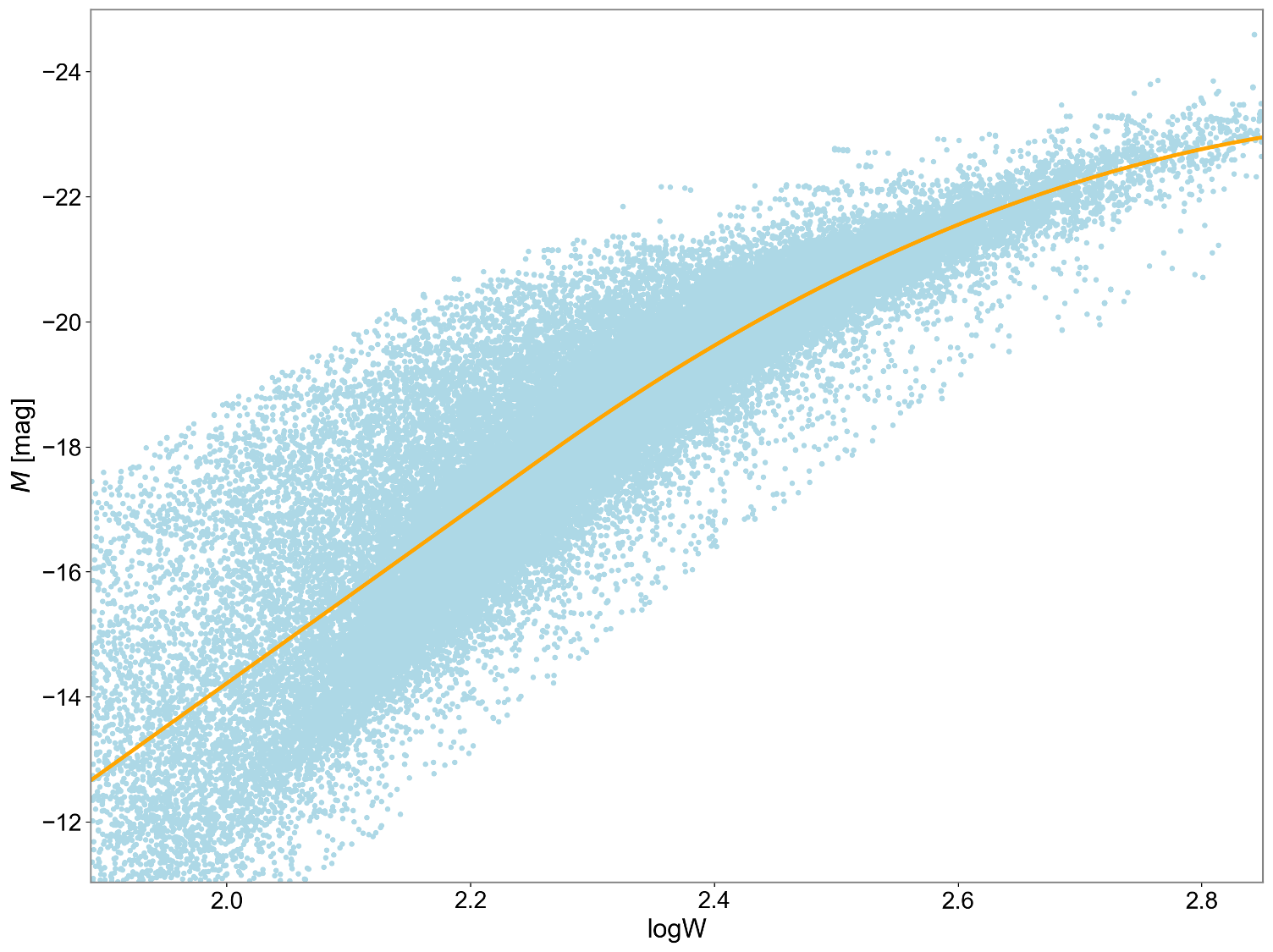
Figure 17: The Tully-Fisher relation for the MEDI WALLABY reference simulation, showing the curved Tully-Fisher model with best-fit parameters from Fig. 16; estimated values and uncertainties are listed in Table 5.

Table 5: Parameter constraints obtained from the WALLABY Tully-Fisher reference simulation with $z<0.1$.

Parameter	Value
Tully-Fisher model
$a$	$-$13.91 $\pm$ 0.05
$b$	$-$21.18 $\pm$ 0.01
$d$	$-$0.234 $\pm$ 0.004
$a_{2}$	9.06 $\pm$ 0.08
$a_{\sigma}$	$-$1.29 $\pm$ 0.06
$b_{\sigma}$	3.82 $\pm$ 0.01
Peculiar velocity model
$\beta$	0.430 $\pm$ 0.001
$v_{\textrm{ext},x}$	89.1 $\pm$ 0.2 km s-1
$v_{\textrm{ext},y}$	$-$130.9 $\pm$ 0.2 km s-1
$v_{\textrm{ext},z}$	17.2 $\pm$ 0.2 km s-1

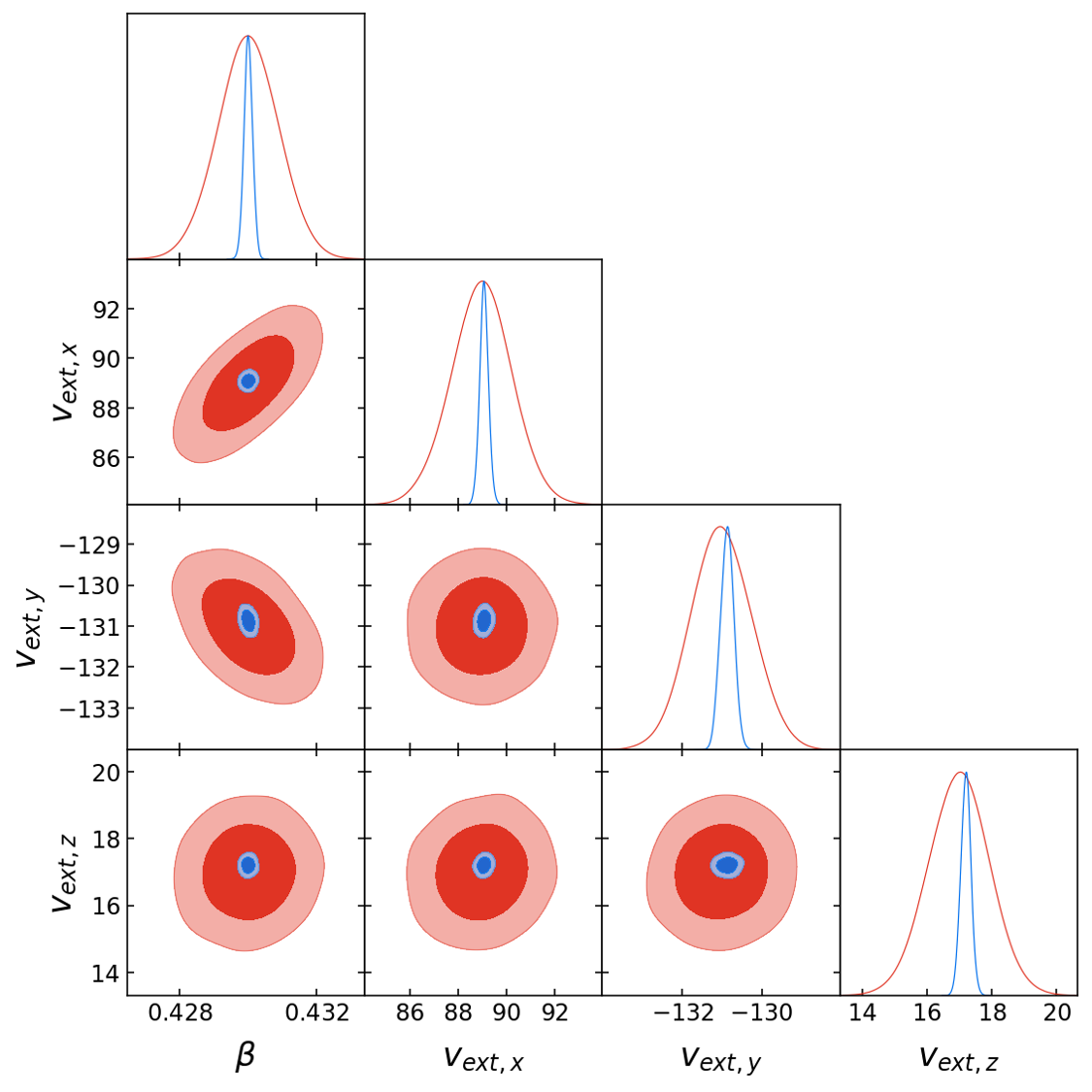
Figure 18: Comparison of cosmological parameter constraints from this analysis using Cosmicflows-4 mocks (red contours) and forecast constraints from the WALLABY reference simulation (blue contours). Estimated values and uncertainties are listed in Table 5.

Data Availability

This work uses previously published data as referenced and described in text. Details of the analysis and code can be made available upon reasonable request to the corresponding author.

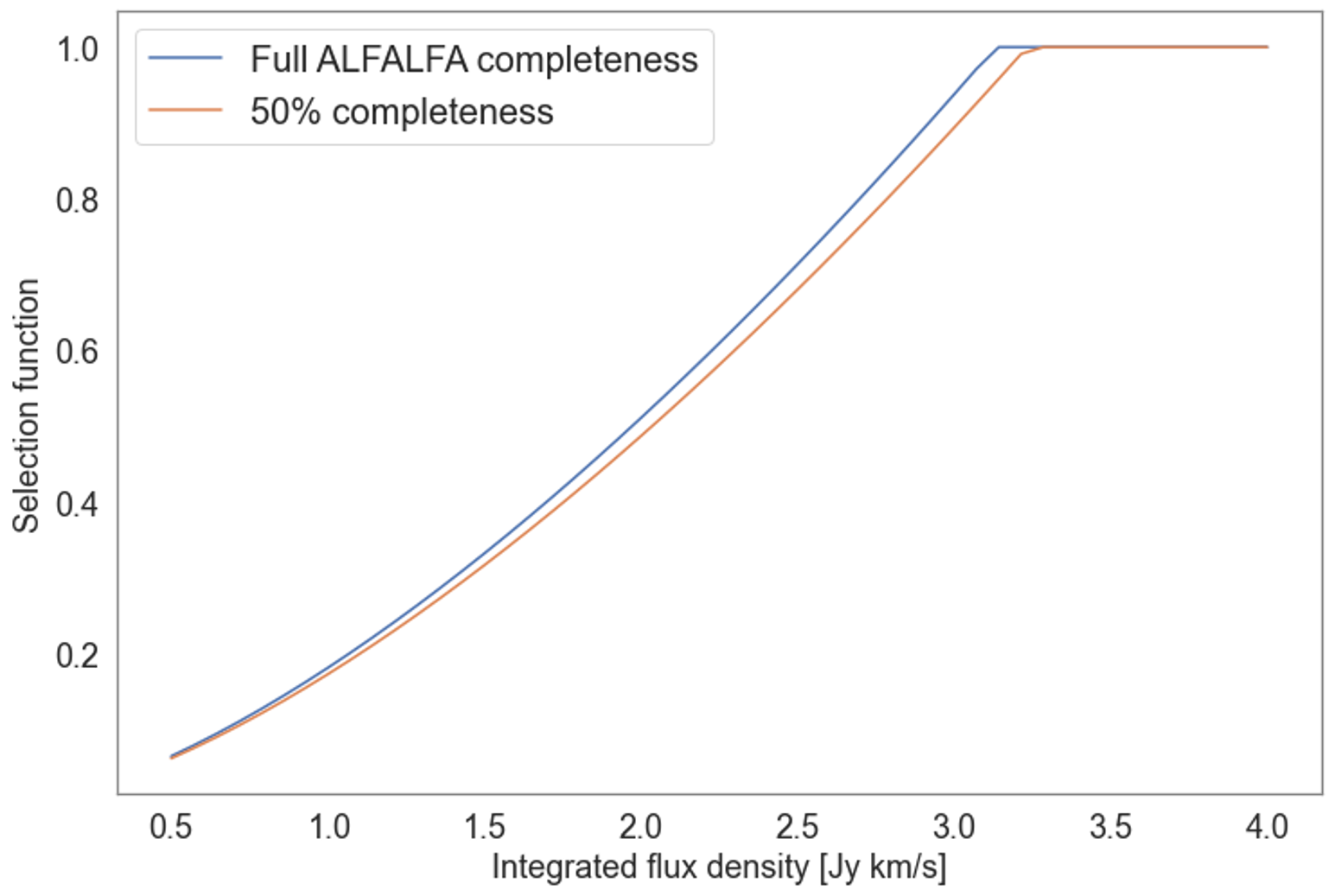
Figure 19: ALFALFA selection function, comparing use of a step function at the 50% completeness limit to integrating over the full completeness function at a co-moving distance $D_{C}=100$ Mpc and a linewidth $\log{W_{m50}}=2.5$.

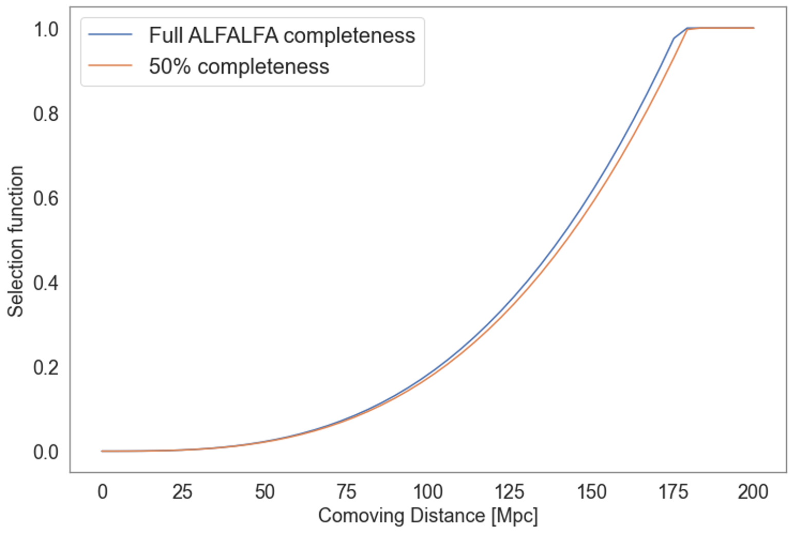
Figure 20: ALFALFA selection function, comparing use of a step function at the 50% completeness limit to integrating over the full completeness function at a linewidth $\log{W_{m50}}$=2.5 and an integrated flux density $S_{21}$=1 Jy km s^-1.

Appendix A Completeness function

Fig. 19 and Fig. 20 show the ALFALFA selection function computed using either the full completeness limit (Eq. 35) or a cutoff at the 50% limit (i.e. substituting $S_{21,\textrm{lim}}(p)=S_{21,\textrm{lim}}(p=0.5)$ instead of integrating over the full completeness function $S_{21,\textrm{lim}}(p)$). The fractional difference between the two selection functions is a constant, $-$4.7%, related to the quantities $A$ and $B$.

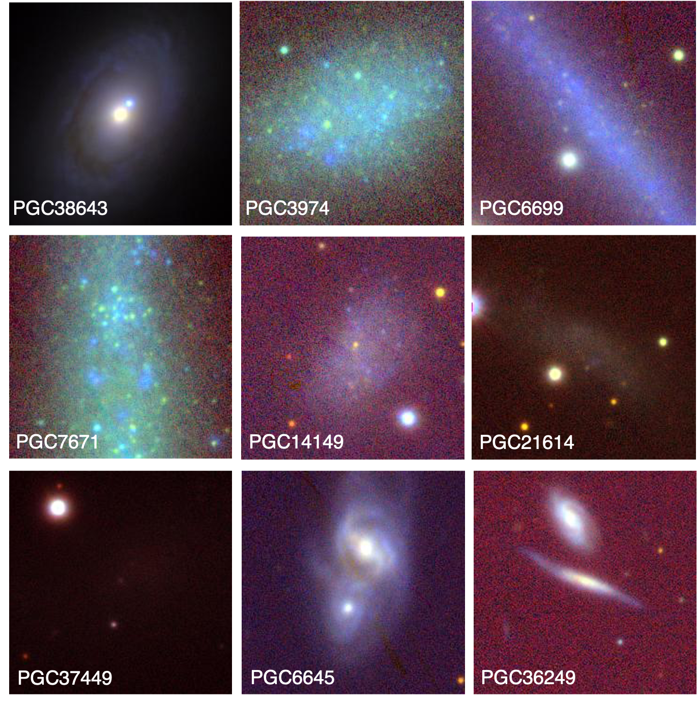
Figure 21: Uniformly scaled images of outlier galaxies (combined $y$, $i$ and $g$ filters) downloaded from the Pan-STARRS image cutout server accessed at https://ps1images.stsci.edu/cgi-bin/ps1cutouts.

Appendix B Outliers

In the ALFALFA subset of the CF4 dataset there were about 150 or so galaxies that were more than 3$\sigma$ away from the best-fit Tully-Fisher relation. We visually inspected the Pan-STARRS images at each source’s coordinates and identified several categories of issues:

• Galaxies that appear clearly inconsistent with their assigned inclination. Galaxies in the CF4 samples are nominally limited to those with inclinations greater than 45 degrees, so anything appearing to be completely face-on is excluded. (Note that inclinations of the CF4 sample were assigned by eye.)

• Galaxies contaminated by very bright nearby sources.

• Galaxy mergers.

• Very large galaxies with lengths exceeding the field of view.

• Images containing only faint blurs or resolved dwarf galaxies.

• Images containing no evident galaxies.

Cases suffering from these obvious issues were excluded from the analysis; this resulted in the removal of 115 outliers (out of $\sim$150). Fig. 21 shows examples of the galaxies that were removed.

References

- Adams & Blake (2017) Adams C., Blake C., 2017, MNRAS , 471, 839
- Adams & Blake (2020) Adams C., Blake C., 2020, MNRAS , 494, 3275
- Aghanim et al. (2020) Aghanim N., et al., 2020, A&A, 641, A6
- Alam et al. (2017) Alam S., et al., 2017, MNRAS , 470, 2617
- Beutler et al. (2012) Beutler F., et al., 2012, MNRAS , 423, 3430
- Beutler et al. (2014) Beutler F., et al., 2014, MNRAS , 443, 1065
- Blake et al. (2012) Blake C., et al., 2012, MNRAS , 425, 405
- Blake et al. (2013) Blake C., et al., 2013, MNRAS , 436, 3089
- Boruah et al. (2021) Boruah S. S., Hudson M. J., Lavaux G., 2021, MNRAS , 507, 2697
- Branchini et al. (2012) Branchini E., Davis M., Nusser A., 2012, MNRAS , 424, 472
- Carr et al. (2022) Carr A., Davis T. M., Scolnic D., Said K., Brout D., Peterson E. R., Kessler R., 2022, PASA , 39, e046
- Carrick et al. (2015) Carrick J., Turnbull S. J., Lavaux G., Hudson M. J., 2015, MNRAS , 450, 317–332
- Colless et al. (2001) Colless M., Saglia R. P., Burstein D., Davies R. L., McMahan R. K., Wegner G., 2001, MNRAS , 321, 277
- Courtois et al. (2009) Courtois H. M., Tully R. B., Fisher J. R., Bonhomme N., Zavodny M., Barnes A., 2009, AJ, 138, 1938–1956
- Courtois et al. (2022) Courtois H. M., et al., 2022, MNRAS , 519, 4589
- Davis et al. (2011) Davis M., Nusser A., Masters K. L., Springob C., Huchra J. P., Lemson G., 2011, MNRAS , 413, 2906
- Dvali et al. (2000) Dvali G., Gabadadze G., Porrati M., 2000, Phys. Lett. B, 485, 208
- Elahi et al. (2018) Elahi P. J., Welker C., Power C., del P Lagos C., Robotham A. S. G., Cañ as R., Poulton R., 2018, MNRAS , 475, 5338
- Foreman-Mackey et al. (2013) Foreman-Mackey D., Hogg D. W., Lang D., Goodman J., 2013, PASP, 125, 306
- Haynes et al. (2011) Haynes M. P., et al., 2011, AJ, 142, 170
- Haynes et al. (2018) Haynes M. P., et al., 2018, ApJ , 861, 49
- Howlett et al. (2016) Howlett C., Staveley-Smith L., Blake C., 2016, MNRAS , 464, 2517–2544
- Howlett et al. (2022) Howlett C., Said K., Lucey J. R., Colless M., Qin F., Lai Y., Tully R. B., Davis T. M., 2022, MNRAS , 515, 953
- Hunter (2007) Hunter J. D., 2007, Comput. Sci. Eng., 9, 90
- Huterer et al. (2017) Huterer D., Shafer D. L., Scolnic D. M., Schmidt F., 2017, J. Cosmology Astropart. Phys., 2017, 015
- Koribalski et al. (2020) Koribalski B. S., et al., 2020, ApSS , 365
- Kourkchi et al. (2020a) Kourkchi E., Tully R. B., Anand G. S., Courtois H. M., Dupuy A., Neill J. D., Rizzi L., Seibert M., 2020a, ApJ , 896, 3
- Kourkchi et al. (2020b) Kourkchi E., et al., 2020b, ApJ , 902, 145
- Lagos et al. (2018) Lagos C., Tobar R. J., Robotham A. S. G., Obreschkow D., Mitchell P. D., Power C., Elahi P. J., 2018, MNRAS , 481, 3573
- Lewis (2019) Lewis A., 2019, GetDist: a Python package for analysing Monte Carlo samples
- Lilow & Nusser (2021) Lilow R., Nusser A., 2021, MNRAS , 507, 1557
- Linder (2005) Linder E. V., 2005, Phys. Rev. D, 72
- Linder & Cahn (2007) Linder E. V., Cahn R. N., 2007, Astropart. Phys., 28, 481
- Masters et al. (2006) Masters K. L., Springob C. M., Haynes M. P., Giovanelli R., 2006, ApJ , 653, 861
- Meyer et al. (2017) Meyer M., Robotham A., Obreschkow D., Westmeier T., Duffy A. R., Staveley-Smith L., 2017, PASA , 34
- Oman (2021) Oman K. A., 2021, MNRAS , 509, 3268
- Peterson et al. (2022) Peterson E. R., et al., 2022, ApJ , 938, 112
- Pezzotta et al. (2017) Pezzotta A., et al., 2017, A&A, 604, A33
- Qin et al. (2019) Qin F., Howlett C., Staveley-Smith L., 2019, MNRAS , 487, 5235
- Robitaille et al. (2013) Robitaille T. P., et al., 2013, A&A, 558, A33