Robust propagation-based phase retrieval for CT in proximity to highly attenuating objects

Abstract

X-ray imaging is a fast, precise and non-invasive method of imaging which, combined with computed tomography, provides detailed 3D rendering of samples. Incorporating propagation-based phase contrast can vastly improve data quality for weakly attenuating samples via material-specific phase retrieval filters, allowing radiation exposure to be reduced. However, applying phase retrieval to multi-material phantoms complicates analysis by requiring a choice of which material boundary to tune the phase retrieval. Filtering for the boundary with strongest phase contrast increases noise suppression, but with the detriment of over-blurring other interfaces, potentially obscuring small or neighbouring features and removing quantitative sample information. Additionally, regions bounded by more than one material type inherently cannot be conventionally filtered to reconstruct the whole boundary. As remedy, we present a computationally-efficient, non-iterative nor AI-mediated method for applying strong phase retrieval, whilst preserving sharp boundaries for all materials within the sample. This technique was tested on phase contrast images of a rabbit kitten brain encased by the surrounding dense skull. Using $24\text{\,}\mathrm{k}\mathrm{e}\mathrm{V}$ synchrotron radiation with a $5\text{\,}\mathrm{m}$ propagation distance, our technique provided a 6.9-fold improvement in the signal-to-noise ratio (SNR) of brain tissue compared to the standard phase retrieval procedure, without over-smoothing the images. Simultaneous quantification of edge resolution and SNR gain was performed with an aluminium-water phantom imaged using a microfocus X-ray tube at mean energy $19.58\text{\,}\mathrm{k}\mathrm{e}\mathrm{V}$ and $0.576\text{\,}\mathrm{m}$ effective propagation distance. Our method provided a 4.2-fold SNR boost whilst preserving the boundary resolution at $54\pm 1\text{\,}\mathrm{\SIUnitSymbolMicro m}$, compared to $108\pm 2\text{\,}\mathrm{\SIUnitSymbolMicro m}$ in conventional phase retrieval.

Keywords X-ray Imaging, Phase-retreival, High contrast, Multi-material

1 Introduction

X-ray imaging can provide high-resolution, three-dimensional (3D) visualisation of the internal structure of an object when combined with computed tomography (CT). However, capturing high-resolution CT images with high signal-to-noise (SNR) ratio using standard x-ray systems requires a non-negligible radiation dose, potentially harming samples that are sensitive to ionising radiation. Clinical imaging systems limit radiation exposure by using highly efficient X-ray detectors, with relatively low resolution being the typical trade-off. Iterative reconstruction algorithms may also be used to help balance this compromise[1].

High-resolution CT scans of biological tissues can be achieved with low radiation dose by using phase contrast x-ray imaging [2][3]. Phase contrast imaging uses specific setups to transform phase effects, introduced by the sample, into intensity variations capable of being recorded by detectors, and hence provides more information than from absorption contrast alone. While several x-ray phase contrast techniques exist, we focus here on propagation-based imaging (PBI), taking advantage of the simplicity in optical design that only requires a sufficiently coherent x-ray wavefield at the sample position and some propagation distance between the sample and detector. Phase contrast arises from interference between x-rays that have incurred different phase shifts as they pass through an object. This results in intensity fringes appearing along material boundaries at the detector plane, effectively acting as a sharpening filter [4]. This is particularly valuable for those boundaries between low-Z materials, which are weakly-attenuating and hence create only weak attenuation contrast. To restore the sample structure requires the application of a phase-retrieval algorithm. For objects comprised of a single monomorphous material, the algorithm of Paganin et. al [5] accomplishes this using a low-pass filter specifically tuned to suppress phase contrast fringes at the boundaries of the object, whilst also providing SNR amplification by suppressing high-frequency noise. The algorithm can be represented by

$$I(x,y) =\mathcal{F}^{-1}\left\{\frac{\mathcal{F}[I_{d}(x,y)/I_{0}]}{1+\frac{\delta\Delta}{\mu}\textbf{k}_{\perp}^{2}}\right\},$$ (1)

where $\mathcal{F}$ and $\mathcal{F}^{-1}$ are the forward and reverse Fourier transform operators, $I_{d}(x,y)$ is the image measured at the detector plane, $I_{0}$ is the spatially variable incident intensity, $\Delta$ is the propagation distance from object to detector, and $\delta$ and $\mu$ represent the real and imaginary differences of the complex refractive index from unity, respectively. $\textbf{k}_{\perp}^{2}$ describes the transverse spatial frequency components in order to provide variable weighting to the low-pass Lorentzian filter. While (1) applies to the two-dimensional projection images, phase retrieval can similarly be performed after CT reconstruction following

$$\mu_{PR}(x,y,z) =\mathcal{F}^{-1}\left\{\frac{\mathcal{F}[\mu_{PC}(x,y,z)]}{1+\frac{\delta\Delta}{\mu}\textbf{k}_{3D}^{2}}\right\}$$ (2)

where $\textbf{k}_{3D}^{2}=k_{z}^{2}+k_{y}^{2}+k_{x}^{2}$ [6], $\mu_{PC}$(x, y, z) is the CT volume of linear attenuation coefficients reconstructed from flat-fielded phase contrast projections, and $\mu_{PR}$ is the same CT volume after application of phase retrieval. Phase retrieval performed according to (1) or (2) are a fast, stable and effective means of achieving low-dose discrimination between low-Z monomorphous materials [2][7] and their boundaries with vacuum or air. Any additional material interfaces present in the object will either be under-blurred, resulting in remnant phase contrast fringes or, in the case of higher-Z materials, over-blurred, distorting the boundary and leaving affected regions non-quantitative or completely obscured[8][7][9]. To illustrate this, we used the projection approximation to simulate the exit surface wavefield of a low-Z object, embedded with spherical cavities and a high-Z cylinder, shown in Figure 1(a). This wavefield was then propagated using the Transport-of-Intensity Equation (TIE) to produce phase contrast fringes on all material boundaries (Figure 1(b)). Random noise was added to demonstrate the benefit of phase retrieval, which still accurately restores the low-Z cavities (Figure 1(c)), although at the expense of over-blurring the high-Z interface.

A later generalisation of (1) allowed the retrieval to be specifically tuned to any individual material interface within the object [8][10], introducing a two material component in $\delta_{2}$ and $\mu_{2}$ as

$$I(x,y) =\mathcal{F}^{-1}\left[\frac{\mathcal{F}[I_{d}(x,y)/I_{0}]}{1+\frac{(\delta_{2}-\delta_{1})\Delta}{\mu_{2}-\mu_{1}}\textbf{k}_{\perp}^{2}}\right].$$ (3)

\begin{overpic}[width=216.81pt]{3DMPR_Figure1A} \put(1.0,21.0){\shortstack[l]{{\color[rgb]{0,0,0}a)}}} \end{overpic}

\begin{overpic}[width=216.81pt]{3DMPR_Figure1B} \put(1.0,21.0){\shortstack[l]{{\color[rgb]{0,0,0}b)}}} \end{overpic}

\begin{overpic}[width=216.81pt]{3DMPR_Figure1C} \put(1.0,21.0){\shortstack[l]{{\color[rgb]{0,0,0}c)}}} \end{overpic}

\begin{overpic}[width=216.81pt]{3DMPR_Figure1D} \put(1.0,21.0){\shortstack[l]{{\color[rgb]{0,0,0}d)}}} \end{overpic}

Figure 1: Demonstration of phase-retrieval algorithms applied to a two-material phantom. (a) shows the simulated exit surface wavefield of a PMMA phantom, which has a low atomic number Z, embedded with spherical cavities and a high-Z aluminium cylinder (dark column). (b) Free-space propagation via the TIE produces contrast fringes at each boundary, varying in amplitude according to the materials present, with noise added to imitate low-flux imaging. (c) Phase retrieval with (1), using $\delta$ and $\mu$ for PMMA, shows accurate restoration of the low-Z/air boundaries (cf. (a)) but severely over-blurs the high-Z material and the surrounding area. This can be avoided by (d) tuning phase retrieval to the high-Z, low-Z interface, using (3) with the $\delta$ and $\mu$ values for the low-Z (PMMA) and high-Z (Al) materials, but at the expense of higher remnant noise and phase contrast fringes left around the low-Z/air boundaries of each cavity. An ideal approach would achieve the benefits of both approaches shown in (c) and (d).

This allows phase retrieval to be applied to any interface between two adjacent, non-air materials, reconstructing that edge correctly but still leaving other interfaces over-blurred or with remnant phase contrast fringes, as shown in Figure 1(d) around the air cavities. If the material properties are similar (i.e. $(\delta_{2}-\delta_{1})/(\mu_{2}-\mu_{1})$ is small), the phase contrast is weak, so the phase retrieval filter is equivalently weak and only lightly suppresses image noise.

Beltran et. al [7] showed that, if specific pairs of material interfaces exist in the object, a complete CT reconstruction can be comprised without over- or under-smoothed boundaries by performing separate phase-retrieved CT reconstructions for each material pair and then interleaving those reconstructions together. That technique required large spatial tolerances around high-Z components to avoid including over-blurred regions. Hence, it required features of interest to be well-spatially-separated from high-Z materials, so that strong phase retrieval filtering did not spread intensity into the neighbouring feature of interest; referred to as over-blurring artefacts. Alternatively, iterative approaches may avoid this problem by masking out the high-Z material from projection images and using feedback cycles from the CT reconstructions to correct interface over-blurring caused by phase retrieval[11][12]. This paper presents an alternative method that combines 3D phase retrieval with morphological operations to prevent over-blurring artefacts from being introduced and avoids the potentially long convergence times required of iterative approaches. Hereafter, this technique will be referred to as 3D Masked Phase Retrieval (3DMPR).

Section 2 describes the new 3D computational process for applying strong phase retrieval to objects that contain highly-absorbing materials. Section 3 shows examples of multi-material reconstructions performed with 3DMPR compared to conventional phase retrieval performed in 2D, quantifying differences in boundary resolution and noise reduction capabilities.

2 Methods

The approach starts with a CT reconstruction, phase-retrieved using (3) between the high- and low-Z interfaces, to provide spatial separation of the materials. Next, we apply a threshold to initially mask out highly-attenuating sub-volumes of the sample without obscuring other materials along the beam trajectory, as occurs when masking in projection. 3D phase retrieval [6] is then applied to the masked sub-volume for the weakly-attenuating material(s), now effectively single material, filtering the phase contrast precisely without blurring absorption contrast from any high-Z sample components. These high-Z features can then be re-inserted back into the masked and retrieved volume, from an appropriately phase-retrieved dataset, to retain complete knowledge of the sample. This section provides a complete description of the computational process, demonstrated using the propagation-based phase-contrast CT dataset of a rabbit kitten head recorded at beamline 20B2 of the SPring-8 synchrotron, Japan. This sample was chosen because, although phase retrieval is required to readily visualise brain features [7][10], the surrounding strongly-attenuating skull can easily be over-blurred by strong phase retrieval filtering, obscuring the periphery of the brain. Henceforth, to keep the method description general, the low-effective-Z brain-tissue, composed of atomic elements H:C:N:O:Na:P:S:Cl:K in the approximate ratio 8510:968:126:3567:7:10:5:7:6 with a density of $0.986\text{\,}\mathrm{g}\,\mathrm{c}\mathrm{m}^{-3}$ [13][14], will be referred to as material A. Smilarly, the high-effective-Z bone surrounding the brain, H:C:N:O:Na:Mg:P:S:Ca in the ratio 3878:1483:345:3125:5:9:11:11:645 with density $1.45\text{\,}\mathrm{g}\,\mathrm{c}\mathrm{m}^{-3}$, will be referred to as material B. When applying this method to other samples, the more attenuating material within the sample will be designated as material B.

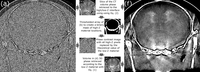
Figure 2: The masking and phase retrieval process, using a rabbit brain cross-section for demonstration. Images are labelled alphabetically according to the order in which they are computed while arrows indicate precursor images required to calculate the subsequent image. (a) A phase-contrast CT slice without any reprocessing applied, beyond flat and dark correction. (b) The same slice phase retrieved for the bone/brain tissue interface ((3)), either achieved from 3D phase retrieval of (a) or CT reconstruction of phase retrieved projections. Upon thresholding (b), we create a pixel-wise binary mask of the high-Z material, applying a dilation filter to ensure full enclosure of the high contrast boundaries. The binary mask, (c), is then used to mask all high-Z features out of the raw phase-contrast volume by replacing them with the theoretical low-Z $\mu$ value. This creates the image in (d), which is then filtered using 3D phase retrieval of the low-Z material ((2)) to make (e). Finally, the high-Z components from the interface retrieved slice (b) are spliced into (e) using the binary mask, resulting in the final phase retrieved image (f), free of over-blurring artefacts from the high-Z boundaries. All non-binary images are displayed on the same colour palette.

Imaging was performed using synchrotron radiation at $24\text{\,}\mathrm{k}\mathrm{e}\mathrm{V}$, with a $5\text{\,}\mathrm{m}$ propagation distance, and recorded using a 2048 × 2048 pixel Hamamatsu sCMOS camera (C11440-22C) with $6.5\text{\,}\mathrm{\SIUnitSymbolMicro m}$ pixel size, fibre-optically coupled to a $15\text{\,}\mathrm{\SIUnitSymbolMicro m}$ thick Gadox (Gd₂O₂S:Tb+; P43) phosphor. Due to the small width of this detector, two images from antipodal points of an offset 360 scan were stitched together to make a complete projection, with each CT then comprising 1800 projections taken at 0.1 degree increments. These CT datasets were reconstructed with a parallel beam geometry using filtered back projection [15, 16]. Material parameters of the complex refractive index were taken as $\mu=$ $55.1\text{\,}\mathrm{m}^{-1}$, $\delta=3.93\times 10^{-7}$ for material A and $\mu=$ $336.83\text{\,}\mathrm{m}^{-1}$, $\delta=5.43\times 10^{-7}$ for material B [17].

Figure 2 provides a flow diagram of all the steps required to produce the phase-retrieved output, beginning with the phase-contrast volume represented by the example CT slice in Figure 2(a). Although all stages of the method are represented via the same CT slice, we note that 3D phase retrieval is a volume operation requiring sample volumes of dimensions at least as large as the blurring kernel. In addition to the raw phase-contrast CT volume (ie. reconstructed without phase retrieval), we require a CT volume that has been phase retrieved for the A/B material interface, using Eq. 3. This volume, represented by Figure 2(b), can be calculated by phase-retrieving the phase-contrast volume in 3D [6] using (2), or by creating a new CT reconstruction from phase retrieved projections [8].

The phase-retrieved volume is used to produce a binary array of the material B locations using a simple threshold that is expanded with a 3D dilation filter to ensure all voxels containing material B are included. Figure 2(c) shows an example binary array, calculated using a threshold of $77.5\text{\,}\mathrm{m}^{-1}$ and requiring 22 iterations of a 3x3x3 kernel dilation filter due to the presence of the low absorption region (dark region) directly inside the skull. This kernel was chosen since it symmetrically expands the mask with a one pixel border; however, this could be varied as required to ensure complete coverage of all material B pixels. Using the binary array, Figure 2(c), allows material B to be masked out of the phase contrast volume, Figure 2(a), replacing the grey values of those voxels with the theoretical attenuation coefficient of the material A. This results in Figure 2(d). Previously, we attempted to remove the masked pixels using interpolation algorithms; however, even the levels of noise in the images retrieved using (3) created too much instability, causing high contrast boundaries to appear in homogeneous sample regions. Substitution of a constant value instead minimises local contrast in and near the masked region of the image and only requires prior knowledge of the low-Z material, an assumption already required by the phase retrieval algorithms. Alternatively, the replacement attenuation coefficient could be manually measured from the phase-retrieved reconstruction (Fig. 2b). Next, we apply 3D phase retrieval to the masked phase contrast volume, following (2), to produce the low-noise phase-retrieved CT volume in Figure 2(e). Having removed any high-Z material from our sample, this retrieval cannot create any over-blurring artefacts, and performing the phase retrieval in 3D additionally provides a slight SNR boost over projection-based phase retrieval [6]. Although 3D phase retrieval of large volume arrays can be RAM intensive, we were able to implement an out-of-core approach on Dell precision 5560 laptop with $32\text{\,}\mathrm{G}\mathrm{B}$ RAM, taking advantage of high SSD read and write speeds. Phase retrieval of a (1030$\times$1030$\times$1030) data volume, approximating the RAM size, was achieved in just 4.6 minutes with further avenue for optimisation. Advanced implementation on high RAM devices/computer clusters will reduce calculation times but is generally not required. After the mask threshold and dilation settings have been selected for a particular material combination, reconstructions of similar composition could be calculated consecutively without further manual intervention, providing rapid feedback during experimentation.

Finally, we use the material B binary array (Figure 2(c)) to interleave the altered regions of the 3D phase retrieved volume, Figure 2(e), with the A/B interface retrieved regions of Figure 2(b). This completes our method of 3D Masked Phase Retrieval (3DMPR), producing Figure 2(f), a low-noise CT volume that benefits from the strong phase retrieval of a low contrast material to within a few pixels of the high-Z material interface, without introducing over-blurring artefacts. This provides noise reduction within material A without eliminating features close to the A/B interface (see further examples in Section 3) and potentially allows new features of the low-Z material to be resolved that would have previously been obscured by noise.

3 Results

Using 3D phase retrieval after masking high-Z materials allows us to perform phase retrieval with strong noise suppression on complex objects to within a few pixels of highly attenuating material boundaries. This can provide contrast resolution of features previously obscured by noise or by the over-blurring of material B during the phase retrieval process.

To demonstrate the effectiveness of 3DMPR, we refer back to the data volume described in Section 2. By taking two cross-sections of the head CT volume in the sagittal plane, we compare the results of two phase retrieval approaches for the data. Figures 3(a) and 3(e) show cross sections of a standard CT reconstruction from unfiltered propagation-based phase-contrast projections, where both slices display few to no discernible brain features. Following the standard practice of Croton et. al [10], we can construct a new CT volume from projections phase retrieved to the A/B material interface, namely brain tissue-bone, using (3) (see Figures 3(b) and (f)). This allows resolution of some biological structures in the brain while others remain obscured by significant levels of noise still left in the reconstructions. Reducing the noise floor further requires stronger filtering, but merely applying phase retrieval for material A ( (1)) in projection results in over-blurring of the high contrast interface, as seen in Figures 3(c) and (g). As well as obscuring brain tissue features in direct proximity to the bone, this also disrupts the linear attenuation coefficients, making large portions of the image no longer quantitative. The method presented in this paper, producing Figures 3(d) and (h), achieves the noise reduction of stronger filtering while also retaining edge definition in the bone-brain boundary, avoiding contrast from the bone blurring into the adjacent brain tissue. Overall, we see features of the brain anatomy with greater clarity across the entire head than with the alternative reconstruction methods.

\begin{overpic}[width=107.31989pt]{3DMPR_Figure3A} \put(3.0,72.5){\shortstack[l]{{\color[rgb]{1,1,1}a)}}} \end{overpic}

\begin{overpic}[width=107.31989pt]{3DMPR_Figure3E} \put(3.0,72.5){\shortstack[l]{{\color[rgb]{1,1,1}e)}}} \end{overpic}

\begin{overpic}[width=107.31989pt]{3DMPR_Figure3B} \put(3.0,72.5){\shortstack[l]{{\color[rgb]{1,1,1}b)}}} \end{overpic}

\begin{overpic}[width=107.31989pt]{3DMPR_Figure3F} \put(3.0,72.5){\shortstack[l]{{\color[rgb]{1,1,1}f)}}} \end{overpic}

\begin{overpic}[width=107.31989pt]{3DMPR_Figure3C} \put(3.0,72.5){\shortstack[l]{{\color[rgb]{1,1,1}c)}}} \end{overpic}

\begin{overpic}[width=107.31989pt]{3DMPR_Figure3G} \put(3.0,72.5){\shortstack[l]{{\color[rgb]{1,1,1}g)}}} \end{overpic}

\begin{overpic}[width=107.31989pt]{3DMPR_Figure3D} \put(3.0,72.5){\shortstack[l]{{\color[rgb]{1,1,1}d)}}} \end{overpic}

\begin{overpic}[width=107.31989pt]{3DMPR_Figure3H} \put(3.0,72.5){\shortstack[l]{{\color[rgb]{1,1,1}h)}}} \end{overpic}

Figure 3: Comparison of our masked phase retrieval method to alternative approaches, shown using sagittal cross-sections of the rabbit head CT reconstruction volumes from Section 3. (a) and (e) are two cross-sections of the phase contrast CT as a baseline for the other algorithms. (b) and (f) are the bone-tissue interface phase-retrieved image slices, (3), showing considerable remnant noise. (c) and (g) shows the result of applying (1) phase retrieval to each projection under the assumption only brain tissue is present, leading to over-blurring completely obscuring brain tissue features in proximity to the bone. (d) and (h) are retrieved using 3DMPR to achieve an equally low SNR image whilst correctly reconstructing the A/B material interface. All images use the same colour palette.

\begin{overpic}[width=104.06787pt]{3DMPR_Figure4A} \put(3.0,85.0){\shortstack[l]{{\color[rgb]{1,1,1}a)}}} \end{overpic}

\begin{overpic}[width=104.06787pt]{3DMPR_Figure4B} \put(3.0,85.0){\shortstack[l]{{\color[rgb]{1,1,1}b)}}} \end{overpic}

\begin{overpic}[width=216.81pt]{3DMPR_Figure4C} \put(-1.0,45.0){\shortstack[l]{{\color[rgb]{0,0,0}c)}}} \end{overpic}

Figure 4: Quantification of edge resolution in a $3\text{\,}\mathrm{m}\mathrm{m}$ thick aluminium rod submerged in water after phase retrieval was applied to material A, water. (a) and (b) show slices through the aluminium cylinder from phase retrievals performed with (3) and 3DMPR, respectively. (c) Plots an azimuthally averaged line profile across the aluminium-water interface, comparing the raw phase contrast profile to that of the conventional 2D phase retrieval and our 3D masking methods. A solid vertical line is used to show the mask radius, notably not visible in (b), while a horizontal line shows the theoretical $\mu$ value of the low-Z material (water) used for replacing the masked Aluminium in the 3D reconstruction. Images (a) and (b) share the same colour palette.

3.1 SNR Characterisation

Accurately measuring SNR gains in complex samples is difficult since variations in sample composition across measurement areas can be incorrectly attributed to noise. Additionally, 3D phase retrieval ordinarily provides a slight SNR boost over 2D, projection-based phase retrieval [6], giving the masked retrieval approach an advantage. To provide a valid and equivalent comparison of the two methods we measured noise characteristics of the brain tissue data using a large area within the skull of the phase contrast data, Figure 3(a) and (e), where noise dominates any mean variation in the linear attenuation coefficient. This was measured to be $\mu=55.071\pm 49.049$, giving an SNR of 1.123. A $1000\times 1000\times 1000$ data volume was then created to match the brain tissue noise level and emulate a CT volume only containing brain tissue. 3D phase retrievals were then applied to the volume using the A/B interface in (3) and to material A using (1), and the whole volume analysed, creating a comparison of the 2D phase retrieval with (3) to 3DMPR. Phase retrieving to the A/B interface increases SNR to 114.3, while phase retrieving for material A alone, as in the masked phase retrieval method gives, an SNR of 888.2; 6.9 times higher while maintaining the same edge resolution between bone and brain tissue.

3.2 Boundary Preservation

To quantify the method’s ability to preserve high contrast material boundaries, and the amount of over-blurring it avoids, we explore the simple and well-characterised dataset of an aluminium pin submerged in water. This dataset was recorded on a $50\text{\,}\mathrm{\SIUnitSymbolMicro m}$ pixel Hamamatsu CMOS flat panel detector (C9728DK-10) using a microfocus X-ray source (THE-Plus from X-RAY WorX, Gmbh) with a silver transmission target at a tube voltage of $35\text{\,}\mathrm{k}\mathrm{V}_{\mathrm{p}}$. The mean X-ray energy was determined by comparing $\mu$ values of water measured in CT at the radial depth of the aluminum pin, resulting in a mean energy of $19.58\text{\,}\mathrm{k}\mathrm{e}\mathrm{V}$. The source-to-object distance was $0.96\text{\,}\mathrm{m}$ with the source-to-detector distance set to $2.40\text{\,}\mathrm{m}$, resulting in a 2.50 times magnification and effective propagation distance of $0.576\text{\,}\mathrm{m}$. CTs were reconstructed with 3,271 projections at 0.11 degree increments using filtered back projection in a fan beam geometry[15, 16]. For this sample, material A is taken to be water, $\mu=$ $84.72\text{\,}\mathrm{m}^{-1}$ and $\delta=6.00\times 10^{-7}$, while material B is the comparatively high-Z aluminium, $\mu=$ $985.86\text{\,}\mathrm{m}^{-1}$ and $\delta=1.42\times 10^{-9}$ [17].

Figure 4 shows example portions of a CT slice through the aluminium pin for phase retrieval (a) with (1) and (b) with our 3DMPR method. Each figure applies the same filtering to regions surrounding the aluminium cylinder, but (b) uses interface-tuned phase retrieval to more accurately preserve the A/B material boundary. For 3DMPR, the aluminium cylinder was masked using a $\mu$ threshold of $300\text{\,}\mathrm{m}^{-1}$ with two iterations of a 3$\times$3$\times$3 dilation filter. Despite the aluminium insert having uniform density, both figures 4(a) and (b) show a decrease in attenuation coefficient toward the centre, which is a cupping artefact caused by beam hardening. This results from variable penetration depths of the polychromatic X-ray spectrum [10]. Figure 4(c) plots azimuthally-averaged line profiles across the A/B boundary in (a) and (b), incorporating the phase contrast profile from the non-phase-retrieved CT slice for comparison. A solid vertical line represents the edge of the mask used for replacing the material B. The horizontal dashed line denotes the theoretical linear attenuation coefficient value used for the temporary high-Z replacement, calculated using the mean energy of the polychromatic source, which closely resembles the measured linear attenuation coefficient outside the region being replaced. Figure 4(c) shows the edge profile of our 3DMPR most closely resembles the true boundary interface of the aluminium pin, whereas the (1) phase retrieval shows a very low-contrast, blurred edge due to over-blurring, even when retrieving at a relatively small effective propagation distance of $0.576\text{\,}\mathrm{m}$. This over-blurring leaves the area about the boundary unsuitable for quantitative analysis, even for any features of interest not obscured by the edge blurring. To measure the blurring extent of each approach, we numerically differentiated each edge profile and applied a Pearson VII fit to determine the full width at half maxima [10]. Pearson VII functions are appropriate fits for point spread functions (PSFs) [10] since they have freedom that enable their shape to lie on a spectrum between Lorentzian and Gaussian. Through this convention, the spatial resolution of the conventional phase-retrieval approach was found to be $108\pm 2\text{\,}\mathrm{\SIUnitSymbolMicro m}$, while our approach was measured at $54\pm 1\text{\,}\mathrm{\SIUnitSymbolMicro m}$. This demonstrates a clear improvement in material boundary definition while retaining the same SNR boost in the low-Z material of $4.2\times$, measured using the same method described in Section 3A. This SNR boost will be particularly valuable in improving weakly-attenuating feature resolution in low flux imaging scenarios.

\begin{overpic}[width=69.38078pt]{3DMPR_Figure5A} \put(3.0,82.5){\shortstack[l]{{\color[rgb]{1,1,1}a)}}} \end{overpic}

\begin{overpic}[width=143.09538pt,height=69.38078pt]{3DMPR_Figure5B} \put(-2.0,42.5){\shortstack[l]{{\color[rgb]{0,0,0}b)}}} \put(31.0,35.0){\shortstack[l]{{\color[rgb]{0,0,0}x}}} \put(68.0,27.0){\shortstack[l]{{\color[rgb]{0,0,0}y}}} \put(86.0,21.0){\shortstack[l]{{\color[rgb]{0,0,0}z}}} \end{overpic}

\begin{overpic}[width=69.38078pt]{3DMPR_Figure5C} \put(3.0,82.5){\shortstack[l]{{\color[rgb]{1,1,1}c)}}} \end{overpic}

\begin{overpic}[width=69.38078pt]{3DMPR_Figure5D} \put(3.0,82.5){\shortstack[l]{{\color[rgb]{1,1,1}d)}}} \end{overpic}

\begin{overpic}[width=69.38078pt]{3DMPR_Figure5E} \put(3.0,82.5){\shortstack[l]{{\color[rgb]{1,1,1}e)}}} \end{overpic}

\begin{overpic}[width=69.38078pt]{3DMPR_Figure5F} \put(3.0,82.5){\shortstack[l]{{\color[rgb]{1,1,1}f)}}} \end{overpic}

\begin{overpic}[width=69.38078pt]{3DMPR_Figure5G} \put(3.0,82.5){\shortstack[l]{{\color[rgb]{1,1,1}g)}}} \end{overpic}

\begin{overpic}[width=69.38078pt]{3DMPR_Figure5H} \put(3.0,82.5){\shortstack[l]{{\color[rgb]{1,1,1}h)}}} \end{overpic}

\begin{overpic}[width=69.38078pt]{3DMPR_Figure5I} \put(3.0,82.5){\shortstack[l]{{\color[rgb]{1,1,1}i)}}} \end{overpic}

\begin{overpic}[width=69.38078pt]{3DMPR_Figure5J} \put(3.0,82.5){\shortstack[l]{{\color[rgb]{1,1,1}j)}}} \end{overpic}

Figure 5: The masking and phase retrieval process conceptualised for the multi-material CT slice, composed of materials x,y and z as shown in (a), under the assumption of contrast isolation between all materials as in the histogram (b). Dashed, vertical lines demonstrate example threshold bounds for creating material masks, shown in (c)(d)(e). The inverse of theses masks, black regions, can be used to mask away all other material components, allowing phase retrieval to be performed to internal material regions using (1). The boundary regions are interleaved from appropriately tuned retrievals, located using binary operations between the material masks after an additional dilation (f)(g)(h). (i) shows the result of a binary ’and’ operation between the material x and y masks, creating a trace of the x/y interface for interleaving. (j) demonstrates the same for the y/z interface, overcoming the convention limit of two-way material boundaries.

3.3 Expansion to 3+ Material Interfaces

While section 2 demonstrated the 3DMPR process using a two material sample, here we generalise to higher sample compositions and demonstrate how masked phase retrieval may be used to overcome a restriction of the two-material algorithm of (3). The phase-retrieval algorithms of (1) and (3) require that each material is only in contact with a maximum of one other material or vacuum. Otherwise, only parts of the material’s boundary will be quantitatively reconstructed.

Phantoms containing relevant information in multiple attenuation levels adjacent to high-Z boundaries are uncommon in medicine; therefore, to demonstrate the concept we consider a mock 3-material CT slice, shown in Figure 5(a), composed of materials x, y, and z and possessing 4 unique interfaces: x/air, x/y, x/z and y/z. Phase retrieval with the two-material algorithm (Eq. 3) cannot fully resolve the boundary of any material. For example, phase retrieval focused on the y/x interface will leave the y/z interface non-quantitative. Our approach relaxes the requirement for spatially-isolated materials but does require materials to be contrast-resolved, as in the histogram of Figure 5(b). This allows two-sided thresholding to create binary masks for each material, Figures 5(c,d,e), in place of the single-sided thresholding used in Section 2. Alternatively, material segmentation may be performed through region-growing algorithms or other advanced processes. Materials with overlapping $\mu$ distributions may share equivalent enough phase characteristics to be considered a single material, allowing the characteristics of either material to be used in place of the other or an average of both to be used.

3DMPR is then divided into two categories; the relatively constant regions within each material, termed homogeneous regions, and regions around material boundaries containing two materials, referred to as heterogeneous. Phase retrieval to homogeneous regions is performed to the CT volume, using equation (1), after replacing all other image components with the theoretical material value using the inverse of masks (Figure 5(c), (d) and (e)). A dilation filter may be required on the inverse masks to ensure heterogeneous regions are not included. When combined, these reconstructions provide strong noise suppression within each material, without over-blurring low-Z components, but do not yet include the material boundaries. These heterogeneous sample regions must be interleaved from appropriately tuned reconstructions, requiring knowledge of the boundary locations, acquired through further manipulation of the binary masks (Figures 5(c, d, e)). The masks are expanded by an equivalent amount via dilation filters (Figures 5(f, g, h)) until masks of adjacent materials overlap. Binary ‘and’ operations are then used to isolate the overlapping regions which will be centred about the material boundaries. Figures 5(i) and (j) show examples of this for the y-x and y-z material interfaces, respectively, which can then be used to select these regions from the appropriate reconstructions.

Interleaving all homogeneous and heterogeneous regions together, and iterating the method proven in Sections 2, 3a and 3b, will produce a noise suppressed CT reconstruction with quantitative resolution at all material boundaries.

4 Conclusion

We present a method for achieving strong noise reduction during phase retrieval of multi-material objects, without creating over-blurring along material boundaries with high-Z materials. By using simple thresholding techniques for material isolation in CT, the method is computationally efficient with run-times in the order of minutes when both input and output Fourier transform arrays are smaller than the system RAM. A rabbit kitten brain CT was used to demonstrate the method’s computational process and ability to improve image quality in complex, biological samples. SNR values increased from 1.123 in the phase contrast images to 888.2 using 3DMPR, an increase of 6.9 times over the two-material phase retrieval algorithm, whilst preserving the same boundary definition between the high and low-Z materials. Conversely, when SNR gain was maintained in a separate, well-characterised dataset, edge resolution across the high-Z boundary fell to $108\pm 2\text{\,}\mathrm{\SIUnitSymbolMicro m}$ using the approach in (3), compared to $54\pm 1\text{\,}\mathrm{\SIUnitSymbolMicro m}$ with the new approach. This method will allow strong SNR-boosting phase retrieval to be applied to a wider range of multi-material objects.

Data Availability Statement

The datasets used and/or analysed for this manuscript are available from the corresponding author on reasonable request.

References

- [1] Rozemarijn Vliegenthart, Andreas Fouras, Colin Jacobs, and Nickolas Papanikolaou. Innovations in thoracic imaging: CT, radiomics, AI and x-ray velocimetry. Respirology (Carlton, Vic.), 27(10):818–833, October 2022.
- [2] Marcus J. Kitchen, Genevieve A. Buckley, Timur E. Gureyev, Megan J. Wallace, Nico Andres-Thio, Kentaro Uesugi, Naoto Yagi, and Stuart B. Hooper. CT dose reduction factors in the thousands using X-ray phase contrast. Scientific Reports, 7(1):15953, November 2017. Number: 1 Publisher: Nature Publishing Group.
- [3] Benedicta D. Arhatari, Yakov I. Nesterets, Seyedamir T. Taba, Anton Maksimenko, Christopher J. Hall, Andrew W. Stevenson, Daniel Häsermann, Sarah J. Lewis, Matthew Dimmock, Darren Thompson, Sheridan C. Mayo, Harry M. Quiney, Timur E. Gureyev, and Patrick C. Brennan. X-ray phase-contrast computed tomography for full breast mastectomy imaging at the Australian Synchrotron. In Developments in X-Ray Tomography XIII, volume 11840, page 131. SPIE, September 2021.
- [4] Timur E. Gureyev, Yakov I. Nesterets, Alexander Kozlov, David M. Paganin, and Harry M. Quiney. On the “unreasonable” effectiveness of transport of intensity imaging and optical deconvolution. JOSA A, 34(12):2251–2260, December 2017. Publisher: Optica Publishing Group.
- [5] D. Paganin, S. C. Mayo, T. E. Gureyev, P. R. Miller, and S. W. Wilkins. Simultaneous phase and amplitude extraction from a single defocused image of a homogeneous object. Journal of Microscopy, 206(Pt 1):33–40, April 2002.
- [6] Darren A. Thompson, Yakov I. Nesterets, Konstantin M. Pavlov, and Timur E. Gureyev. Fast three-dimensional phase retrieval in propagation-based X-ray tomography. Journal of Synchrotron Radiation, 26(Pt 3):825–838, May 2019.
- [7] Mario Beltran, David Paganin, Karen Siu, Andreas Fouras, Stuart Hooper, David Reser, and Marcus Kitchen. Interface-specific x-ray phase retrieval tomography of complex biological organs. Physics in Medicine & Biology, 56(23):7353–7369, 2011. Publisher: IOP Publishing.
- [8] M. A. Beltran, D. M. Paganin, K. Uesugi, and M. J. Kitchen. 2D and 3D X-ray phase retrieval of multi-material objects using a single defocus distance. Optics Express, 18(7):6423–6436, March 2010. Publisher: Optica Publishing Group.
- [9] Linda Croton, Kaye Morgan, David Paganin, Lauren Kerr, Megan Wallace, Kelly Crossley, Gary Ruben, Suzanne Miller, Naoto Yagi, Kentaro Uesugi, Stuart Hooper, and Marcus Kitchen. Imaging the Brain In Situ with Phase Contrast CT. Microscopy and Microanalysis, 24(S2):352–353, August 2018. Publisher: Cambridge University Press.
- [10] Linda C. P. Croton, Kaye S. Morgan, David M. Paganin, Lauren T. Kerr, Megan J. Wallace, Kelly J. Crossley, Suzanne L. Miller, Naoto Yagi, Kentaro Uesugi, Stuart B. Hooper, and Marcus J. Kitchen. In situ phase contrast X-ray brain CT. Scientific Reports, 8(1):11412, July 2018. Number: 1 Publisher: Nature Publishing Group.
- [11] Lorenz Hehn, Kaye Morgan, Pidassa Bidola, Wolfgang Noichl, Regine Gradl, Martin Dierolf, Peter B. Noël, and Franz Pfeiffer. Nonlinear statistical iterative reconstruction for propagation-based phase-contrast tomography. APL Bioengineering, 2(1):016105, March 2018. Publisher: American Institute of Physics.
- [12] Lorenz Hehn, Regine Gradl, Andrej Voss, Benedikt Günther, Martin Dierolf, Christoph Jud, Konstantin Willer, Sebastian Allner, Jörg U. Hammel, Roland Hessler, Kaye S. Morgan, Julia Herzen, Werner Hemmert, and Franz Pfeiffer. Propagation-based phase-contrast tomography of a guinea pig inner ear with cochlear implant using a model-based iterative reconstruction algorithm. Biomedical Optics Express, 9(11):5330–5339, November 2018. Publisher: Optica Publishing Group.
- [13] C. T. Chantler, K. Olsen, R. A. Dragoset, J. Chang, A. R. Kishore, S. A. Kotochigova, and D. S. Zucker. X-Ray Form Factor, Attenuation, and Scattering Tables. NIST, 2005.
- [14] M. J. Berger, J. H. Hubbell, S. M. Seltzer, J. Chang, J. S. Coursey, R. Sukumar, D. S. Zucker, and K. Olsen. XCOM: Photon Cross Sections Database. NIST, 2010.
- [15] Wim van Aarle, Willem Jan Palenstijn, Jeroen Cant, Eline Janssens, Folkert Bleichrodt, Andrei Dabravolski, Jan De Beenhouwer, K. Joost Batenburg, and Jan Sijbers. Fast and flexible X-ray tomography using the ASTRA toolbox. Optics Express, 24(22):25129–25147, October 2016. Publisher: Optica Publishing Group.
- [16] Wim van Aarle, Willem Jan Palenstijn, Jan De Beenhouwer, Thomas Altantzis, Sara Bals, K. Joost Batenburg, and Jan Sijbers. The ASTRA Toolbox: A platform for advanced algorithm development in electron tomography. Ultramicroscopy, 157:35–47, October 2015.
- [17] Tom Schoonjans, Antonio Brunetti, Bruno Golosio, Manuel Sanchez del Rio, Vicente Armando Solé, Claudio Ferrero, and Laszlo Vincze. The xraylib library for X-ray–matter interactions. Recent developments. Spectrochimica Acta Part B: Atomic Spectroscopy, 66(11):776–784, November 2011.