Sample Efficient Deep Reinforcement Learning via Local Planning

Abstract

The focus of this work is sample-efficient deep reinforcement learning (RL) with a simulator. One useful property of simulators is that it is typically easy to reset the environment to a previously observed state. We propose an algorithmic framework, named uncertainty-first local planning (UFLP), that takes advantage of this property. Concretely, in each data collection iteration, with some probability, our meta-algorithm resets the environment to an observed state which has high uncertainty, instead of sampling according to the initial-state distribution. The agent-environment interaction then proceeds as in the standard online RL setting. We demonstrate that this simple procedure can dramatically improve the sample cost of several baseline RL algorithms on difficult exploration tasks. Notably, with our framework, we can achieve super-human performance on the notoriously hard Atari game, Montezuma’s Revenge, with a simple (distributional) double DQN. Our work can be seen as an efficient approximate implementation of an existing algorithm with theoretical guarantees, which offers an interpretation of the positive empirical results.

1 Introduction

Simulators are ubiquitous in modern reinforcement learning (RL). They correspond to either to the environment itself (as in chess, go, and video games (Bellemare et al., 2013)) or to a simplified model of the true environment (such as robotic arm manipulation (Qassem et al., 2010; Akkaya et al., 2019), car driving (Bojarski et al., 2016; Aradi, 2020), or plasma shape control in fusion (Degrave et al., 2022)). Simulators have been widely used in RL research. Many standard benchmarks in RL involve simulators, for example, Atari games (Bellemare et al., 2013), Mujoco simulation engine (Todorov et al., 2012), OpenAI Gym (Brockman et al., 2016), DeepMind control suite (Tassa et al., 2018), and DeepMind Lab (Beattie et al., 2016). Somewhat surprisingly, the majority of RL algorithms use the agent-environment interaction protocols that mimic learning in the real world during training, and do not explicitly take advantage of favorable simulator properties. In particular, the standard interaction protocol, called online access, assumes that the agent can only follow the dynamics of the environment during learning. In this work, we consider the local access protocol (Yin et al., 2022), where the agent is allowed to revisit any previously observed state in addition to following the dynamics. This protocol can easily be implemented with simulators for many commonly used RL environments (see, e.g., Appendix B).

Local access has received less attention from the RL community compared online access. On the theory side, several recent works show that local access makes sample-efficient learning possible in settings where it has not been shown in the online access setting (Li et al., 2021; Yin et al., 2022; Hao et al., 2022). On the empirical side, the vine method in TRPO (Schulman et al., 2015) uses local access to obtain better estimates of the value function, and the Go-Explore algorithm of Ecoffet et al. (2019) relies on local access to achieve state-of-the-art performance on several hard-exploration Atari games. Intuitively, the main advantage of local access is that we can directly reset the simulator to the states that can provide more information to the agent, and thus improve the exploration of the state space.

Contributions

Our contribution is three-fold:

• We propose a general algorithmic framework for RL with a simulator under the local access protocol. Our framework, named uncertainty-first local planning (UFLP), revisits states from the agent’s history based on the uncertainty about their value.

• We instantiate this framework with several base RL agents (deep Q-networks, policy iteration) and uncertainty estimates (ensemble, feature covariance, approximate counts, random network distillation).

• We demonstrate that UFLP can significantly improve the sample cost compared to online access on difficult exploration tasks, including the Deep Sea and Cartpole Swingup benchmarks in bsuite (Osband et al., 2019) and hard-exploration Atari games: Montezuma’s Revenge and PrivateEye. In particular, for the Deep Sea environment, by leveraging UFLP, many RL agents can easily solve the task, whereas in the online access setting they can only obtain zero reward. For Montezuma’s Revenge, applying UFLP on top of a simple double DQN (Van Hasselt et al., 2016) results in a super-human score.

Our work also opens up a new research avenue for improving sample efficiency when learning with simulators.

2 Related Work

Local access protocol

Simulators are routinely used in RL algorithms that leverage Monte Carlo tree search (Coulom, 2006; Kocsis and Szepesvári, 2006), including prominent examples such as AlphaGo (Silver et al., 2016) and AlphaZero (Silver et al., 2018). One major difference between the tree-search setting and the setting that we consider in this paper is that the tree-search algorithms usually make the assumption that the agent has local access to the simulator during evaluation, whereas we only consider local access during training. This means that once the training is finished, the agent is evaluated against the environment without access to the simulator. Therefore, our framework is more suitable for applications that require fast inference when the agent is deployed. Moreover, most tree-search approaches do not select states to revisit strategically; instead, they expand the search tree based on visitation counts, rather than more general uncertainty metrics.

One notable example of RL with local access protocol is the Go-Explore algorithm (Ecoffet et al., 2019, 2021). This algorithm operates under the local access protocol and revisits states deemed to be “promising” in history. It then uses backward learning-from-demonstrations (Salimans and Chen, 2018) to learn a robust policy. While Go-Explore achieves or surpasses the state of the art on $11$ Atari games, the algorithm design, especially the state revisiting rule, uses heuristics tailored to these games, and it is unclear how to combine this method with other uncertainty metrics or more general RL agents. By contrast, in this paper, we propose a general algorithm framework that can be combined with most existing RL agents in order to improve their performance.

Besides Go-Explore, a few other prior works have studied the use of local access. In an early literature on real-time dynamic programming (Barto et al., 1995; McMahan et al., 2005; Smith and Simmons, 2006; Sanner et al., 2009), it has been shown that prioritizing revisiting states with higher uncertainty is helpful for achieving faster convergence. However, these works mainly focus on tabular MDPs and only consider the value iteration algorithm. On the contrary, our general framework is suitable for function approximation and can be combined with other types of agents beyond value iteration. In the vine method in the TRPO algorithm (Schulman et al., 2015), local access is used to obtain more accurate estimates of the value function. This differs from our work since we focus on improving exploration of deep RL agents. Restart distributions have also been explored in Tavakoli et al. (2019), who consider revisiting states uniformly at random, according to TD error, and according to episode returns, in combination with the PPO algorithm (Schulman et al., 2017). Revisiting based on high episode returns improves the performance of PPO on a sparse-reward task deemed hard-exploration. However, it is unclear that the same approach would be successful in environments such as Deep Sea (Osband et al., 2019), where discovering an episode with a positive return requires non-trivial exploration. A very recent work by Lan et al. (2023) focuses on generalization of RL agents to out-of-distribution trajectories using local access to a simulator. Their algorithm can be considered as a special case in our framework.

On the theoretical side, several recent works have proposed sample- and computationally-efficient algorithms under the local access protocol and with linearly-realizable action-value functions (Li et al., 2021; Yin et al., 2022; Hao et al., 2022; Weisz et al., 2022). The works of Yin et al. (2022), Hao et al. (2022), and Weisz et al. (2022) maintain a core set of previously-visited states that cover different parts of the feature space. In the online access setting, a similar idea is used in the policy cover policy gradient (PCPG) algorithm of Agarwal et al. (2020) and the follow-up work of Zanette et al. (2021). Our work is motivated by the approaches of Yin et al. (2022) and Hao et al. (2022), but adapted to the practical setting of value learning with neural network function approximation, where the core set is more difficult to define rigorously.

Uncertainty estimation and exploration in RL

Successful methods for learning in MDPs typically rely on estimates of uncertainty about the value of state-action pairs in order to encourage the agent to explore the environment. One type of exploration strategies rely on uncertainty-based intrinsic rewards or bonuses. Uncertainty metrics based on feature covariance have been used in theoretical RL works with linear function approximation (Jin et al., 2020). Empirically, popular approaches include approximate count (Tang et al., 2017; Bellemare et al., 2016), random network distillation (RND) (Burda et al., 2018), and curiosity-driven exploration (Pathak et al., 2017). Recent successful approaches (Badia et al., 2020b, a) have constructed bonuses based on nearest-neighbors in the current episode, as well as RND to capture longer-term uncertainty. Another set of approaches rely on randomized value functions (Osband et al., 2016, 2018). We discuss these methods in more detail in Section 5.1.

3 Problem Setting

We use $\Delta_{\mathcal{S}}$ to denote the set of probability distributions defined on any countable set $\mathcal{S}$ and write $[N]:=\{1,2,\ldots,N\}$ for any positive integer $N$.

An infinite-horizon discounted Markov decision process (MDP) can be characterized by a tuple $(\mathcal{S},\mathcal{A},R,P,\mu_{0},\gamma)$, where $\mathcal{S}$ is the state space, $\mathcal{A}$ is the action space, $R:\mathcal{S}\times\mathcal{A}\rightarrow[0,1]$ is the reward function, $P:\mathcal{S}\times\mathcal{A}\rightarrow\Delta_{\mathcal{S}}$ is the probability transition kernel, $\mu_{0}$ is the initial state distribution, and $\gamma\in(0,1)$ is the discount factor. Both $P$ and $R$ are unknown. In this paper, we only consider finite action space $|\mathcal{A}|<\infty$.

At each state $s$, if the agent picks an action $a\in\mathcal{A}$, the environment evolves to a random next state $s^{\prime}$ according to the distribution $P(s^{\prime}|s,a)$ and generates a stochastic reward $r\in[0,1]$ with $\mathbb{E}[r|s,a]=R(s,a)$.

A stationary policy $\pi:\mathcal{S}\rightarrow\Delta_{\mathcal{A}}$ is a mapping from a state to a distribution over actions. For a policy $\pi$, its value function $V_{\pi}(s)$ is the expectation of cumulative rewards received under policy $\pi$ when starting from a state $s$, i.e., $V_{\pi}(s)=\mathbb{E}^{\pi}\left[\sum_{t=0}^{\infty}\gamma^{t}R(s_{t},a_{t})\Big{|}s_{0}=s\right]$, where $a_{t}\sim\pi(\cdot|s_{t}),s_{t+1}\sim P(\cdot|s_{t},a_{t})$ and $\mathbb{E}^{\pi}$ denotes the expectation over the sample path and stochastic reward generated under policy $\pi$. The action value function $Q_{\pi}(s,a)$ is defined as $Q_{\pi}(s,a)=\mathbb{E}^{\pi}\left[\sum_{t=0}^{\infty}\gamma^{t}R(s_{t},a_{t})\Big{|}s_{0}=s,a_{0}=a\right]$.

3.1 Simulator Interaction Protocol

We distinguish between three protocols for interacting with the MDP simulator (or environment) commonly used in the literature.

• Online access. The initial state $s_{0}$ is sampled from the initial state distribution $\mu_{0}$. The agent can only reset the environment to a (possibly random) initial state, or move to the next state given an action by following the MDP dynamics.

• Local access. The agent can reset the environment to a random initial state, or to a state that has previously been observed.

• Random access. The agent can query the simulator with any state-action pair of its choice to obtain a reward and a sample of the next state. This is often referred as the access to a generative model in literature (Kakade, 2003; Sidford et al., 2018; Yang and Wang, 2019).

Most RL algorithms use the online access protocol, which also mimics learning in the real world. Random access is primarily considered in theoretical works, as it enables sample-efficient learning in settings where this is impossible under online access (Du et al., 2020). Unfortunately, this interaction protocol is often difficult or impossible to support in large-scale MDPs where the agent may not even know which states exist or are plausible. For example, for random access, the agent would need to know which positions and velocities of a robotic arm are valid according to physics, or which images correspond to a valid frame of a video game. The local access protocol does not suffer from this issue, as the agent is only allowed to revisit previously observed states which are known to be plausible. Local access is also easy to implement in most simulators, for example by checkpointing the simulator state.

The intuition on why using local access can improve sample efficiency of policy optimization is that we can directly reset the simulator to the states that can provide more information to the agent. In other words, we can directly start data collection from the states with high uncertainty. In the online access mode, exploration methods such as additive bonus and Thompson sampling (Thompson, 1933; Osband et al., 2016) have been designed to achieve the similar goal; however, in this setting, the agent still has to start from the initial state, reach an uncertain state, and then collect data there. Therefore, local access saves the sample cost by leveraging the resetting ability of simulators.

4 Algorithm Framework

In this section, we present an algorithm framework for policy optimization with local access to a simulator. There are four main components in our framework:

• A simulator (or environment) that we can reset to any state that has been observed during the learning process, denoted by Env in the following. We denote the operation of resetting the environment to a given observed state $s$ by $\texttt{Env}.\textsc{Reset}(s)$. We also denote the operation of stepping the environment (taking an action and moving to the next state) by $\texttt{Env}.\textsc{Step}(a)$.

• A base agent (Agent) that can take actions given the observation of a state $s$ ($\texttt{Agent}.\textsc{Act}(s)$) and update itself ($\texttt{Agent}.\textsc{Update}()$) given collected data. In fact, any agent for online-access RL can be used as a base agent in our framework.

• A function $u:\mathcal{S}\times\mathcal{A}\mapsto\mathbb{R}$ that measures the uncertainty of the agent about the value of state-action pairs. In some cases, we only define the uncertainty of the states, i.e., $u:\mathcal{S}\mapsto\mathbb{R}$. This function is are typically updated during learning.

• A history buffer $\mathcal{H}$. Each element in $\mathcal{H}$ contains all the necessary information to reset the environment to a particular state $s$. Note that the history buffer differs from the replay buffer, which is usually used to maintain state-action transition tuples and update the agent. In the following, we omit the role of the replay buffer and mainly focus on the use of the history buffer.

Similarly to online access, our framework includes a data collection process, where the agent interacts with the environment and collects data, and a learning process where the agent is updated. The major difference in our framework is that we need to specify a starting state-action pair in the data collection process; more specifically, we reset the simulator to a given state, take a given action, move to the next state and follow the agent’s action selection afterwards. This process, denoted by $\textsc{DataCollection}(\texttt{Env},\texttt{Agent},s_{0},a_{0},\mathcal{H})$ is described in Algorithm 1.

Algorithm 1 $\textsc{DataCollection}(\texttt{Env},\texttt{Agent},s_{0},a_{0},\mathcal{H})$

Input: environment Env, base agent Agent, starting state-action $s_{0},a_{0}$, history buffer $\mathcal{H}$.

  $\mathcal{H}\leftarrow\mathcal{H}\cup\{s_{0}\}$

  $\texttt{Env}.\textsc{Reset}(s_{0})$

  $s\leftarrow\texttt{Env}.\textsc{Step}(a_{0})$

  while end of episode not reached do

     $\mathcal{H}\leftarrow\mathcal{H}\cup\{s\}$

     $a\leftarrow\texttt{Agent}.\textsc{Act}(s)$

     $s\leftarrow\texttt{Env}.\textsc{Step}(a)$

  end while

With these components, we are ready to present our algorithm framework, uncertainty-first local planning (UFLP). Here, we use the term planning to distinguish our learning setting from the online access mode where data must be collected episode-by-episode during training. In UFLP, in each data collection iteration, with probability $p_{\text{init}}\in[0,1]$, we sample an initial state $s_{0}$ according to the initial state distribution $\mu_{0}$ and start data collection from $s_{0}$. Otherwise, we sample a batch of $B$ elements from the history buffer $\mathcal{H}$, denoted by $\mathcal{H}_{B}$, pair these states with all possible actions, and choose the highest-uncertainty state-action pair as the starting point, i.e., we choose the starting point according to

$$s_{0},a_{0}\leftarrow\operatorname*{arg\,max}_{s\in\mathcal{H}_{B},a\in\mathcal{A}}u(s,a).$$ (1)

As we can see, if $p_{\text{init}}=1$, the algorithm reduces to the online access mode. We present details of our framework in Algorithm 2, where we use $\rm{Unif}[0,1]$ to denote a random number that is sampled uniformly at random from $[0,1]$.

Algorithm 2 UncertaintyFirstLocalPlanning

Inputs: environment Env, base agent Agent, probability of starting from initial state $p_{\text{init}}\in[0,1]$, history buffer batch size $B$, uncertainty metric $u$.

  $\mathcal{H}\leftarrow\emptyset$

  while termination criteria not met do

     if ${\rm Unif}[0,1]\leq p_{\text{init}}$ or $\mathcal{H}=\emptyset$ then

        Get $s_{0}\sim\mu_{0}$, $a_{0}\leftarrow\texttt{Agent}.\textsc{Act}(s_{0})$

     else

        Sample $B$ elements from $\mathcal{H}$, denoted by $\mathcal{H}_{B}$.

        $s_{0},a_{0}\leftarrow\operatorname*{arg\,max}_{s\in\mathcal{H}_{B},a\in\mathcal{A}}u(s,a)$

     end if

     $\textsc{DataCollection}(\texttt{Env},\texttt{Agent},s_{0},a_{0},\mathcal{H})$

     Agent.Update()

  end while

One intuition behind the criterion that chooses an uncertain state as a starting point is that it expands the subset of the state space that we can use to start the data collection process, which in turn helps control extrapolation errors in value function estimation. Revisiting uncertain states can also improve sample efficiency in environments where states that are important for decision-making are difficult to reach.

We also note that in practice, storing all the states that the agent has visited during training may require too much memory. Therefore, we implement the history buffer $\mathcal{H}$ using a FIFO queue. Another note is that if we only have an uncertainty metric for states rather than state-action pairs, we can choose the most uncertain state in $\mathcal{H}_{B}$ and pair it with a random action, i.e.,

$$s_{0}\leftarrow\operatorname*{arg\,max}_{s\in\mathcal{H}_{B}}u(s),\leavevmode\nobreak\ a_{0}\sim\rm{Unif}(\mathcal{A}).$$ (2)

Our experiments in Section 6.1 for bsuite environments (Osband et al., 2019) use Eq. 1 and those in Section 6.2 for Atari games (Bellemare et al., 2013) use Eq. 2.

Next, we describe several instantiations of base agents and uncertainty metrics that can be used with the local access protocol.

5 Base Agents and Uncertainty Metrics

5.1 Base Agents

For base agents, we consider the following commonly used ones: double deep Q network (DDQN) (Van Hasselt et al., 2016), bootstrapped DDQN (BootDDQN) (Osband et al., 2016, 2018), distributional DDQN (Bellemare et al., 2017), and approximate policy iteration (PI) (Bertsekas, 2011).

DDQN

Double DQN is an improvement of the original DQN agent by Mnih et al. (2015). In DDQN, the agent is updated by minimizing the following loss over the transition tuples of the form $(s_{t},a_{t},r_{t},s_{t+1})$ sampled from the replay buffer $\mathcal{R}$:

$$L_{\text{DDQN}}(\theta)=\mathbb{E}_{\mathcal{R}}\big{(}Q(s_{t},a_{t};\theta)-r_{t}-\gamma Q(s_{t+1},\arg\max_{a\in\mathcal{A}}Q(s_{t+1},a;\theta);\theta^{\prime})\big{)}^{2},$$ (3)

where $\theta$ denotes the parameters of the Q-network, and $\theta^{\prime}$ denotes the parameters of the target network that is periodically updated. During acting, one can use the standard $\epsilon$-greedy strategy, where with probability $\epsilon$, we take a random action, and otherwise we act greedily w.r.t. $Q(s,a;\theta)$.

To improve exploration, one can use an additive bonus, a.k.a. optimism. There are two common approaches. First, adding an acting-time bonus means that we fit the Q-network using Eq. 3 and select actions according to

$$\textsc{Act}(s)=\arg\max_{a\in\mathcal{A}}Q(s,a;\theta)+cu(s,a),$$ (4)

where $u(s,a)$ is the uncertainty metric and $c>0$ is a scaling factor. A similar approach has been discussed in Chen et al. (2017). The second approach is to add an intrinsic reward to the reward $r_{t}$ provided by the environment, i.e., replace $r_{t}$ in Eq. 3 with

$$r^{\prime}_{t}=r_{t}+cu(s_{t},a_{t})$$ (5)

and train the Q-network with $r^{\prime}_{t}$. This approach has been widely used in the literature (Tang et al., 2017; Bellemare et al., 2016; Badia et al., 2020b). In the following, we call the DDQN agent with acting-time bonus and intrinsic reward DDQN-Bonus and DDQN-Intrinsic, respectively.

Bootstrapped DDQN

Another approach to improving exploration of the DQN agent is to mimic the behavior of Thompson sampling (Thompson, 1933). Osband et al. (2016) proposed the boostrapped DQN agent to achieve this goal. Here we replace the DQN loss with the DDQN loss in Eq. 3 and thus we name this agent bootstrapped DDQN (BootDDQN). This agent maintains an ensemble of $M$ Q-networks. For the $m$-th network, the parameters are a summation of a trainable component $\theta_{m}$ and a fixed randomized prior (Osband et al., 2018) network $\theta_{m}^{p}$, and thus the Q-network can be denoted by $Q(s,a;\widetilde{\theta}_{m})$, where $\widetilde{\theta}_{m}:=\theta_{m}+\theta_{m}^{p}$. The randomized prior $\theta_{m}^{p}$ is independently initialized at the beginning of the algorithm and kept fixed during training.

During the learning process, we use the data from the replay buffer to update all the ensemble members. This means that we minimize

$$L_{\text{Boot}}(\theta_{1},\ldots,\theta_{M})=\mathbb{E}_{\mathcal{R}}\frac{1}{M}\sum_{m=1}^{M}\big{(}Q(s_{t},a_{t};\widetilde{\theta}_{m})-r_{t}-\gamma Q(s_{t+1},\arg\max_{a\in\mathcal{A}}Q(s_{t+1},a;\widetilde{\theta}_{m});\widetilde{\theta}^{\prime}_{m})\big{)}^{2},$$ (6)

where $\widetilde{\theta}^{\prime}_{m}$ is the parameter for the target network of the $m$-th ensemble member. As for acting, at the beginning of each data collection iteration, we first sample an ensemble index $m\sim\text{Unif}[M]$ and then use this ensemble member throughout this iteration, i.e., $\textsc{Act}(s)=\arg\max_{a\in\mathcal{A}}Q(s,a;\widetilde{\theta}_{m})$.

Distributional DDQN

This agent was originally proposed by Bellemare et al. (2017). Instead of predicting the expectation of the cumulative reward using the Q-network, we predict its distribution. Define the $n$ atoms as $v_{\min},v_{\min}+\delta,\ldots,v_{\max}:=v_{\min}+(n-1)\delta$ and let $Q(s,a;\theta)\in\mathbb{R}^{n}$ be the PMF of a discrete distribution over the $N$ atoms and $\overline{Q}(s,a;\theta)$ be its expectation. The loss during training $L_{\text{Dist}}(\theta)$ measures the Kullback–Leibler divergence between the predicted distribution and its TD target. See Bellemare et al. (2017) for more details.

Policy Iteration

We also experiment with an agent based on approximate policy iteration (PI). Here, we update the Q-function using least-squares Monte Carlo. We store transitions in the replay buffer in the format of $(s_{t},a_{t},g_{t})$, where $g_{t}=\sum_{k=t}^{H}\gamma^{k-t}r_{k}$ is the empirical return, and minimize the following loss by taking a gradient step:

$$L_{\text{PI}}(\theta)=\mathbb{E}_{\mathcal{R}}\left(Q(s_{t},a_{t};\theta)-g_{t}\right)^{2}.$$ (7)

Note that in standard PI, Q-functions are estimated using on-policy data, i.e. the data generated since the most recent policy update. In this implementation, we simply sample transitions uniformly from the history, including off-policy data. This approach has been shown to implicitly regularize policy iteration updates (Lazic et al., 2021). When acting, the agent acts either greedily with respect to $Q(s,a;\theta)$ or using an acting-time bonus as in Eq. 4 (PI-Bonus).

5.2 Uncertainty Estimation

We consider several methods for evaluating agent uncertainty: (1) standard deviation of ensemble predictions (for bootstrapped DDQN), (2) covariance of random state-action features, (3) approximate counts, and (4) random network distillation (RND) (Burda et al., 2018).

Standard deviation of ensemble predictions

For Bootstrapped DDQN, we estimate the agent’s uncertainty about a state-action pair $(s,a)$ as the standard deviation of the ensemble of Q-function estimates:

$$u_{\text{std}}(s,a)=(\text{Var}\{Q(s,a;\widetilde{\theta}_{m})\}_{m=1}^{M})^{1/2}.$$ (8)

Covariance-based uncertainty

This method assumes that we have available a function $\phi:\mathcal{S}\times\mathcal{A}\rightarrow\mathbb{R}^{d}$ that maps state-action pairs to $d$-dimensional feature vectors. While acting, we keep track of the unnormalized covariance matrix of the feature vectors, i.e.,

$$\Phi=\sum_{t}\phi(s_{t},a_{t})\phi(s_{t},a_{t})^{\top}+\lambda I,$$

where $\lambda$ is a regularization parameter. We then evaluate uncertainty for a state-action pair $(s,a)$ as:

$$u_{\text{cov}}(s,a)=(\phi(s,a)^{\top}\Phi^{-1}\phi(s,a))^{1/2}.$$ (9)

We can extract the feature $\phi$ using a pre-trained representation, a randomly initialized neural network, or a combination of both. In this work, we extract random Fourier features (Rahimi and Recht, 2007) from the state, denoted as $\psi(s)$ and compute state-action features as $\phi(s,a)=\psi(s)\otimes e_{a}$, where $e_{a}$ is an $|\mathcal{A}|$-dimensional action indicator vector. Note that in practice, we can maintain the matrix $\Phi^{-1}$ in a computationally efficient manner by leveraging the Sherman–Morrison formula (Sherman and Morrison, 1950).

Approximate counts

Another uncertainty metric is to keep approximate counts of the state-action pairs. More specifically, we design a discretization of the state space $\mathcal{S}$, denoted by $\overline{\mathcal{S}}$ ($|\overline{\mathcal{S}}|<\infty$). Let $\psi:\mathcal{S}\mapsto\overline{\mathcal{S}}$ be the function that maps a state to its corresponding discrete element in $\overline{\mathcal{S}}$. Then we can use the following uncertainty metric

$$u_{\text{count}}(s,a)=(n(s,a)+\lambda)^{-1/2},$$ (10)

where $n(s,a)$ is the visitation count of $(\psi(s),a)$ in the $\overline{\mathcal{S}}\times\mathcal{A}$ space. Note that the approximate-count based method is a special case of the covariance-based uncertainty with $\psi(\cdot)$ considered as a one-hot encoded feature vector.

In this paper, we use this method particularly for image observations in Atari games. More specifically, we downsample the image to a smaller size by average pooling, and then discretize the pixel values. Using the terminology in Go-Explore (Ecoffet et al., 2019), we call each discrete element in $\overline{\mathcal{S}}$ a cell. Although Go-Explore uses a similar downsampling method, the state-revisiting rule in our UFLP framework is much simpler than in Go-Explore.

Random network distillation (RND)

In RND, uncertainty is given by the error of a neural network $\widehat{f}:\mathcal{S}\mapsto\mathbb{R}^{k}$ trained to predict the features of the observations given by a fixed randomly initialized neural network $f:\mathcal{S}\mapsto\mathbb{R}^{k}$. The $\ell_{2}$ error is used as the uncertainty metric for the states, i.e.,

$$u_{\text{rnd}}(s)=\|\widehat{f}(s)-f(s)\|^{2}.$$ (11)

The use of this metric in our work differs from the original RND work of Burda et al. (2018), where this error is used as an intrinsic reward.

6 Experiments

In this section, we evaluate the benefits of local vs. online access by training agents on difficult exploration tasks. We use two (bsuite) (Osband et al., 2019) environments: Deep Sea and Cartpole Swingup, and four Atari games: Montezuma’s Revenge, PrivateEye, Venture, and Pitfall. These games are known to correspond to difficult exploration problems (Badia et al., 2020a). In Appendix B, we provide details on how to checkpoint and restore the environment state using Python, for both bsuite and Atari. We also provide our hyperparameter choices in Appendix C. For all the figures in this section, the shaded area shows the $95\%$ confidence interval.

6.1 Behavior Suite Experiments

We first introduce the two bsuite environments that we use in this section. Illustrations of the two environments can be found in Figure 1.

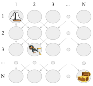
(a) Deep Sea

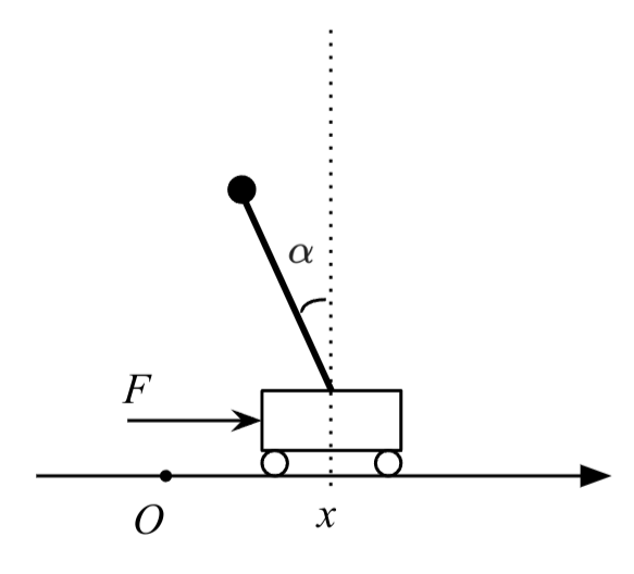
(b) Cartpole Swingup

Figure 1: bsuite environments

Deep Sea

The environment is an $N\times N$ grid with one-hot state encoding. The agent starts from the top left corner of the grid and descends down-left or down-right in each timestep, depending on the action. There is a small cost of $r=-0.01/N$ for moving right, and $r=0$ for moving left. If the agent reaches the bottom-right corner, taking only “right” actions, it gets a reward of $+1$. This is a simple but challenging exploration problem, due to the fact that exploring uniformly at random only has a $2^{-N}$ chance of finding the high-reward state.

Cartpole Swingup

The goal is to swing up and balance an unactuated pole by applying forces to a cart at its base. The physics model conforms to Barto et al. (1983). The pole starts from a random position pointing down, and the agent can apply a force of $-1$, $0$, or $1$ to the cart. There is a small cost of $r=-0.1$ for applying a non-zero force. The agent gets a reward of $+1$ if the pole is within a small angle of being upright and the cart is within a small range around the origin. We consider two versions of this environment: default and hard versions, where the hard version has sparser rewards. More details on how the rewards are defined in the two versions can be found in Appendix C.2.

Our experiments for bsuite environments involve four agents: BootDDQN, DDQN-Bonus, vanilla DDQN, and PI-Bonus. For BootDDQN, we use standard deviation of the ensemble as the uncertainty metric $u_{\text{std}}$. For all other agents, we use the covariance-based uncertainty $u_{\text{cov}}$. The confidence intervals are calculated with $10$ random seeds for Deep Sea and $20$ seeds for Cartpole Swingup. DDQN-Intrinsic does not converge in our Deep Sea and Cartpole Swingup experiments due to numerical issues. Therefore, we do not report the results of DDQN-Intrinsic in this section.

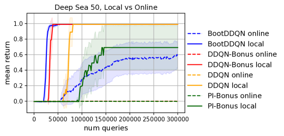
Figure 2: Local and online access on Deep Sea 50. Curves with the same color correspond to the same agent. Dashed and solid curves correspond to online and local access, respectively.

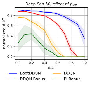
(a) The effect of $p_{\text{init}}$

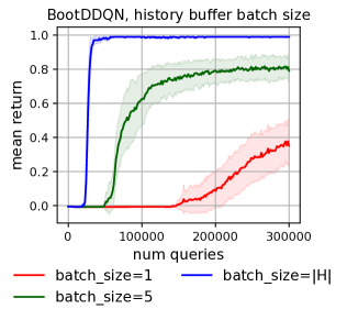
(b) The effect of $B$

Figure 3: The effect of $p_{\text{init}}$ and history buffer batch size $B$ in Deep Sea 50. Choosing $B=1$ is equivalent to choosing a random element in the history buffer, without considering uncertainty.

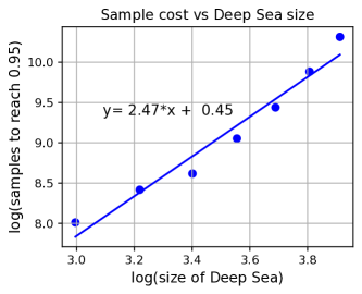
Figure 4: The number of queries needed to achieve mean return $0.95$ vs the size of the Deep Sea environment (BootDDQN).

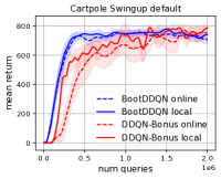
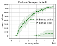
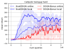
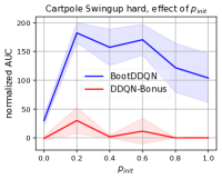
Figure 5: Cartpole Swingup results. (a) BootDDQN and DDQN-Bonus in the default version. (b) PI-Bonus in the default version. (c) BootDDQN and DDQN-Bonus in the hard version. (d) The effect of $p_{\text{init}}$ in the hard version for BootDDQN and DDQN-Bonus.

Deep Sea results

We first compare the return of the agents on Deep Sea with size $N=50$ in the online and local access (UFLP) settings. We use $p_{\text{init}}=0.1$ and history buffer batch size $B=|\mathcal{H}|$ (i.e., we choose the most uncertain state-action pair from the entire history buffer) for all the local access runs. As we can see from Figure 2, local access leads to significantly higher mean return for each agent. In fact, in the online setting, except for BootDDQN, none of the agents can get a return that is significantly higher than $0$ within $3\times 10^{5}$ simulator queries. Therefore, in this hard-exploration environment, local access significantly improves the sample efficiency.

We also investigate the role of $p_{\text{init}}$ and history buffer batch size $B$ in Deep Sea. In Figure 3(a), we plot the normalized area under curve (AUC) for the the convergence curves in Figure 2 as a function of $p_{\text{init}}$. This quantity reflects how fast the return converges. The best performance is achieved with a relatively small $p_{\text{init}}$ (e.g., $0.0\sim 0.3$) for most agents. This demonstrates the benefits of data collection from intermediate states. In Figure 3, we compare the sample efficiency of BootDDQN with $B=1,5,$ and $|\mathcal{H}|$. As we can see, the best performance is achieved with $B=|\mathcal{H}|$, i.e., choosing the most uncertain element in the history buffer. This demonstrates the importance of starting from an uncertain state in Deep Sea. In Appendix A.1, we provide similar results for other agents.

In Figure 4, we show the number of queries needed to achieve mean return $0.95$, for the BootDDQN agent, as a function of the size of the Deep Sea environment $N$, to illustrate the scaling of the sample cost. Our results indicates a near-optimal dependency of $\mathcal{O}(N^{2.47})$.

Cartpole Swingup results

For the default version of Cartpole Swingup, we find that for BootDDQN and DDQN-Bonus agents, the sample efficiency of online and local access modes are similar (Figure 5(a)), whereas for the PI-Bonus agent, local access leads to a significant improvement (Figure 5(b)). This indicates that for environments with relatively dense reward, the benefit of local access can be small, especially for value-based agents. For the hard version, for both BootDDQN and DDQN-Bonus agents, we find that local access leads to a significant improvement over online access (Figure 5(c)). We did not observe positive rewards in the hard version of Cartpole Swingup using the PI-Bonus agent, regardless of the access protocol. In Figure 5(d), we show that the best performance can be achieved with a relatively small $p_{\text{init}}$, e.g., $0.2$, for the hard version of Cartpole Swingup. One observation is that when $p_{\text{init}}=0.0$, the performance is bad. We hypothesize that this is because for $p_{\text{init}}=0.0$, we only observe a single initial state from the initial-state distribution, and the agent may not have enough information on how to act from other initial states.

6.2 Atari

In this section, we evaluate our approach on four Atari games from the Arcade Learning Environment (ALE) (Bellemare et al., 2013):

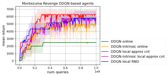
Figure 6: Uncertainty-first local planning vs. online access on Montezuma’s Revenge with DDQN-based agents.

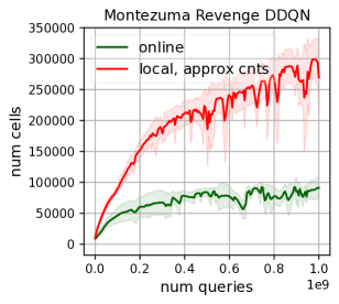
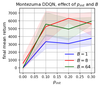
Figure 7: (a) The number of cells found by the DDQN agent in the online and local settings using the approximate-count-based uncertainty. (b) The effect of $p_{\text{init}}$ and history buffer batch size $B$. Again we note that choosing $B=1$ is equivalent to choosing a random element in the history buffer, without considering uncertainty.

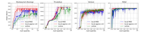
Figure 8: Uncertainty-first local planning vs. online access on hard-exploration Atari games with a distributional DDQN agent.

Montezuma’s Revenge

Montezuma’s Revenge (MR) has sparser rewards than most ALE environments. The agent only receives positive rewards after performing a long series of specific actions. MR has been viewed as one of the most difficult exploration challenges for deep RL. A few approaches surpassing average human performance of 4753 points (Badia et al., 2020a) include RND (Burda et al., 2018), NGU (Badia et al., 2020b), Agent57 (Badia et al., 2020a), and MEME (Kapturowski et al., 2022). The SOTA of 43K is achieved by Go-Explore (Ecoffet et al., 2021).

Pitfall

This is another highly challenging exploration game in ALE. In addition to sparse positive rewards, Pitfall includes distractor rewards, such as small negative rewards for hitting an enemy, and is only partially observable. Most agents obtain zero reward, and a few exceptions include NGU, Agent57, MEME, and Go-Explore.

PrivateEye

This is also a sparse reward game. The average human performance is 69K (Badia et al., 2020a).

Venture

Rewards are denser than in the $3$ other games, and the average human score is 1187 (Badia et al., 2020a).

As base agents, we use the DDQN and distributional DDQN implementations in the Acme framework (Hoffman et al., 2020) for distributed RL. In Acme, agent functionality is split into multiple actors, which collect data and write to the replay buffer, and a single learner which updates the agent parameters based on replay data. In our implementation, the actors also write to a common (smaller) history buffer, and choose states to reset to from the history buffer based on uncertainty. We experiment with two different uncertainty metrics: approximate counts and RND. For approximate counts, we downsample the grayscale game images to a shape of $(12,12)$, and discretize the pixel values to $8$ levels. For RND, the random features are extracted by the Q-network architecture followed by a 2-layer MLP with embedding size $1024$. The predictor also has the same architecture. More implementation details and hyperparameters are given in Appendix C.3. All the confidence intervals in this section are calculated using $5$ random seeds.

We first evaluate agents on Montezuma’s Revenge. For the online setting, we use the vanilla DDQN and DDQN-Intrinsic agents, with the intrinsic reward based on approximate-count uncertainty. For the local setting, we combine DDQN with both approximate-count and RND based uncertainty. We also experiment with DDQN-Intrinsic in the local setting with approximate counts.

Figure 6 shows that local access significantly improves the final return over online access for both uncertainty metrics. Here, we emphasize that reaching a higher final return using the same number of simulator queries implies that an algorithm has better sample efficiency. In Figure 7(a), we plot the number of cells (when using approximate counts) found by the online and local DDQN agents. As expected, in the local access setting, the agent finds more cells, indicating that a larger state space is discovered. Similar results for DDQN-Intrinsic can be found in Appendix A.3. In Figure 7(b), we study the role of $p_{\text{init}}$ and history buffer batch size $B$ in DDQN with approximate counts. We can see that $B=8,64$ is significantly better than $B=1$, indicating the importance of starting from an uncertain state. We also observe that $p_{\text{init}}=0.0$ is a bad choice in this game. We hypothesize that this is due to the fact that in our implementation, the actors only maintain the approximate counts of the cells that they have visited, rather than cells that exist in the replay buffer. Thus, when $p_{\text{init}}=0.0$, there are not enough data in the replay buffer that correspond to the state space near the initial state, and as the result the agent forgets how to act at the beginning of the episode. However, choosing $p_{\text{init}}\in[0.1,0.3]$ leads to similar performance.

We also observe improvement for the DDQN-Intrinsic agent using local access (Figure 6). However, since DDQN-Intrinsic already has an exploration bonus in the intrinsic reward, the additional benefit of local planning is relatively small. We note that for DDQN-Intrinsic, to get good performance in the local setting, we need to choose a larger value of $p_{\text{init}}$, i.e., $0.7$. This means that we need to reduce the amount of local access iterations in order to reach a good balance between exploration and exploitation.

We evaluate the performance of distributional DDQN with UFLP ($p_{\text{init}}=0.3$) for both approximate-count and RND uncertainty on all four Atari games. As we can see in Figure 8, on Montezuma’s Revenge, local planning dramatically improves the score of the baseline algorithm to a super-human level. On PrivateEye, local access improves the sample complexity and stability of the baseline algorithm. Venture results are neutral, possibly because the rewards are relatively dense and thus the exploration problem is less challenging compared to other games. On Pitfall, both local and and online access versions fail to obtain positive scores. We conjecture that this is due to the partially-observable nature of this MDP; indeed, prior works that have obtained positive scores have relied on side information, stateful policies, or both (Badia et al., 2020a; Ecoffet et al., 2019, 2021).

We summarize all Atari results in Appendix A.3 and include the highest scores obtained by actors during data collection. Note that actor returns are sometimes considerably higher than those of the learned policy (greedy w.r.t. the Q-function), e.g. $14300$ vs. $7100$ for Montezuma’s Revenge and $1800$ vs. $0$ for Pitfall. This suggests the performance of the DDQN agents could be improved by more effective learning (not addressed here) in addition to exploration.

7 Conclusions and Future Directions

We propose a new algorithmic framework for learning with a simulator under the local access protocol. We demonstrate that our proposed uncertainty-first approach to revisiting states in history can dramatically improve the sample cost of several baseline algorithms on sparse-reward environments. An important direction for future work is improving the quality of uncertainty estimation in MDPs, since the this directly affects the effectiveness of the framework. Another interesting direction for future work is to extend this approach to partially observed environments.

Appendix A Additional Experimental Results

A.1 Deep Sea

In Figure 9, we show the effect of history buffer batch size $B$ for the DDQN-Bonus, DDQN, and PI-Bonus agents in Deep Sea 50. As we can see, the best performance is achieved with $B=|\mathcal{H}|$. Therefore, it is important to start the data collection process with an uncertain state.

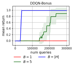
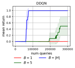
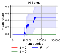
Figure 9: The effect of history buffer batch size $B$ for the DDQN-Bonus, DDQN, and PI-Bonus agents in Deep Sea 50.

A.2 Cartpole Swingup

We provide additional results on the Cartpole Swingup environment. In Figure 10(a), we fix the history buffer batch size $B=5$ and study the effect of $p_{\text{init}}$ in the default version. We observe that $p_{\text{init}}=0.0$ is a bad choice, as discussed in Section 6.1. We also observe that for BootDDQN and DDQN-Bonus, the performance is comparable for $p_{\text{init}}$ values in $[0.2,1.0]$. This is due to the fact that in the reward is not very sparse in this version and thus local access does not lead to significant improvement. On the other hand, for PI-Bonus, local access leads to significant improvement over online access, and the best performance is achieved with a relatively small but non-zero $p_{\text{init}}$, i.e., $0.2$. In Figure 10(b), we fix $p_{\text{init}}=0.2$ and study the effect of the history buffer batch size $B$ for the default version of the environment. Again for BootDDQN and DDQN-Bonus, since local access does not lead to significant improvement, the performance is comparable for different values of $B$. But for PI-Bonus, choosing an uncertain element, i.e., $B>1$ is important. In Figure 10(c), we fix $p_{\text{init}}=0.2$ and study the effect of the history buffer batch size $B$ for the hard version of the environment. Interestingly, we found that for BootDDQN, the normalized AUCs for $B=1,5,25,125$ are comparable. Note that when $B=1$, we ignore the uncertainty and simply choose a random element from the history buffer. This indicates that for BootDDQN in the hard version of Cartpole Swingup, the gain of local access mainly comes from directly starting from an intermediate state, i.e., skipping the simulator queries from the initial state to the chosen one, and the uncertainty is less important for this setting.

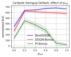
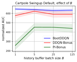
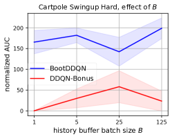
Figure 10: (a) The effect of $p_{\text{init}}$ in the default version of Cartpole Swingup. (b) The effect of history buffer batch size $B$ in the default version of Cartpole Swingup. (c) The effect of history buffer batch size $B$ in the hard version of Cartpole Swingup.

A.3 Atari

In Figure 11, we show the number of cells found by the DDQN-Intrinsic agent in the online and local settings. As we can see, with local access, the agent finds more cells than the online setting. This indicates that using local access, the agent can find a larger state space. On the other hand, comparing Figure 11 and Figure 7(a), we notice that using DDQN-Intrinsic and online access, we can find more cells than using DDQN and local access. However, DDQN with local access achieves better mean return. This implies that finding more cells created by the approximate-count based method does not necessarily lead to a better mean return.

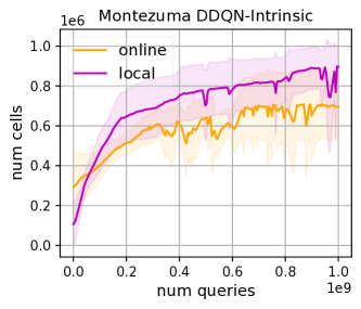
Figure 11: The number of cells found by the DDQN-Intrinsic agent in the online and local settings.

Table 1: Evaluation results of DDQN-based agents on Montezuma’s Revenge

Agent and access protocol	Result
DDQN online	2500.0 $\pm$ 0.0
DDQN-Intrinsic online	4980.0 $\pm$ 1086.91
DDQN-Intrinsic local	5518.0 $\pm$ 491.6
DDQN local, approx count	6276.0 $\pm$ 551.3
DDQN local, RND	5772.0 $\pm$ 955.75

Table 2: Evaluation results, distributional DDQN

Game	Online	Local approx count	Local RND
Montezuma’s Revenge	4421.33 $\pm$ 869.63	6235.33 $\pm$ 860.91	5534.0 $\pm$ 118.11
PrivateEye	88258.27 $\pm$ 15908.99	100645.17 $\pm$ 62.16	100571.25 $\pm$ 93.18
Venture	1792.67 $\pm$ 37.39	1803.33 $\pm$ 50.34	1691.33 $\pm$ 33.4
Pitfall	-1.31 $\pm$ 0.91	0.0 $\pm$ 0.0	-2.21 $\pm$ 2.29

We report the evaluation results of the DDQN-based agents in Table 1 and distributional DDQN in Table 2. For each seed, we consider the final performance of the agent to be the average of its last 30 evaluation runs. We then average this over 5 seeds and report this with 95% confidence intervals. The number of environment steps is $10^{9}$ for Montezuma’s revenge, and $2\times 10^{8}$ for the other Atari environments. We also report the maximum screen score that was seen during the acting over all seeds in Tables 3 and 4. We calculate this by considering the screen score of a state as the sum of unclipped rewards attained till that state. Note that this score need not have been attained in a single data collection iteration in the local access setting. The agent could reset to a intermediate state with positive screen score, and then obtain the maximum screen achieved so far after several further steps.

On Montezuma’s Revenge, the distributional DDQN local agent with approximate count uncertainty reaches a screen score $14300$. We note that we also observe screen scores $>100000$ on this environment, but believe this may be due to triggering a treasure room curse bug, also mentioned in Ecoffet et al. (2019). We also note that at least one of the RND local planning agent seeds reach a positive screen score on Pitfall.

Table 3: Maximum screen score during data collection, DDQN-based agents on Montezuma’s Revenge

Agent and access protocol	Result
DDQN online	3000
DDQN-Intrinsic online	6600
DDQN-Intrinsic local	8900
DDQN local, approx count	9500
DDQN local, RND	8000

Table 4: Maximum screen score during data collection, distributional DDQN

Game	Online	Local approx count	Local RND
Montezuma’s Revenge	6000	14300	6500
PrivateEye	100800	100800	100800
Venture	2200	3000	2600
Pitfall	0	0	1800

Appendix B Checkpointing and Restoring the Environment

For bsuite environments, since the simulators are implemented in Python, we can use the deep copy function to checkpoint and restore the environment state.

⬇

import copy

def make_env_checkpoint(env):

return copy.deepcopy(env)

def restore_env(env_copy):

return copy.deepcopy(env_copy)

For Atari games, we use the environment loader in the open-sourced Acme framework. We use the “clone” and “restore” function of the environment to make checkpoints and restore the states. Note that since we stack the last 4 frames of the game, we also need to checkpoint and restore the frame stack.

⬇

import collections

import copy

import numpy as np

def make_env_checkpoint(env):

state=env.unwrapped.clone_full_state()

stacker_state=copy.deepcopy(np.array(env._frame_stacker._stack))

stacker_max_size=env._frame_stacker._stack.maxlen

return state, stacker_state, stacker_max_size

def restore_env(env, state, stacker_state, stacker_max_size):

env.unwrapped.restore_full_state(element.state)

env._environment._frame_stacker._stack = collections.deque(

copy.deepcopy(element.stacker_state),

maxlen=element.stacker_max_size)

return env

Appendix C Hyperparameters

C.1 Deep Sea

For all the Q-networks used in our experiments on Deep Sea, we use an MLP with two hidden layers, each with size $64$.

For the BootDDQN agent, we use an ensemble of size $20$ and a prior scale (Osband et al., 2018) of $40.0$. For all other agents, we use covariance-based uncertainty metric $u_{\text{cov}}$ with random Fourier features. We choose feature dimension $d=1500$. For DDQN and DDQN-Bonus, we choose regularization coefficient $\lambda=0.01$ and for PI-Bonus, we choose $\lambda=0.1$. For DDQN-Bonus and PI-Bonus, we use bonus scale $c=1.0$. In all the experiments, we use a replay buffer of size $10^{6}$, sufficient to store all the transitions in the experiments. All other hyperparameter are provided in Table 5. In the table, SGD period means the number of new observations we obtain before starting a new SGD training step; environment checkpoint period means the number of observations we obtain before saving a new environment checkpoint in the history buffer.

Table 5: Hyperparameters for Deep Sea experiments

Hyperparameter	Value
discount $\gamma$	$1.0$ for PI-Bonus, $0.99$ for other agents
$\epsilon$-greedy	$0.1$ for DDQN-Bonus, $0.0$ for other agents
SGD period	$4$ for PI-Bonus, $1$ for all other agents
target update period	$4$ (N/A for PI-Bonus)
environment checkpoint period	$1$
learning batch size	$128$
optimizer	Adam
learning rate	$0.001$
maximum gradient norm for clipping	$20$

C.2 Cartpole Swingup

Environment parameters

Recall that in Figure 1, the horizontal position of the cart is denoted by $x$, the angle between the pole and the upright direction is denoted by $\alpha$. We also denote the angular velocity of the pole by $\dot{\alpha}$. In the default version, the agent receives a positive reward if the following conditions are satisfied:

$$\begin{cases}&|x|<1.0\\ &\cos\alpha>0.5\\ &|\dot{\alpha}|<1.0,\end{cases}$$

and in the hard version, the agent receives a positive reward if the following conditions are satisfied:

$$\begin{cases}&|x|<0.05\\ &\cos\alpha>0.95\\ &|\dot{\alpha}|<1.0.\end{cases}$$

Therefore, the reward is more sparse in the hard version.

Agent hyperparameters

For all the Q-networks used in our experiments on Cartpole Swingup, we use an MLP with two hidden layers, each with size $128$.

For BootDDQN, we sweep different combinations of ensemble size and prior scale to determine the best combination and then use it in the local setting. For the default version, we use an ensemble of size $5$ and prior scale of $5.0$. For the hard version, we use an ensemble of size $10$ and prior scale of $5.0$. We use $\epsilon=0.2$ for BootDDQN.

For DDQN-Bonus and PI-Bonus, we use random Fourier feature of dimension $d=500$ and regularization coefficient $\lambda=0.1$. For DDQN-Bonus, we sweep the bonus scale parameter $c$ and the $\epsilon$-greedy parameter in the online setting and use the best combination in the local setting. For DDQN-Bonus, in the default version of Cartpole Swingup, we use bonus scale $c=10$ and $\epsilon=0.2$, and in the hard version of Cartpole Swingup, we use bonus scale $c=100$ and $\epsilon=0.0$. For PI-Bonus, we use bonus scale $c=500$ and $\epsilon=0.0$.

As for the hyperparameters for local planning, we use a history buffer of size $10^{5}$. We sweep different combinations of $p_{\text{init}}$ and history buffer batch size $B$ and choose the best combination for each agent. The hyperparameters that we choose for results in Figure 5(a, b, c) are given in Table 6.

Table 6: Local planning hyperparameters in Figure 5.

Agent	Version	$p_{\text{init}}$	$B$
BootDDQN	default	$0.8$	$5$
DDQN-Bonus	default	$0.2$	$5$
PI-Bonus	default	$0.2$	$5$
BootDDQN	hard	$0.4$	$125$
DDQN-Bonus	hard	$0.2$	$25$

All other hyperparameters are provided in Table 7.

Table 7: Hyperparameters for Cartpole Swingup experiments

Hyperparameter	Value
discount $\gamma$	$0.99$ for BootDDQN and DDQN-Bonus, $0.995$ for PI-Bonus
SGD period	$25$ for BootDDQN and DDQN-Bonus, $5$ for PI-Bonus
target update period	$10$ (N/A for PI-Bonus)
environment checkpoint period	$5$
learning batch size	$2048$ for BootDDQN and DDQN-Bonus, $256$ for PI-Bonus
optimizer	Adam
learning rate	$0.001$
maximum gradient norm for clipping	$20$

C.3 Atari

Environment parameters

We run experiments on the v0 version of Atari environments with sticky actions, making the environments stochastic (Machado et al., 2018). We apply the standard frame processing wrapper provided in Acme, which includes converting the frames to grayscale, downsampling, stacking $4$ consecutive frames for each observation. We summarize the environment hyperparameters in Table 8.

Table 8: Hyperparameters for Atari environments.

Hyperparameter	Value
max episode length	$30$ min ($108,000$ steps)
number of stacked frames	$4$
zero discount on life loss	false
random noops range $30$	not used
sticky actions	true, repeat action probability $0.25$
frame size	$(84,84)$
grayscaled/RGB	grayscaled
action set	full

Agent hyperparameters

As for model architecture, for both DDQN-based agents and distributional DDQN, we use the Acme AtariTorso network architecture followed by an MLP with 512 hidden units.

As for local planning hyperparameters, we use a history buffer of size $10^{6}$. Under local access, we reset to the highest-uncertainty state in the sampled batch, and then take a random action, i.e., Eq. equation 2. For the DDQN-based agents in Figure 6, for local access runs, we sweep different combinations of $p_{\text{init}}$ and $B$ and report the results corresponding to the best combination we can find. The values of $p_{\text{init}}$ and $B$ that we use in the experiments in Figure 6 are provided in Table 9. For the DDQN agent in Montezuma’s Revenge, we find that using $\epsilon=0.1$ leads to better results in the online setting, and thus we choose $\epsilon=0.1$ for this setting. We use $\epsilon=0.01$ for all other settings. For the distributional DDQN agent, the local access runs in Figure 8, we use $p_{\text{init}}=0.3$ and history buffer batch size $B=32$.

Table 9: Local planning hyperparameters in Figure 6.

Agent	$p_{\text{init}}$	$B$
DDQN local approximate count	$0.2$	$8$
DDQN-Intrinsic local approximate count	$0.7$	$8$
DDQN local RND	$0.3$	$32$

In Montezuma’s Revenge, in order to limit online access queries which do not lead to significant exploration, and also have more exploration around uncertain regions, we limit the maximum length of all roll-outs to $2000$. Another possible benefit of this is the composition of the limited size replay buffer is more uniform, and not dominated by certain long rollouts from unimportant regions. For all other settings, including both online and local access for other games, and the online access setting for Montezuma’s Revenge, we did not find this option helpful. Thus, we run rollout until the end of the episode for all other settings.

The remaining hyperparameters corresponding to the Acme DDQN config are given in Table 10. Compared to the default settings, we do not use prioritized replay sampling, we clip gradients, and we use higher “samples per insert”, which governs the average number of times a transition is sampled by the learner before being evicted from the replay buffer. We did not find prioritized sampling to help the performance of either the online or local access agent on Montezuma’s Revenge. For the training system, we use $64$ CPU machines as actors and $1$ TPU machine as the learner in most settings. The only exception is that for RND we use $128$ actors in order to speedup training. We did not find using $128$ actors improving the online baseline.

Table 10: Hyperparameter values for experiments on Atari games.

Hyperparameter	Value
discount $\gamma$	$0.997$ for PrivateEye, $0.99$ for all other games
learning batch size	$256$ for distributional DDQN, $128$ for DDQN and DDQN-Intrinsic
learning rate	$10^{-4}$ for DDQN and DDQN-Intrinsic
	chosen between $10^{-4}$ and $2\times 10^{-5}$ for distributional DDQN
epsilon	$0.1$ for DDQN online in Montezuma’s Revenge, $0.01$ otherwise
eval epsilon	$0$
Adam epsilon	$10^{-5}$
number of TD steps (n_step)	$5$ for distributional DDQN, $3$ for DDQN and DDQN-Intrinsic
target update period	$2500$
environment checkpointing period	$10$
number of actors	$128$ for experiments with RND, $64$ otherwise
max gradient norm	$10$
min replay size	$5\times 10^{4}$
max replay size	$5\times 10^{6}$
importance sampling exponent	$0$
priority exponent	$0$
samples per insert	$8$
number of SGD steps per step	$8$
number of atoms in distributional DDQN	$201$
$v_{\min}$ in distributional DDQN	$-1$
$v_{\max}$ in distributional DDQN	$120000$ for PrivateEye, $20000$ for all other games
$v_{\max}$ in distributional DDQN RND	$120000$ for PrivateEye, $10000$ for all other games
bonus scale $c$ in DDQN-Intrinsic	$0.1$
reward clipping	$1$ for DDQN and DDQN-Intrinsic, N/A for distribution DDQN

References

- Agarwal et al. (2020) A. Agarwal, M. Henaff, S. Kakade, and W. Sun. PC-PG: Policy cover directed exploration for provable policy gradient learning. arXiv preprint arXiv:2007.08459, 2020.
- Akkaya et al. (2019) I. Akkaya, M. Andrychowicz, M. Chociej, M. Litwin, B. McGrew, A. Petron, A. Paino, M. Plappert, G. Powell, R. Ribas, et al. Solving rubik’s cube with a robot hand. arXiv preprint arXiv:1910.07113, 2019.
- Aradi (2020) S. Aradi. Survey of deep reinforcement learning for motion planning of autonomous vehicles. IEEE Transactions on Intelligent Transportation Systems, 2020.
- Badia et al. (2020a) A. P. Badia, B. Piot, S. Kapturowski, P. Sprechmann, A. Vitvitskyi, Z. D. Guo, and C. Blundell. Agent57: Outperforming the atari human benchmark. In International Conference on Machine Learning, pages 507–517. PMLR, 2020a.
- Badia et al. (2020b) A. P. Badia, P. Sprechmann, A. Vitvitskyi, D. Guo, B. Piot, S. Kapturowski, O. Tieleman, M. Arjovsky, A. Pritzel, A. Bolt, et al. Never give up: Learning directed exploration strategies. arXiv preprint arXiv:2002.06038, 2020b.
- Barto et al. (1983) A. G. Barto, R. S. Sutton, and C. W. Anderson. Neuronlike adaptive elements that can solve difficult learning control problems. IEEE Transactions on Systems, Man, and Cybernetics, 13(5):834–846, 1983.
- Barto et al. (1995) A. G. Barto, S. J. Bradtke, and S. P. Singh. Learning to act using real-time dynamic programming. Artificial Intelligence, 72(1-2):81–138, 1995.
- Beattie et al. (2016) C. Beattie, J. Z. Leibo, D. Teplyashin, T. Ward, M. Wainwright, H. Küttler, A. Lefrancq, S. Green, V. Valdés, A. Sadik, et al. DeepMind Lab. arXiv preprint arXiv:1612.03801, 2016.
- Bellemare et al. (2016) M. Bellemare, S. Srinivasan, G. Ostrovski, T. Schaul, D. Saxton, and R. Munos. Unifying count-based exploration and intrinsic motivation. Advances in Neural Information Processing Systems, 29, 2016.
- Bellemare et al. (2013) M. G. Bellemare, Y. Naddaf, J. Veness, and M. Bowling. The arcade learning environment: An evaluation platform for general agents. Journal of Artificial Intelligence Research, 47:253–279, 2013.
- Bellemare et al. (2017) M. G. Bellemare, W. Dabney, and R. Munos. A distributional perspective on reinforcement learning. In International Conference on Machine Learning, pages 449–458. PMLR, 2017.
- Bertsekas (2011) D. P. Bertsekas. Approximate policy iteration: A survey and some new methods. Journal of Control Theory and Applications, 9(3):310–335, 2011.
- Bojarski et al. (2016) M. Bojarski, D. Del Testa, D. Dworakowski, B. Firner, B. Flepp, P. Goyal, L. D. Jackel, M. Monfort, U. Muller, J. Zhang, et al. End to end learning for self-driving cars. arXiv preprint arXiv:1604.07316, 2016.
- Brockman et al. (2016) G. Brockman, V. Cheung, L. Pettersson, J. Schneider, J. Schulman, J. Tang, and W. Zaremba. OpenAI Gym. arXiv preprint arXiv:1606.01540, 2016.
- Burda et al. (2018) Y. Burda, H. Edwards, A. Storkey, and O. Klimov. Exploration by random network distillation. arXiv preprint arXiv:1810.12894, 2018.
- Chen et al. (2017) R. Y. Chen, S. Sidor, P. Abbeel, and J. Schulman. UCB exploration via Q-ensembles. arXiv preprint arXiv:1706.01502, 2017.
- Coulom (2006) R. Coulom. Efficient selectivity and backup operators in Monte-Carlo tree search. In International Conference on Computers and Games, pages 72–83. Springer, 2006.
- Degrave et al. (2022) J. Degrave, F. Felici, J. Buchli, M. Neunert, B. Tracey, F. Carpanese, T. Ewalds, R. Hafner, A. Abdolmaleki, D. de Las Casas, et al. Magnetic control of tokamak plasmas through deep reinforcement learning. Nature, 602(7897):414–419, 2022.
- Du et al. (2020) S. S. Du, S. M. Kakade, R. Wang, and L. F. Yang. Is a good representation sufficient for sample efficient reinforcement learning? In International Conference on Learning Representations, 2020.
- Ecoffet et al. (2019) A. Ecoffet, J. Huizinga, J. Lehman, K. O. Stanley, and J. Clune. Go-explore: a new approach for hard-exploration problems. arXiv preprint arXiv:1901.10995, 2019.
- Ecoffet et al. (2021) A. Ecoffet, J. Huizinga, J. Lehman, K. O. Stanley, and J. Clune. First return, then explore. Nature, 590(7847):580–586, 2021.
- Hao et al. (2022) B. Hao, N. Lazić, D. Yin, Y. Abbasi-Yadkori, and C. Szepesvári. Confident least square value iteration with local access to a simulator. The 25th International Conference on Artificial Intelligence and Statistics, 2022.
- Hoffman et al. (2020) M. W. Hoffman, B. Shahriari, J. Aslanides, G. Barth-Maron, N. Momchev, D. Sinopalnikov, P. Stańczyk, S. Ramos, A. Raichuk, D. Vincent, L. Hussenot, R. Dadashi, G. Dulac-Arnold, M. Orsini, A. Jacq, J. Ferret, N. Vieillard, S. K. S. Ghasemipour, S. Girgin, O. Pietquin, F. Behbahani, T. Norman, A. Abdolmaleki, A. Cassirer, F. Yang, K. Baumli, S. Henderson, A. Friesen, R. Haroun, A. Novikov, S. G. Colmenarejo, S. Cabi, C. Gulcehre, T. L. Paine, S. Srinivasan, A. Cowie, Z. Wang, B. Piot, and N. de Freitas. Acme: A research framework for distributed reinforcement learning. arXiv preprint arXiv:2006.00979, 2020.
- Jin et al. (2020) C. Jin, Z. Yang, Z. Wang, and M. I. Jordan. Provably efficient reinforcement learning with linear function approximation. In Conference on Learning Theory, pages 2137–2143. PMLR, 2020.
- Kakade (2003) S. M. Kakade. On the sample complexity of reinforcement learning. University of London, University College London (United Kingdom), 2003.
- Kapturowski et al. (2022) S. Kapturowski, V. Campos, R. Jiang, N. Rakićević, H. van Hasselt, C. Blundell, and A. P. Badia. Human-level Atari 200x faster. arXiv preprint arXiv:2209.07550, 2022.
- Kocsis and Szepesvári (2006) L. Kocsis and C. Szepesvári. Bandit based Monte-Carlo planning. In Machine Learning: ECML 2006: 17th European Conference on Machine Learning Berlin, Germany, September 18-22, 2006 Proceedings 17, pages 282–293. Springer, 2006.
- Lan et al. (2023) L.-C. Lan, H. Zhang, and C.-J. Hsieh. Can agents run relay race with strangers? generalization of RL to out-of-distribution trajectories. arXiv preprint arXiv:2304.13424, 2023.
- Lazic et al. (2021) N. Lazic, D. Yin, Y. Abbasi-Yadkori, and C. Szepesvari. Improved regret bound and experience replay in regularized policy iteration. arXiv preprint arXiv:2102.12611, 2021.
- Li et al. (2021) G. Li, Y. Chen, Y. Chi, Y. Gu, and Y. Wei. Sample-efficient reinforcement learning is feasible for linearly realizable MDPs with limited revisiting. arXiv preprint arXiv:2105.08024, 2021.
- Machado et al. (2018) M. C. Machado, M. G. Bellemare, E. Talvitie, J. Veness, M. Hausknecht, and M. Bowling. Revisiting the arcade learning environment: Evaluation protocols and open problems for general agents. Journal of Artificial Intelligence Research, 61:523–562, 2018.
- McMahan et al. (2005) H. B. McMahan, M. Likhachev, and G. J. Gordon. Bounded real-time dynamic programming: RTDP with monotone upper bounds and performance guarantees. In Proceedings of the 22nd International Conference on Machine Learning, pages 569–576, 2005.
- Mnih et al. (2015) V. Mnih, K. Kavukcuoglu, D. Silver, A. A. Rusu, J. Veness, M. G. Bellemare, A. Graves, M. Riedmiller, A. K. Fidjeland, G. Ostrovski, et al. Human-level control through deep reinforcement learning. Nature, 518(7540):529–533, 2015.
- Osband et al. (2016) I. Osband, C. Blundell, A. Pritzel, and B. Van Roy. Deep exploration via bootstrapped DQN. Advances in Neural Information Processing Systems, 29, 2016.
- Osband et al. (2018) I. Osband, J. Aslanides, and A. Cassirer. Randomized prior functions for deep reinforcement learning. Advances in Neural Information Processing Systems, 31, 2018.
- Osband et al. (2019) I. Osband, Y. Doron, M. Hessel, J. Aslanides, E. Sezener, A. Saraiva, K. McKinney, T. Lattimore, C. Szepesvari, S. Singh, et al. Behaviour suite for reinforcement learning. arXiv preprint arXiv:1908.03568, 2019.
- Pathak et al. (2017) D. Pathak, P. Agrawal, A. A. Efros, and T. Darrell. Curiosity-driven exploration by self-supervised prediction. In International Conference on Machine Learning, pages 2778–2787. PMLR, 2017.
- Qassem et al. (2010) M. A. Qassem, I. Abuhadrous, and H. Elaydi. Modeling and simulation of 5 dof educational robot arm. In 2010 2nd International Conference on Advanced Computer Control, volume 5, pages 569–574. IEEE, 2010.
- Rahimi and Recht (2007) A. Rahimi and B. Recht. Random features for large-scale kernel machines. Advances in Neural Information Processing Systems, 20, 2007.
- Salimans and Chen (2018) T. Salimans and R. Chen. Learning montezuma’s revenge from a single demonstration. arXiv preprint arXiv:1812.03381, 2018.
- Sanner et al. (2009) S. Sanner, R. Goetschalckx, K. Driessens, and G. Shani. Bayesian real-time dynamic programming. In Proceedings of the 21st International Joint Conference on Artificial Intelligence (IJCAI-09), pages 1784–1789. IJCAI-INT JOINT CONF ARTIF INTELL, 2009.
- Schulman et al. (2015) J. Schulman, S. Levine, P. Abbeel, M. Jordan, and P. Moritz. Trust region policy optimization. In International Conference on Machine Learning, pages 1889–1897. PMLR, 2015.
- Schulman et al. (2017) J. Schulman, F. Wolski, P. Dhariwal, A. Radford, and O. Klimov. Proximal policy optimization algorithms. arXiv preprint arXiv:1707.06347, 2017.
- Sherman and Morrison (1950) J. Sherman and W. J. Morrison. Adjustment of an inverse matrix corresponding to a change in one element of a given matrix. The Annals of Mathematical Statistics, 21(1):124–127, 1950.
- Sidford et al. (2018) A. Sidford, M. Wang, X. Wu, L. Yang, and Y. Ye. Near-optimal time and sample complexities for solving Markov decision processes with a generative model. In Proceedings of the 32nd International Conference on Neural Information Processing Systems, pages 5192–5202, 2018.
- Silver et al. (2016) D. Silver, A. Huang, C. J. Maddison, A. Guez, L. Sifre, G. Van Den Driessche, J. Schrittwieser, I. Antonoglou, V. Panneershelvam, M. Lanctot, et al. Mastering the game of go with deep neural networks and tree search. Nature, 529(7587):484–489, 2016.
- Silver et al. (2018) D. Silver, T. Hubert, J. Schrittwieser, I. Antonoglou, M. Lai, A. Guez, M. Lanctot, L. Sifre, D. Kumaran, T. Graepel, et al. A general reinforcement learning algorithm that masters chess, shogi, and go through self-play. Science, 362(6419):1140–1144, 2018.
- Smith and Simmons (2006) T. Smith and R. Simmons. Focused real-time dynamic programming for MDPs: Squeezing more out of a heuristic. In Proceedings of the AAAI Conference on Artificial Intelligence, pages 1227–1232, 2006.
- Tang et al. (2017) H. Tang, R. Houthooft, D. Foote, A. Stooke, O. Xi Chen, Y. Duan, J. Schulman, F. DeTurck, and P. Abbeel. # exploration: A study of count-based exploration for deep reinforcement learning. Advances in Neural Information Processing Systems, 30, 2017.
- Tassa et al. (2018) Y. Tassa, Y. Doron, A. Muldal, T. Erez, Y. Li, D. d. L. Casas, D. Budden, A. Abdolmaleki, J. Merel, A. Lefrancq, et al. DeepMind control suite. arXiv preprint arXiv:1801.00690, 2018.
- Tavakoli et al. (2019) A. Tavakoli, V. Levdik, R. Islam, C. M. Smith, and P. Kormushev. Exploring restart distributions. In 4th Multidisciplinary Conference on Reinforcement Learning and Decision Making (RLDM 2019), 2019.
- Thompson (1933) W. R. Thompson. On the likelihood that one unknown probability exceeds another in view of the evidence of two samples. Biometrika, 25(3-4):285–294, 1933.
- Todorov et al. (2012) E. Todorov, T. Erez, and Y. Tassa. Mujoco: A physics engine for model-based control. In 2012 IEEE/RSJ international conference on intelligent robots and systems, pages 5026–5033. IEEE, 2012.
- Van Hasselt et al. (2016) H. Van Hasselt, A. Guez, and D. Silver. Deep reinforcement learning with double Q-learning. In Proceedings of the AAAI Conference on Artificial Intelligence, volume 30, 2016.
- Weisz et al. (2022) G. Weisz, A. György, T. Kozuno, and C. Szepesvári. Confident approximate policy iteration for efficient local planning in -realizable MDPs. arXiv preprint arXiv:2210.15755, 2022.
- Yang and Wang (2019) L. Yang and M. Wang. Sample-optimal parametric Q-learning using linearly additive features. In International Conference on Machine Learning, pages 6995–7004. PMLR, 2019.
- Yin et al. (2022) D. Yin, B. Hao, Y. Abbasi-Yadkori, N. Lazić, and C. Szepesvári. Efficient local planning with linear function approximation. The 33rd International Conference on Algorithmic Learning Theory, 2022.
- Zanette et al. (2021) A. Zanette, C.-A. Cheng, and A. Agarwal. Cautiously optimistic policy optimization and exploration with linear function approximation. In Conference on Learning Theory (COLT), 2021.