Two-Color Attosecond Chronoscope

Abstract

We study ionization of atoms in strong orthogonal two-color ($\omega,2\omega$) (OTC) laser fields numerically and analytically. The calculated photoelectron momentum distribution shows two typical structures: a rectangular-like structure and a shoulder-like structure, the positions of which depend on the laser parameters. Using a strong-field model which allows us to quantitatively evaluate the Coulomb effect, we show that these two structures arise from attosecond response of electron inside an atom to light in OTC-induced photoemission. Some simple mappings between the locations of these structures and response time are derived, with which we are able to establish two-color attosecond chronoscope with high resolution for timing electron emission in OTC-based precise manipulation.

Introduction.-Measurement and control of motion of electrons inside atoms and molecules at the electronic natural time scale have attracted wide interest in recent years Krausz2009 ; Krausz ; Maquet ; Vrakking ; Pazourek ; Vos . Relevant ultrafast-probing experiments are based on strong laser-matter interaction and generally use the simple physical picture given by the so-called simple-man (SM) model Corkum . When atoms and molecules are exposed to strong laser fields, the valence electron of the target can escape from the laser-Coulomb-formed barrier through tunneling Keldysh . The tunneling electron is accelerated by the laser field and away from the nuclei. It can be probed at the detector at the end of the laser pulse. The corresponding physical process has been termed as above-threshold ionization (ATI) Agostini1979 ; Yang1993 ; Paulus1994 ; Lewenstein1995 ; Becker2002 . The tunneling electron also has the chance to return to and recombine with the nuclei, with the emission of high-energy photon. The corresponding process has been termed as high-order harmonic generation (HHG) McPherson1987 ; Huillier1991 ; Lewenstein1994 . All of these steps of tunneling, acceleration and recombination can be manipulated by the laser field.

In comparison with linearly-polarized single-color or two-color laser fields Dudovich05 ; Zeng06 ; Mashiko07 ; YZ12 , orthogonally-polarized single-color Eckle1 ; Eckle2 ; Eckle3 ; Boge ; Torlina ; Quan ; Undurti or two-color Kitzler2005 ; Brugnera2011 ; Kitzler2007 ; Shafir2009 ; Shafir2 ; Lein2013 ; chen2018 laser fields provide richer manners for manipulating the electron motion. For example, the elliptical laser field with high ellipticity is able to suppress the recombination. It is also capable of resolving the direct and rescattering ATI electron trajectories Becker2002 . These properties have been used to probe attosecond tunneling dynamics of the electron and relevant probing procedures have been termed as attoclock Eckle1 ; Eckle2 . On the other hand, the orthogonal two-color ($\omega,2\omega$) (OTC) laser field with a delay between these two colors has shown the capability of controlling the long and short HHG electron trajectories Lewenstein1994 . By adjusting this delay, HHG associated with only long or short electron trajectories can be selected Kitzler2005 ; Brugnera2011 ; chen2018 . The OTC laser field can also map the momenta of photoelectrons, which are born at different time regions in a laser cycle of the fundamental field, into different regions of photoelectron momentum distribution (PMD) Xie , somewhat similar to the elliptical case. However, not as the case of elliptical laser field, where the offset angle in PMD can be used as a convenient tool to abstract the time information of photoelectron Eckle1 ; Eckle2 , the feature quantity in PMD of OTC which can be used in attosecond chronoscope is unclear so far.

In this paper, we study ionization of the He atom in strong OTC laser fields. Through numerical solution of time-dependent Schrödinger equation (TDSE) at diverse laser parameters, we identify two characteristic structures in PMD. The first one shows a rectangular structure located in the middle part of the whole PMD. The second one presents a shoulder structure located at the top of the lower half plane of PMD. By using a Coulomb-included strong-field model, which allows us to quantitatively describe the effect of the long-range Coulomb potential, we reproduce the TDSE results, especially for these two typical structures. With this model, we are able to derive some simple formulae for the locations of these structures. The formulae show that these two structures arise from the Coulomb-induced ionization time lag, which reflects the response time of the electronic wave function to a strong-laser induced tunneling-ionization event. With the simple formulae, one can easily deduce the response time from the locations of these structures, especially from the shoulder-structure one.

TDSE.-The Hamiltonian of He exposed to a strong laser field can be written as (in atomic units of $\hbar=e=m_{e}=1$) ${H}(t)={\mathbf{{p}}^{2}}/{2}+V(\mathbf{r})+\mathbf{E}(t)\cdot\mathbf{r}$. Here, $V(\textbf{r})$ is the Coulomb potential. The OTC electric field $\mathbf{E}(t)$ used here has the form of $\mathbf{E}(t)=f(t)[\vec{\mathbf{e}}_{x}E_{x}(t)+\vec{\mathbf{e}}_{y}E_{y}(t)]$ with $E_{x}(t)=E_{0}\sin(\omega_{0}t)$ and $E_{y}(t)=E_{1}\sin(2\omega_{0}t+\phi_{0})$. Here, $E_{1}=\varepsilon E_{0}$ and $E_{0}$ ($E_{1}$) is the maximal laser amplitude relating to the peak intensity $I_{x}$ of $E_{x}(t)$ ($I_{y}$ of $E_{y}(t)$). The term $\varepsilon$ is the ratio of $E_{1}$ to $E_{0}$, $\omega_{0}$ is the laser frequency of $E_{x}(t)$ relating to the wavelength $\lambda_{x}$, $\phi_{0}=\pi/2$ is the relative phase, $f(t)$ is the envelope function, and $\vec{\mathbf{e}}_{x}$($\vec{\mathbf{e}}_{y}$) is the unit vector along the $x(y)$ axis. The TDSE is solved numerically using spectral method Feit . Then we obtain PMD with both coherent and noncoherent treatments. As to be shown below, the main features of PMD in OTC obtained with both treatments are similar, but the coherent results show some complex interference structures and photon rings which can not be well resolved in experiments for longer laser wavelengths Eckle1 ; Undurti . For simplicity, unless mentioned elsewhere, we focus our discussions on noncoherent three-dimensional (3D) results. Numerical details can be found in Methods .

TRCM.-To analytically study ionization of He in OTC fields, we use the model developed in Chen2021 . This model has been termed as tunneling-response-classical-motion (TRCM) model. It arises from strong-field approximation (SFA) Lewenstein1995 but considers the Coulomb effect MishaY ; Goreslavski ; yantm2010 . This model first neglects the long-range Coulomb potential and solves the SFA saddle-point equation

$$[\textbf{p}+\textbf{A}(t_{s})]^{2}/2=-I_{p}$$ (1)

to obtain the electron trajectory ($\textbf{p},t_{0}$). Here, p is the drift momentum of the photoelectron. $\textbf{A}(t)$ is the vector potential of the electric field $\mathbf{E}(t)$. The term $t_{0}$ denotes the tunneling-out time of the photoelectron. It corresponds to the real part of the complex time $t_{s}=t_{0}+it_{x}$ that satisfies the saddle-point equation Eq. (1). The trajectory ($\textbf{p},t_{0}$) agrees with the following mapping relation

$$\mathbf{p}\equiv\mathbf{p}(t_{0})=\textbf{v}(t_{0})-\textbf{A}(t_{0}).$$ (2)

Here, the term $\textbf{v}(t_{0})=\mathbf{p}+\textbf{A}(t_{0})$ denotes the exit velocity of the photoelectron at the exit position (i.e., the tunnel exit) yantm2010 $\mathbf{r}_{0}\equiv\mathbf{r}(t_{0})=Re(\int^{t_{0}}_{t_{0}+it_{x}}[\mathbf{p}+\mathbf{A}(t^{\prime})]dt^{\prime})$. The corresponding complex amplitude for the trajectory ($\textbf{p},t_{0}$) can be expressed as $c(\textbf{p},t_{0})\sim e^{b}$. Here, $b$ is the imaginary part of the quasiclassical action $S(\textbf{p},t_{s})=\int_{t_{s}}\{{[\textbf{p}+\textbf{A}(t^{\prime}})]^{2}/2+I_{p}\}dt^{\prime}$ with $t_{s}=t_{0}+it_{x}$ Lewenstein1995 .

Then the TRCM further considers the Coulomb effect. It assumes that at the tunnel exit $\mathbf{r}(t_{0})$, the tunneling electron with the drift momentum p is still located at a quasi-bound state which approximately agrees with the virial theorem. A small period of time $\tau$ is needed for the tunneling electron to evolve from the quasi-bound state into an ionized state. Then it is free at the time $t_{i}=t_{0}+\tau$ with the Coulomb-included drift momentum $\textbf{p}^{\prime}$. This time $\tau$ can be understood as the response time of the electron inside an atom to light in laser-induced photoelectric effects and is manifested as the Coulomb-induced ionization time lag in strong-field ionization Xie ; Wang2020 . The mapping between the drift momentum $\textbf{p}^{\prime}$ and the ionization time $t_{i}$ in TRCM can be expressed as

$$\mathbf{p}^{\prime}\equiv\mathbf{p}^{\prime}(t_{i})=\textbf{v}(t_{0})-\textbf{A}(t_{i}).$$ (3)

Time Lag.-According to the above assumptions in TRCM, at the tunneling-out time $t_{0}$, the tunneling electron is still located in a quasi-bound state $\psi_{b}$ with approximately agreeing with the virial theorem. Specifically, the average potential energy of this state is $\langle V(\mathbf{r})\rangle\approx V(\textbf{r}(t_{0}))$ and the average kinetic energy is $\langle\textbf{v}^{2}/2\rangle=n_{f}\langle v_{x}^{2}/2\rangle\approx-V(\textbf{r}(t_{0}))/2$. This state can be further approximately treated as a quasi particle with the velocity $|\textbf{v}_{i}|=\sqrt{\langle v_{x}^{2}\rangle}\approx\sqrt{|V({\textbf{r}}(t_{0}))|/n_{f}}$ which has the direction opposite to the position vector $\textbf{r}(t_{0})$. A time lag $\tau$ is needed for the tunneling electron to acquire an impulse $|\textbf{E}(t_{0})|\tau=|\textbf{v}_{i}|$ from the laser field in order to overcome this Coulomb-induced velocity. Then the lag $\tau$ can be evaluated with the expression of

$$\tau\approx\sqrt{|V({\textbf{r}}(t_{0}))|/n_{f}}/|\textbf{E}(t_{0})|.$$ (4)

Here, $n_{f}=2,3$ is the dimension of the system studied and the exit position $\mathbf{r}(t_{0})$ is determined by the saddle points of Eq. (1). In single-active electron approximation, the potential $V(\textbf{r})$ at the position $\mathbf{r}(t_{0})$ can be considered to has the form of $V(\textbf{r})\equiv V(r)=-Z/r$. For comparisons with TDSE simulations, the effective charge $Z$ can be chosen as that used in simulations. For comparisons with experiments, the value of $Z$ can be evaluated with $Z\approx\sqrt{2I_{p}}$.

PMDs.-By assuming that for an arbitrary SFA electron trajectory ($\textbf{p},t_{0}$), the Coulomb potential does not influence the corresponding complex amplitude $c(\textbf{p},t_{0})$, we can obtain the TRCM amplitude $c(\textbf{p}^{\prime},t_{i})$ for Coulomb-included electron trajectory ($\textbf{p}^{\prime},t_{i}$) directly from the SFA one with $c(\textbf{p}^{\prime},t_{i})\equiv c(\textbf{p},t_{0})$ at $\tau\approx\sqrt{|V({\textbf{r}}(t_{0}))|/n_{f}}/|\textbf{E}(t_{0})|$. This TRCM therefore allows the analytical evaluation of the Coulomb-included PMD.

MPR.-Next, we discuss the most probable route (MPR) chen2021 for electron trajectories in the present OTC field. The MPR corresponds to the momentum with the maximal amplitude in PMD, which is easier to identify.

Clearly, for $\omega_{0}t_{0}=\pi/2$ or $3\pi/2$, both the fundamental field $E_{x}(t_{0})=E_{0}\sin(\omega_{0}t_{0})$ and the second-harmonic field $E_{y}(t_{0})=E_{1}\sin(2\omega_{0}t_{0}+\pi/2)$ have the maximal amplitudes of $|E_{0}|$ and $|E_{1}|$, respectively. Without loss of generality, we consider the case of $\omega_{0}t_{0}=\pi/2$. For this case, $A_{x}(t_{0})=A_{y}(t_{0})=0$. In addition, our simulations show $v_{x}(t_{0})\approx v_{y}(t_{0})\approx 0$. Therefore, by Eq. (2), we have $\textbf{p}\equiv\textbf{p}(t_{0})\approx 0$. That is, for the MPR with $\omega_{0}t_{0}=\pi/2$, the SFA predicts zero momentum that has the maximal amplitude. By Eq. (3) of TRCM, we also have

$$p^{\prime}_{x}\approx-{A}_{x}(t_{i})\approx E_{0}\tau;{}{}p^{\prime}_{y}\approx-{A}_{y}(t_{i})\approx-E_{1}\tau.$$ (5)

Similarly, for the case of $\omega_{0}t_{0}=3\pi/2$, we have $p^{\prime}_{x}\approx-E_{0}\tau,p^{\prime}_{y}\approx-E_{1}\tau$. Here, the lag related to the MPR is $\tau\approx\sqrt{|V({\textbf{r}}(t_{0}))|/n_{f}}/\sqrt{E_{0}^{2}+E_{1}^{2}}$. These expressions imply that when the Coulomb effect is considered, the MPR related to zero momentum in SFA is shifted to nonzero momenta $p^{\prime}_{x}\approx\pm E_{0}\tau,p^{\prime}_{y}\approx-E_{1}\tau$ in TRCM.

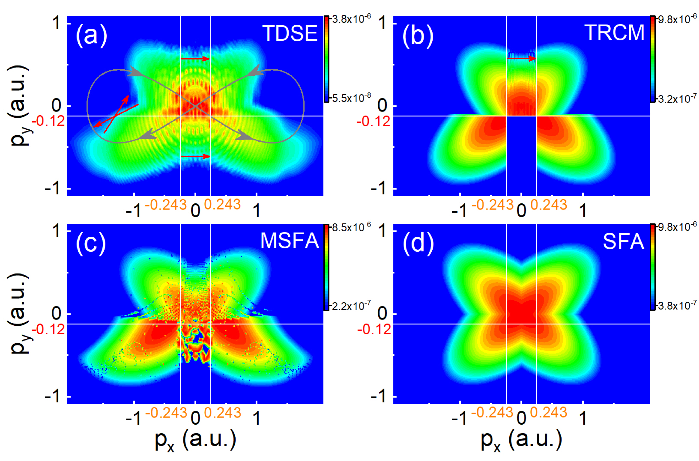
Figure 1: Comparisons of PMD obtained with TDSE (a), TRCM (b), MSFA (c), and SFA (d) in OTC. The prediction of SM (gray line) is also plotted in (a). Laser parameters used are $I_{x}=5\times 10^{14}$ W/cm², $\lambda_{x}=800$ nm and $\varepsilon=0.5$. The $\log_{10}$ scale is used here. In each panel, the vertical lines indicate the axes of $p^{\prime}_{x}=\pm E_{0}\tau$ and the horizontal one indicates the axis of $p^{\prime}_{y}=-E_{1}\tau$ of Eq. (5). Relevant values of $p^{\prime}_{x}$ and $p^{\prime}_{y}$ are denoted with the color numbers. The intersection of the oblique arrows in (a) indicates the position of the shoulder structure and the horizontal arrows indicate the width of the rectangular structure.

Results and discussions.-In Fig. 1, we show the PMDs of He in OTC calculated with different methods. The TDSE results in Fig. 1(a) show a butterfly shape with two smaller upper wings and two larger lower wings. In particular, the PMD of TDSE presents two typical structures. The first one is a rectangular-like structure and is located in the middle part of the whole PMD. It is like the body of the butterfly and the width of this structure can be identified through the relatively flat part between the two upper or lower wings as indicated by the horizontal arrows. The left and the right boundaries of this structure approximately agree with the relation of $p^{\prime}_{x}=\pm E_{0}\tau$ of Eq. (5), as indicated by these two vertical lines.

The second one is a shoulder-like structure and is located at the top of the lower half plane of the PMD. It has a small slope as indicated by the downward oblique arrow. Below the shoulder structure, the fringe of the distribution shows the large gradient, as indicated by the upward oblique arrow. The intersection of these two arrows indicates the shoulder position which agrees with the relation of $p^{\prime}_{y}=-E_{1}\tau$ of Eq. (5), as indicated by the horizontal line. The main features of PMD of TDSE are well reproduced by the TRCM, as shown in Fig. 1(b). Particularly, the positions of these two typical structures predicted by TRCM are in quantitative agreement with the TDSE ones. For clarity, we also indicate these positions with the vertical and horizontal lines in Fig. 1(b).

By comparison, the PMD obtained with the Coulomb-modified SFA (MSFA) model Xie , is similar to the TRCM one, but the positions of these two typical structures differ remarkably from the TRCM predictions of $p^{\prime}_{x}=\pm E_{0}\tau$ and $p^{\prime}_{y}=-E_{1}\tau$, as indicated by the lines. The rectangular structure predicted by the MSFA is narrower than the TRCM one and the position of the shoulder structure is near to the axis of $p_{y}=0$. Different from the TRCM which mainly considers the Coulomb effect near the nucleus with the virial theorem, the MSFA considers the Coulomb effect through numerical solution of the Newton equation including both the electric-field force and the Coulomb force for each SFA electron trajectories after the tunneling electron exits the barrier.

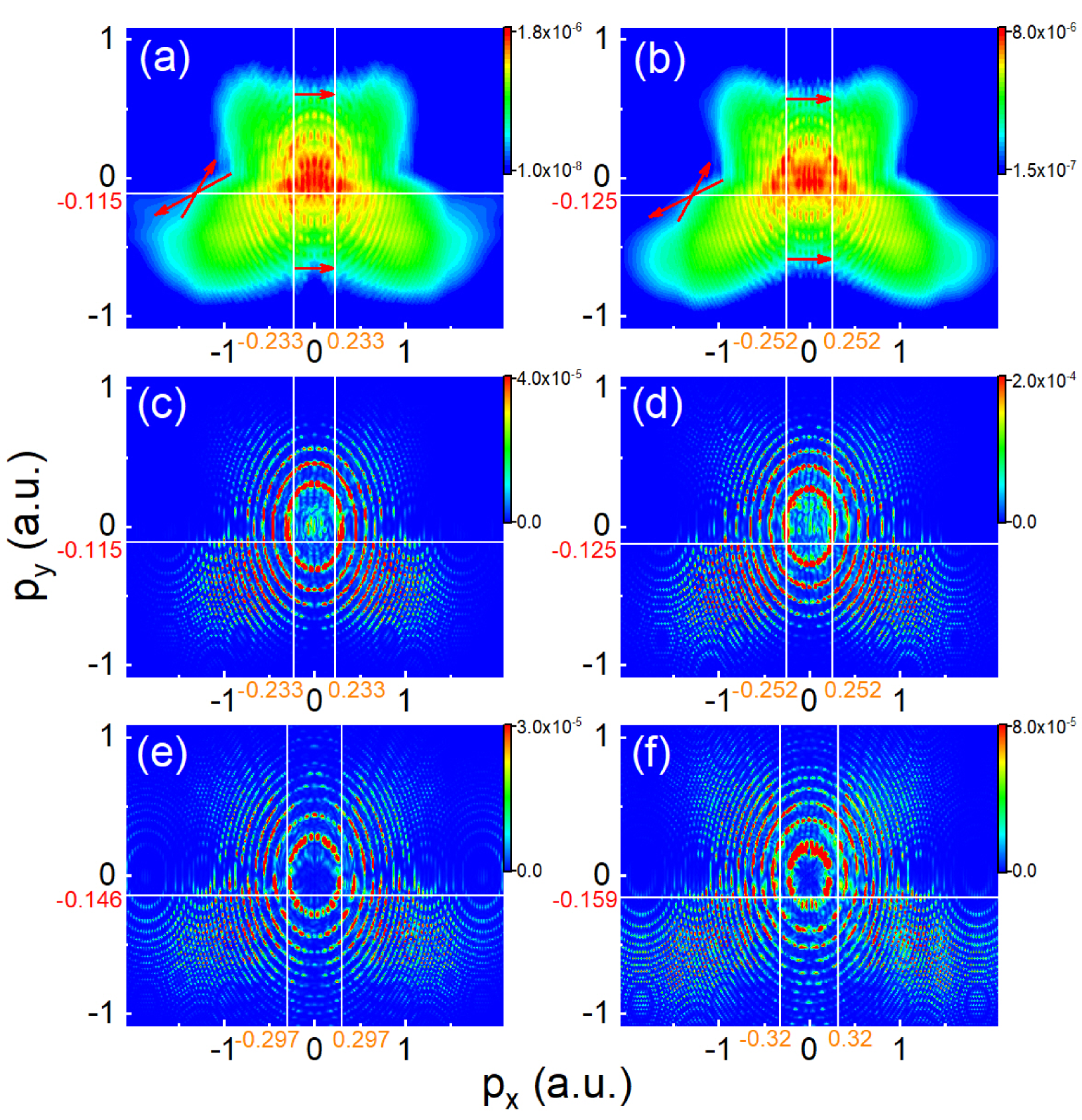
Figure 2: PMDs of He in OTC obtained with TDSE for $I_{x}=4\times 10^{14}$W/cm² (first column) and $I_{x}=6\times 10^{14}$W/cm² (second) in 3D noncoherent (first row) and coherent cases (second) and 2D coherent cases (third). Other laser parameters used are $\lambda_{x}=800$ nm and $\varepsilon=0.5$. The $\log_{10}$ scale is used in the first row. The lines and arrows are as in Fig. 1.

Let us further understand the origin of the butterfly structure of PMD in OTC with the TRCM. The PMD obtained with SFA where the Coulomb effect is not considered is presented in Fig. 1(d). The PMD of SFA shows a high symmetry with respect to both the axes of $p_{x}=0$ and $p_{y}=0$. In addition, the distributions of SFA along these two axes both have large amplitudes. When the Coulomb effect is considered with TRCM, the mapping of Eq. (3) begins to work. In comparison with Eq. (2) of SFA predictions, Eq. (3) shows that the Coulomb effect induces a time lag $\tau$ of the ionization time $t_{i}$ relative to the tunneling-out time $t_{0}$. For $p_{y}\geq 0$, this lag results in the shift of the whole right (left) part of SFA distribution with $p_{x}\geq 0$ ($p_{x}\leq 0$) towards the left (right), and the situation reverses for $p_{y}<0$. In addition, this lag also induces the shift of the entire upper part of SFA distribution towards the lower region. More specifically, this shift follows the direction of the gray arrow for the SM predictions of $\textbf{p}=-\textbf{A}(t)$ plotted in Fig. 1(a). The left and right offsets of the axis $p_{x}=0$ forms the boundaries of the rectangular structure around $p^{\prime}_{x}\approx\pm E_{0}\tau$ and the downward offset of the axis $p_{y}=0$ forms the shoulder structure. Our analyses show that the TRCM predictions of momenta $\textbf{p}^{\prime}$ are similar for SFA momenta p along the axis of $p_{x}=0$ or $p_{y}=0$. Therefore, if the structures can be quantitatively identified in PMD, one may obtain the lag $\tau$ from the positions of the structures with Eq. (5). Then the ionization time (the birth time) $t_{i}=t_{0}+\tau$ of the tunneling electron can be determined. However, the boundary of the rectangular structure is not regular enough due to the interference between the shifted distributions from different parts. By comparison, the shoulder structure is more regular and the position of this structure is easier to determine. To the best of our knowledge, this is the first quantitative explanation on the origin of the butterfly structure of PMD in OTC.

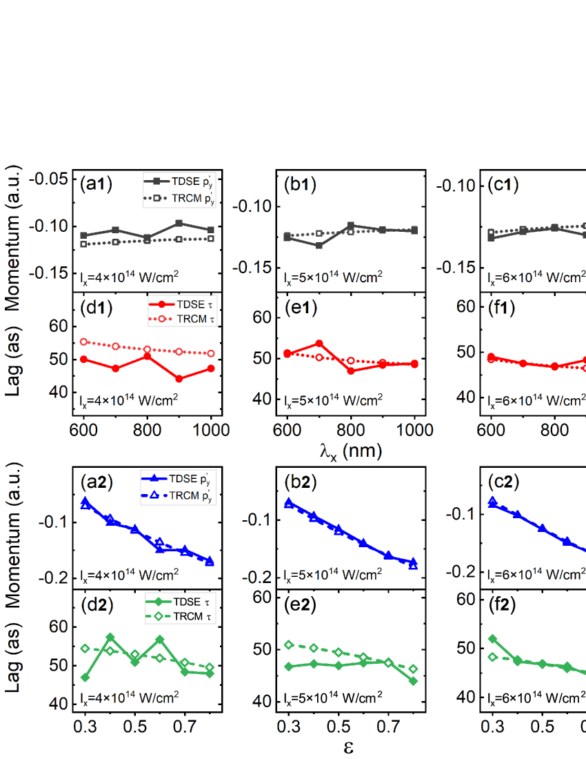
Figure 3: Comparisons of the shoulder position $p^{\prime}_{y}$ in PMD (first and third rows) and the corresponding time lag $\tau$ (second and fourth rows) predicted by TDSE and TRCM for different $\lambda_{x}$ at $\varepsilon=0.5$ (a1-f1) and different $\varepsilon$ at $\lambda_{x}=800$ nm (a2-f2). The laser intensities $I_{x}$ used are as shown. The TDSE shoulder position is obtained as in Fig. 1 and the TRCM one is obtained with $p^{\prime}_{y}=-E_{1}\tau$ of Eq. (5). The corresponding lags are obtained through $\tau\approx\sqrt{|V({\textbf{r}}(t_{0}))|/n_{f}}/\sqrt{E_{0}^{2}+E_{1}^{2}}$ of TRCM predictions and through $\tau=|p^{\prime}_{y}|/E_{1}$ with $|p^{\prime}_{y}|$ being TDSE predictions of the shoulder position.

In Fig. 2, we show PMDs of He in OTC calculated by TDSE with both noncoherent and coherent treatments at different laser intensities. For comparison, coherent results with two-dimensional (2D) simulations are also shown. One can observe that for all of the noncoherent and coherent results in 3D and 2D cases, these two typical structures can be well resolved. The positions of these structure are also in agreement with the TRCM predictions as indicated by the solid lines of $p^{\prime}_{x}=\pm E_{0}\tau$ and $p^{\prime}_{y}=-E_{1}\tau$ of Eq. (5). It is worth noting that although the coherent results show some complex interference structures, the shoulder positions can also be clearly identified from the flat contour of this structure around $p_{x}=\pm 1$ a.u.. Here, no trajectories contributes to the distribution higher than the contour in TRCM (also see Fig. 1(b)). In addition, the position in 2D cases associated with $n_{f}=2$ in Eq. (4) is larger than in 3D cases with $n_{f}=3$. Thirdly, for the present cases, the shoulder position is not very sensitive to the laser intensity.

As the shoulder position can be more easily determined (as shown in Fig. 1 and Fig. 2), in Fig. 3, we compare the TDSE predictions of this position to the theoretical ones at various laser parameters.

In the first row of Fig. 3, we show relevant comparisons at different laser intensities and wavelengths. Firstly, the TDSE and theoretical results agree well with each other for different cases, with an average error smaller than $10\%$. Secondly, for a fixed intensity, the position changes slowly with increasing the wavelength. Thirdly, for a fixed wavelength, the position also shows a slow increase when the laser intensity increases. In the second row of Fig. 3, we show the corresponding time lag $\tau$ obtained with TRCM and TDSE. One can observe that for the present cases, the theoretical prediction of $\tau$ is located at a range of about $45$ to $55$ attoseconds and decreases slowly both for increasing the laser wavelength and intensity. The TDSE results agree well with the theoretical ones with an average difference smaller than $5$ attoseconds. This agreement is more remarkable for higher laser intensities and longer wavelengths $\lambda_{x}$ on the whole.

In the third and the fourth rows of Fig. 3, we show further comparisons for different ratios $\varepsilon$. It can be observed from the third row, the TDSE and TRCM predictions of the shoulder position are in good agreement with each other. In addition, for a fixed laser intensity, the position increases remarkably when increasing the ratio $\varepsilon$, with the position $p^{\prime}_{y}$ changing from $p^{\prime}_{y}\approx-0.07$ a.u. at $\varepsilon=0.3$ to $p^{\prime}_{y}\approx-0.18$ a.u. at $\varepsilon=0.8$. By comparison, the corresponding time lag $\tau$ in the fourth row of Fig. 3 is located at a smaller range as increasing $\varepsilon$. This range is about $50$ to $55$ attoseconds in Fig. 3(d2), $46$ to $51$ attoseconds in Fig. 3(e2) and $43$ to $48$ attoseconds in Fig. 3(f2). The TDSE and theoretical predictions of $\tau$ are still well consistent with each other here, with a difference smaller than $5$ attoseconds. This difference is smaller for cases of higher laser intensities and larger $\varepsilon$, suggesting the preferred laser parameters in experiments.

Conclusion.-In summary, we have studied ionization of He in strong OTC laser fields. The PMDs of He in OTC show two typical structures, i.e., the rectangular one and the shoulder one related to the most probable route. The locations of these two structures encode the response time of electron inside an atom to light in laser induced tunneling ionization. This time can be easily extracted from the position of the shoulder structure that can be well identified in PMD. The OTC laser field has wide applications in manipulating the electron motion in both ATI and HHG. The two-color attosecond chronoscope proposed here provides a simple tool for timing the birth of electron in relevant OTC-based manipulations.

This work was supported by the National Natural Science Foundation of China (Grant Nos. 12174239, 11904072).

Appendix A Numerical Methods

In the length gauge and single-active electron approximation, the Hamiltonian of the He atom interacting with a strong laser field can be written as (in atomic units of $\hbar=e=m_{e}=1$)

$${H}(t)=H_{0}+\mathbf{E}(t)\cdot\mathbf{r}$$ (6)

Here, $H_{0}={\mathbf{{p}}^{2}}/{2}+V(\mathbf{r})$ is the field-free Hamiltonian and $V(\textbf{r})=-Z/\sqrt{r^{2}+\xi}$ is the Coulomb potential with the effective charge $Z$ and the soft-core parameter $\xi$. In three-dimensional (3D) cases, we have used the parameters of $Z=1.34$ and $\xi=0.071$. With these parameters, the ionization potential of He reproduced is $I_{p}=0.9$ a.u.. The term $\mathbf{E}(t)$ denotes the electric field of the OTC laser field as introduced in the main text.

We use trapezoidally shaped laser pulses with a total duration of fifteen cycles, which are linearly turned on and off for three optical cycles, and then kept at a constant intensity for nine additional cycles. The TDSE of $i\dot{\Psi}(\textbf{r},t)=$H$(t)\Psi(\textbf{r},t)$ is solved numerically using the spectral method Feit with a time step of $\triangle t=0.05$ a.u.. We have used a grid size of $L_{x}\times L_{y}\times L_{z}=358.4\times 358.4\times 51.2$ a.u. with $\triangle x=\triangle y=0.7$ a.u. and $\triangle z=0.8$ a.u.. The numerical convergence is checked by using a finer grid.

In order to avoid the reflection of the electron wave packet from the boundary and obtain the momentum space wavefunction, the coordinate space is split into the inner and the outer regions with ${\Psi}(\textbf{r},t)={\Psi}_{in}(\textbf{r},t)+{\Psi}_{out}(\textbf{r},t)$, by multiplying a mask function of $F(\mathbf{r})$. The mask function has the form of $F(\mathbf{r})=F_{1}(x)F_{2}(y)F_{3}(z)$. Here, $F_{1}(x)=\cos^{1/8}[\pi(|{x}|-r_{x})/(L_{x}-2r_{x})]$ for $|{x}|\geq r_{x}$ and $F_{1}(x)=1$ for $|{x}|<r_{x}$. $r_{x}=134$ a.u. is the absorbing boundary. The form of $F_{2}(y)$ is similar to $F_{1}(x)$. The expression of $F_{3}(z)$ is also similar to $F_{1}(x)$ but the absorbing boundary along the $z$ direction is $r_{z}=19.2$ a.u.. In the inner region, the wave function ${\Psi}_{in}(\textbf{r},t)$ is propagated with the complete Hamiltonian $H(t)$. In the outer region, the time evolution of the wave function ${\Psi}_{out}(\textbf{r},t)$ is carried out in momentum space with the Hamiltonian of the free electron in the laser field. The mask function is applied at each time interval of 0.5 a.u. and the obtained new fractions of the outer wave function are noncoherently (coherently) added to the momentum-space wave function $\tilde{{\Psi}}_{out}(\textbf{r},t)$ from which we obtain the noncoherent (coherent) PMD.

For comparison with 3D results, we have also performed two-dimensional (2D) simulations. In 2D cases, we have used the parameters of $Z=1.45$ and $\xi=0.5$ for the potential $V(\textbf{r})=-Z/\sqrt{r^{2}+\xi}$. The grid size used in 2D cases is $L_{x}\times L_{y}=409.6\times 409.6$ a.u. with space steps of $\triangle x=\triangle y=0.4$ a.u.. The mask function used is $F(\mathbf{r})=F_{1}(x)F_{2}(y)$. The forms of $F_{1}(x)$ and $F_{2}(y)$ are similar to 3D cases with the absorbing boundary of $r_{x}=r_{y}=150$ a.u..

References

- (1) P. B. Corkum and F. Krausz, Attosecond science, Nature Phys. 3, 381 (2007).
- (2) F. Krausz and M. Ivanov, Attosecond physics, Rev. Mod. Phys. 81, 163 (2009).
- (3) J. M. Dahlström, A. L’Huillier, and A. Maquet, Introduction to attosecond delays in photoionization, J. Phys. B 45, 183001 (2012).
- (4) F. Lépine, M. Y. Ivanov, and M. J. J. Vrakking, Attosecond molecular dynamics: fact or fiction? Nature Photon. 8, 195 (2014).
- (5) R. Pazourek, S. Nagele, J. Burgdörfer, Attosecond chronoscopy of photoemission, Rev. Mod. Phys. 87, 765 (2015).
- (6) J. Vos, L. Cattaneo, S. Patchkovskii, T. Zimmermann, C. Cirelli, M. Lucchini, A. Kheifets, A. S. Landsman, U. Keller, Orientation-dependent stereo Wigner time delay and electron localization in a small molecule, Science 360, 1326 (2018).
- (7) P. B. Corkum, Plasma perspective on strong field multiphoton ionization, Phys. Rev. Lett. 71, 1994 (1993).
- (8) L. V. Keldysh, Ionization in the field of a strong electromagnetic wave, Sov. Phys. JETP 20, 1307 (1965).
- (9) P. Agostini, F. Fabre, G. Mainfray, G. Petite, and N. K. Rahman, Free-Free Transitions Following Six-Photon Ionization of Xenon Atoms, Phys. Rev. Lett. 42, 1127 (1979).
- (10) B. Yang, K. J. Schafer, B. Walker, K. C. Kulander, P. Agostini, and L. F. DiMauro, Intensity-dependent scattering rings in high order above-threshold ionization, Phys. Rev. Lett. 71, 3770 (1993).
- (11) G. G. Paulus, W. Becker, W. Nicklich, and H. Walther, Rescattering effects in above-threshold ionization: a classical model, J. Phys. B 27, L703 (1994).
- (12) M. Lewenstein, K. C. Kulander, K. J. Schafer, and P. H. Bucksbaum, Rings in above-threshold ionization: A quasiclassical analysis, Phys. Rev. A 51, 1495 (1995).
- (13) W. Becker, F. Grasbon, R. Kopold, D. B. Milos̆ević, G. G. Paulus, and H. Walther, Above-threshold ionization: from classical features to quantum effects, Adv. At. Mol. Opt. Phys. 48, 35 (2002).
- (14) A. McPherson, G. Gibson, H. Jara, U. Johann, T. S. Luk, I. A. McIntyre, K. Boyer, and C. K. Rhodes, Studies of multiphoton production of vacuum-ultraviolet radiation in the rare gases, J. Opt. Soc. Am. B 4, 595(1987).
- (15) A. L’Huillier, K. J. Schafer, and K. C. Kulander, Theoretical aspects of intense field harmonic generation, J. Phys. B 24, 3315 (1991).
- (16) M. Lewenstein, Ph. Balcou, M. Yu. Ivanov, A. L’Huillier, and P. B. Corkum, Theory of high-harmonic generation by low-frequency laser fields, Phys. Rev. A 49, 2117 (1994).
- (17) N. Dudovich, O. Smirnova, J. Levesque, Y. Mairesse, M. Y. Ivanov, D. M. Villeneuve, and P. B. Corkum, Measuring and controlling the birth of attosecond XUV pulses, Nat. Phys. 2, 781 (2006).
- (18) Z. Zeng, Y. Cheng, X. Song, R. Li, and Z. Xu, Generation of an Extreme Ultraviolet Supercontinuum in a Two-Color Laser Field, Phys. Rev. Lett. 98, 203901 (2007).
- (19) H. Mashiko, S. Gilbertson, C. Li, S. D. Khan, M. M. Shakya, E. Moon, and Z. Chang, Double Optical Gating of High-Order Harmonic Generation with Carrier-Envelope Phase Stabilized Lasers, Phys. Rev. Lett. 100, 103906 (2008).
- (20) Y. Z. Shi, S. Wang, F. L. Dong, Y. P. Li, and Y. J. Chen, Classical effect for enhanced high harmonic yield in ultrashort laser pulses with a moderate laser intensity, J. Phys. B 50, 065004 (2017).
- (21) P. Eckle, M. Smolarski, P. Schlup, J. Biegert, A. Staudte, M. Schöffler, H. G. Muller, R. Dörner, and U. Keller, Attosecond angular streaking, Nat. Phys. 4, 565-570 (2008).
- (22) P. Eckle, A. N. Pfeiffer, C. Cirelli, A. Staudte, R. Dörner, H. G. Muller, M. Büttiker, and U. Keller, Attosecond ionization and tunneling delay time measurements in helium, Science 322, 1525-1529 (2008).
- (23) A. N. Pfeiffer, C. Cirelli, M. Smolarski, D. Dimitrovski, M. Abu-samha, L. B. Madsen, and U. Keller, Attoclock reveals natural coordinates of the laser-induced tunnelling current flow in atoms, Nat. Phys. 8, 76-80 (2012).
- (24) R. Boge, C. Cirelli, A. S. Landsman, S. Heuser, A. Ludwig, J. Maurer, M. Weger, L. Gallmann, and U. Keller, Probing Nonadiabatic Effects in Strong-Field Tunnel Ionization, Phys. Rev. Lett. 111, 103003 (2013).
- (25) L. Torlina, F. Morales, J. Kaushal, I. Ivanov, A. Kheifets, A. Zielinski, A. Scrinzi, H. G. Muller, S. Sukiasyan, M. Ivanov, and O. Smirnova, Interpreting attoclock measurements of tunnelling times, Nat. Phys. 11, 503-508 (2015).
- (26) W. Quan, V. V. Serov, M. Z. Wei, M. Zhao, Y. Zhou, Y. L. Wang, X. Y. Lai, A. S. Kheifets, and X. J. Liu, Attosecond Molecular Angular Streaking with All-Ionic Fragments Detection, Phys. Rev. Lett. 123, 223204 (2019).
- (27) U. S. Sainadh, H. Xu, X. Wang, A. Atia-Tul-Noor, W. C. Wallace, N. Douguet, A. Bray, I. Ivanov, K. Bartschat, A. Kheifets, R. T. Sang, and I. V. Litvinyuk, Attosecond angular streaking and tunnelling time in atomic hydrogen, Nature (London) 568, 75-77 (2019).
- (28) M. Kitzler and M. Lezius, Spatial Control of Recollision Wave Packets with Attosecond Precision, Phys. Rev. Lett. 95, 253001 (2005).
- (29) L. Brugnera, D. J. Hoffmann, T. Siegel, F. Frank, A. Zaïr, J. W. G. Tisch, and J. P. Marangos, Trajectory Selection in High Harmonic Generation by Controlling the Phase between Orthogonal Two-Color Fields, Phys. Rev. Lett. 107, 153902 (2011).
- (30) M. Kitzler, X. Xie, A. Scrinzi, and A. Baltuska, Optical attosecond mapping by polarization selective detection, Phys. Rev. A 76, 011801 (2007).
- (31) D. Shafir, Y. Mairesse, D. M. Villeneuve, P. B. Corkum, and N. Dudovich, Atomic wavefunctions probed through strong-field light-matter interaction, Nat. Phys. 5, 412 (2009).
- (32) D. Shafir, H. Soifer, B. D. Bruner, M. Dagan, Y. Mairesse, S. Patchkovskii, M. Yu. Ivanov, O. Smirnova, and N, Dudovich, Resolving the time when an electron exits a tunnelling barrier, Nature 485, 343 (2012).
- (33) J. Zhao and M. Lein, Determination of Ionization and Tunneling Times in High-Order Harmonic Generation, Phys. Rev. Lett. 111, 043901 (2013).
- (34) C. Chen, D. X. Ren, X. Han, S. P. Yang, and Y. J. Chen, Time-resolved harmonic emission from aligned molecules in orthogonal two-color fields, Phys. Rev. A 98, 063425 (2018).
- (35) X. J. Xie, C. Chen, G. G. Xin, J. Liu, and Y. J. Chen, Coulomb-induced ionization time lag after electrons tunnel out of a barrier, Opt. Express 28, 33228 (2020).
- (36) M. D. Feit, J. A. Fleck, Jr., and A. Steiger, Solution of the Schrdinger Equation by a Spectral Method, J. Comput. Phys. 47, 412 (1982).
- (37) See numerical methods in the appendix.
- (38) J. Y. Che, C. Chen, W. Y. Li, S. Wang, X. J. Xie, J. Y. Huang, Y. G. Peng, G. G. Xin, and Y. J. Chen, Response time of photoemission at quantum-classic boundary, arXiv:2111.08491 (2021).
- (39) T. Brabec, M. Yu. Ivanov, and P. B. Corkum, Coulomb focusing in intense field atomic processes, Phys. Rev. A 54, R2551 (1996).
- (40) S. P. Goreslavski, G. G. Paulus, S. V. Popruzhenko, and N. I. Shvetsov-Shilovski, Coulomb Asymmetry in Above-Threshold Ionization, Phys. Rev. Lett. 93, 233002 (2004).
- (41) T. M. Yan, S. V. Popruzhenko, M. J. J. Vrakking, and D. Bauer, Low-energy structures in strong field ionization revealed by quantum orbits, Phys. Rev. Lett. 105, 253002 (2010).
- (42) S. Wang, J. Y. Che, C. Chen, G. G. Xin, and Y. J. Chen, Tracing the origins of an asymmetric momentum distribution for polar molecules in strong linearly polarized laser fields, Phys. Rev. A 102, 053103 (2020).
- (43) C. Chen, X. X. Ji, W. Y. Li, X. Han, and Y. J. Chen, Local most-probable routes and classic-quantum correspondence in strong-field two-dimensional tunneling ionization, Phys. Rev. A 104, 013106 (2021).
- (44) These authors contribute equally to this paper.
- (45) liweiyanhb@126.com
- (46) chenyjhb@gmail.com