Don’t Play Favorites: Minority Guidance for Diffusion Models

Abstract

We explore the problem of generating minority samples using diffusion models. The minority samples are instances that lie on low-density regions of a data manifold. Generating sufficient numbers of such minority instances is important, since they often contain some unique attributes of the data. However, the conventional generation process of the diffusion models mostly yields majority samples (that lie on high-density regions of the manifold) due to their high likelihoods, making themselves highly ineffective and time-consuming for the task. In this work, we present a novel framework that can make the generation process of the diffusion models focus on the minority samples. We first provide a new insight on the majority-focused nature of the diffusion models: they denoise in favor of the majority samples. The observation motivates us to introduce a metric that describes the uniqueness of a given sample. To address the inherent preference of the diffusion models w.r.t. the majority samples, we further develop minority guidance, a sampling technique that can guide the generation process toward regions with desired likelihood levels. Experiments on benchmark real datasets demonstrate that our minority guidance can greatly improve the capability of generating the low-likelihood minority samples over existing generative frameworks including the standard diffusion sampler.

1 Introduction

Conventional large-scale datasets are mostly long-tailed in their distributions, containing the minority of samples in low-probability regions of a data manifold (Ryu et al., 2017; Liu et al., 2019). The minority samples often comprise novel attributes rarely observed in majority samples lying in high-density regions which usually consist of common features of the data (Agarwal et al., 2022). Generating enough numbers of the minorities is important in well representing a given dataset, and more crucially, in reducing the negative societal impacts of generative models in terms of fairness (Choi et al., 2020; Xiao et al., 2021).

One challenge is that generation focused on such minority samples is actually difficult to perform (Hendrycks et al., 2021). This holds even for diffusion-based generative models (Sohl-Dickstein et al., 2015; Ho et al., 2020) that provide strong coverage for a given data distribution (Sehwag et al., 2022). The generation process of the diffusion models can be understood as simulating the reverse of a diffusion process that defines a set of noise-perturbed data distributions (Song & Ermon, 2019), which guarantees their samples to respect the (clean) data distribution when a properly-learned score function is available (e.g., via denoising score-matching (DSM) (Vincent, 2011)). Given the long-tail-distributed data, such probabilistic faithfulness of the diffusion models makes their sampler become majority-oriented, i.e., producing higher likelihood samples more frequently than lower likelihood ones (Sehwag et al., 2022).

Contribution. In this work, we provide a new perspective on the majority-focused aspect of diffusion models. Specifically, we investigate the denoising behavior of diffusion models over samples with various features and show that diffusion models, when obtained via DSM, play favorites with majorities: their reconstruction (w.r.t. given noised input) favors to produce common-featured samples over ones containing unique features. Surprisingly, we find that even when perturbations are made upon the unique-featured samples (so we naturally expect denoising back to the ones having the same novel features), the diffusion models often produce reconstruction to the common-featured majority samples, thereby yielding significant semantic changes in the reconstructed versions of the minority samples (see Figure 1 for instance). This motivates us to come up with a new metric for describing the uniqueness of features contained in a given sample, which we call minority score, defined as a perceptual distance (e.g., LPIPS (Zhang et al., 2018)) between the original and restored instances. We highlight that our metric is efficient to compute, being sufficient with one-shot reconstruction given by Tweedie’s formula (Stein, 1981; Robbins, 1992; Efron, 2011).

Given the proposed metric at hand, we further develop a sampling technique for addressing the inherent preference of the diffusion models toward the majority features. Our sampler, which we call minority guidance, makes the sampling process condition on a desired level of minority score. More precisely, we construct a classifier that predicts (discretized) minority scores for given perturbed input and incorporate it into a conventional sampler (e.g., ancestral sampling (Sohl-Dickstein et al., 2015; Ho et al., 2020)) using the classifier guidance (Dhariwal & Nichol, 2021). We find that our minority guidance enables a controllable generation of the minority-featured samples, e.g., by conditioning on high minority score in our sampler.

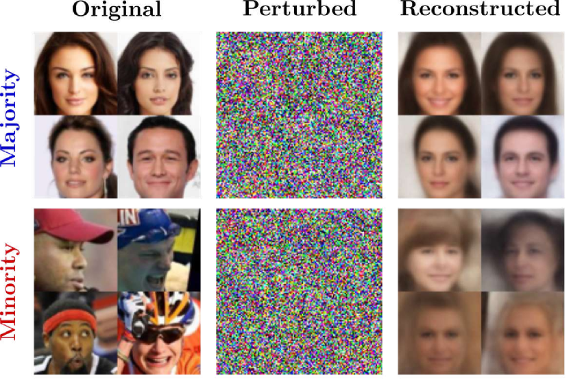
Figure 1: Diffusion models play favorites with majority features. (Left column) Clean images from CelebA (Liu et al., 2015); (Middle column) Noise-corrupted samples made by the DDPM perturbation (1) on the clean samples in the left column; (Right column) Denoised samples using Tweedie’s formula (5) on the perturbed ones. The top (bottom) row represents the perturbation-reconstruction process for majority (minority) featured samples.

We conduct extensive experiments on various benchmark real datasets. We demonstrate that minority score can serve to identify samples with novel features in a given dataset. We also exhibit that our minority guidance can serve as an effective knob for controlling the uniqueness of features for generated samples. We observe that our sampler can greatly improve the capability of generating the minority samples over existing generative samplers including ancestral sampling, reflected in high values of outlier measures like Average k-Nearest Neighbor and Local Outlier Factor (Breunig et al., 2000).

Related work. Generating minority samples that contain novel features has been explored under a number of different scenarios (Sehwag et al., 2022; Lin et al., 2022; Yu et al., 2020; Lee et al., 2022). The closest instance to our work is Sehwag et al. (2022) wherein the authors propose a sampling technique for diffusion models, which can encourage the generation process to move toward low-density regions (for a specific class) using a class-predictor and a conditional model. The key distinction w.r.t. ours is that their method is limited to class-conditional settings and requires access to class labels. Another notable work that bears an intimate connection to ours is Lee et al. (2022). As in Sehwag et al. (2022), they also leverage diffusion models yet for a different modality, graph data (e.g., lying in chemical space). The key idea therein is to produce out-of-distribution (OOD) samples via a customized generation process designed for maintaining some desirable properties w.r.t. the focused data space (e.g., plausible chemical structures). Since it is tailored for a particular modality which is inherently distinct from our focus (e.g., image data), hence not directly comparable to our approach.

Leveraging diffusion models for detecting uncommon instances (e.g., OOD samples) has recently been proposed, especially for medical imaging (Wolleb et al., 2022; Wyatt et al., 2022; Teng et al., 2022). Their methods share a similar spirit as ours: measuring discrepancies between the original and reconstructed images. However, they rely upon heuristic intuitions in designing their proposals and does not provide any theoretical supports for them. Also, their methods require a number of function evaluations (of diffusion models), thus computationally more expensive than ours.

After firstly introduced in Sohl-Dickstein et al. (2015), the classifier guidance has been a gold standard for imposing class-conditions into the generation process of diffusion models. Its use cases range far and wide, from high-quality sample generation (Dhariwal & Nichol, 2021) to text-to-speech synthesis (Kim et al., 2022), anomaly detection for medical images (Wolleb et al., 2022), and so on. To our best knowledge, the proposed approach is the first attempt that leverages the classifier guidance for incorporating conditions w.r.t. the novelty of features in the generation process.

2 Background

Before going into details of our work, we briefly review several key elements of diffusion-based generative models. We provide an overview of diffusion models with a particular focus on Denoising Diffusion Probabilistic Models (DDPM) (Ho et al., 2020) that our framework is based upon. Also, we review the classifier guidance (Dhariwal & Nichol, 2021) which provides a basic principle for our sampling technique.

2.1 Diffusion-based generative models

Diffusion-based generative models (Sohl-Dickstein et al., 2015; Song & Ermon, 2019) are latent variable models defined by a forward diffusion process and the associated reverse process. The forward process is a Markov chain with a Gaussian transition where data is gradually corrupted by Gaussian noise in accordance with a (positive) variance schedule $\{{\beta_{t}}\}_{t=1}^{T}$:

$$q({\boldsymbol{x}}_{t}\mid{\boldsymbol{x}}_{t-1})\coloneqq{\cal N}({\boldsymbol{x}}_{t};\sqrt{1-\beta_{t}}{\boldsymbol{x}}_{t-1},\beta_{t}{\boldsymbol{I}}),$$

where $\{{\boldsymbol{x}}_{t}\}_{t=1}^{T}$ are latent variables having the same dimensionality as the data ${\boldsymbol{x}}_{0}\sim q({\boldsymbol{x}}_{0})$. One notable property is that the forward process enables one-shot sampling of ${\boldsymbol{x}}_{t}$ at any desired timestep $t$:

$$q_{\alpha_{t}}({\boldsymbol{x}}_{t}\mid{\boldsymbol{x}}_{0})={\cal N}({\boldsymbol{x}}_{t};\sqrt{\alpha_{t}}{\boldsymbol{x}}_{0},(1-\alpha_{t}){\boldsymbol{I}}),$$ (1)

where $\alpha_{t}\coloneqq\prod_{s=1}^{t}(1-\beta_{s})$. The variance schedule is designed to respect $\alpha_{T}\approx 0$ so that ${\boldsymbol{x}}_{T}$ becomes approximately distributed as ${\cal N}(\boldsymbol{0},\boldsymbol{I})$. The reverse process is another Markov Chain that is parameterized by a learnable Gaussian transition:

$$p_{\boldsymbol{\theta}}({\boldsymbol{x}}_{t-1}\mid{\boldsymbol{x}}_{t})\coloneqq{\cal N}({\boldsymbol{x}}_{t-1};\boldsymbol{\mu}_{\boldsymbol{\theta}}({\boldsymbol{x}}_{t},t),\beta_{t}{\boldsymbol{I}}).$$

One way to express $\boldsymbol{\mu}_{\boldsymbol{\theta}}({\boldsymbol{x}}_{t},t)$ is to employ a noise-conditioned score network ${\boldsymbol{s}}_{\boldsymbol{\theta}}({\boldsymbol{x}}_{t},t)\coloneqq\nabla_{{\boldsymbol{x}}_{t}}\log p_{\boldsymbol{\theta}}({\boldsymbol{x}}_{t})$ that approximates the score function $\nabla_{{\boldsymbol{x}}_{t}}\log q_{\alpha_{t}}({\boldsymbol{x}}_{t})$: $\boldsymbol{\mu}_{\boldsymbol{\theta}}({\boldsymbol{x}}_{t},t)=\frac{1}{\sqrt{1-\beta_{t}}}({\boldsymbol{x}}_{t}+\beta_{t}{\boldsymbol{s}}_{\boldsymbol{\theta}}({\boldsymbol{x}}_{t},t))$ (Song & Ermon, 2019; Song et al., 2020b). The score network is trained with a weighted sum of denoising score matching (DSM) (Vincent, 2011) objectives:

$$\min_{{\boldsymbol{\theta}}}\sum_{t=1}^{T}w_{t}\mathbb{E}_{q({\boldsymbol{x}})q_{\alpha_{t}}(\tilde{{\boldsymbol{x}}}\mid{\boldsymbol{x}})}[\|{\boldsymbol{s}}_{\boldsymbol{\theta}}(\tilde{{\boldsymbol{x}}},t)-\nabla_{\tilde{\boldsymbol{x}}}\log q_{\alpha_{t}}(\tilde{\boldsymbol{x}}\mid{\boldsymbol{x}})\|_{2}^{2}],$$ (2)

where $w_{t}\coloneqq 1-\alpha_{t}$. Notably, this procedure is equivalent to building a noise-prediction network ${\boldsymbol{\epsilon}_{\theta}}({\boldsymbol{x}}_{t},t)$ that regresses noise added on clean data ${\boldsymbol{x}}_{0}$ through the forward process (1) (Vincent, 2011; Song et al., 2020b). This establishes an intimate connection between the two networks: ${\boldsymbol{s}}_{\boldsymbol{\theta}}({\boldsymbol{x}}_{t},t)=-{\boldsymbol{\epsilon}_{\theta}}({\boldsymbol{x}}_{t},t)/\sqrt{1-\alpha_{t}}$, implying that the score model is actually a denoiser.

Once obtaining the optimal model via the DSM training, data generation can be done by starting from ${\boldsymbol{x}}_{T}\sim{\cal N}({\boldsymbol{0}},{\boldsymbol{I}})$ and following the reverse Markov Chain down to ${\boldsymbol{x}}_{0}$:

$${\boldsymbol{x}}_{t-1}=\frac{1}{\sqrt{1-\beta_{t}}}({\boldsymbol{x}}_{t}+\beta_{t}{\boldsymbol{s}}_{\boldsymbol{\theta}}({\boldsymbol{x}}_{t},t))+\beta_{t}{\boldsymbol{z}},\;\;\;{\boldsymbol{z}}\sim{\cal N}({\boldsymbol{0}},{\boldsymbol{I}}),$$ (3)

which is often called ancestral sampling (Song et al., 2020b). This process corresponds to a discretized simulation of a stochastic differential equation that defines $\{p_{\boldsymbol{\theta}}({\boldsymbol{x}}_{t})\}_{t=0}^{T}$ (Song et al., 2020b), which guarantees to sample from $p_{\boldsymbol{\theta}}({\boldsymbol{x}}_{0})\approx q({\boldsymbol{x}}_{0})$.

2.2 Classifier guidance for diffusion models

Suppose we have access to auxiliary classifier $p_{\boldsymbol{\phi}}(y|{\boldsymbol{x}}_{t})$ that predicts class $y$ given perturbed input ${\boldsymbol{x}}_{t}$. The main idea of the classifier guidance is to construct the score function of a conditional density w.r.t. $y$ by mixing the score model ${\boldsymbol{s}}_{\boldsymbol{\theta}}({\boldsymbol{x}}_{t},t)$ and the log-gradient of the auxiliary classifier:

$$\begin{split}\nabla_{{\boldsymbol{x}}_{t}}\log\tilde{p}_{\boldsymbol{\theta}}({\boldsymbol{x}}_{t}\mid y)&=\nabla_{{\boldsymbol{x}}_{t}}\{\log p_{\boldsymbol{\theta}}({\boldsymbol{x}}_{t})+\log p_{\boldsymbol{\phi}}(y|{\boldsymbol{x}}_{t})^{w}\}\\ &={\boldsymbol{s}}_{\boldsymbol{\theta}}({\boldsymbol{x}}_{t},t)+w\nabla_{{\boldsymbol{x}}_{t}}\log p_{\boldsymbol{\phi}}(y|{\boldsymbol{x}}_{t})\\ &\eqqcolon\tilde{{\boldsymbol{s}}}_{\boldsymbol{\theta}}({\boldsymbol{x}}_{t},t,y),\end{split}$$ (4)

where $w$ is a hyperparameter that controls the strength of the classifier guidance. Employing the mixed score $\tilde{{\boldsymbol{s}}}_{\boldsymbol{\theta}}({\boldsymbol{x}}_{t},t,y)$ in place of ${\boldsymbol{s}}_{\boldsymbol{\theta}}({\boldsymbol{x}}_{t},t)$ in the generation process (e.g., in (3)) enables the conditional sampling w.r.t. $\tilde{p}_{\boldsymbol{\theta}}({\boldsymbol{x}}_{t}|y)\propto p_{\boldsymbol{\theta}}({\boldsymbol{x}}_{t})p_{\boldsymbol{\phi}}(y|{\boldsymbol{x}}_{t})^{w}$. Increasing the scaling factor $w$ affects the curvature of $p_{\boldsymbol{\phi}}(y|{\boldsymbol{x}}_{t})^{w}$ around given $y$ to be more sharp, i.e., gives more strong focus on some noticeable features w.r.t. $y$, which often yields improvement of fidelity w.r.t. the corresponding class at the expense of diversity (Dhariwal & Nichol, 2021).

3 Method

We present our framework herein that specifically focuses on generating minority samples lying on low-density regions of a data manifold. To this end, we first show that denoising of diffusion models are biased to majority samples having high-likelihoods, which sheds light in a new direction on why diffusion models struggle in the minority-focused generation. In light of this, we come up with a measure for describing the uniqueness of features and then develop a sampler that can guide the generation process of diffusion models toward the minority samples. Throughout the section, we follow the setup and notations presented in Section 2.

3.1 Diffusion models play favorites with majorities

We start by investigating how denoising diffusion models work for samples featured with different levels of uniqueness. Let us consider two distinct samples drawn from the data distribution: ${\boldsymbol{x}}_{0}^{M},{\boldsymbol{x}}_{0}^{m}\sim q({\boldsymbol{x}}_{0})$. Here we assume that ${\boldsymbol{x}}_{0}^{M}$ is a majority sample containing commonly observed attributes, such as frontal-view faces in CelebA (Liu et al., 2015). In addition, ${\boldsymbol{x}}_{0}^{m}$ is assumed as an instance of minorities consisting of novel features, e.g., side-view faces in CelebA. We perturb these points using the DDPM forward process (1) to obtain ${\boldsymbol{x}}_{t}^{M}$ and ${\boldsymbol{x}}_{t}^{m}$ respectively. Then by employing the score model ${\boldsymbol{s}}_{\boldsymbol{\theta}}({\boldsymbol{x}}_{t},t)$ trained on $q({\boldsymbol{x}}_{0})$ with DSM (2), we reconstruct the perturbed samples back to their clean versions in one-shot with Tweedie’s formula (Stein, 1981; Robbins, 1992; Efron, 2011). For instance, ${\boldsymbol{x}}_{t}^{M}$ is denoised as:

$$\hat{{\boldsymbol{x}}}_{0}^{M}\coloneqq\frac{1}{\sqrt{\alpha_{t}}}\left({\boldsymbol{x}}^{M}_{t}+(1-\alpha_{t}){\boldsymbol{s}}_{\boldsymbol{\theta}}({\boldsymbol{x}}^{M}_{t},t)\right).$$ (5)

Similarly, we get $\hat{{\boldsymbol{x}}}_{0}^{m}\coloneqq\frac{1}{\sqrt{\alpha_{t}}}({\boldsymbol{x}}^{m}_{t}+(1-\alpha_{t}){\boldsymbol{s}}_{\boldsymbol{\theta}}({\boldsymbol{x}}^{m}_{t},t))$. Figure 1 illustrates an example of this perturbation-restoration process for groups of majority and minority samples. As we can see, the process yields semantic changes for both groups. However, we observe more significant differences w.r.t. the minority samples where the novel features that are originally contained in their clean versions are replaced with some commonly-observable majority features in the reconstructed samples. This implies that denoising diffusion models actually play favorites with the majority features, i.e., they are biased to produce samples with common attributes from given noisy data instances.

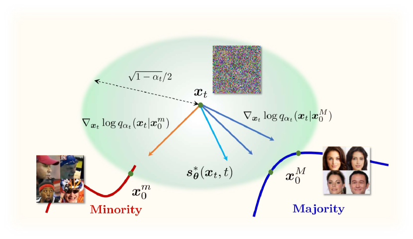
Figure 2: Geometric interpretation of the optimal score model ${\boldsymbol{s}}_{\boldsymbol{\theta}}^{*}({\boldsymbol{x}}_{t},t)=\mathbb{E}_{q({\boldsymbol{x}}_{0}|{\boldsymbol{x}}_{t})}\left[\nabla_{{\boldsymbol{x}}_{t}}\log{q_{\alpha_{t}}({\boldsymbol{x}}_{t}|{\boldsymbol{x}}_{0})}\right]$ derived in Proposition 3.1. The red (blue) curve indicates the data manifold w.r.t. minority (majority) samples. ${\boldsymbol{x}}_{0}^{m}$ and ${\boldsymbol{x}}_{0}^{M}$ denote instances of minority and majority samples, respectively. ${\boldsymbol{x}}_{t}$ is a noised data point (via the DDPM perturbation (1) with timestep $t$) that is possibly corrupted from both ${\boldsymbol{x}}_{0}^{m}$ and ${\boldsymbol{x}}_{0}^{M}$. The orange arrow indicates a conditional score function w.r.t. ${\boldsymbol{x}}_{0}^{m}$, and the dark-blue arrows represent conditional score functions on the (two) majority samples. The light-blue arrow corresponds to the optimal score, i.e., the average of the three conditional score functions.

Now the question is where such preference to the majorities comes from. We found the answer in a routine that we usually adopt for training the diffusion-based models: the DSM optimization. The principle of DSM is approximating the (marginal) score function $\nabla_{{\boldsymbol{x}}_{t}}\log q_{\alpha_{t}}({\boldsymbol{x}}_{t})$ in an average sense by matching a (conditional) score function $\nabla_{{\boldsymbol{x}}_{t}}\log q_{\alpha_{t}}({\boldsymbol{x}}_{t}|{\boldsymbol{x}}_{0})$ over given data ${\boldsymbol{x}}_{0}\sim q({\boldsymbol{x}}_{0})$ (Vincent, 2011). This averaging nature encourages DSM to yield the optimal score model pointing to regions that the majority of samples lies on, rather than to regions w.r.t. the minority samples that rarely contribute to the averaged conditional score due to their small numbers in the given data. To show this idea more clearly, we provide in Proposition 3.1 below a closed-form expression for the optimal score model ${\boldsymbol{s}}^{*}_{\boldsymbol{\theta}}({\boldsymbol{x}}_{t},t)$ yielded by our focused DSM objective (2).

Proposition 3.1.

Consider the DSM optimization in (2). Assume that a given noise-conditioned score network ${\boldsymbol{s}}_{\boldsymbol{\theta}}({\boldsymbol{x}}_{t},t)$ have enough capacity. Then for each timestep $t$, the optimality of the score network is achievable at:

$${\boldsymbol{s}}^{*}_{\boldsymbol{\theta}}({\boldsymbol{x}}_{t},t)=\mathbb{E}_{q({\boldsymbol{x}}_{0}\mid{\boldsymbol{x}}_{t})}\left[\nabla_{{\boldsymbol{x}}_{t}}\log{q_{\alpha_{t}}({\boldsymbol{x}}_{t}\mid{\boldsymbol{x}}_{0})}\right].$$

See Appendix A for the proof. Observe that the optimal model gives the averaged conditional score over the data distribution (conditioned on noised input ${\boldsymbol{x}}_{t}$), thereby producing directions being inclined to the manifold w.r.t. the majority samples that take up most of the given data and therefore predominantly contribute to the average. See Figure 2 for geometric illustration of the idea. In the denoising perspective, we can say that the optimal denoiser ${\boldsymbol{\epsilon}}^{*}_{\boldsymbol{\theta}}({\boldsymbol{x}}_{t},t)\coloneqq-\sqrt{1-\alpha_{t}}{\boldsymbol{s}}^{*}_{\boldsymbol{\theta}}({\boldsymbol{x}}_{t},t)$ works for the given ${\boldsymbol{x}}_{t}$ while expecting the underlying clean data ${\boldsymbol{x}}_{0}$ as a majority sample, hence yielding reconstruction with a sample featured with common attributes (as we saw in Figure 1).

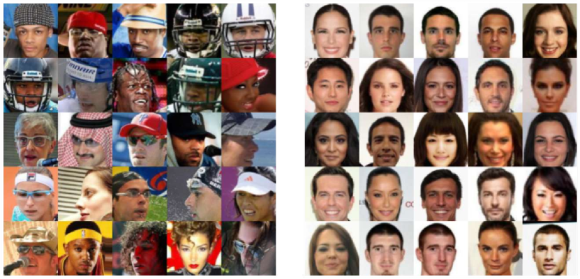
Figure 3: The most (and the least) unique CelebA real samples determined by our proposed metric, minority score. Samples with the highest (left) and the lowest (right) minority scores are exhibited.

3.2 Minority score: Measuring the uniqueness

Based on the intuitions that we gained in Section 3.1, we develop a metric for describing the uniqueness of features of given samples using diffusion models. We saw that the minority samples often lose significant amount of their perceptual information after going through the perturbation-reconstruction procedure. Hence, we employ the LPIPS distance (Zhang et al., 2018) between the original sample ${\boldsymbol{x}}_{0}$ and the restored version $\hat{{\boldsymbol{x}}}_{0}$, formally written as:

$$l({\boldsymbol{x}}_{0};{\boldsymbol{s}}_{\boldsymbol{\theta}})\coloneqq\mathbb{E}_{q_{\alpha_{t}}({\boldsymbol{x}}_{t}\mid{\boldsymbol{x}}_{0})}[d({\boldsymbol{x}}_{0},\hat{{\boldsymbol{x}}}_{0}({\boldsymbol{x}}_{t},{\boldsymbol{s}}_{\boldsymbol{\theta}}))],$$ (6)

where $d(\cdot,\cdot)$ denotes the LPIPS loss between two samples, and $t$ is a timestep used for perturbation; see Appendix B for details on our choice of $t$. The expectation is introduced for randomness due to the perturbation. We call this metric minority score, since it would yield high values for the minorities that contain novel attributes. Figure 3 visualizes the effectiveness of minority score specifically on the CelebA training samples. On the left side, we see samples that contain unique attributes like “Eyeglasses” and “Wearing_Hat” that are famously known as low-density features of the dataset (Amini et al., 2019; Yu et al., 2020). On the other hand, the samples on the right-side reveal features that look relatively common. We provide quantitative results that further validate the effectiveness of our metric in the next section; see Figure 8 for details.

Thanks to the one-shot characteristic offered by Tweedie’s formula, our minority score is efficient to compute when compared to the previous methods that rely upon iterative forward and reverse diffusion processes, hence requiring a number of evaluations of models (Wolleb et al., 2022; Wyatt et al., 2022; Teng et al., 2022). In contrast, our metric requires only a few number of function evaluations (even counting forward passes needed for LPIPS computations).

Remark 3.2 (The use of other distances in place of LPIPS).

One may wonder: why don’t we just use L1 or L2 distances for minority score, which are more accessible and efficient than the LPIPS metric? In fact, we observed that minority score can also work with such measures (to a certain extent), yielding some meaningful results in identifying minority-featured samples. However, they are sensitive to differences in some less-semantic information such as brightness and saturation in image data. So they tend to score high values not only to novel-featured samples, but also to ones that contain bright and highly-saturated visual aspects (which are often vanished during the perturbation-reconstruction process). See Figure 9 for instance. On the other hand, we did not observe such impurity in the LPIPS metric, and therefore stick to it in all our main implementation.

3.3 Minority guidance: Tackling the preference

Here a natural question arises. What can we do for tackling the inherent bias of diffusion models (to common attributes) using minority score at hand, so that they become more likely to generate the novel-featured samples? To address this question, we take a conditional generation approach where we incorporate minority score as a conditioning variable into the generation process, which can then serve to produce the unique-featured samples by conditioning w.r.t. high minority score values. Specifically to condition the existing framework with minimal effort, we employ the classifier guidance (Dhariwal & Nichol, 2021) that does not require re-building of class-conditional diffusion models. Below we describe in detail how we develop the conditional generation framework for minority score based on the classifier guidance technique.

Consider a dataset ${\boldsymbol{x}}_{0}^{(1)},\dots,{\boldsymbol{x}}_{0}^{(N)}\overset{\text{i.i.d.}}{\sim}q({\boldsymbol{x}}_{0})$ and a diffusion model ${\boldsymbol{s}}_{\boldsymbol{\theta}}({\boldsymbol{x}}_{t},t)$ (pre-trained on the dataset). For each sample, we compute minority score via (6) and obtain $l^{(1)},\dots,l^{(N)}$ where $l^{(i)}\coloneqq l({\boldsymbol{x}}_{0}^{(i)},{\boldsymbol{s}}_{\boldsymbol{\theta}}),i\in\{1,\dots,N\}$. We process the (positive-valued) minority scores as ordinal data with $L$ categories by thresholding them with $L-1$ levels of minority score. This yields the ordinally categorized minority scores $\tilde{l}^{(1)},\dots,\tilde{l}^{(N)}\in\{0,\dots,L-1\}$ where $\tilde{l}=0$ and $\tilde{l}=L-1$ indicate the classes w.r.t. the most common and the rarest features, respectively. The ordinal minority scores are then coupled with the associated data samples to yield a paired dataset $({\boldsymbol{x}}_{0}^{(1)},\tilde{l}^{(1)}),\dots,({\boldsymbol{x}}_{0}^{(N)},\tilde{l}^{(N)})$ which is subsequently used for training a (noise-conditioned) classifier $p_{\boldsymbol{\psi}}\big{(}\tilde{l}|{\boldsymbol{x}}_{t}\big{)}$ that predicts $\tilde{l}$ for input ${\boldsymbol{x}}_{t}$ (perturbed via (1)). After training, we blend the given score model with the log-gradient of the classifier as in (4) to yield a modified score:

$$\hat{{\boldsymbol{s}}}_{\boldsymbol{\theta}}\big{(}{\boldsymbol{x}}_{t},t,\tilde{l}\big{)}\coloneqq{\boldsymbol{s}}_{\boldsymbol{\theta}}({\boldsymbol{x}}_{t},t)+w\nabla_{{\boldsymbol{x}}_{t}}\log p_{\boldsymbol{\psi}}\big{(}\tilde{l}\mid{\boldsymbol{x}}_{t}\big{)},$$

where $\boldsymbol{\psi}$ indicates parameterization for the classifier, and $w$ is a scaling factor for the guidance; see Figure 5 for details on its impact. Incorporating this mixed score into the sampling process (3) then enables conditional generation w.r.t. $\hat{p}_{\boldsymbol{\theta}}({\boldsymbol{x}}_{t}|\tilde{l})\propto p_{\boldsymbol{\theta}}({\boldsymbol{x}}_{t})p_{\boldsymbol{\psi}}\big{(}\tilde{l}|{\boldsymbol{x}}_{t}\big{)}^{w}$. We call our technique minority guidance, as it gives guidance w.r.t. minority score in the generation process. Notice that generating unique-featured samples is now immediate, e.g., by conditioning an arbitrarily high $\tilde{l}$ via minority guidance. Even more, our sampler enables a free control of the uniqueness of features for generated samples (to the extent that a given pre-trained backbone model can represent), which has never been offered in literature so far to our best knowledge.

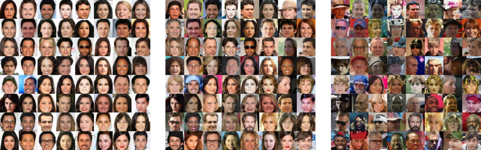
Figure 4: Generated samples from minority guidance over various minority classes $\tilde{l}$. The results are obtained on CelebA where the number of minority classes is $L=100$. Generated samples conditioned on $\tilde{l}=0$ (left), $\tilde{l}=50$ (middle), and $\tilde{l}=99$ (right) are exhibited. We share the same random seed for all three minority classes. The classifier scale is fixed as $w=2.0$.

Details on categorizing minority score. For the threshold levels to compart the (raw) minority scores (obtained via (6)), we observed that a naive equally-spaced thresholds yield significant imbalance in the size of classes (e.g., extremely small numbers of samples in highly unique classes), which would then yield negative impacts in the performance of the classifier especially against the small-sized classes. Hence, we resort to splitting the minority scores based on their quantiles. When $L=10$ for instance, we categorize the minority scores such that $\tilde{l}=9$ ($\tilde{l}=0$) becomes the samples with the top (bottom) $10\%$ of the uniquely-featured samples. For the number of classes $L$, using ones that yield benign numbers of samples per each class (e.g., over $100$ samples) being chosen based on the size of a given dataset usually offers good performances. See Figures 10 and 11 for demonstration. We also found that $L$ can serve as a control knob for balancing the faithfulness of the guidance with the controllability over the uniqueness of features. We leave a detailed discussion on this point in Section C.2.

4 Experiments

In this section, we provide empirical demonstrations that validate our proposals and arguments, specifically focusing on the unconditional image generation task. To this end, we first clarify the setup used in our demonstrations (see Appendix B for more details) and then provide results for the proposed approach in comparison with existing frameworks.

4.1 Setup

Datasets and pre-trained models. We consider three benchmark datasets: unconditional CIFAR-10 (Krizhevsky et al., 2009), CelebA $64\times 64$ (Liu et al., 2015), and LSUN-Bedrooms $256\times 256$ (Yu et al., 2015). For the unconditional CIFAR-10 model, we employ the checkpoint provided in Nichol & Dhariwal (2021). The pre-trained model for CelebA is constructed by ourselves via the architecture and setting used in Dhariwal & Nichol (2021). The backbone model for LSUN-Bedrooms is taken from Dhariwal & Nichol (2021).

Classifiers for minority guidance. We employ the encoder architecture of U-Net used in Dhariwal & Nichol (2021) for all of our guidance classifiers. For CIFAR-10 and CelebA results, we employ all training samples for constructing the minority classifiers (e.g., $N=50000$ for CIFAR-10). On the other hand, only a $10\%$ of the training samples are employed for building the minority classifier for the results on LSUN-Bedrooms. For the number of minority classes $L$, we take $L=100$ for all three datasets.

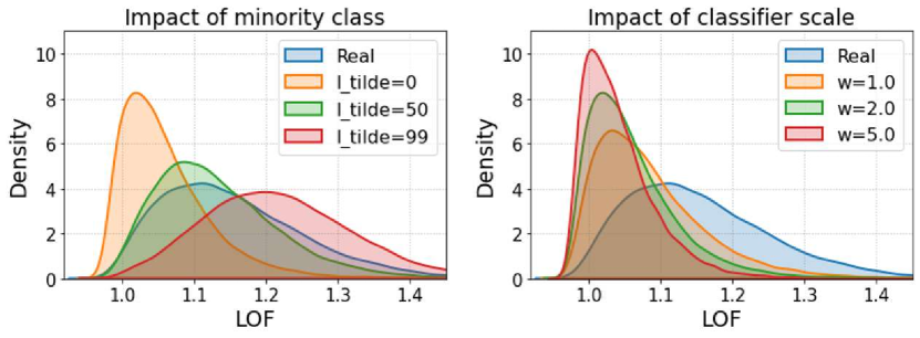
Figure 5: Impacts of minority class $\tilde{l}$ (left) and classifier scale $w$ (right) on the density of Local Outlier Factor (LOF) (Breunig et al., 2000) on CelebA. The higher LOF, the less likely (i.e., more unique-featured) samples. “Real” refers to the test set of CelebA. The other parameters are fixed: $w=2.0$ (left) and $\tilde{l}=0$ (right).

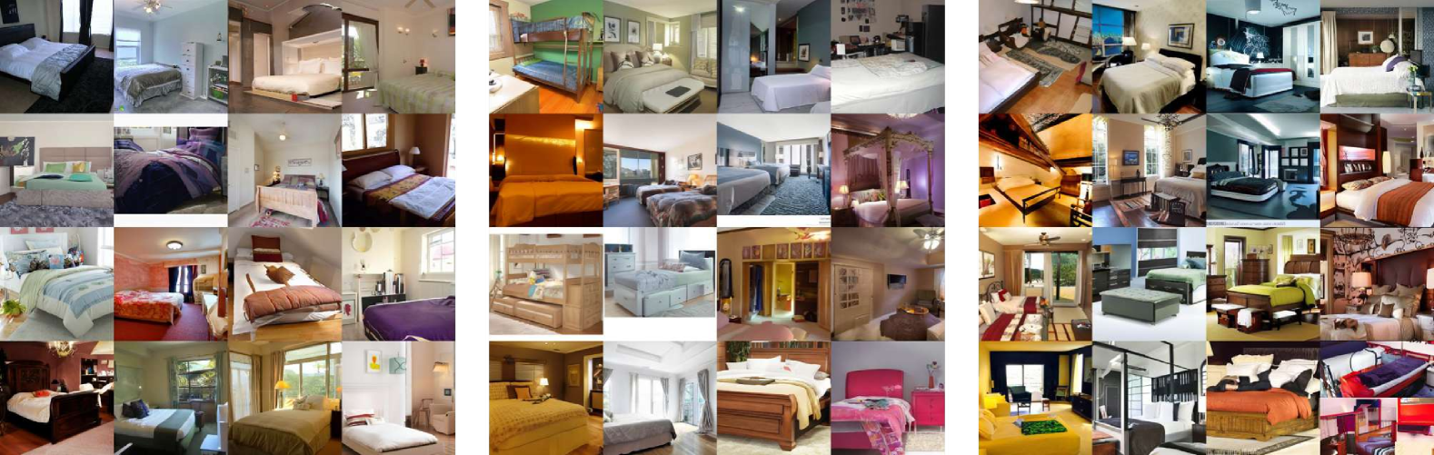
Figure 6: Sample comparison on LSUN-Bedrooms focused on the DDPM-based methods. See Figure 23 for comparison with samples from StyleGAN (Karras et al., 2019). Generated samples from ancestral sampling (Ho et al., 2020) (left), our method conditioned on majority (middle) and minority (right) classes are exhibited. We use the same random seed for all three cases.

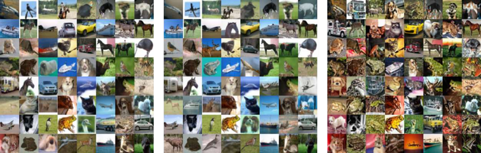
Figure 7: Sample comparison on unconditional CIFAR-10 considering the DDPM-based samplers. We leave comparison with BigGAN (Brock et al., 2019) in Figure 21. Generated samples from ancestral sampling (Ho et al., 2020) (left), the proposed sampler focused on majority (middle) and minority (right) classes are provided. We share the same random noise for all three settings.

Baselines. Since there has been lack of studies that explored the minority-focused generation in the unconditional setting as ours (see related work in Section 1 for details), we consider three generic frameworks that are widely adopted in literature. The first two baselines are GAN-based frameworks, BigGAN (Brock et al., 2019) and StyleGAN (Karras et al., 2019). The third baseline, which is our main interest for comparison, is a diffusion-based generative model, DDPM (Ho et al., 2020) with the standard sampler (3). The BigGAN models are employed for CIFAR-10 and CelebA, and built with the settings provided in the author’s official project page. We employ StyleGAN for LSUN-Bedrooms using the checkpoint provided in Karras et al. (2019). The DDPM baseline is compared in all three datasets and shares the same pre-trained models as ours. Additionally to comparison with the generative baselines, we also employ the ground-truth real data, especially in terms of neighborhood density (see below for details on the focused metrics).

Evaluation metrics. For the purpose of evaluating the generation capability of low-density samples, we focus on two well-known measures for describing the density of neighborhoods: Average k-Nearest Neighbor (AvgkNN) and Local Outlier Factor (LOF) (Breunig et al., 2000). AvgkNN measures density via proximity to k-nearest neighbors. On the other hand, LOF compares density around a given sample to density around its neighbors. For both measures, a higher value indicates that a given sample lies on a lower-density region compared to its neighboring samples (Sehwag et al., 2022). We evaluate the two metrics in the feature space of ResNet-50 (He et al., 2016) as in Sehwag et al. (2022). In addition to the twin neighborhood measures, we employ minority score to further augment our evaluation. The improved precision (Kynkäänniemi et al., 2019) is used for assessing sample quality. All measures are evaluated with 50K generated samples.

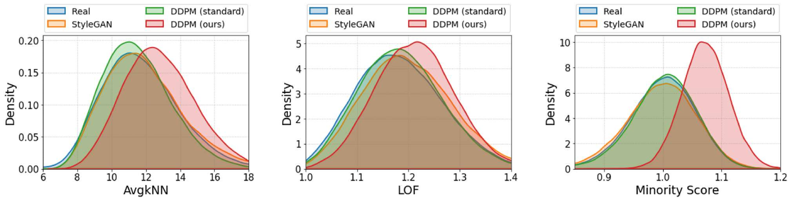
Figure 8: Comparison of neighborhood density on LSUN-Bedrooms. We found the same trends on the other two datasets and leave the results in Section D.3. “Real” refers to our real-data baseline, the training set of LSUN-Bedrooms. “StyleGAN” is one of our generative baselines, StyleGAN (Karras et al., 2019). “DDPM (standard)” indicates another generative baseline on the dataset: DDPM with the standard sampler (3) (Ho et al., 2020). “DDPM (ours)” denotes DDPM with the proposed sampler, minority guidance. “AvgkNN” refers to Average k-Nearest Neighbor, and “LOF” is Local Outlier Factor (Breunig et al., 2000). “Minority Score” corresponds to our proposed metric for describing the uniqueness of samples. The higher values, the less likely samples for all measures.

4.2 Results

Validation of the roles of $\tilde{l}$ and $w$. Figure 4 visualizes generated samples from minority guidance considering a variety of the (categorized) minority class $\tilde{l}$. The left figure corresponds to $\tilde{l}=0$, while the middle and the right figures are due to $\tilde{l}=50$ and $\tilde{l}=99$, respectively. We use the same random seed for generation of all three classes. Observe that as $\tilde{l}$ increases, the samples tend to have more rare features that appear similar to the ones observable in the minority samples (e.g., in Figure 3). The left plot of Figure 5 illustrates this impact in a quantitative manner. We see that increasing $\tilde{l}$ yields the LOF density shifting toward high-valued regions (i.e., low-density regions), which corroborates the observation made in Figure 4. On the other hand, the right plot of Figure 5 exhibits the impact of the classifier scale $w$. Notice that an increase in $w$ makes the LOF density squeezing toward low-valued regions (i.e., high-probability regions). This aligns with the well-known role of $w$ (see Section 2.2 for details) that determines whether to focus on some prominent attributes for the conditioned class (Dhariwal & Nichol, 2021). See Figure 18 for generated samples that visualize this impact.

Comparison with the baselines. Figure 6 visualizes generated samples on LSUN-Bedrooms considering the DDPM-based sampling methods. From left to right, the figures correspond to samples from ancestral sampling (Ho et al., 2020), our method conditioned on majority and minority classes, respectively. For all three cases, we share the same random seed for generating noise. Observe that our minority guidance, when focused on a novel-featured class, produces more exquisite and unique images compared to the standard sampler. Notably, it often encourages some monotonous-looking features (due to the standard method) to be more novel, e.g., with inclusions of additional objects like lamps. We found that such sophisticated attributes are in fact novel features that yield high minority score values in LSUN-Bedrooms; see Figure 16 for details. Figure 7 exhibits generated samples on unconditional CIFAR-10 w.r.t. the DDPM-based samplers. The left figure exhibits samples from ancestral sampling, and the middle (right) figure is due to ours focused on a majority (minority) class, respectively. Again, we share the same random noise for all three cases. We see the same trends on the performance benefits of ours relative to the baseline sampler; see Figure 17 for visualization of unique features in CIFAR-10.

Figure 8 provides performance comparison of neighborhood density measures on LSUN-Bedrooms. Observe that minority guidance outperforms the baselines in generating low-density unique samples for all three measures. Also notice that minority score exhibits a similar trend as the other measures, demonstrating its effectiveness as a metric for minority description. Table 1 exhibits sample quality of the considered methods. We observe that when focused on unique features, samples from minority guidance exhibit degraded fidelity. We conjecture that such degradation is attributed to limited knowledge of the backbone models on the unique features due to their extremely small volume in training data. This is supported by our results w.r.t. majority features that yield superior sample quality compared to the baselines; see Table 1 for instance. We leave a detailed analysis on this point in Section C.5.

	Precision
Method	CIFAR-10	CelebA	LSUN
BigGAN	0.8250	0.8593	–
StyleGAN	–	–	0.7310
DDPM (standard)	0.8795	0.8714	0.7686
DDPM (ours-minor)	0.7581	0.7951	0.5935
DDPM (ours-major)	0.8979	0.9123	0.7895

Table 1: Comparison of sample quality. “DDPM (ours-minor)” is minority guidance focused on minority features (e.g., $\tilde{l}=99$). “DDPM (ours-major)” also indicates the proposed sampler yet configured for minority classes (e.g., $\tilde{l}=50$). We mark the best result in bold and the second-best with underline.

5 Conclusion and Limitations

We showed that the conventional DSM-based diffusion models are inherently biased to produce high-likelihood majority samples. In light of this, we introduced a novel metric to evaluate the uniqueness of features and developed a sampling technique that can serve to generate novel-featured minority samples. We demonstrated that the proposed sampler greatly improves the capability of producing the low-density minority samples over existing generative methods. We believe that this is an important step toward fairness in generative models, with the goal of preventing discrimination caused by model and data biases.

One disadvantage is that the quality of minority samples due to our framework is predominantly determined by the knowledge of a given pre-trained model, which is often limited w.r.t. minor features that are rarely seen during training. Another flip side is that our approach requires access to a good number of real samples (while being unlabeled), which may not be feasible in some highly limited situations. Hence, we believe one promising future direction is to push the boundary towards such challenging scenarios while addressing the limited knowledge issue.

Appendix A Proof of Proposition 3.1

Proposition 3.1.

Consider the DSM optimization in (2). Assume that a given noise-conditioned score network ${\boldsymbol{s}}_{\boldsymbol{\theta}}({\boldsymbol{x}}_{t},t)$ have enough capacity. Then for each timestep $t$, the optimality of the score network is achievable at:

$${\boldsymbol{s}}^{*}_{\boldsymbol{\theta}}({\boldsymbol{x}}_{t},t)=\mathbb{E}_{q({\boldsymbol{x}}_{0}\mid{\boldsymbol{x}}_{t})}\left[\nabla_{{\boldsymbol{x}}_{t}}\log{q_{\alpha_{t}}({\boldsymbol{x}}_{t}\mid{\boldsymbol{x}}_{0})}\right].$$

Proof.

Since the score network ${\boldsymbol{s}}_{\boldsymbol{\theta}}({\boldsymbol{x}}_{t},t)$ is assumed to be large enough, it can achieve the global optimum that minimizes the DSM objectives for all timesteps regardless of their weights in (2) (Song et al., 2020a). Hence, we can safely ignore the weighted sum and focus on the DSM objective for a specific timestep $t$ to derive ${\boldsymbol{s}}^{*}_{\boldsymbol{\theta}}({\boldsymbol{x}}_{t},t)$:

$${\boldsymbol{s}}^{*}_{\boldsymbol{\theta}}({\boldsymbol{x}}_{t},t)=\arg\min_{{\boldsymbol{s}}_{\boldsymbol{\theta}}\in\mathcal{S}}\mathbb{E}_{q({\boldsymbol{x}}_{0})q_{\alpha_{t}}({\boldsymbol{x}}_{t}\mid{\boldsymbol{x}}_{0})}[\|{\boldsymbol{s}}_{\boldsymbol{\theta}}({\boldsymbol{x}}_{t},t)-\nabla_{{\boldsymbol{x}}_{t}}\log q_{\alpha_{t}}({\boldsymbol{x}}_{t}\mid{\boldsymbol{x}}_{0})\|_{2}^{2}],$$ (7)

where we consider the optimization over function space ${\boldsymbol{s}}_{\boldsymbol{\theta}}\in\mathcal{S}$ instead of the parameter space ${\boldsymbol{\theta}}\in\Theta$ for the ease of analysis. The objective function in (7) can be rewritten as:

$$\mathbb{E}_{q({\boldsymbol{x}}_{0})q_{\alpha_{t}}({\boldsymbol{x}}_{t}\mid{\boldsymbol{x}}_{0})}[\|{\boldsymbol{s}}_{\boldsymbol{\theta}}({\boldsymbol{x}}_{t},t)-\nabla_{{\boldsymbol{x}}_{t}}\log q_{\alpha_{t}}({\boldsymbol{x}}_{t}\mid{\boldsymbol{x}}_{0})\|_{2}^{2}]$$

$$= \int\int q({\boldsymbol{x}}_{0})q_{\alpha_{t}}({\boldsymbol{x}}_{t}\mid{\boldsymbol{x}}_{0})\|{\boldsymbol{s}}_{\boldsymbol{\theta}}({\boldsymbol{x}}_{t},t)-\nabla_{{\boldsymbol{x}}_{t}}\log q_{\alpha_{t}}({\boldsymbol{x}}_{t}\mid{\boldsymbol{x}}_{0})\|_{2}^{2}\;\;d{\boldsymbol{x}}_{t}\;d{\boldsymbol{x}}_{0}$$

$$= \int\underbrace{\int q_{\alpha_{t}}({{\boldsymbol{x}}_{t}})q({\boldsymbol{x}}_{0}\mid{\boldsymbol{x}}_{t})\|{\boldsymbol{s}}_{\boldsymbol{\theta}}({\boldsymbol{x}}_{t},t)-\nabla_{{\boldsymbol{x}}_{t}}\log q_{\alpha_{t}}({\boldsymbol{x}}_{t}\mid{\boldsymbol{x}}_{0})\|_{2}^{2}\;\;d{\boldsymbol{x}}_{0}}_{\eqqcolon{\cal L}({\boldsymbol{s}}_{\boldsymbol{\theta}},{\boldsymbol{x}}_{t})}\;d{\boldsymbol{x}}_{t}.$$

Since the objective function in (7) is a functional and convex w.r.t. ${\boldsymbol{s}}_{\boldsymbol{\theta}}$, we can apply the Euler-Lagrange equation (Gelfand et al., 2000) to come up with a condition for the optimality:

$$\frac{\partial{\cal L}}{\partial{\boldsymbol{s}}_{\boldsymbol{\theta}}}=0\;\;\Rightarrow\;\;\int q_{\alpha_{t}}({\boldsymbol{x}}_{t})q({\boldsymbol{x}}_{0}\mid{\boldsymbol{x}}_{t})\cdot 2\left\{{\boldsymbol{s}}^{*}_{\boldsymbol{\theta}}({\boldsymbol{x}}_{t},t)-\nabla_{{\boldsymbol{x}}_{t}}\log q_{\alpha_{t}}({\boldsymbol{x}}_{t}\mid{\boldsymbol{x}}_{0})\right\}\;d{\boldsymbol{x}}_{0}=0.$$

Rearranging the RHS of the arrow gives:

$$\int q_{\alpha_{t}}({\boldsymbol{x}}_{t})q({\boldsymbol{x}}_{0}\mid{\boldsymbol{x}}_{t})\cdot 2\left\{{\boldsymbol{s}}^{*}_{\boldsymbol{\theta}}({\boldsymbol{x}}_{t},t)-\nabla_{{\boldsymbol{x}}_{t}}\log q_{\alpha_{t}}({\boldsymbol{x}}_{t}\mid{\boldsymbol{x}}_{0})\right\}\;d{\boldsymbol{x}}_{0}=0$$

$$\Rightarrow \;\;{\boldsymbol{s}}^{*}_{\boldsymbol{\theta}}({\boldsymbol{x}}_{t},t)\int q({\boldsymbol{x}}_{0}\mid{\boldsymbol{x}}_{t})\;d{\boldsymbol{x}}_{0}=\int q({\boldsymbol{x}}_{0}\mid{\boldsymbol{x}}_{t})\nabla_{{\boldsymbol{x}}_{t}}\log q_{\alpha_{t}}({\boldsymbol{x}}_{t}\mid{\boldsymbol{x}}_{0})\;d{\boldsymbol{x}}_{0}$$

$$\Rightarrow \;\;{\boldsymbol{s}}^{*}_{\boldsymbol{\theta}}({\boldsymbol{x}}_{t},t)=\mathbb{E}_{q({\boldsymbol{x}}_{0}\mid{\boldsymbol{x}}_{t})}\left[\nabla_{{\boldsymbol{x}}_{t}}\log{q_{\alpha_{t}}({\boldsymbol{x}}_{t}\mid{\boldsymbol{x}}_{0})}\right].$$

This completes the proof. ∎

Appendix B Additional Details on Experimental Setup

For the unconditional CIFAR-10 model, we employ the checkpoint provided in Nichol & Dhariwal (2021) without fine-tuning or modification. The pre-trained model for the CelebA results is based upon the architecture used in Dhariwal & Nichol (2021) for ImageNet $64\times 64$, and trained with the setting used in Nichol & Dhariwal (2021) for unconditional ImageNet $64\times 64$. The backbone model for LSUN-Bedrooms was taken from Dhariwal & Nichol (2021) and used without modifications. For the results on LSUN Bedrooms, a $10\%$ of the training samples provided in a publicly available Kaggle repository are employed for building the minority classifier. The BigGAN model for the CIFAR-10 experiments are trained with the setting provided in the author’s official project page. For the CelebA model, we respect the architecture used in Choi et al. (2020) and follow the same training setup as the CIFAR-10 model. We employ StyleGAN for LSUN-Bedrooms using the checkpoint provided in Karras et al. (2019). The DDPM baseline shares the same pre-trained models as ours. We employ the implementation from PyOD (Zhao et al., 2019) to compute our twin neighborhood measures, Average k-Nearest Neighbor (AvgkNN) and Local Outlier Factor (LOF). We respect the conventional choices for the numbers of nearest neighbors for computing the measures: $5$ (AvgkNN) and $20$ (LOF). We employ $k=5$ for evaluating precision.

For the perturbation timestep used for computing minority score (i.e., $t$ in (6)), we employ $t=0.9T$ in all settings where $T$ indicates the total number of steps that a given backbone model is trained with. For instance, we use $t=3600$ for unconditional CIFAR-10 where the pre-trained model is configured with $T=4000$. We employ 250 timesteps to sample from the baseline DDPM for all its results. For our minority guidance, the same 250 timesteps are mostly employed, yet we occasionally use 100 timesteps for speeding-up sampling (e.g., when conducting ablation studies), since we found that it yields little degradation as reported in Dhariwal & Nichol (2021). Our implementation is based on PyTorch (Paszke et al., 2019), and all experiments are performed on twin A100 GPUs. See the attached supplementary zip file for code.

Appendix C Ablation Studies, Analyses, and Discussions

We continue from Sections 3 and 4 of the main paper and provide ablation studies and discussions on the proposed approach. We first consider the use of other distance metrics for minority score in place of LPIPS. After that, we ablate the number of classes $L$ and investigate its impact on the performance of minority guidance. We also explore the sensitiveness of our algorithm w.r.t. the number of available samples $N$. We then investigate another strategy for the minority-focused generation, which is naturally given by our minority score. Lastly, we give an analysis to provide a rationale on quality degradation observed in samples from minority guidance when specifically focusing on minority classes.

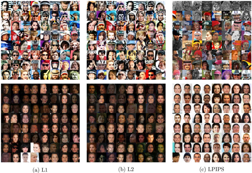
Figure 9: Performance comparison of minority score with various distance metrics. The most novel (top row) and the most common (bottom row) CelebA real training samples determined by minority scores based on (a) L1; (b) L2; and (c) LPIPS (our proposal) are exhibited.

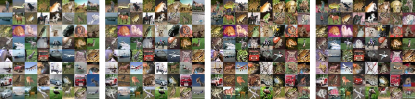
Figure 10: Sample comparison on unconditional CIFAR-10 considering a range of minority classes $L$ for our approach. We share the same random seed for generating all four groups of samples: (i) DDPM with ancestral sampling (leftmost); (ii) ours with $L=10$ (middle-left); (iii) ours with $L=100$ (middle-right); (iv) ours with $L=1000$ (rightmost). All generations from our approach focus on the most unique classes under its own setting (e.g., $\tilde{l}=999$ for $L=1000$). The classifier scale is fixed as $w=3.0$.

C.1 The distance metric for minority score

Figure 9 compares the performances of several versions of minority score employing distinct distance metrics. We see that samples containing bright and highly-saturated visual aspects score high values from the L1 and L2 versions. This implies that such variated minority scores are sensitive to less-semantic information like brightness and saturation (as noted in Remark 3.2). On the other hand, we observe that the original version using LPIPS does not exhibit such sensitiveness, yielding results being disentangled with brightness and saturation of samples. Furthermore, it succeeds in identifying some weird-looking abnormal samples latent in the dataset (see the samples in the first row of the right column) while the other versions fail to find them due to their distraction, e.g., to bright and highly-saturated instances.

C.2 The number of classes $L$ for minority guidance

We first discuss how the number of classes $L$ can be used for balancing between the faithfulness of the guidance and the controllability over the uniqueness of features. We then provide an empirical study that ablates the number of classes $L$ and explores its impact on the performance of minority guidance.

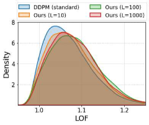
Figure 11: Impact of the number of minority classes $L$ on the density of Local Outlier Factor (LOF) (Breunig et al., 2000). The results are obtained on unconditional CIFAR-10. The higher LOF, the less likely samples. All the settings and baseline are the same as those in Figure 13.

Consider a case where we use a small $L$ for constructing ordinal minority scores. This leads to large numbers of samples per class and therefore helps to build a faithful classifier that well captures class-wise representations. However, if we use too small $L$, then it induces samples containing wide variety of features being flocked into small categorical ranges, thus making it difficult to produce them separately (i.e., losing the controllability). One extreme case that helps understand this is when $L=1$, where the sampler then becomes just the standard one (3) where we don’t have any control over the uniqueness of features. On the other hand, employing large $L$ would make the generation highly controllable w.r.t. the uniqueness of features. However, too large $L$ results in vast numbers of small-sized classes, which makes the classifier hard to capture class-wise representations properly, thereby resulting in a crude predictor that rarely gives meaningful guidance. Considering the other extreme case $L=N$ where the number of classes is the same as the number of samples, the classifier therein would never be able to learn representations over classes well enough for making meaningful guidance for the uniqueness of features. Therefore, we can say that it is important to set a proper $L$ that well balances between the controllability and the faithfulness. Nonetheless, we empirically observed that our minority guidance is robust to the choice of $L$, and a properly selected (yet not that difficult to come up with) $L$ yielding benign numbers of samples for each classes (e.g., containing over $100$ samples per class) performs well regardless of $L$, i.e., effectively producing samples with desired features while maintaining realistic sample quality. Below we provide demonstrations that validate the above descriptions.

Figure 10 exhibits generated samples concerning a variety of minority classes $L$, and Figure 11 provides a quantitative version of the results under the same settings. Observe that for all considered $L$, our approach improves generative capability of the minority samples over the baseline DDPM sampler, which demonstrates its robustness w.r.t. the number of minority classes $L$. However, we note that $L=100$ offers better guidance for the minority features than $L=1000$, yielding a more tilted LOF density toward minority regions (i.e., high LOF values). This validates the role of $L$ as a balancing knob for the faithfulness of the guidance and the controllability over the uniqueness.

C.3 The number of available samples $N$

Method	Recall
Ours (all)	0.7736
Ours (20%)	0.6829

Table 2: Impact of $N$ on sample diversity. The results are obtained on unconditional CIFAR-10.

Figure 12 and Table 2 provide empirical results that ablate the number of available samples $N$ specifically on unconditional CIFAR-10. Observe that even with limited numbers of samples that are much smaller than the full training set, minority guidance still offers significant improvement in the minority-focused generation over the baseline DDPM sampler. In fact, this benefit is already demonstrated via our experiments on LSUN-Bedrooms presented in Section 4.2 where we only take a $10\%$ of the total training set in obtaining great improvement; see Figures 6 and 8 therein. However, we see degraded diversity compared to the full dataset case, which is reflected in a lower recall (Kynkäänniemi et al., 2019) value; see Table 2 for details.

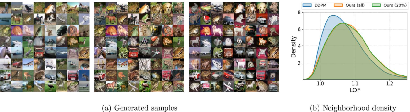
Figure 12: Experimental results that ablate the number of available samples $N$ for minority guidance. All results are obtained on unconditional CIFAR-10. (a) Generated samples from DDPM with ancestral sampling (left), ours with all training samples of CIFAR-10 (middle), and ours employing a 20% of training samples (right) are exhibited. We use the same random seed for all three settings; (b) Impact of $N$ on our neighborhood density measure, the density of Local Outlier Factor (LOF) (Breunig et al., 2000). The higher LOF, the less likely samples. All the settings and baseline are the same as those in (a).

C.4 Generation from $\hat{q}({\boldsymbol{x}}_{0})\propto q({\boldsymbol{x}_{0}})l({\boldsymbol{x}}_{0};{\boldsymbol{s}}_{\boldsymbol{\theta}})$

Recall our setting considered in Section 3.3 where we have a dataset ${\boldsymbol{x}}_{0}^{(1)},\dots,{\boldsymbol{x}}_{0}^{(N)}\overset{\text{i.i.d.}}{\sim}q({\boldsymbol{x}}_{0})$, a pre-trained diffusion model ${\boldsymbol{s}}_{\boldsymbol{\theta}}({\boldsymbol{x}}_{t},t)$, and minority score values associated with the dataset $l^{(1)},\dots,l^{(N)}$ where $l^{(i)}\coloneqq l({\boldsymbol{x}}_{0}^{(i)},{\boldsymbol{s}}_{\boldsymbol{\theta}}),i\in\{1,\dots,N\}$. Since our interest is to make samples with high $l^{(i)}$ (i.e., minority instances) more likely to be produced, one can naturally think of sampling from a blended distribution $\hat{q}({\boldsymbol{x}}_{0})\propto q({\boldsymbol{x}_{0}})l({\boldsymbol{x}}_{0};{\boldsymbol{s}}_{\boldsymbol{\theta}})$. However, simulating the generation process w.r.t. this mixed distribution is not that straightforward, since we do not have access to the score functions of its perturbed versions $\{\nabla_{{\boldsymbol{x}}_{t}}\log\hat{q}_{\alpha_{t}}({\boldsymbol{x}}_{t})\}_{t=1}^{T}$ where $\hat{q}_{\alpha_{t}}({\boldsymbol{x}}_{t})\coloneqq\int\hat{q}({\boldsymbol{x}}_{0})q_{\alpha_{t}}({\boldsymbol{x}}_{t}|{\boldsymbol{x}}_{0})d{\boldsymbol{x}}_{0}$.

To circumvent the issue, we take an approximated approach for obtaining the perturbed mixtures. Specifically, we first invoke another definition of the perturbed distributions $\hat{q}_{\alpha_{t}}({\boldsymbol{x}}_{t})\propto q_{\alpha_{t}}({\boldsymbol{x}_{t}})l({\boldsymbol{x}}_{t})$ where $l({\boldsymbol{x}}_{t})$ denotes minority score w.r.t. a noised instance ${\boldsymbol{x}}_{t}$ (describing the uniqueness of ${\boldsymbol{x}}_{t}$). This gives $\nabla_{{\boldsymbol{x}}_{t}}\log\hat{q}_{\alpha_{t}}({\boldsymbol{x}}_{t})={\boldsymbol{s}}_{\boldsymbol{\theta}}({\boldsymbol{x}}_{t},t)+\nabla_{{\boldsymbol{x}}_{t}}\log l({\boldsymbol{x}}_{t})$. Since $l({\boldsymbol{x}}_{t})$ is intractable, we resort to considering an approximated version $\hat{l}({\boldsymbol{x}}_{t})$ by computing an empirical average via the use of the minority classifier $p_{\boldsymbol{\psi}}(\tilde{l}|{\boldsymbol{x}}_{t})$:

$$\hat{l}({\boldsymbol{x}}_{t})\coloneqq\sum_{i=0}^{L-1}\tau_{i}\cdot p_{\boldsymbol{\psi}}(\tilde{l}=i\mid{\boldsymbol{x}}_{t}),$$

where $\{\tau_{i}\}_{i=0}^{L-1}$ denote the threshold levels used for categorizing minority score (see Section 3.3 for details). The score function of the perturbed mixture at timestep $t$ then reads:

$$\nabla_{{\boldsymbol{x}}_{t}}\log\hat{q}_{\alpha_{t}}({\boldsymbol{x}}_{t})\approx{\boldsymbol{s}}_{\boldsymbol{\theta}}({\boldsymbol{x}}_{t},t)+w\nabla_{{\boldsymbol{x}}_{t}}\log\hat{l}({\boldsymbol{x}}_{t}),$$ (8)

where $w$ is a parameter introduced for controlling the intensity of the mixing; see Figures 13 and 14 for demonstrations of its impact. We found that using the mixed score as a drop in replacement of ${\boldsymbol{s}}_{\boldsymbol{\theta}}({\boldsymbol{x}}_{t},t)$ in the standard sampler (3) improves the capability of diffusion models to generate low-density minority samples. Below we provide some empirical results that demonstrate its effectiveness.

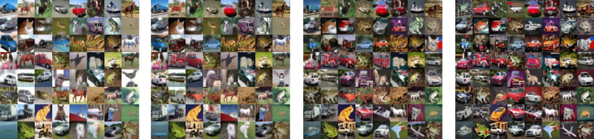
Figure 13: Generated samples using the approximated mixture score (8) over various intensity $w$. The results are obtained on unconditional CIFAR-10. We share the same random seed for all four cases: (i) $w=0.0$ (leftmost); (ii) $w=5.0$ (middle-left); (iii) $w=20.0$ (middle-right); (iv) $w=50.0$ (rightmost).

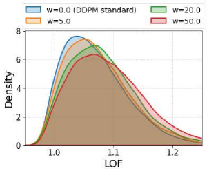
Figure 14: Impact of the mixing intensity $w$ on the density of LOF. The results are obtained on unconditional CIFAR-10.

Figure 13 visualizes generated samples via (8) concerning a variety of the blending intensity $w$. We use the same random seed for generation of all four settings. Observe that as $w$ increases, the samples become more likely to contain novel features w.r.t. the dataset (e.g., see Figure 17 for visualization of the unique features on CIFAR-10). This implies that $w$ plays a similar role as $\tilde{l}$ in minority guidance and therefore can be used for improving the generation capability for minority features. Figure 14 reveals the impact of $w$ in a quantitative manner. Notice that increasing $w$ yields the LOF density shifting toward high-valued regions (i.e., low-density regions), which corroborates the results shown in Figure 13 and further validates the role of $w$ as a knob for controlling whether to focus on the minority features.

While this alternative sampler based on the mixed distribution $\hat{q}({\boldsymbol{x}}_{0})\propto q({\boldsymbol{x}_{0}})l({\boldsymbol{x}}_{0};{\boldsymbol{s}}_{\boldsymbol{\theta}})$ yields significant improvement over the standard DDPM sampler (i.e., $w=0.0$ case), minority guidance still offers better controllability over the uniqueness of features thanks to the collaborative twin knobs $\tilde{l}$ and $w$. Hence, we adopt it as our main gear for tackling the preference of the diffusion models w.r.t. majority features.

C.5 Limited knowledge of pre-trained models on minorities

We hereby provide an inspection of our pre-trained models on whether they faithfully capture the minority features, specifically focusing on the model used for the CelebA results. To this end, we first visualize some minority samples produced by the backbone model and examine if some weird-looking visual aspects are seen. Also, we provide quantitative results for a more precise assessment of the model’s knowledge on the unique features.

Figure 15 exhibits a number of unique-featured samples drawn from the pre-trained DDPM model. The samples presented herein are the ones that yield the highest minority scores among 50K generated samples via ancestral sampling (Ho et al., 2020). We observe some unrealistic instances in the figure; see the left-most samples in the first row for instance. This implies that the knowledge of our pre-trained model on the minority features is actually limited, and therefore a faithful guidance that points to the minority features in a precise manner (like ours) may fail to produce realistic samples due to such limited representation inside the backbone.

Method	Precision
DDPM-standard	0.859
DDPM-minor	0.682
Ours-minor	0.789

Table 3: Sample quality of minority samples drawn from the pre-trained DDPM model on CelebA. “DDPM-minor” denotes the case w.r.t. the minority samples selected from the baseline DDPM (based on minority score).

Table 3 further strengthen our finding by giving quantitative results (w.r.t. the CelebA model). Specifically to focus on the quality of the minor samples that are rarely produced by the baseline sampler, we measure precision of the top-1K instances yielding the highest minority scores selected from the 50K samples generated by the pre-trained model (via ancestral sampling). For all computations, we employ 50K real samples (instead of 1K samples) to facilitate a more precise estimation of the real-data manifold. The fidelity w.r.t. the compared samples are evaluated in the same way (i.e., using 1K generated samples); see Table 1 for their precise (yet not that different from the values in Table 3, so validating our analysis made herein) performances. Notice in Table 3 that the fidelity of the selected 1K minority samples from the backbone model is in fact worse than the quality of less-unique samples (w.r.t. the same backbone model) as well as that of our minority guidance, reflected in lower precision of “DDPM-minor”. This corroborates our observation made upon Figure 15 and further demonstrates the lack of knowledge of the backbone model w.r.t. the minority attributes.

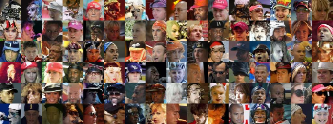
Figure 15: Unique-featured samples generated from the pre-trained model used for our CelebA experiments. The baseline DDPM sampler (Ho et al., 2020) is used for generation. The instances with the highest minority scores among 50K generated samples are exhibited.

Appendix D Additional Experimental Results

We continue from Section 4.2 of the main paper and provide some additional results. We first present visualizations of the unique and common features in CIFAR-10 and LSUN-Bedrooms. We then exhibit generated samples that visualize the impact of $w$. Also, we provide the complete results on all three datasets where we compare ours with the baselines in a thorough manner.

D.1 How do the unique features in CIFAR-10 and LSUN-Bedrooms look like?

Figure 16 exhibits the most unique (top) and common (bottom) features in LSUN-Bedrooms determined by minority score. Notice that the minority features presented herein share similar aspects as the ones from the generated samples from minority guidance exhibited in our main paper; see the right figure in Figure 6 for details. On the other hand, Figure 17 visualizes the same pair yet w.r.t. CIFAR-10. Again, we see the same unique attributes that we saw in our generated samples in the manuscript. See Figure 7 therein.

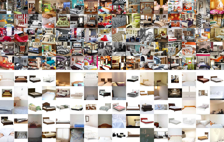
Figure 16: The most unique (top) and common (bottom) featured samples in LSUN-Bedrooms determined by minority score.

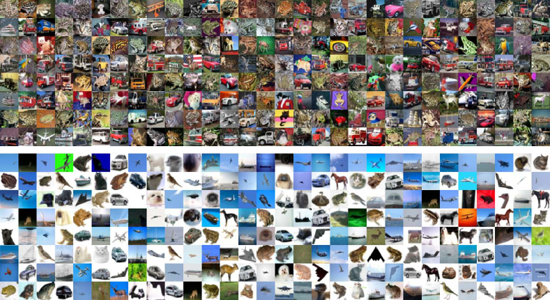
Figure 17: The most unique (top) and common (bottom) featured samples in the CIFAR-10 training set determined by minority score.

D.2 Visualization of the impact of $w$

Figure 18 provides generated samples that reveal the impact of the classifier scale $w$ of minority guidance (see the right plot in Figure 5 for a quantitative version of the result). We observe that as $w$ increase, the samples get more focused on prominent features that are representative in the corresponding class, e.g., staring straight ahead in the focused common class. This well aligns with the quantitative result shown in Figure 5, as well as the impact of $w$ that is well investigated in Dhariwal & Nichol (2021).

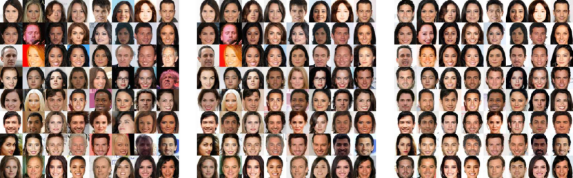
Figure 18: Generated samples from minority guidance over various classifier scale $w$. The results are obtained on CelebA. The class is fixed to the most common one (i.e., $\tilde{l}=0$). Generated samples with $w=1.0$ (left), $w=2.0$ (middle), and $w=5.0$ (right) are shown. We share the same random seed for all three settings.

D.3 Comparison with the baselines: Complete results

Figure 19 visualizes generated samples on CelebA for all considered methods. Observe that our minority guidance focused on a novel-featured class (i.e., the figure on the bottom-right) yields samples featured with ones that look similar to the low-density minority attributes exhibited in Figure 3 (as well as in the top-right figure in Figure 9). Figure 20 gives a quantitative validation to this observation, where we see minority guidance outperforms the other baselines in generating the low-density samples that score high-valued neighborhood measures. The same trend is observed in our CIFAR-10 results; see Figures 21 and 22 for details. For LSUN-Bedrooms, we provide sample comparison in Figure 23 where all the baselines including StyleGAN (Karras et al., 2019) are taken into account. See Figure 8 for the results on the neighborhood density measures.

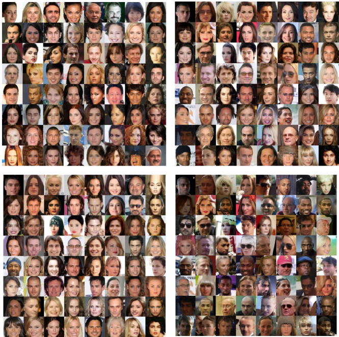
Figure 19: Sample comparison on CelebA considering all the baselines. Generated samples from BigGAN (Brock et al., 2019) (top-left), DDPM with ancestral sampling (Ho et al., 2020) (top-right), the proposed sampler focused on majority (bottom-left) and minority (bottom-right) classes are provided. We share the same random noise for generation based on the DDPM-based samplers.

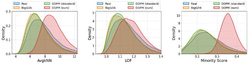
Figure 20: Comparison of neighborhood density on CelebA. “Real” refers to our real-data baseline, the test samples of CelebA. “BigGAN” is our GAN-based generative baseline, BigGAN (Brock et al., 2019). “DDPM (standard)” indicates another the diffusion-based generative baseline: DDPM with the standard sampler (3) (Ho et al., 2020). “DDPM (ours)” denotes DDPM with the proposed sampler, minority guidance. “AvgkNN” refers to Average k-Nearest Neighbor, and “LOF” is Local Outlier Factor (Breunig et al., 2000). “Minority Score” corresponds to our proposed metric for describing the uniqueness of samples. The higher values, the less likely samples for all measures.

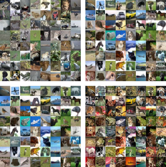
Figure 21: Sample comparison on unconditional CIFAR-10 considering all the baselines. Generated samples from BigGAN (Brock et al., 2019) (top-left), DDPM with ancestral sampling (Ho et al., 2020) (top-right), the proposed sampler focused on majority (bottom-left) and minority (bottom-right) classes are provided. We share the same random noise for generation based on the DDPM-based samplers.

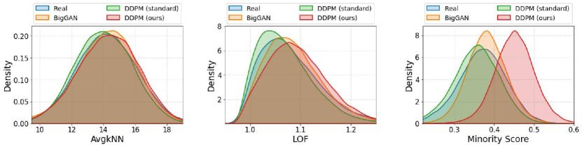
Figure 22: Comparison of neighborhood density on unconditional CIFAR-10. “Real” refers to our real-data baseline, the test samples of CIFAR-10. All the remaining settings are the same as those in Figure 20.

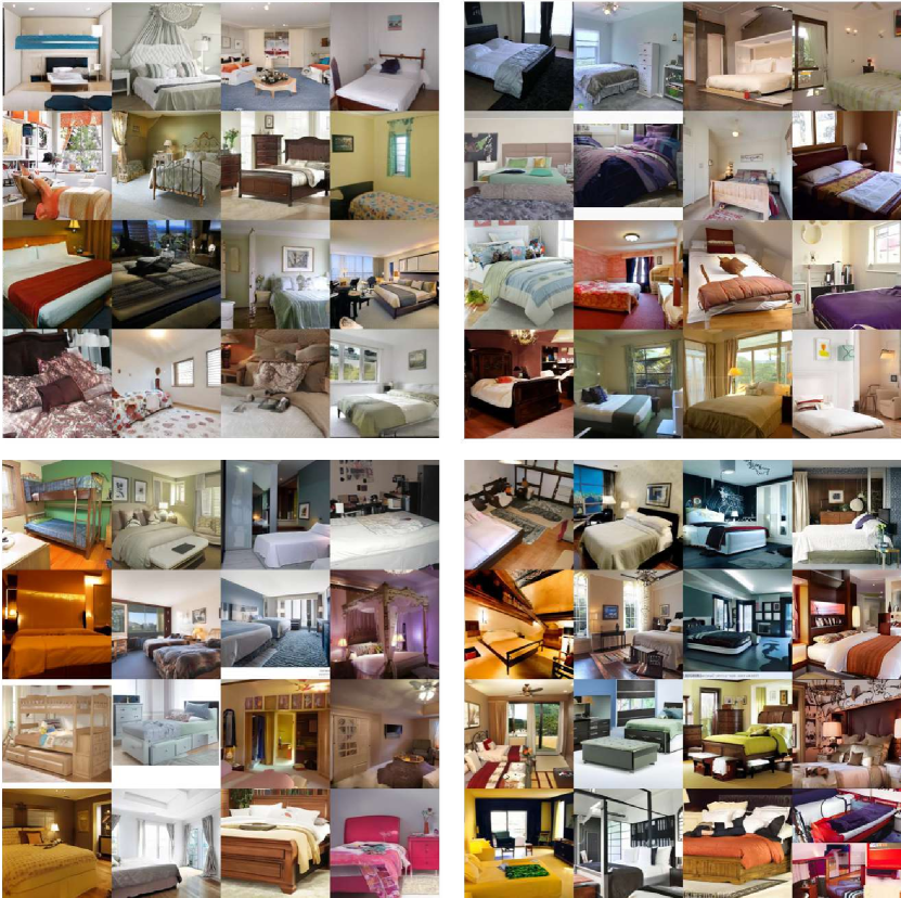
Figure 23: Sample comparison on LSUN-Bedrooms with all baseline methods. Generated samples from StyleGAN (Karras et al., 2019) (top-left), DDPM with ancestral sampling (Ho et al., 2020) (top-right), our method conditioned on majority (bottom-left) and minority (bottom-right) classes are exhibited. We share the same seed for generation w.r.t. the DDPM-based samplers.

References

- Agarwal et al. (2022) Agarwal, C., D’souza, D., and Hooker, S. Estimating example difficulty using variance of gradients. In Proceedings of the IEEE/CVF Conference on Computer Vision and Pattern Recognition, pp. 10368–10378, 2022.
- Amini et al. (2019) Amini, A., Soleimany, A. P., Schwarting, W., Bhatia, S. N., and Rus, D. Uncovering and mitigating algorithmic bias through learned latent structure. In Proceedings of the 2019 AAAI/ACM Conference on AI, Ethics, and Society, pp. 289–295, 2019.
- Breunig et al. (2000) Breunig, M. M., Kriegel, H.-P., Ng, R. T., and Sander, J. Lof: identifying density-based local outliers. In Proceedings of the 2000 ACM SIGMOD international conference on Management of data, pp. 93–104, 2000.
- Brock et al. (2019) Brock, A., Donahue, J., and Simonyan, K. Large scale GAN training for high fidelity natural image synthesis. In International Conference on Learning Representations, 2019.
- Choi et al. (2020) Choi, K., Grover, A., Singh, T., Shu, R., and Ermon, S. Fair generative modeling via weak supervision. In Proceedings of the 37th International Conference on Machine Learning (ICML). PMLR, 2020.
- Dhariwal & Nichol (2021) Dhariwal, P. and Nichol, A. Diffusion models beat gans on image synthesis. Advances in Neural Information Processing Systems, 34:8780–8794, 2021.
- Efron (2011) Efron, B. Tweedie’s formula and selection bias. Journal of the American Statistical Association, 106(496):1602–1614, 2011.
- Gelfand et al. (2000) Gelfand, I. M., Silverman, R. A., et al. Calculus of variations. Courier Corporation, 2000.
- He et al. (2016) He, K., Zhang, X., Ren, S., and Sun, J. Deep residual learning for image recognition. In Proceedings of the IEEE conference on computer vision and pattern recognition, pp. 770–778, 2016.
- Hendrycks et al. (2021) Hendrycks, D., Zhao, K., Basart, S., Steinhardt, J., and Song, D. Natural adversarial examples. In Proceedings of the IEEE/CVF Conference on Computer Vision and Pattern Recognition, pp. 15262–15271, 2021.
- Ho et al. (2020) Ho, J., Jain, A., and Abbeel, P. Denoising diffusion probabilistic models. Advances in Neural Information Processing Systems, 33:6840–6851, 2020.
- Karras et al. (2019) Karras, T., Laine, S., and Aila, T. A style-based generator architecture for generative adversarial networks. In Proceedings of the IEEE/CVF conference on computer vision and pattern recognition, pp. 4401–4410, 2019.
- Kim et al. (2022) Kim, H., Kim, S., and Yoon, S. Guided-tts: A diffusion model for text-to-speech via classifier guidance. In International Conference on Machine Learning, pp. 11119–11133. PMLR, 2022.
- Krizhevsky et al. (2009) Krizhevsky, A., Hinton, G., et al. Learning multiple layers of features from tiny images. 2009.
- Kynkäänniemi et al. (2019) Kynkäänniemi, T., Karras, T., Laine, S., Lehtinen, J., and Aila, T. Improved precision and recall metric for assessing generative models. Advances in Neural Information Processing Systems, 32, 2019.
- Lee et al. (2022) Lee, S., Jo, J., and Hwang, S. J. Exploring chemical space with score-based out-of-distribution generation. arXiv preprint arXiv:2206.07632, 2022.
- Lin et al. (2022) Lin, Z., Liang, H., Fanti, G., Sekar, V., Sharma, R. A., Soltanaghaei, E., Rowe, A., Namkung, H., Liu, Z., Kim, D., et al. Raregan: Generating samples for rare classes. arXiv preprint arXiv:2203.10674, 2022.
- Liu et al. (2015) Liu, Z., Luo, P., Wang, X., and Tang, X. Deep learning face attributes in the wild. In Proceedings of International Conference on Computer Vision (ICCV), December 2015.
- Liu et al. (2019) Liu, Z., Miao, Z., Zhan, X., Wang, J., Gong, B., and Yu, S. X. Large-scale long-tailed recognition in an open world. In Proceedings of the IEEE/CVF Conference on Computer Vision and Pattern Recognition, pp. 2537–2546, 2019.
- Nichol & Dhariwal (2021) Nichol, A. Q. and Dhariwal, P. Improved denoising diffusion probabilistic models. In International Conference on Machine Learning, pp. 8162–8171. PMLR, 2021.
- Paszke et al. (2019) Paszke, A., Gross, S., Massa, F., Lerer, A., Bradbury, J., Chanan, G., Killeen, T., Lin, Z., Gimelshein, N., Antiga, L., et al. Pytorch: An imperative style, high-performance deep learning library. Advances in neural information processing systems, 32, 2019.
- Robbins (1992) Robbins, H. E. An empirical bayes approach to statistics. In Breakthroughs in statistics, pp. 388–394. Springer, 1992.
- Ryu et al. (2017) Ryu, H. J., Adam, H., and Mitchell, M. Inclusivefacenet: Improving face attribute detection with race and gender diversity. arXiv preprint arXiv:1712.00193, 2017.
- Sehwag et al. (2022) Sehwag, V., Hazirbas, C., Gordo, A., Ozgenel, F., and Canton, C. Generating high fidelity data from low-density regions using diffusion models. In Proceedings of the IEEE/CVF Conference on Computer Vision and Pattern Recognition, pp. 11492–11501, 2022.
- Sohl-Dickstein et al. (2015) Sohl-Dickstein, J., Weiss, E., Maheswaranathan, N., and Ganguli, S. Deep unsupervised learning using nonequilibrium thermodynamics. In International Conference on Machine Learning, pp. 2256–2265. PMLR, 2015.
- Song et al. (2020a) Song, J., Meng, C., and Ermon, S. Denoising diffusion implicit models. arXiv preprint arXiv:2010.02502, 2020a.
- Song & Ermon (2019) Song, Y. and Ermon, S. Generative modeling by estimating gradients of the data distribution. Advances in Neural Information Processing Systems, 32, 2019.
- Song et al. (2020b) Song, Y., Sohl-Dickstein, J., Kingma, D. P., Kumar, A., Ermon, S., and Poole, B. Score-based generative modeling through stochastic differential equations. arXiv preprint arXiv:2011.13456, 2020b.
- Stein (1981) Stein, C. M. Estimation of the mean of a multivariate normal distribution. The annals of Statistics, pp. 1135–1151, 1981.
- Teng et al. (2022) Teng, Y., Li, H., Cai, F., Shao, M., and Xia, S. Unsupervised visual defect detection with score-based generative model. arXiv preprint arXiv:2211.16092, 2022.
- Vincent (2011) Vincent, P. A connection between score matching and denoising autoencoders. Neural computation, 23(7):1661–1674, 2011.
- Wolleb et al. (2022) Wolleb, J., Bieder, F., Sandkühler, R., and Cattin, P. C. Diffusion models for medical anomaly detection. arXiv preprint arXiv:2203.04306, 2022.
- Wyatt et al. (2022) Wyatt, J., Leach, A., Schmon, S. M., and Willcocks, C. G. Anoddpm: Anomaly detection with denoising diffusion probabilistic models using simplex noise. In Proceedings of the IEEE/CVF Conference on Computer Vision and Pattern Recognition, pp. 650–656, 2022.
- Xiao et al. (2021) Xiao, Z., Kreis, K., and Vahdat, A. Tackling the generative learning trilemma with denoising diffusion gans. arXiv preprint arXiv:2112.07804, 2021.
- Yu et al. (2015) Yu, F., Seff, A., Zhang, Y., Song, S., Funkhouser, T., and Xiao, J. Lsun: Construction of a large-scale image dataset using deep learning with humans in the loop. arXiv preprint arXiv:1506.03365, 2015.
- Yu et al. (2020) Yu, N., Li, K., Zhou, P., Malik, J., Davis, L., and Fritz, M. Inclusive gan: Improving data and minority coverage in generative models. In European Conference on Computer Vision, pp. 377–393. Springer, 2020.
- Zhang et al. (2018) Zhang, R., Isola, P., Efros, A. A., Shechtman, E., and Wang, O. The unreasonable effectiveness of deep features as a perceptual metric. In CVPR, 2018.
- Zhao et al. (2019) Zhao, Y., Nasrullah, Z., and Li, Z. Pyod: A python toolbox for scalable outlier detection. Journal of Machine Learning Research, 20(96):1–7, 2019. URL http://jmlr.org/papers/v20/19-011.html.